Diagrammatic Approach for the High-Temperature Regime of Quantum Hall Transitions

Abstract

We use a general diagrammatic formalism based on a local conductivity approach to compute electronic transport in continuous media with long-range disorder, in the absence of quantum interference effects. The method allows us then to investigate the interplay of dissipative processes and random drifting of electronic trajectories in the high-temperature regime of quantum Hall transitions. We obtain that the longitudinal conductance $\sigma_{xx}$ scales with an exponent $\kappa=0.767\pm 0.002$ in agreement with the value $\kappa=10/13$ conjectured from analogies to classical percolation. We also derive a microscopic expression for the temperature-dependent peak value of $\sigma_{xx}$, useful to extract $\kappa$ from experiments.

Introduction.– The geometric concept of percolation is ubiquitous to electronic transport in strongly disordered media Isichenko (1992), in both the classical and quantum realm. Indeed, building on earlier studies in the context of metallic alloys and granular materials Kirkpatrick (1973), recent advances have extended percolation ideas to the description of quantum phases in low-dimensional electron gases, ranging from metal/insulator transitions at low magnetic field to the high magnetic field regime associated to the quantum Hall effect Meir (1999); Kramer et al. (2005); Evers and Mirlin (2008). Despite this very seductive geometrical analogy, difficulties arise for a microscopic description of transport because the electrical current does not just propagate on simple geometrical objects, such as the bulk or the boundaries of a percolation network. In fact, in a dissipative system the current density always spreads along extended structures, so that fractality of the transport network may be smeared in realistic situations Simon and Halperin (1994). While fully numerical simulations of transport models can account for such complexity Meir (1999); Evers and Mirlin (2008), they bring finite size effects that give limitations for quantitative description of transport. For instance, an important question for metrological purposes Matthews and Cage (2005) is the precise understanding of the accuracy of Hall conductance quantization, where percolation is known to play a role, both from theoretical grounds Simon and Halperin (1994); Polyakov and Shklovskii (1995); Fogler and Shklovskii (1995) and from local density of states Hashimoto et al. (2008) and transport measurements Renard et al. (2004); Zhao et al. (2008); Li et al. (2010).

Our goal in this Letter is to show that percolation features of transport in continuous disordered media can be captured analytically by a diagrammatic approach, starting from local Ohm’s law:

$$\mathbf{j}(\mathbf{r})=\hat{\sigma}(\mathbf{r})\mathbf{E}(\mathbf{r}),$$ (1)

with $\mathbf{j}$ the local current density and $\mathbf{E}$ the local electrical field. This introduces $\hat{\sigma}(\mathbf{r})$ the local conductivity tensor, a spatially-dependent quantity due to inhomogeneities, that naturally encodes altogether dissipation, disorder and confinement Simon and Halperin (1994); Ilan et al. (2006); Papp and Peeters (2007). The local conductivity model is expected to be accurate at high enough temperatures whenever phase-breaking processes, such as electron-phonon scattering, occur on length scales that are shorter than the typical variations of disorder. However, quantum mechanics may still be important to determine microscopically the quantitative behavior of the local conductivity tensor Geller and Vignale (1994); Champel et al. (2008). The main difficulty thus lies in solving the continuity equation $\bm{\nabla}\cdot\mathbf{j}=0$ in the presence of long-range random inhomogeneities in the sample, see Fig. 1.

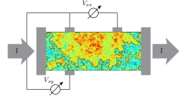
Figure 1: (color online) Two-dimensional sample with percolating random charge inhomogeneities: measurement of longitudinal $V_{xx}$ and Hall $V_{xy}$ voltages with applied current $I$.

General formalism.– Our starting point follows early ideas proposed by several authors Dreizer and Dykhne (1972); Stroud (1975), where effective conductivity approaches were developed based on a local conductivity tensor $\hat{\sigma}(\mathbf{r})$. We consider the general situation of an arbitrary and continuous distribution of conductivity in a macroscopic $d$-dimensional sample of volume $V$, bounded by a surface $S$. The experimentally accessible quantity is the average current density $\langle\mathbf{j}\rangle=\hat{\sigma}_{\mathrm{eff}}\mathbf{E}_{0}$ which is driven by applying a constant electric field $\mathbf{E}_{0}$ at the boundary of the sample. This defines a position-independent effective conductivity tensor $\hat{\sigma}_{\mathrm{eff}}$, which is nothing but the macroscopic conductance tensor, up to a geometrical prefactor. Following Ref. Stroud, 1975, we decompose (arbitrarily at this stage) $\hat{\sigma}(\mathbf{r})=\hat{\sigma}_{0}+\delta\hat{\sigma}(\mathbf{r})$ into uniform and fluctuating parts, respectively. By expressing the electrical field by its scalar potential $\mathbf{E}(\mathbf{r})=-\bm{\nabla}\Phi(\mathbf{r})$, the continuity equation leads to the boundary value problem:

$$\bm{\nabla}\cdot\left[\hat{\sigma}_{0}\bm{\nabla}\Phi(\mathbf{r})\right]=-\bm{\nabla}\cdot\left[\delta\hat{\sigma}(\mathbf{r})\bm{\nabla}\Phi(\mathbf{r})\right]\text{ in V}$$ (2)

$$\Phi(\mathbf{r})\equiv\Phi_{0}(\mathbf{r})=-\mathbf{E}_{0}\cdot\mathbf{r}\text{ on S.}$$ (3)

By introducing the Green’s function $G(\mathbf{r},\mathbf{r^{\prime}})$ defined by

$$\bm{\nabla}\cdot[\hat{\sigma}_{0}\bm{\nabla}G(\mathbf{r},\mathbf{r^{\prime}})]=-\delta(\mathbf{r}-\mathbf{r^{\prime}})\text{ in V}$$ (4)

$$G(\mathbf{r},\mathbf{r^{\prime}})=0\text{ for $\mathbf{r}$ on S,}$$ (5)

the scalar potential is formally given by

$$\Phi(\mathbf{r})=\Phi_{0}(\mathbf{r})+\int_{V}\!\!\!\!d^{d}r^{\prime}\;G(\mathbf{r},\mathbf{r^{\prime}})\bm{\nabla}^{\prime}\cdot[\delta\hat{\sigma}(\mathbf{r^{\prime}})\bm{\nabla}^{\prime}\Phi(\mathbf{r^{\prime}})]$$ (6)

with the short-hand notation $\bm{\nabla}^{\prime}=\bm{\nabla}_{\mathbf{r}^{\prime}}$. Integrating by parts with $\bm{\nabla}^{\prime}G(\mathbf{r},\mathbf{r^{\prime}})=-\bm{\nabla}G(\mathbf{r},\mathbf{r^{\prime}})$ and taking the gradient on both sides of Eq. (6) leads to

$$\mathbf{E}(\mathbf{r}) =\mathbf{E}_{0}+\int_{V}\!\!\!\!d^{d}r^{\prime}\;\bm{\nabla}\cdot\left[\bm{\nabla}G(\mathbf{r},\mathbf{r^{\prime}})\delta\hat{\sigma}(\mathbf{r^{\prime}})\mathbf{E}(\mathbf{r^{\prime}})\right]$$ (7)

$$=\mathbf{E}_{0}+\int_{V}\!\!\!\!d^{d}r^{\prime}\;\hat{\cal{G}}_{0}(\mathbf{r},\mathbf{r^{\prime}})\delta\hat{\sigma}(\mathbf{r^{\prime}})\mathbf{E}(\mathbf{r^{\prime}}),$$ (8)

where $\left[\hat{\cal{G}}_{0}\right]_{ij}=\frac{\partial}{\partial r_{i}}\frac{\partial}{\partial r_{j}}G(\mathbf{r},\mathbf{r^{\prime}})$. Finally, multiplying Eq. (8) by $\delta\hat{\sigma}(\mathbf{r})$ and introducing a new local tensor $\hat{\chi}$ such that $\delta\hat{\sigma}(\mathbf{r})\mathbf{E}(\mathbf{r})=\hat{\chi}(\mathbf{r})\mathbf{E}_{0}$, we obtain:

$$\hat{\chi}(\mathbf{r})\mathbf{E}_{0}=\delta\hat{\sigma}(\mathbf{r})\mathbf{E}_{0}+\delta\hat{\sigma}(\mathbf{r})\int_{V}\!\!\!\!d^{d}r^{\prime}\;\hat{\cal{G}}_{0}(\mathbf{r},\mathbf{r^{\prime}})\hat{\chi}(\mathbf{r^{\prime}})\mathbf{E}_{0}.$$ (9)

As Eq. (9) is valid for all possible choices of $\mathbf{E}_{0}$, the following tensorial equation also holds:

$$\hat{\chi}(\mathbf{r})=\delta\hat{\sigma}(\mathbf{r})+\delta\hat{\sigma}(\mathbf{r})\int_{V}\!\!\!\!d^{d}r^{\prime}\;\hat{\cal{G}}_{0}(\mathbf{r},\mathbf{r^{\prime}})\hat{\chi}(\mathbf{r^{\prime}}).$$ (10)

Spatial averaging of the current $\mathbf{j}(\mathbf{r})=[\hat{\sigma}_{0}+\hat{\chi}(\mathbf{r})]\mathbf{E}_{0}$ over conductivity fluctuations $\delta\hat{\sigma}(\mathbf{r})$ leads therefore to the effective conductivity $\hat{\sigma}_{\mathrm{eff}}=\hat{\sigma}_{0}+\langle\hat{\chi}\rangle$, where the spatial average on $\hat{\chi}$ is performed while enforcing the integral equation (10). Although sample boundaries could be considered in principle, we now focus on an infinite sample, so that the Green’s function [Eq. (4)] becomes translation-invariant

$$G(\mathbf{r},\mathbf{r}^{\prime})=\int\!\!\!\frac{d^{d}p}{(2\pi)^{d}}\frac{e^{i\mathbf{p}\cdot(\mathbf{r}-\mathbf{r}^{\prime})}}{\mathbf{p}\hat{\sigma}_{0}\mathbf{p}+0^{+}},$$ (11)

where $0^{+}$ is a small positive quantity which ensures the correct boundary condition at infinity [Eq. (5)].

Systematic expansion at strong-dissipation.– Previous works either considered a mean-field solution of Eq. (10) in the peculiar case of binary randomness in the local conductivity tensor Stroud (1975), or computed low order contributions for continuous disorder distribution Dreizer and Dykhne (1972); Timm et al. (2005). Our aim is to present a systematic expansion controlled by weak fluctuations of the conductivity and to show that the nonperturbative regime of large conductivity fluctuations can be tackled by sufficient knowledge of the perturbative series. The spatial average on $\hat{\chi}(\mathbf{r})$ can be obtained clearly after iterating Eq. (10) to all orders:

$$\langle\hat{\chi}(\mathbf{r})\rangle= \langle\delta\hat{\sigma}(\mathbf{r})\rangle+\int\!\!d^{d}\mathbf{r}_{1}\langle\delta\hat{\sigma}(\mathbf{r})\hat{\cal{G}}_{0}(\mathbf{r},\mathbf{r}_{1})\delta\hat{\sigma}(\mathbf{r}_{1})\rangle$$ (12)

$$+\int\!\!d^{d}\mathbf{r}_{1}\!\!\int\!\!d^{d}\mathbf{r}_{2}\langle\delta\hat{\sigma}(\mathbf{r})\hat{\cal{G}}_{0}(\mathbf{r},\mathbf{r}_{1})\delta\hat{\sigma}(\mathbf{r}_{1})\hat{\cal{G}}_{0}(\mathbf{r}_{1},\mathbf{r}_{2})\delta\hat{\sigma}(\mathbf{r}_{2})\rangle+...$$

which can be expressed graphically as in Fig. 2.

Figure 2: Graphical representation of the strong-dissipation expansion (12) of the self-consistent transport equation (10).

For incoherent transport, self-averaging occurs and the spatial average over the local conductivity fluctuations may be replaced by an ensemble average.

Let us first illustrate the method for a purely resistive and isotropic medium, so that $\hat{\sigma}_{0}=\sigma_{0}\hat{1}$ and $\delta\hat{\sigma}(\mathbf{r})=\delta\sigma(\mathbf{r})\hat{1}$, with $\left<\delta\sigma(\mathbf{r})\right>=0$. In the limit of strong-dissipation compared to the typical fluctuations of conductivity [$\sigma_{0}\gg\sqrt{\langle\delta\sigma^{2}\rangle}$], we get $\hat{\sigma}_{\mathrm{eff}}=\sigma_{xx}\hat{1}$ with

$$\sigma_{xx} = \sigma_{0}-\frac{1}{\sigma_{0}}\int\!\!d^{d}r\!\!\int\!\!\frac{d^{d}p}{(2\pi)^{d}}\frac{p_{x}^{2}e^{i\mathbf{p}\mathbf{r}}}{\mathbf{p}^{2}+0^{+}}\langle\delta\sigma(\mathbf{r})\delta\sigma(\mathbf{0})\rangle$$

$$= \sigma_{0}-\frac{1}{\sigma_{0}}\int\!\!d^{d}r\;\frac{\delta(\mathbf{r})}{d}\langle\delta\sigma(\mathbf{r})\delta\sigma(\mathbf{0})\rangle=\sigma_{0}-\frac{\langle\delta{\sigma}^{2}\rangle}{d\sigma_{0}}.$$

We thus recover previous results Timm et al. (2005) obtained for weakly disordered media, which predict a reduction of the macroscopic conductance due to randomly distributed resistive barriers. Clearly, nontrivial geometrical aspects are absent at this order, because the dominant background of conductivity $\sigma_{0}$ prevents the percolating network to establish. This general formulation of transport [Eq. (12)] is immediately appealing because arbitrary orders of the strong-dissipation expansion can be generated in a compact fashion, fostering hope that the difficult limit of large conductivity fluctuations can be tackled by standard resummation methods.

Simplification for Gaussian randomness.– Under some microscopic assumptions, the conductivity tensor may follow a random Gaussian distribution, according to $\left<\delta\hat{\sigma}(\mathbf{r})\right>=0$ and $\left<\delta{\sigma}_{ij}(\mathbf{r})\delta{\sigma}_{kl}(\mathbf{r^{\prime}})\right>=C_{ij;kl}(\mathbf{r}-\mathbf{r^{\prime}})$, so that all moments of the local conductivity tensor are determined from Wick’s theorem (in particular, all odd correlations vanish here). This hypothesis leads to a familiar-looking diagrammatic formulation for the strong-dissipation expansion, as shown in Fig. 3.

Figure 3: Diagrammatic expansion in the case of Gaussian fluctuations of the local conductivity. Wiggly lines denote the conductivity correlation functions.

An important technical point is that all particle reducible graphs (diagrams that can be split in two parts by cutting a single line of $\hat{\cal{G}}_{0}$) are identically zero. This is because all such contributions contain the zero momentum limit of the Green’s function $[\hat{\cal{G}}_{0}]_{ij}(\mathbf{p})=-p_{i}p_{j}G(\mathbf{p})$ which vanishes at zero momentum according to Eq. (11) (note the crucial role of the regularization parameter). Interestingly, the conductance correction $\left<\hat{\chi}\right>$ now takes the precise form of a self-energy, in contrast to a fully quantum formulation of electronic transport Akkermans and Montambaux (Cambdrige University Press, 2007) where vertex corrections associated to interference effects need to be accounted for. In what follows, we wish to use the method with the challenging regime of a strongly fluctuating local conductivity, that may lead to geometrical effects related to classical percolation. Clearly, the general perturbation series (12) in powers of $\langle\delta{\hat{\sigma}}^{2}\rangle/\sigma_{0}^{2}$ then breaks down, so that high order terms will be needed.

Percolation regime of the semiclassical Hall effect.– We henceforth consider the semiclassical regime of the quantum Hall effect, which occurs in very high mobility two-dimensional electron gases at large perpendicular magnetic field Zhao et al. (2008); Li et al. (2010). General physical arguments Simon and Halperin (1994) as well as microscopic calculations Geller and Vignale (1994); Champel et al. (2008) show that the electron dynamics can be described in this regime by a local Ohm’s law with a randomly fluctuating Hall conductivity $\sigma_{H}(\mathbf{r})=\sigma_{H}+\delta\sigma(\mathbf{r})$:

$$\hat{\sigma}(\mathbf{r})=\begin{pmatrix}\sigma_{0}&-\sigma_{H}-\delta\sigma(\mathbf{r})\\ \sigma_{H}+\delta\sigma(\mathbf{r})&\;\;\;\;\;\sigma_{0}\end{pmatrix}\;\mathrm{with}\;\langle\delta\sigma(\mathbf{r})\rangle=0.$$ (14)

According to the classical Hall’s law, such purely off-diagonal fluctuations of the conductivity correspond to spatial modulations of the electron density brought by long-range random impurities Simon and Halperin (1994); Ilan et al. (2006). The diagonal part in Eq. (14) accounts phenomenologically for dissipative processes, such as electron-phonon scattering, and is supposed for simplicity to be spatially uniform.

The explicit connection to geometrical percolation can now be made. At vanishing dissipation $\sigma_{0}\to 0$, drift currents follow from Hall’s law and propagate along constant lines of Hall conductivity. Indeed, from Maxwell’s equation $\bm{\nabla}\times\mathbf{E}=0$ and current conservation $\bm{\nabla}\cdot\mathbf{j}=0$, one gets the transport equation $\left[\bm{\nabla}\delta\sigma(\mathbf{r})\right]\cdot\mathbf{j}=0$. The lines of constant $\delta\sigma(\mathbf{r})$ are typically closed, so that all electronic states are localized, except the ones living on the percolation cluster. However, the percolating state does not contribute to macroscopic transport either, as it must necessarily pass through saddle-points of the disordered landscape, where the transport equation becomes undetermined. Thus having finite $\sigma_{0}$ is required to establish a finite conductance in the sample, by connecting the different nearly localized states. This difficulty has led authors Simon and Halperin (1994) to wonder whether purely geometric arguments are sufficient to understand the transport properties at small but finite dissipation, because the current carrying states become broad filaments that may smear the fractal structure of the percolation cluster. This question is now investigated in a controlled fashion.

At high temperature, the Hall conductivity fluctuations given by Eq. (14) follow the Gaussian distribution of disorder Sup . We also consider for simplicity Gaussian spatial correlations $\langle\delta\sigma(\mathbf{r})\delta\sigma(\mathbf{r^{\prime}})\rangle=\langle\delta\sigma^{2}\rangle e^{-|\mathbf{r}-\mathbf{r^{\prime}}|^{2}/\xi^{2}}$, with correlation length $\xi$. Inspection of the diagrammatic series depicted in Fig. 3 shows that the effective conductivity obeys the following expansion:

$$\hat{\sigma}_{\mathrm{eff}}=\begin{pmatrix}0\!&-\sigma_{H}\\ \sigma_{H}\!&0\end{pmatrix}+\sigma_{0}\left[1+\sum_{n=1}^{\infty}a_{n}\frac{\langle\delta\sigma^{2}\rangle^{n}}{\sigma_{0}^{2n}}\right]\begin{pmatrix}1&0\\ 0&1\end{pmatrix}$$ (15)

with dimensionless coefficients $a_{n}$ collecting all diagrams of order $n$ in perturbation theory in $\langle\delta\sigma^{2}\rangle/\sigma_{0}^{2}$. The Hall component is therefore not affected here, while the longitudinal conductance receives nontrivial corrections that encode the interplay of dissipation and percolation. The diagrammatic formulation of transport allowed us to compute this series up to sixth order Sup .

As understood previously, the effective longitudinal conductivity $\sigma_{xx}$ must vanish when $\sigma_{0}\to 0$ for a continuous local conductivity model, and previous works Simon and Halperin (1994); Polyakov and Shklovskii (1995); Fogler and Shklovskii (1995) suggested a power-law dependence $\sigma_{xx}\sim C\langle\delta\sigma^{2}\rangle^{\kappa/2}\sigma_{0}^{1-\kappa}$ at small $\sigma_{0}$, with nonuniversal dimensionless constant $C$ and universal critical exponent $\kappa$ characterizing the transport properties. While $\kappa=10/13$ is often quoted as an exact value Isichenko (1992); Simon and Halperin (1994); Polyakov and Shklovskii (1995); Fogler and Shklovskii (1995), Simon and Halperin  Simon and Halperin (1994) argued that one could not completely rule out the possibility that finite dissipation may spoil the connection to geometrical percolation and change the value of $\kappa$. In order to check that this is not the case, we performed careful Padé resummation Sup of the perturbative series (15) up to six loops, see Table 1.

Order	Method	Exponent $1-\kappa$
2	Padé	$0.28\pm 0.09$
4	Padé	$0.221\pm 0.006$
4	n-fit	$0.233\pm 0.002$
$\infty$	Conjecture	$3/13\simeq 0.2308$

Table 1: Critical exponent $1-\kappa$ obtained from Padé approximants Sup built from the perturbative series (15).

Our most accurate result $\kappa=0.767\pm 0.002$ seems to confirm the conjectured value $\kappa=10/13\simeq 0.7692$ based on the analogy to classical percolation Simon and Halperin (1994); Polyakov and Shklovskii (1995); Fogler and Shklovskii (1995). We stress the good convergence of the Padé approximants for all values of the dissipation strength $\sigma_{0}$, see Fig. 4.

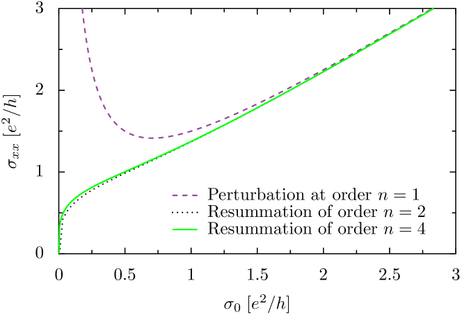
Figure 4: (color online) Scaling function of the longitudinal conductance from the percolating ($\sigma_{0}\to 0$) to the dissipative regime ($\sigma_{0}\to\infty$). A comparison is made between first-order bare perturbation theory (controlled only at large dissipation) to the resummations of the $n=2$ and $n=4$ orders, showing good convergence for all values of $\sigma_{0}$.

Note that partial resummation of perturbation theory in previous works Dreizer and Dykhne (1972) failed to recover the critical behavior associated to percolation in the strong coupling regime and this approximation led to an incorrect saturation of $\sigma_{xx}$ in the limit $\sigma_{0}\to 0$, which would apply only for transport model with discrete conductivity values Dykhne and Ruzin (1994).

Microscopics of $\sigma_{xx}$ at plateau transitions.– We finally study the temperature behavior of transport in the percolation dominated regime. At high magnetic field, the local Hall conductivity is explicitly related to the Fermi distribution of Landau levels $E_{m}=\hbar\omega_{c}(m+1/2)$ with integer $m$, disorder landscape $V(\mathbf{r})$ and chemical potential $\mu$ Geller and Vignale (1994); Champel et al. (2008); Sup :

$$\sigma_{H}(\mathbf{r})=\frac{e^{2}}{h}\sum_{m=0}^{\infty}n_{F}[E_{m}+V(\mathbf{r})-\mu]$$ (16)

neglecting spin effects. We have introduced here the cyclotron energy $\hbar\omega_{c}=\hbar|eB|/m^{\ast}$ in terms of Planck’s constant $\hbar$, electron charge $e$, applied perpendicular magnetic field $B$ and effective mass $m^{\ast}$. At temperatures $T\gg\sqrt{\langle V^{2}\rangle}$, the Fermi distribution $n_{F}(E)$ can be linearized, so that the random conductivity distribution (14) becomes Gaussian. Straightforward analysis Sup and our low-dissipation formula lead to a simple expression for the peak conductance measured at the transition region between two Landau levels ($k_{B}$ is Boltzmann’s constant):

$$\sigma_{xx}^{\mathrm{peak}}=\sigma_{\mathrm{bg}}(T,B)\left[1+\sum_{l=1}^{\infty}\frac{4\pi^{2}lk_{B}T}{\hbar\omega_{c}}\mathrm{csch}\left(\frac{2\pi^{2}lk_{B}T}{\hbar\omega_{c}}\right)\right]^{\kappa}\!\!.$$ (17)

This expression plotted in Fig. 5 shows a sharp crossover at temperature $k_{B}T^{\star}=\hbar\omega_{c}/4$ from a low-$T$ power-law behavior $\sigma_{xx}^{\mathrm{peak}}=\sigma_{\mathrm{bg}}(T,B)[\hbar\omega_{c}/(4k_{B}T)]^{\kappa}$ Polyakov and Shklovskii (1995) to a high-$T$ background conductivity

$$\sigma_{\mathrm{bg}}(T,B)=C[\sigma_{0}(T,B)]^{1-\kappa}\left[\frac{e^{2}}{h}\frac{\sqrt{\langle V^{2}\rangle}}{\hbar\omega_{c}}\right]^{\kappa}\!\!.$$ (18)

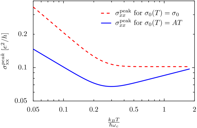
Figure 5: (color online) Temperature dependence of the peak longitudinal conductance from Eq. (17) in log-scale. A crossover occurs at $k_{B}T^{\star}=\hbar\omega_{c}/4$ between a low-$T$ power-law [$\sigma_{xx}\propto T^{-\kappa}$ or $T^{1-2\kappa}$] and a high-$T$ power-law [$\sigma_{xx}\propto\mathrm{cst}$ or $T^{1-\kappa}$], for elastic scattering $\sigma_{0}(T)=\sigma_{0}$ or inelastic phonon scattering $\sigma_{0}(T)=AT$ respectively.

Formulas (17)-(18), which combine microscopic parameters (such as the width of the disorder distribution) with geometrical effects through the exponent $\kappa$, should be useful for detailed analysis of transport measurement in quantum Hall samples.

Clearly, $\sigma_{xx}^{\mathrm{peak}}$ cannot diverge at $T\to 0$ and is in fact expected to level off when reaching conductance values of the order of $e^{2}/2h$ Dykhne and Ruzin (1994); Gammel and Evers (1998). In this very-low-temperature regime, the linearization of the local Hall conductivity (16) breaks down, thereby putting a limit to the present diagrammatic calculation. Furthermore, quantum effects become important at low-$T$ and lead Kramer et al. (2005); Li et al. (2010) to a different exponent $\kappa^{\mathrm{qu.}}\simeq 3/7\simeq 0.42$. The classical percolation exponent Simon and Halperin (1994); Polyakov and Shklovskii (1995); Fogler and Shklovskii (1995) $\kappa=10/13\simeq 0.77$ may be observable in very high mobility samples dominated by smooth disorder Zhao et al. (2008); Li et al. (2010). Finally, at temperatures $T>\hbar\omega_{c}/4$, the leading magnetic field dependence of the longitudinal conductivity in Eq. (17) is provided by the $\omega_{c}^{-\kappa}\propto B^{-\kappa}$ term, as discussed previously Polyakov et al. (2001); Renard et al. (2004).

Conclusion.– We have used a general diagrammatic method to compute fully microscopically the electronic transport in incoherent disordered conductors, leading to accurate determination of critical exponents for the conductivity in the classical percolation regime of the quantum Hall transition. This framework seems also well suited for efficient numerical implementations using the recently developed diagrammatic Monte Carlo methods Gull et al. (2011), leading to envision progresses towards more realistic description of quantum Hall transport taking into account disorder effects.

I Supplementary Material for “Diagrammatic Approach for the High-Temperature Regime of Quantum Hall Transitions”

I.1 Evaluation of the diagrams

We consider here the problem of random Gaussian fluctuations of the local Hall conductivity in two dimensions (see Eq. (14) in the main text), split into an average Hall component $\sigma_{H}$ and a fluctuating term $\delta\sigma(\mathbf{r})$, defined so that $\left<\delta\hat{\sigma}(\mathbf{r})\right>=0$. The dissipationless nature of the Hall component shows up by the fact that $\sigma_{H}$ exactly drops in the correlation function $\left[\hat{\cal{G}}_{0}\right]_{ij}=\frac{\partial}{\partial r_{i}}\frac{\partial}{\partial r_{j}}G(\mathbf{r},\mathbf{r^{\prime}})$:

$$\left[\hat{\cal{G}}_{0}\right]_{ij}(\mathbf{r})=-\frac{1}{\sigma_{0}}\int\!\!\frac{d^{2}p}{(2\pi)^{2}}\frac{p_{i}p_{j}e^{i\mathbf{p}\cdot\mathbf{r}}}{\mathbf{p}^{2}+0^{+}},$$ (1)

with $G(\mathbf{r},\mathbf{r^{\prime}})$ defined by Eq. (11) in the main text.

The first order diagram contributing to the conductivity is straightforwardly calculated in the case of Gaussian fluctuations of the Hall component in two dimensions (see Eq. (14) in the main text):

$$\includegraphics[bb=-3 -3 26 14]{ordnung2.eps}=\int\!\!\frac{d^{2}\mathbf{p}}{(2\pi)^{2}}\tilde{K}(\mathbf{p})\hat{\epsilon}\hat{\cal{G}}_{0}(\mathbf{p})\hat{\epsilon}$$

$$=\frac{\langle\delta\sigma^{2}\rangle}{\pi\sigma_{0}}\!\!\int_{0}^{+\infty}\!\!\!\!\!\!\!\!\!dp\,pe^{-p^{2}}\!\!\!\!\int_{0}^{2\pi}\!\!\!\!\!\!\!d\theta\begin{pmatrix}\sin^{2}(\theta)&-\cos(\theta)\sin(\theta)\\ -\cos(\theta)\sin(\theta)&\cos^{2}(\theta)\end{pmatrix}$$

$$=\frac{\langle\delta\sigma^{2}\rangle}{2\sigma_{0}}\begin{pmatrix}1&0\\ 0&1\end{pmatrix}$$ (2)

with $K(\mathbf{r})\equiv\langle\delta\sigma(\mathbf{r})\delta\sigma(\mathbf{0})\rangle=\langle\delta\sigma^{2}\rangle e^{-|\mathbf{r}|^{2}/\xi^{2}}$, and its Fourier transform $\tilde{K}(\mathbf{p})=\pi\xi^{2}\langle\delta\sigma^{2}\rangle e^{-\xi^{2}\mathbf{p}^{2}/4}$. Here $\hat{\epsilon}$ denotes the fully antisymmetric $2\times 2$ matrix, $\hat{\epsilon}=\big{[}\phantom{\big{[}}_{1}^{0}\phantom{\big{[}}{}_{\phantom{-}0}^{-1}\big{]}$. Note that the conductivity correction [Eq. (2)] is positive and exactly opposite in sign to the one obtained in the case of pure longitudinal fluctuations of the conductivity in Eq. (13) of the main text.

All second and third order diagrams can be obtained analytically with the help of symbolic computation, see the results displayed in Table 1.

Diagram	Multiplicity	Analytical Value	Decimal Value
second order
	1	$-\frac{1}{4}\log(2)$	-0.173287
	1	$\frac{1}{8}(1-\log(4))$	-0.0482868
third order
	1	$\frac{1}{96}\left(3-\pi^{2}+3\log[3](-3+\log[9])+12\mathrm{Polylog}\left[2,\frac{2}{3}\right]\right)$	0.00504001
	2	$\frac{1}{32}\log\left[\frac{27}{16}\right]$	0.0163515
	1	$\frac{1}{16}\left(2\log[2]^{2}-3\log[3]+\log[8]+\mathrm{Polylog}\left[2,\frac{1}{4}\right]\right)$	0.000760209
	2	$\frac{1}{384}(2+100\log[2]-63\log[3])$	0.00547433
	1	$\frac{1}{8}\log\left[\frac{32}{27}\right]$	0.0212374
	1	$\frac{1}{8}\log\left[\frac{27}{16}\right]$	0.065406
	1	$-\frac{1}{48}-\frac{\log[2]}{6}+\frac{9\log[3]}{64}$	0.0181345
	1	$\frac{3}{16}\log\left[\frac{4}{3}\right]$	0.0539404

Table 1: Diagrams to second and third order: multiplicity and analytical values. The resulting coefficients $a_{4}$ and $a_{6}$ are given in Table 3.

The method of computation for the second and third order contributions is to first express each of the several denominators appearing in a given graph using Feynman’s identity:

$$\frac{1}{x_{i}}=\int_{0}^{\infty}\!\!\!\!\!\!dt_{i}\phantom{0}e^{-t_{i}x_{i}}.$$ (3)

One can then perform the Gaussian integration over all momenta, and finally compute the remaining integrals over the auxiliary variables $t_{i}$.

We have not managed to analytically obtain the diagrams of fourth order and beyond (except for the non-crossing ones, see below), and we had therefore recourse to a combination of analytical and numerical steps. First, an automated script was used to generate all possible diagrams, discarding the particle reducible ones, which enables to output explicitely the corresponding functions that require full momentum integration. In order to avoid indefinite integrals, all two-dimensional momenta in an $n^{\mathrm{th}}$ order diagram were combined into the hyperspherical coordinate $\mathbf{K}$ in dimension $2n$, such that $\mathbf{K}^{2}=\sum_{i=1}^{n}{\mathbf{p}_{i}}^{2}$. This allows analytical integration over $|\mathbf{K}|$, leaving the bounded integration domain on the hypersphere in $2n$ dimensions. This numerical step was finally performed using the Vegas Monte Carlo integration routine from the GNU Scientific Library. Because only the complete sum of all diagrams at a given order matters, and since multidimensional integrals are time consuming, we have summed up all the contributions at a given order before performing the integration. The Monte Carlo evaluations were iterated until the relative error was below $0.1\%$, but we can also ascertain the good convergence of the numerics by benchmarking the routine on analytically tractable diagrams that have no crossings of the propagators, see Table 2 for comparison.

Order	Diagram	Analytical value	Monte Carlo evaluation
4		$\frac{-44\log[2]+27\log[3]}{32}\simeq$ -0.02612	-0.02607
5		$\frac{162\log[3]+125\log[5]-544\log[2]}{192}\simeq 0.01084$	0.01087
6		$\frac{-6496\log[2]-486\log[3]+3125\log[5]}{1536}\simeq-0.004632$	-0.004630

Table 2: Benchmarking the numerical Monte Carlo evaluation against analytically tractable non-crossing diagrams at fourth, fifth and sixth order respectively.

The high (up to 6^th) order non-crossing diagrams that we considered are obtained in the following way: we remark that these graphs are only composed of bare propagators and of the first order self-energy $\hat{\Sigma}_{1}$ appearing in Fig. 1.

Figure 1: Self-energy $\hat{\Sigma}_{1}(\mathbf{p})$ entering the calculation of the non-crossing diagrams in Table 2.

The momentum dependence of this self-energy is readily evaluated:

$$\hat{\Sigma}_{1}(\mathbf{p}) = \frac{\langle\delta\sigma^{2}\rangle}{\sigma_{0}}\frac{1}{(p_{x}^{2}+p_{y}^{2})^{2}}\begin{pmatrix}a&b\\ b&c\\ \end{pmatrix},$$ (4)

$$a = \frac{1}{2}(p_{y}^{2}-p_{x}^{2})\left[e^{-p_{x}^{2}-p_{y}^{2}}-1\right]+p_{x}^{2}p_{y}^{2}+p_{y}^{4},$$

$$b = -p_{x}p_{y}[e^{-p_{x}^{2}-p_{y}^{2}}-1+p_{x}^{2}+p_{y}^{2}],$$

$$c = \frac{1}{2}(p_{x}^{2}-p_{y}^{2})\left[e^{-p_{x}^{2}-p_{y}^{2}}-1\right]+p_{x}^{2}p_{y}^{2}+p_{x}^{4}.$$

We note that $\hat{\Sigma}_{1}(\mathbf{p}=\mathbf{0})$ recovers the first order contribution to the conductivity in Eq. (2). At finite momentum, the self-energy contains off-diagonal elements, although the final correction to the conductivity is purely diagonal. The analytical computation of the non-crossing diagrams then proceeds as previously described, using Feynman’s trick and Gaussian integration. For instance the following fourth order contribution

$$\includegraphics[width=56.9055pt]{ordnung8plat_8234567.eps}=\int\!\!\frac{d^{2}p}{(2\pi)^{2}}\tilde{K}(\mathbf{p})\hat{\epsilon}\hat{\cal{G}}_{0}(\mathbf{p})[\hat{\Sigma}_{1}(\mathbf{p})\hat{\cal{G}}_{0}(\mathbf{p})]^{3}\hat{\epsilon}$$

only involves a single momentum integration, which can then be performed analytically. Its value is given in Table 2.

I.2 Extrapolation to the weak dissipation regime

We present here the methodology to obtain the extrapolated behaviour of the effective diagonal conductivity in the limit $\sigma_{0}\to 0$, starting from the large-$\sigma_{0}$ expansion:

$$\sigma_{xx}(\sigma_{0})=\sigma_{0}\left[1+\sum_{n=1}^{\infty}a_{n}\frac{\langle\delta\sigma^{2}\rangle^{n}}{\sigma_{0}^{2n}}\right]$$ (5)

with the first six coefficients $a_{n}$ given in Table 3.

Order	Method	Coefficient $a_{n}$
1	Analytical	$\frac{1}{2}$
2	Analytical	$\frac{1}{8}-\frac{1}{2}\log(2)$
3	Analytical	$0.2034560502$
4	Numerical	$-0.265\pm 0.001$
5	Numerical	$0.405\pm 0.001$
6	Numerical	$-0.694\pm 0.001$

Table 3: Coefficients $a_{n}$ of the perturbative series (5) up to sixth loop order.

One standard method of extrapolation is the so-called DLog Padé approximants Singh and Chakravarty (1987), which starts with the dimensionless logarithmic derivative of the function to extrapolate:

$$f(x)\equiv\frac{\sigma_{0}}{\sigma_{xx}(\sigma_{0})}\frac{\mathrm{d}\sigma_{xx}(\sigma_{0})}{\mathrm{d}\sigma_{0}}_{\big{|}\sigma_{0}/\sqrt{\langle\delta\sigma^{2}\rangle}\to x}.$$ (6)

One then reexpands at small $x$ the function $f(x)$ to order $N$:

$$f_{N}(x)=1+\sum_{n=1}^{N}b_{n}x^{2n}$$ (7)

with the coefficients $b_{n}$ given in Table 4.

Order	1	2	3	4	5	6
Coefficient $b_{n}$	-1	$\log(4)$	-2.135	3.698	-6.919	13.823

Table 4: Coefficients $b_{n}$ used in the DLog Padé extrapolation, corresponding to the small-$x$ series expansion (7) of the function $f(x)$ defined in Eq. (6).

The DLog Padé method uses then an approximant for $f(x)$ of the following form:

$$f_{N}(x)=\frac{1+\sum_{n=1}^{N}c_{n}x^{2n}}{1+\sum_{p=1}^{N}d_{n}x^{2n}}.$$ (8)

The coefficients $c_{n}$ and $d_{n}$ are computed from the knowledge of the perturbative terms $b_{n}$ given in Table 4. ¿From the expected power-law behavior of the conductivity at small dissipation, $\sigma_{xx}\propto\langle\delta\sigma^{2}\rangle^{\kappa/2}\sigma_{0}^{1-\kappa}$, one gets $f(x)\to(1-\kappa)$ for $x\to\infty$. The critical exponent $\kappa$ is thus obtained by extrapolating the Padé approximant (8) to infinity, which simply reads $1-\kappa=c_{N}/b_{N}$ at the order $N$.

The corrections to the effective conductivity at second order require an order $N=2$ DLog Padé approximant, which lead after integration of Eq. (6) to the formula:

$$\sigma_{xx}\simeq\sigma_{0}\left[1+\frac{1}{\kappa}\frac{\langle\delta\sigma^{2}\rangle}{\sigma_{0}^{2}}\right]^{\kappa/2}$$ (9)

with $\kappa=0.72\pm 0.09$. The error bar on $\kappa$ is obtained here by expanding Eq. (9) to third order with $\kappa$ arbitrary, and comparing the deviation from the resulting coefficient with the exact $a_{3}$ value. Eq. (9) captures the full crossover between the perturbative regime $\langle\delta\sigma^{2}\rangle\ll\sigma_{0}^{2}$ (where strong dissipation controls transport) to the non-perturbative limit of vanishing dissipation $\sigma_{0}\to 0$ (where percolation effects dominate), see Fig. 4 in the main text.

In order to obtain a better estimate for the exponent, one must push the calculation of the effective conductivity to fourth order. Following the same strategy, the order $N=4$ DLog Padé approximant provides the estimate $\kappa=0.779\pm 0.006$, and the resulting formula for the effective conductivity takes the form:

$$\sigma_{xx}(\sigma_{0})=\sigma_{0}\left(1+A\frac{\langle\delta\sigma^{2}\rangle}{\sigma_{0}^{2}}\right)^{B}\left(1+C\frac{\langle\delta\sigma^{2}\rangle}{\sigma_{0}^{2}}\right)^{D}$$ (10)

with dimensionless numbers $A,B,C,D$, leading to $\kappa=2B+2D$. Again, the error bar on $\kappa$ is obtained from comparison to the next known coefficient, namely $a_{5}$, expanding Eq. (10) to fifth order while keeping an arbitrary $\kappa$ fixed (a small additional error due to the Monte Carlo evaluation of the coefficients was also taken into account).

While our calculation of the sixth order corrections to the conductivity would allow us in principle to further refine the estimation of the exponent, we encounter in that case a spurious pole Watts (1975), that invalidates the method. One explanation why the Padé method becomes unstable at high orders can be understood already from the fourth order extrapolation (10), which leads to trivial sub-leading corrections to scaling at small dissipation:

$$\sigma_{xx}(\sigma_{0})\propto\langle\delta\sigma^{2}\rangle^{\kappa/2}\sigma_{0}^{1-\kappa}\,\left[1+E\frac{\sigma_{0}^{2}}{\langle\delta\sigma^{2}\rangle}+\dots\right].$$ (11)

This shows that the DLog Padé method enforces a given value $\kappa^{\prime}\simeq 3-\kappa$ for the sub-leading exponent $\kappa^{\prime}$, which is unlikely to correspond with good precision to the right value. This lack of flexibility is the likely source of the instability of the Padé approximant, and authors Ferer and Velgakis (1983) have used a generalized n-Fit method that circumvents this problem. For the case of the fourth order conductivity, the fitting formula has rather the following additive form:

$$\sigma_{xx}(\sigma_{0})=F\sigma_{0}\left(1+G\frac{\langle\delta\sigma^{2}\rangle}{\sigma_{0}^{2}}\right)^{H}\!\!\!\!+(1-F)c_{0}\left(1+I\frac{\langle\delta\sigma^{2}\rangle}{\sigma_{0}^{2}}\right)^{J}\!\!\!\!.$$ (12)

The critical exponent is then given by $\kappa=\min[2H,2J]$, while the independent subleading exponent reads $\kappa^{\prime}=\max[2H,2J]$. All unknown numerical coefficients are obtained by expanding Eq. (12) at small $x$ and fitting to the coefficients of Table 4. Estimating the error by comparison to the known $a_{5}$ coefficient, we find $\kappa=0.767\pm 0.002$, in excellent agreement with the conjectured value $\kappa=10/13\simeq 0.7692$. Moreover, the Padé approximants show good convergence for all values of the dissipation strength $\sigma_{0}$, see Fig. 4 in the main text.

I.3 High temperature microscopics of ${\bm{\sigma}_{xx}}$ at the plateau transition

The local Hall conductivity can be computed microscopically in the high magnetic field regime Geller and Vignale (1994); Champel et al. (2008), and simply follows from Hall’s law with Landau level quantization:

$$\sigma_{H}(\mathbf{r})=\frac{e^{2}}{h}\sum_{m=0}^{\infty}n_{F}[E_{m}+V(\mathbf{r})-\mu]$$ (13)

with standard Landau levels $E_{m}=\hbar\omega_{c}(m+1/2)$, cyclotron frequency $\omega_{c}=|eB|/m^{\ast}$, random disorder potential $V(\mathbf{r})$, chemical potential $\mu$ and Fermi function $n_{F}(E)=1/\{\exp[E/(k_{B}T)]+1\}$. In particular, microscopic calculations Champel et al. (2008) show that deviations to the form (13) are small by the dimensionless parameter $[l_{B}^{2}\sqrt{\langle V^{2}\rangle}]/[\xi^{2}\hbar\omega_{c}]\ll 1$, with $\sqrt{\langle V^{2}\rangle}$ the width of the disorder distribution, $l_{B}=\sqrt{h/|eB|}$ the magnetic length, and $\xi$ the large correlation length of the disorder fluctuations. Note the smallness of $l_{B}\simeq 8$nm at $B=10$T, so that $l_{B}\ll\xi$ for smooth disorder.

At temperatures such that $T\gg\sqrt{\langle V^{2}\rangle}$, the Fermi distribution in Eq. (13) can be linearized, so that Gaussian fluctuations of disorder provide Gaussian fluctuations for the Hall conductivity $\sigma_{H}(\mathbf{r})=\sigma_{H}+\delta\sigma(\mathbf{r})$ with

$$\sigma_{H} = \frac{e^{2}}{h}\sum_{m=0}^{\infty}n_{F}(E_{m}-\mu),$$ (14)

$$\delta\sigma(\mathbf{r}) = \frac{e^{2}}{h}\sum_{m=0}^{\infty}n_{F}^{\prime}(E_{m}-\mu)V(\mathbf{r}).$$ (15)

The power-law behavior of the longitudinal conductivity at small dissipation, $\sigma_{xx}=C\sigma_{0}^{1-\kappa}\langle\delta\sigma^{2}\rangle^{\kappa/2}$, leads to:

$$\sigma_{xx}=C\sigma_{0}^{1-\kappa}\left|\frac{e^{2}}{h}\sqrt{\langle V^{2}\rangle}\sum_{m=0}^{\infty}n_{F}^{\prime}(E_{m}-\mu)\right|^{\kappa}\!.$$ (16)

We re-express the sum over Landau levels in Eq. (16) by using Poisson summation formula:

$$\sum_{m=0}^{+\infty}f(m)=\sum_{l=-\infty}^{+\infty}\int_{0}^{+\infty}\!\!\!\!\!dt\,e^{i2\pi lt}f(t).$$ (17)

In the limit $T<\mu$, one finds after standard manipulations Champel and Mineev (2001):

$$\left|\sum_{m=0}^{\infty}n_{F}^{\prime}(E_{m}-\mu)\right| = \frac{1}{\hbar\omega_{c}}\Bigg{[}1+\sum_{l=1}^{+\infty}(-1)^{l}\cos\left(\frac{2\pi l\mu}{\hbar\omega_{c}}\right)$$ (18)

$$\times\frac{\frac{4\pi^{2}lk_{B}T}{\hbar\omega_{c}}}{\mathrm{sinh}\left(\frac{2\pi^{2}lk_{B}T}{\hbar\omega_{c}}\right)}\Bigg{]}.$$

Finally, by considering the plateau transition region between the filling factors $\nu$ and $\nu+1$, the chemical potential is pinned to $\mu=\hbar\omega_{c}(\nu+1/2)$, leading to expressions (17)-(18) in the main text.

References

- Singh and Chakravarty (1987) R. R. P. Singh and S. Chakravarty, Phys. Rev. B 36, 559 (1987).
- Watts (1975) M. G. Watts, J. Phys. A: Math. Gen. 8, 61 (1975).
- Ferer and Velgakis (1983) M. Ferer and M. J. Velgakis, Phys. Rev. B 27, 2839 (1983).
- Geller and Vignale (1994) M. R. Geller and G. Vignale, Phys. Rev. B 50, 11714 (1994).
- Champel et al. (2008) T. Champel, S. Florens, and L. Canet, Phys. Rev. B 78, 125302 (2008).
- Champel and Mineev (2001) T. Champel and V. P. Mineev, Philos. Mag. B 81, 55 (2001).