Boost-invariant Leptonic Observables and Reconstruction of Parent Particle Mass

Abstract

We propose a class of observables constructed from lepton energy distribution, which are independent of the velocity of the parent particle if it is scalar or unpolarized. These observables may be used to measure properties of various particles in the LHC experiments. We demonstrate their usage in a determination of the Higgs boson mass.

The data and analyses from the experiments at the CERN Large Hadron Collider (LHC) are attracting increasing attention. The main goals of these experiments are discoveries of the Higgs boson and of signals of physics beyond the Standard Model. Once the Higgs boson or other new particles are found, the next step is to uncover properties of these particles. There are well-known challenges in performing accurate measurements for such purposes: (i) In reconstructing the kinematics of events, it is difficult to reconstruct jet energy scales accurately. This is in contrast to electron and muon energy-momenta, which can be measured fairly accurately. (ii) Often interesting events include undetected particles which carry off missing momenta. In this case, reconstruction of missing momenta is non-trivial. (iii) The parton distribution function (PDF) of proton is needed in predicting cross sections and kinematical distributions. Our current knowledge of PDF is limited, which induces relatively large uncertainties in these predictions. As a consequence of these difficulties, for instance, it is difficult to measure the energy-momentum of a produced new particle or predict accurately their statistical distributions.

To circumvent these difficulties, many sophisticated methods for kinematical reconstruction of events have been devised. See, for instance, Barr:2003rg ; Barr:2010zj and references therein. In these methods, one takes advantage of various kinematical constraints, which follow from specific event topologies, to complement uncertainties induced by the above difficulties. Still, in most cases challenges remain to reduce systematic uncertainties originating from ambiguities in jet energy scales, PDF and other non-perturbative or higher-order QCD effects. Generally it is quite non-trivial to keep these uncertainties under control, both theoretically and experimentally.

In this paper we propose a class of observables which can be used to measure properties of particles produced in the LHC experiments, by largely avoiding the above uncertainties. We consider a particle $X$ which is scalar or unpolarized and whose decay daughters include one or more charged leptons $\ell$$=e^{\pm}$ or $\mu^{\pm}$. The observables are constructed from the energy distribution of $\ell$ and are independent of the velocity of $X$. Although experimental cuts and backgrounds induce corrections to this property, we will show that systematic uncertainties are suppressed and can be kept under control. Furthermore, we can utilize the degree of freedom of the observables to reduce or control effects induced by cuts and backgrounds.

In the first part of the paper, we explain the construction of these observables, in the two-body decay and multi-body decay cases separately. In the latter part, we demonstrate its usefulness in a determination of the Higgs boson mass using the vector-boson fusion process.

2-body decay: $X\to\ell+Y$

Suppose a parent particle $X$ decays into two particles, one of which is a lepton $\ell$ whose energy is $E_{0}$ (monochromatic) in the rest frame of $X$. In the case that $X$ is scalar or unpolarized, the normalized lepton energy distribution in a boosted frame, in which $X$ has a velocity $\beta$, is given by

$${\cal D}_{\beta}(E_{\ell};E_{0})=\frac{1}{(e^{y}-e^{-y})E_{0}}\,\theta(e^{-y}E_{0}<E_{\ell}<e^{y}E_{0}),$$ (1)

in the limit where the mass of the lepton is neglected. Here, $y$ is the rapidity of $X$ in the boost direction, related to $\beta$ as $e^{2y}=(1+\beta)/(1-\beta)$. The step function is defined such that $\theta(cond.)=1$ if $cond.$ is satisfied, and $\theta(cond.)=0$ otherwise.

We construct an observable $g(E_{\ell}/E_{0})$ from the lepton energy $E_{\ell}$ in the boosted frame such that the expectation value $\langle g\rangle$ is independent of $\beta$. For later convenience, we write $g(E_{\ell}/E_{0})=[dG(x)/dx]_{x=E_{\ell}/E_{0}}$. Hence,

$$\left\langle g\right\rangle\!=\!\int\!\!dE_{\ell}\,{\cal D}_{\beta}(E_{\ell};E_{0})\,g(E_{\ell}/E_{0})=\frac{G(e^{y})-G(e^{-y})}{e^{y}-e^{-y}}\,.$$ (2)

This shows that $\langle g\rangle$ is the even part $F(y)+F(-y)$ of $F(y)\equiv G(e^{y})/(e^{y}-e^{-y})$. It is $\beta$($y$)-independent when $F$ is an odd function of $y$ plus a constant independent of $y$. Namely, $G(e^{y})=(\mbox{even fn.\ of $y$})+const.\times(e^{y}-e^{-y})$.

Let us demonstrate usage of $\langle g\rangle$. In the case $G=e^{y}-e^{-y}$, we obtain $\langle 1/E_{\ell}^{2}\rangle=1/E_{0}^{2}$. Thus, (mathematically) we can reconstruct $E_{0}$ from the lepton energy distribution irrespective of $\beta$ of the parent particle. In the case $G(e^{y})=(\mbox{even fn.\ of $y$})$, $\left\langle g(E_{\ell}/E_{0})\right\rangle=0$. Conversely, we can adjust $E_{0}$, which enters $g(E_{\ell}/E_{0})$ as an external parameter, such that $\langle g\rangle$ vanishes and determine the true value of $E_{0}$. We give two examples of $G$ for the latter case: (a) $G^{(a)}_{n}={1}/[2\,n\,{\cosh(ny)}]$, corresponding to $g=E_{0}^{n+1}E_{\ell}^{n-1}(E_{0}^{2n}-E_{\ell}^{2n})/(E_{0}^{2n}+E_{\ell}^{2n})^{2}$. As $n$ increases, contributions of the $E_{\ell}$ distribution from large $|y|$ region ($E_{\ell}\ll E_{0}$ or $E_{\ell}\gg E_{0}$) become more suppressed. (b) $G^{(b)}_{r}=\theta(r<e^{-|y|}<1)(e^{-|y|}-r)$, corresponding to $g=\theta(r<E_{\ell}/E_{0}<1)-(E_{0}/E_{\ell})^{2}\theta(1<E_{\ell}/E_{0}<r^{-1})$. This observable is independent of the $E_{\ell}$ distribution in the regions $E_{\ell}<rE_{0}$ and $E_{\ell}>r^{-1}E_{0}$.

Many-body decay: $X\to\ell+{\rm anything}$

We assume that we know the theoretical prediction for the lepton energy distribution in the rest frame of the parent particle $X$, ${d\Gamma_{X\to\ell+{\rm anything}}}/{dE_{0}}\,,$ where $E_{0}$ is the lepton energy in this frame. We define an observable in the boosted frame as

$${\cal O}_{G}\equiv{\cal N}\int\frac{dE_{0}}{E_{0}^{2}}\,\frac{d\Gamma_{X\to\ell+{\rm anything}}}{dE_{0}}\,\left[\frac{d}{dx}\,G(x)\right]_{x=E_{\ell}/E_{0}}\,.$$ (3)

It depends on the lepton energy $E_{\ell}$ in the boosted frame and on the parameters of $d\Gamma/dE_{0}$ such as the parent particle mass $m_{X}$. $\cal N$ is an arbitrary normalization constant independent of $E_{l}$. We can prove (see below) that, if $X$ is scalar or unpolarized, and if we take the same $G$ as in the 2-body decay case, $\langle{\cal O}_{G}\rangle$ is independent of $\beta$ of $X$. In particular, in the case that $G(e^{y})$ is an even function of $y$, $\langle{\cal O}_{G}\rangle=0$. The parent particle mass enters as an external parameter in the definition of ${\cal O}_{G}$. Hence, we can use this property to determine $m_{X}$, provided that other parameters are known. $g$ in the 2-body decay case can be regarded as a special case of ${\cal O}_{G}$.

Proof:  The lepton energy distribution in the boosted frame is given by

$$f_{\beta}(E_{\ell})=\int dE^{\prime}_{0}\,\frac{d\Gamma_{X\to\ell+{\rm anything}}}{dE^{\prime}_{0}}\,{{\cal D}_{\beta}(E_{\ell};E^{\prime}_{0})}\,.$$ (4)

Hence,

$$\langle{\cal O}_{G}\rangle=\int dE_{\ell}\,f_{\beta}(E_{\ell})\,{\cal O}_{G}$$

$$={\cal N}\int dE_{0}dE^{\prime}_{0}\,\frac{d\Gamma}{dE_{0}}\frac{d\Gamma}{dE^{\prime}_{0}}\,\frac{G(e^{y}E^{\prime}_{0}/E_{0})-G(e^{-y}E^{\prime}_{0}/E_{0})}{E_{0}\,E^{\prime}_{0}\,(e^{y}-e^{-y})}\,,$$

where we integrated over $E_{\ell}$. In the case $G(x^{-1})=G(x)$, $G(e^{y}E^{\prime}_{0}/E_{0})-G(e^{-y}E^{\prime}_{0}/E_{0})=G(e^{y}E^{\prime}_{0}/E_{0})-G(e^{y}E_{0}/E^{\prime}_{0})$ is anti-symmetric under the exchange of $E_{0}$ and $E^{\prime}_{0}$, while all other parts are symmetric. It follows that $\langle{\cal O}_{G}\rangle=0$. In the case $G(x)=x-x^{-1}$, $G(e^{y}E^{\prime}_{0}/E_{0})-G(e^{-y}E^{\prime}_{0}/E_{0})=(E^{\prime}_{0}/E_{0}+E_{0}/E^{\prime}_{0})(e^{y}-e^{-y})$, so that $y$-dependence cancels out. (Q.E.D.)

Since we must know the theoretical prediction for $d\Gamma/dE_{0}$ to construct ${\cal O}_{G}$, we consider use of ${\cal O}_{G}$ mainly for the purpose of precision measurements, after the nature of the parent particle (such as its decay modes) is roughly determined by other methods. In principle, different functions $G$ in constructing ${\cal O}_{G}$ may be used to determine simultaneously more than one parameters in a decay process. In this first study, however, we consider the case where only one parameter is unknown.

Under a realistic experimental condition, in which $\beta$ of $X$ has a distribution $D_{X}(\beta)$, the lepton energy distribution in the laboratory frame is given by $D(E_{\ell})=\int d\beta\,D_{X}(\beta)f_{\beta}(E_{\ell})$. In this case, the expectation value $\langle{\cal O}_{G}\rangle_{D}\equiv\int dE_{\ell}\,D(E_{\ell})\,{\cal O}_{G}$ is independent of $D_{X}$. Hereafter, we choose $G$ to be an even function of $y$ and use $\langle{\cal O}_{G}\rangle_{D}=0$ to determine $m_{X}$. Generally various experimental cuts, which affect $D(E_{\ell})$, are imposed due to detector acceptance effects and for event selection purposes. Furthermore, there are contributions from background processes which also modify $D(E_{\ell})$. After incorporating these effects, there is no guarantee for $\langle{\cal O}_{G}\rangle$ to vanish. Suppose that $D(E_{\ell})$ is modified to $D(E_{\ell})+\delta D(E_{\ell})$ by these effects, where the distributions are normalized as $\int dE_{\ell}\,D=\int dE_{\ell}\,(D+\delta D)=1$. In the case $|\delta D/D|\ll 1$, if $\langle{\cal O}_{G}\rangle_{D+\delta D}=0$ is used to extract $m_{X}$, the obtained value is systematically shifted from the true value by an amount

$$\delta m_{X}=-\langle{\cal O}_{G}\rangle_{\delta D}\biggl{/}\left\langle\frac{\partial{\cal O}_{G}}{\partial m_{X}}\right\rangle_{D},$$ (6)

where we neglected ${O}(\delta D^{2})$ corrections. We can use this formula to study systematic corrections in the determination of $m_{X}$. $\delta D$ should be estimated by Monte Carlo (MC) simulations which take into account realistic experimental conditions. Errors in the estimate of $\delta D$ contribute as systematic uncertainties in the determination of $m_{X}$.

The production of Higgs bosons via vector-boson fusions is expected to be observed with a good signal-to-noise ratio, if the Higgs boson mass $m_{H}$ is within the range $135~{}{\rm GeV}\hbox{ \raise 3.0pt\hbox to0.0pt{$<$}\raise-3.0pt\hbox{$\sim$} }m_{H}\hbox{ \raise 3.0pt\hbox to0.0pt{$<$}\raise-3.0pt\hbox{$\sim$} }190~{}{\rm GeV}$, hence it is considered as a promising channel for the Higgs boson discovery. We perform a MC simulation to study feasibility of $m_{H}$ determination using the observable ${\cal O}_{G}$ and the decay modes $H\to WW^{(*)}\to\ell\ell\nu\nu$ ($\ell\ell=e\mu,\mu\mu,ee$). We generate the events for the signal and background processes using MadEvent Maltoni:2002qb , which are passed to PYTHIA Sjostrand:2006za and then to the fast detector simulator PGS PGS . We set $\sqrt{s}=14$ TeV.

The strategy of our analysis follows, to a large extent, that of Asai:2004ws , which studied the prospect of Higgs boson search using the vector-boson fusion process in the ATLAS experiment. We first repeated the analysis of Asai:2004ws in the case of $H\to e\mu\nu\nu$ mode using our analysis tools and imposing the same cuts. We reproduced the numbers in Tab. 4 of Asai:2004ws reasonably well, considering differences in both analyses, such as different detector simulators, different PDF’s, and different jet clustering algorithms (we use the cone algorithm with $R=0.5$; we do not correct the jet energy scales given by the output of PGS): regarding the signal events, we reproduced the efficiencies of the cuts involving only leptons within a few % accuracy and those involving jets within a few tens % accuracy; in total, the efficiency of all the cuts was reproduced with 6% accuracy. On the other hand, the cross section of the signal is smaller by 30% in our analysis as compared to that of Asai:2004ws . The difference originates from the different scales and different PDF’s used in the event generators. We do not correct the difference in normalization of the cross sections; it may result in overestimates of the statistical errors given below.

For simplicity, in our analysis we omit the Higgs boson production via $gg$ fusion and the Higgs decay modes including $\tau$’s. In principle, part of these modes including $e$ or $\mu$ in the final states can be used as signal events, since $d\Gamma_{H\to\ell+{\rm anything}}/dE_{0}$ is calculable.

In our analysis of $m_{H}$ reconstruction, ideally two criteria need to be satisfied to ensure use of the observable ${\cal O}_{G}$: (1) The lepton energy distribution in the Higgs rest frame agrees with the theoretical prediction $d\Gamma_{H\to\ell\ell\nu\nu}/dE_{0}$. (2) The lepton angular distribution in the Higgs rest frame is isotropic. The effects of cuts should not violate these criteria significantly.

Jets in the signal process are associated with the Higgs production process and are independent of the Higgs decay process. Therefore, cuts involving only jets would not affect the above criteria but only affect the $\beta$ distribution of the Higgs boson. By contrast, cuts involving leptons can affect the above criteria significantly.

Taking this into account, we use the same cuts as in Asai:2004ws except the following two cuts:
(A) Lepton acceptance
       No muon isolation requirement;
       $P_{T}(e)>15$ GeV, $P_{T}(\mu)>10$ GeV, $|\eta_{\ell}|<2.5$;
       Only one pair of identified leptons in each event.
(B) Lepton cuts
       $M_{\ell\ell}<45$ GeV,   $P_{T}(e),P_{T}(\mu)<120$ GeV.
Concerning (A), since lepton isolation requirement as well as cuts on lepton $P_{T}$ and $\eta$ bias the lepton angular distribution in the Higgs rest frame, we loosen the cuts and requirement as much as possible. Concerning (B), it is important to select events with leptons in the same directions, in order to reduce background events. We note that, if we impose the same cut on $M_{\ell\ell}$ in the theoretical prediction for $d\Gamma_{H\to\ell\ell\nu\nu}/dE_{0}$, this cut does not contribute to systematic errors. Hence, we tighten the Lorentz invariant cut and omit other frame-dependent angular cuts. By modification of the cuts (A) and (B), the efficiency of the signal events reduces by a few tens %, while variations of the efficiencies of the background events are small.

	Signal ($m_{H}$)			Background
	150 GeV	180 GeV	200 GeV	$t\bar{t}+Wt$	$WW$+jets
$e\mu$ mode [fb]	2.00	2.21	1.07	0.53	0.13
$\mu\mu$ mode [fb]	1.33	1.47	0.68	0.31	0.05
$ee$ mode [fb]	0.76	0.89	0.42	0.24	0.04

Table 1: Cross section$\times$efficiency, after all the cuts. $e,\mu$ from $\tau$ are not included.

Tab. 1 lists estimates of (cross section)$\times$(efficiency) of the signal and background events, after all the cuts are imposed. For the backgrounds, we simulate only $t\bar{t}+Wt$ and $WW$+jet (electroweak) events, which are shown to be the major backgrounds in Asai:2004ws . We estimate contributions of other backgrounds to be negligible, compared to the uncertainties discussed below. Consistently with the signal, we omit background events with $\ell=e,\mu$ from $\tau$.

We test the two criteria with the signal events which passed all the cuts. The histogram in Fig. 1 shows the lepton ($\ell=\mu$) energy distribution in the Higgs rest frame for the $H\to\mu\mu\nu\nu$ mode and MC input $m_{H}^{\rm MC}=150$ GeV, where we looked up the parton-level neutrino momenta in each event to reconstruct the Higgs momentum. We generated a large-statistics event sample (about 12,000 events after applying all the cuts) in order to focus on the systematic effects caused by the cuts. The theoretical prediction for $d\Gamma_{H\to\ell\ell\nu\nu}/dE_{0}$ with the cut $M_{\ell\ell}<45$ GeV (no other cuts are applied) is also plotted with a red line. A good agreement is observed.

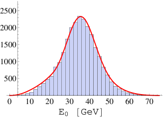
Figure 1: Lepton energy distribution in the Higgs rest frame.

Figs. 2 show the lepton $\cos\theta$ distributions in the Higgs rest frame of these events, where $\theta$ is the angle measured from the Higgs boost direction. The total event sample is divided into four groups of equal size, in the increasing order of $\beta$ (or $y$) of the Higgs boson. The average $y$ value for each group is displayed. The events with low $y$ have a distribution closer to isotropic one, whereas the events with large boost factors have strong distortion of the $\cos\theta$ distribution. Since Higgs bosons with large $y$ are boosted mostly in the beam directions, the lepton $P_{T}$ and $\eta$ cuts and electron isolation requirement bias the $\cos\theta$ distribution. In particular, depletion of events in the $\cos\theta\simeq 1$ region of large $y$ samples is caused by the lepton $\eta$ cuts. On the other hand, Higgs bosons with small $y$ are boosted in random directions, so that the lepton acceptance effects do not bias the lepton $\cos\theta$ distribution strongly. Thus, the second criterion is satisfied only by events with small boost factors.

We may choose $G$ appropriately to suppress contributions of events with large $y$. By examining various $G$, we find that $G=G^{(a)}_{n}$ for $n\approx 4$ is an optimal choice. As $n$ increases, $\langle{\cal O}_{G}\rangle$ becomes less sensitive to events with large $y$ but more sensitive to statistical fluctuations.

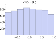
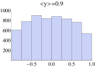
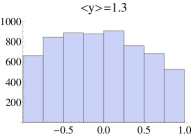
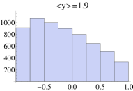
Figure 2: Lepton $\cos\theta$ distribution in the Higgs rest frame.

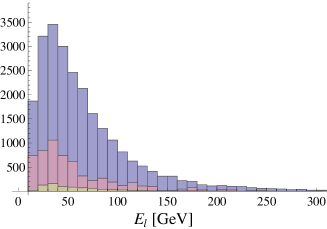
Figure 3: Muon energy distribution after applying all the cuts for $H\to\mu\mu\nu\nu$ mode. Histograms represent muons from the signal (corresponding to $m_{H}^{\rm MC}=150$ GeV), $t\bar{t}+Wt$ and $WW$+jet events (overlayed, from back to front).

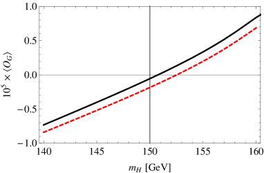
Figure 4: $10^{5}\times\langle{\cal O}_{G}\rangle$ as a function of $m_{H}$ in the theoretical prediction for $d\Gamma_{H\to\ell\ell\nu\nu}/dE_{0}|_{M_{\ell\ell}<45{\rm GeV}}$. Muon energy distribution given in Fig. 3 is used: solid (dashed) line represents the expectation value taken with respect to the signal–plus–background (signal) MC events.

In $m_{H}$ determination, typically there are two solutions which satisfy $\langle{\cal O}_{G}\rangle=0$, one above and one below the $WW$ threshold $2M_{W}$. We believe that, unless $m_{H}$ is very close to $2M_{W}$ , the correct solution can be identified relatively easily, using profiles of the lepton energy distribution, dilepton invariant mass distribution, etc. Hence, we consider deviations only around the correct solution.

Fig. 3 shows the muon energy distributions separately for the signal events and the $t\bar{t}+Wt$ and $WW$+jet background events, which passed through all the cuts for the $H\to\mu\mu\nu\nu$ mode. The signal events are generated with $m_{H}^{\rm MC}=150$ GeV and the number of events after the cuts is about 12,000. The normalizations of the background events have been rescaled according to the respective cross sections to match the number of the signal events. Using this distribution the expectation value $\langle{\cal O}_{G}\rangle$ is computed; see Fig. 4. The observable ${\cal O}_{G}$ in eq. (3) is defined with $G=G^{(a)}_{n=4}$ and the theoretical prediction for $d\Gamma_{H\to\ell\ell\nu\nu}/dE_{0}$ is computed imposing a cut ${M_{\ell\ell}<45~{}{\rm GeV}}$ on the dilepton invariant mass. The value of $\langle{\cal O}_{G}\rangle$ changes as a function of $m_{H}$, which enters as an external parameter in the theoretical prediction for $d\Gamma_{H\to\ell\ell\nu\nu}/dE_{0}|_{M_{\ell\ell}<45{\rm GeV}}$. Without any cuts and without background contributions, $\langle{\cal O}_{G}\rangle$ would cross zero at $m_{H}=150$ GeV in the large statistics limit. As seen in Fig. 4, due to the effects of the cuts, the expectation value $\langle{\cal O}_{G}\rangle$ taken with respect to the signal events crosses zero at about $+2.6$ GeV above the MC input value. This value is consistent with $\delta m_{H}$ determined from eq. (6). $\langle{\cal O}_{G}\rangle$ with respect to the signal–plus–background events crosses zero at $\delta m_{H}=+0.8$ GeV above the MC input value.

$\ell\ell$		$m_{H}=$150 GeV	$m_{H}=$180 GeV	$m_{H}=$200 GeV
	Signal	$+5.7$	$-0.9$	$-5.5$
$e\mu$	Bkg: $t\bar{t}+Wt$	$-4$	$+14$	$+16$
	$WW$+jets	$-1$	$+3$	$+5$
	Signal	$+2.6$	$+0.5$	$-3.4$
$\mu\mu$	Bkg: $t\bar{t}+Wt$	$-2$	$+11$	$+16$
	$WW$+jets	$0$	$0$	$-1$
	Signal	$+7.6$	$-1.8$	$-13.2$
$ee$	Bkg: $t\bar{t}+Wt$	$-1$	$+5$	$+5$
	$WW$+jets	$0$	$+2$	$+2$

Table 2: Estimate of systematic shift $\delta m_{H}$ [GeV], as defined in eq. (6). (Corresponding systematic error is different; see text.)

$m_{H}$ [GeV]	150	180	200
$e\mu$ mode [GeV]	$4.1\sqrt{\frac{400}{N_{\ell}}}$	$11\sqrt{\frac{442}{N_{\ell}}}$	$14\sqrt{\frac{214}{N_{\ell}}}$
$\mu\mu$ mode [GeV]	$5.5\sqrt{\frac{266}{N_{\ell}}}$	$14\sqrt{\frac{294}{N_{\ell}}}$	$20\sqrt{\frac{136}{N_{\ell}}}$
$ee$ mode [GeV]	$5.7\sqrt{\frac{152}{N_{\ell}}}$	$14\sqrt{\frac{178}{N_{\ell}}}$	$18\sqrt{\frac{84}{N_{\ell}}}$
Combined [GeV]	$<3.1\sqrt{\frac{818}{N_{\ell}^{\rm tot}}}$	$<8.2\sqrt{\frac{914}{N_{\ell}^{\rm tot}}}$	$<11\sqrt{\frac{434}{N_{\ell}^{\rm tot}}}$

Table 3: Estimates of the statistical error $\Delta m_{H}^{\rm stat.}$ in the $m_{H}$ reconstruction using $N_{\ell}$ leptons. ($e,\mu$ from $\tau$ are not included.) The factors in the square-root correspond to unity for an integrated luminosity of 100 fb^-1 and using leptons of the signal events. ($N_{\ell}^{\rm tot}=N_{\ell}^{(\mu\mu)}+N_{\ell}^{(e\mu)}+N_{\ell}^{(ee)}$.)

In a similar manner, we can estimate the systematic shift $\delta m_{H}$, as defined in eq. (6), in the $m_{H}$ reconstruction by varying the input Higgs mass value in MC simulations and using different modes. The values of $\delta m_{H}$ for some sample points are listed in Tab. 2. The magnitude of $\delta m_{H}$ due to all the cuts on the signal events is smaller for $\ell\ell=\mu\mu$ than for $e\mu$ and is the largest for $ee$. This is because the acceptance corrections are smaller for $\mu$ than $e$. We confirm $|\delta m_{H}/m_{H}|\ll 1$, which shows that deviations from the ideal limit is suppressed and kept under control.

Tab. 3 shows estimates of the statistical uncertainties (standard deviations) in the $m_{H}$ determination, $\Delta m_{H}^{\rm stat.}$, in the case that $N_{\ell}$ leptons are used to take the expectation value $\langle{\cal O}_{G}\rangle$. The factors in the square-root correspond to unity for an integrated luminosity of 100 fb^-1 and using leptons of the signal events in the respective modes. The bottom row lists the upper bounds of combined statistical errors of the three modes; these are the largest among the three modes, when the number of leptons is set as the sum of all three modes, $N_{\ell}^{\rm tot}=N_{\ell}^{(\mu\mu)}+N_{\ell}^{(e\mu)}+N_{\ell}^{(ee)}$. We use ${\cal O}_{G}$ with $G=G^{(a)}_{n=4}$ in these estimates. The estimates are derived in the following way. We compute $\delta{\cal O}_{G}^{2}\equiv\langle{\cal O}_{G}^{2}\rangle-\langle{\cal O}_{G}\rangle^{2}$ and $\partial\langle{\cal O}_{G}\rangle/\partial m_{H}$ using the MC signal events which passed all the cuts. Since the statistical error of $\langle{\cal O}_{G}\rangle$ is given by $\Delta{\cal O}_{G}^{\rm stat.}=\delta{\cal O}_{G}/\sqrt{N_{\ell}}$, we convert it to $\Delta m_{H}^{\rm stat.}$ using the tangent $\partial\langle{\cal O}_{G}\rangle/\partial m_{H}$ evaluated at each input value $m_{H}=m_{H}^{\rm MC}$ ; c.f. Fig. 4.

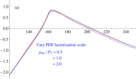
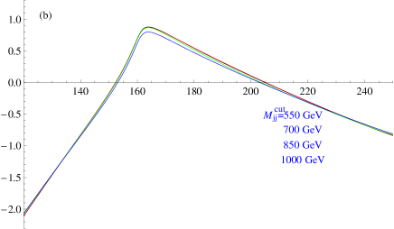
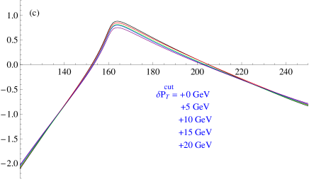
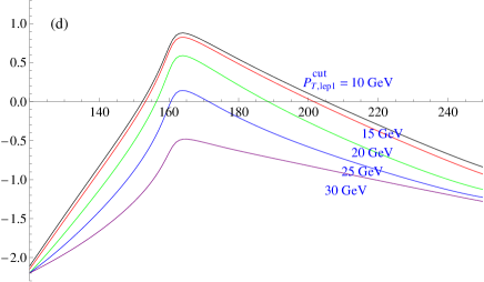
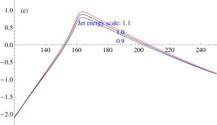
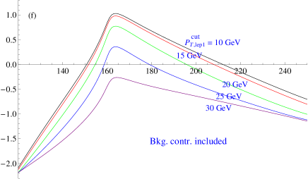
Figure 5: $10^{5}\times\langle{\cal O}_{G}\rangle$ vs. $m_{H}$ (parameter in $d\Gamma_{H\to\ell\ell\nu\nu}/dE_{0}|_{M_{\ell\ell}<45{\rm GeV}}$). MC events with $m_{H}^{\rm MC}=150$ GeV and for $\mu\mu$ mode are used. Through (a)–(e) only the signal events are used, while in (f) both signal and background events are used. All the cut values, except the ones shown explicitly in figs. (b)(c)(d)(f), are kept fixed to their default values.

Now we examine stability and reliability of our prediction, using the $\mu\mu$ mode and MC input $m_{H}^{\rm MC}=150$ GeV. In Fig. 5(a) we vary the factorization scale $\mu_{\rm fac}$ in PDF and PYTHIA and plot $\langle{\cal O}_{G}\rangle$ as a function of $m_{H}$: $\mu_{\rm fac}$ is taken as $1/2$, $1$ and $2$ times its default value of MadEvent ($P_{T}$ of each scattered parton from each proton in the vector-boson fusion case). $\delta m_{H}$ (and hence the value of $m_{H}$ where $\langle{\cal O}_{G}(m_{H})\rangle$=0) changes by about 0.8 GeV as $\mu_{\rm fac}$ is varied from $1/2$ to 2. In Fig. 5(b) we vary the cut value of the invariant mass of tagged two jets from 550 GeV to 1 TeV. Corresponding variation of $\delta m_{H}$ is about 0.8 GeV. In Fig. 5(c) we vary the values of the $P_{T}$ cuts of tagged jets, $P_{T,j1}>40~{}{\rm GeV}+\delta P_{T,j}$ and $P_{T,j2}>20~{}{\rm GeV}+\delta P_{T,j}$, between $\delta P_{T,j}=0$ and 20 GeV. ($\delta P_{T,j}=0$ is the default value.) Variation of $\delta m_{H}$ is about 1.0 GeV. These features agree with our expectation that $m_{H}$ determination is insensitive to PDF and cuts involving only jets, since only the $\beta$ distribution of the Higgs boson would be affected. Moreover, we find that $\langle{\cal O}_{G}\rangle$ as a function of $m_{H}$ is also fairly stable.

On the other hand, $\delta m_{H}$ and $\langle{\cal O}_{G}(m_{H})\rangle$ depend strongly on the lepton cuts. In Fig. 5(d) we vary the values of the $P_{T}$ cut of the leading muon between 10 GeV and 30 GeV (while keeping the $P_{T}$ cut value of the subleading muon to 10 GeV). The line $\langle{\cal O}_{G}(m_{H})\rangle$ moves downwards and changes shape as the cut becomes tighter. This stems from the fact that the $P_{T}$ cut suppresses lower part of the lepton energy distribution.

Cuts involving missing transverse momentum $\vec{P}_{T}^{\rm miss}$($=-\vec{P}_{T}^{\rm had}-\vec{P}_{T}^{\ell\ell}$) may also affect the $m_{H}$ determination, since the cuts affect the lepton energy distribution through indirect restrictions on $\vec{P}_{T}^{\ell\ell}$. Here, $\vec{P}_{T}^{\ell\ell}$ denotes the transverse momentum of the tagged dilepton system, while $\vec{P}_{T}^{\rm had}$ denotes the sum of the transverse momenta of all other visible particles. Since magnitudes of systematic uncertainties in $\vec{P}_{T}^{\rm had}$ and $\vec{P}_{T}^{\ell\ell}$ measurements are rather different, instead of varying cuts involving $\vec{P}_{T}^{\rm miss}$, we multiply $|\vec{P}_{T}^{\rm had}|$ by a scale factor of 0.9, 1.0 and 1.1; we keep all the cut values unchanged. See Fig. 5(e). This variation of energy scale affects restrictions on $\vec{P}_{T}^{\ell\ell}$ indirectly, since bounds on $\vec{P}_{T}^{\rm miss}=-\vec{P}_{T}^{\rm had}-\vec{P}_{T}^{\ell\ell}$ are kept fixed. We find that variation of $\delta m_{H}$ is about 1.6 GeV.

In Fig. 5(f) we include the background contributions and vary the leading lepton $P_{T}$ cut. (Through Fig. 5(a)–(e) only leptons from the signal events are used.) Compared to Fig. 5(d), each line moves upwards and the line shape is modified slightly by inclusion of the backgrounds. We have already seen this effect in the shift of the reconstructed Higgs mass in Fig. 4 and Tab. 2.

From these examinations and similar examinations for other input Higgs mass values and decay modes, we estimate that our prediction is fairly insensitive to uncertainties in PDF and jet variables. On the other hand, the prediction is strongly dependent on the lepton $P_{T}$ cuts. It is dependent also on other lepton acceptance corrections. These effects with respect to only leptons can in principle be estimated accurately, by understanding detector coverage and detector performances well.

We note that all the lines in Fig. 5(f) can be plotted using the real experimental data and can be compared with the prediction. Since these lines can be predicted accurately and are dependent on MC input Higgs mass value $m_{H}^{\rm MC}$, we can determine the Higgs mass by a fit of $\langle{\cal O}_{G}(m_{H})\rangle$, provided the background contributions can be estimated accurately. Similarly, all the lines in Figs. 5(b) and (c) can be compared, after inclusion of background contributions, with the corresponding ones plotted using the real experimental data. Alternatively we may make similar comparisons by loosening various cuts. This procedure raises relative weight of background contributions, so that we can test the prediction for the background contributions. We may also make use of the large degree of freedom of the observable ${\cal O}_{G}$ for further tests of the prediction.

In the case that higher lepton $P_{T}$ cuts are unavoidable, determination of the Higgs mass by a fit of $\langle{\cal O}_{G}(m_{H})\rangle$ would be more realistic, as mentioned above, since $\langle{\cal O}_{G}(m_{H})\rangle$ is shifted considerably. Explicitly, a fit can be carried out in the following way. We can compute $\langle{\cal O}_{G}(m_{H})\rangle$ using lepton energy distributions measured in a real experiment and MC simulation, respectively, as

$$\langle{\cal O}_{G}(m_{H})\rangle_{\rm exp}\equiv\int dE_{\ell}\,D_{\rm exp}(E_{\ell};m_{H}^{\rm true}){\cal O}_{G}(E_{\ell};m_{H}),$$ (7)

$$\langle{\cal O}_{G}(m_{H})\rangle_{\rm MC}\equiv\int dE_{\ell}\,D_{\rm MC}(E_{\ell};m_{H}^{\rm MC}){\cal O}_{G}(E_{\ell};m_{H}).$$ (8)

Defining a distance between $\langle{\cal O}_{G}(m_{H})\rangle_{\rm exp}$ and $\langle{\cal O}_{G}(m_{H})\rangle_{\rm MC}$ as

$$d^{2}(m_{H}^{\rm MC})\equiv\int_{m_{1}}^{m_{2}}\!\!\!\!dm_{H}\,w(m_{H})\,$$

$$~{}~{}~{}~{}~{}~{}~{}~{}~{}~{}~{}~{}~{}~{}~{}\times[\langle{\cal O}_{G}(m_{H})\rangle_{\rm exp}-\langle{\cal O}_{G}(m_{H})\rangle_{\rm MC}]^{2}\,,$$ (9)

and minimizing $d(m_{H}^{\rm MC})$, we may reconstruct the Higgs mass. Here, $w(m_{H})\geq 0$ denotes an appropriate weight. As the lepton $P_{T}$ cuts become tighter, sensitivity to the Higgs mass decreases. For instance, in the case $m_{H}^{\rm true}=150$ GeV, if we impose $P_{T,{\rm lep1}}>25$ GeV and $P_{T,{\rm lep2}}>10$ GeV to the leading and subleading leptons, respectively, we estimate that the statistical error of the Higgs mass, reconstructed by the above fit, to be about $5.0$ GeV for an integrated luminosity of 100 fb^-1. The size of error is not very dependent on choices of $m_{1}$ and $m_{2}$ or the weight $w$. (We took $m_{1}=120$ GeV, $m_{2}=240$ GeV and $w=1$.)

Comparing Tab. 3 and the examination in Figs. 5, we anticipate that the statistical error will dominate over systematic errors. The accuracy of $m_{H}$ determination is better for a lighter Higgs mass, within the range $150~{}{\rm GeV}\hbox{ \raise 3.0pt\hbox to0.0pt{$<$}\raise-3.0pt\hbox{$\sim$} }m_{H}\hbox{ \raise 3.0pt\hbox to0.0pt{$<$}\raise-3.0pt\hbox{$\sim$} }200$ GeV. (e.g. If $m_{H}=150$ GeV, it would be reconstructed with 2–3% accuracy with 100 fb^-1 integrated luminosity.)

Let us comment on the effects of leptons from $\tau$’s, which we have neglected. Since these leptons would have a lower energy spectrum, the effects of the lepton $P_{T}$ cuts are likely to be enhanced. We anticipate from Fig. 5(d) that the effects are to move the line $\langle{\cal O}_{G}(m_{H})\rangle$ downwards. Nevertheless, we expect that the additional contribution from $\tau$’s and the cut effect will be accurately predictable and should not deteriorate the $m_{H}$ determination.

The main purpose of the present study on $m_{H}$ reconstruction is to demonstrate that the mass reconstruction using ${\cal O}_{G}$ is applicable to such a complicated process. We chose the $WW$–fusion mode (rather than $gg$–fusion mode) since a good signal-to-noise ratio is beneficial in demonstrating clearly the characteristics of the present method. We confirmed stability of our prediction except against purely leptonic cuts. Good understanding of background contributions is also important.

Experimentally $m_{H}$ would be reconstructed very accurately using the decay modes $H\to ZZ^{(*)}\to\ell\ell\ell\ell$ in the relevant mass range Ball:2007zza . The $WW^{(*)}$ decay modes can be used to test consistency of the Higgs mass values, using our method or those of Davatz:2006ja ; Barr:2009mx . Ref. Davatz:2006ja uses leptonic variables but depends severely on PDF. We reemphasize that our method is independent of PDF in the leading-order. In a future work, we may examine the $gg$–fusion mode, in which the statistical error would be smaller while systematic errors would be larger than the $WW$–fusion mode.

The observables proposed in this paper would have wide applications. For example, in supersymmetric models, ${\cal O}_{G}$ can be applied to a slepton decay into a lepton plus an undetected particle; since it is a two-body decay, its analysis would be straightforward. Another possible application is a measurement of the top quark mass. A preliminary analysis indicates that the top quark polarization effects are small.

The authors express their condolences for victims of disasters in Japan. The disasters also struck the current project heavily. The authors hope the completion of this work to be a step forward in revival from the tragedy. The work of Sumino is supported in part by Grant-in-Aid for scientific research No. 23540281 from MEXT, Japan.

References

- (1) A. Barr, C. Lester and P. Stephens, J. Phys. G 29, 2343 (2003); W. S. Cho, K. Choi, Y. G. Kim, C. B. Park, Phys. Rev. Lett. 100, 171801 (2008). W. S. Cho, K. Choi, Y. G. Kim, C. B. Park, Phys. Rev. D79, 031701 (2009); M. Burns, K. Kong, K. T. Matchev, M. Park, JHEP 0810, 081 (2008).
- (2) A. J. Barr and C. G. Lester, J. Phys. G 37 (2010) 123001.
- (3) F. Maltoni and T. Stelzer, JHEP 0302 (2003) 027; J. Alwall et al., JHEP 0709 (2007) 028; J. Alwall et al., JHEP 1106, 128 (2011).
- (4) T. Sjostrand, S. Mrenna and P. Skands, JHEP 0605 (2006) 026.
- (5) http://www.physics.ucdavis.edu/~conway/research/ software/pgs/pgs4-general.htm.
- (6) S. Asai et al., Eur. Phys. J. C32S2, 19-54 (2004).
- (7) http://www.tifr.res.in/~lp11.
- (8) T. Aaltonen et al., arXiv:1103.3233 [hep-ex].
- (9) ATLAS Collaboration, ATLAS-CONF-2011-134, http://cdsweb.cern.ch/record/1383837/files/ATLAS-CONF-2011-134.pdf.
- (10) G. L. Bayatian et al., J. Phys. G 34, 995 (2007).
- (11) G. Davatz, M. Dittmar and F. Pauss, Phys. Rev. D 76 (2007) 032001.
- (12) A. J. Barr, B. Gripaios, C. G. Lester, JHEP 0907, 072 (2009); K. Choi, S. Choi, J. S. Lee, C. B. Park, Phys. Rev. D80, 073010 (2009).