Emission Measure Distribution and Heating of Two Active Region Cores

Abstract

Using data from the Extreme-ultraviolet Imaging Spectrometer aboard Hinode, we have studied the coronal plasma in the core of two active regions. Concentrating on the area between opposite polarity moss, we found emission measure distributions having an approximate power-law form EM$\propto T^{2.4}$ from $\log\,T=5.5$ up to a peak at $\log\,T=6.55$. We show that the observations compare very favourably with a simple model of nanoflare-heated loop strands. They also appear to be consistent with more sophisticated nanoflare models. However, in the absence of additional constraints, steady heating is also a viable explanation.

1 Introduction

It has proved very challenging to obtain definitive answers to the very stubborn problem of how the solar corona is heated. The heating of warm ($\sim 1$ MK) coronal loops is one exception. There is now widespread agreement, though not complete consensus, that these are multi-stranded structures heated impulsively by storms of nanoflares (e.g., Klimchuk 2006, 2009 and references cited therein). Warm loops account for only a fraction of the coronal plasma, however. The corona also contains hot ($>2$ MK) loops and diffuse emission at all temperatures. Much recent attention has focused on what is often called the ”hot core” of active regions. This is the subject of our study reported here.

A fundamental question concerns the temporal nature of coronal heating. This is often discussed in terms of a dichotomy between steady heating and nanoflares. What really matters for determining the properties of the coronal plasma is the heating on individual magnetic flux strands (field lines). Few, if any, serious coronal heating theories predict that the energy release is steady in this regard (Klimchuk, 2006); rather, the heating occurs in short-lived bursts. We refer to these small-scale impulsive bursts as nanoflares. No particular physical mechanism is implied by the term. It could be magnetic reconnection in tangled magnetic fields as envisioned by Parker (1983) and probably involving the secondary instability of current sheets (Dahlburg, Klimchuk, & Antiochos, 1995); it could be wave dissipation in drifting resonance layers (Ofman, Klimchuk, & Davila, 1998); or it could be another mechanism altogether.

An important parameter is the time delay between successive nanoflares on a given strand. By delay we mean the time interval between the end of one nanoflare and the start of the next. If the delay is much shorter than a cooling time (tens to hundreds of seconds) then there is minimal cooling between events and the heating is effectively steady. We can approximate such a situation with perfectly steady heating. It is becoming more common for the term ”steady heating” to imply nanoflares that repeat with a high enough frequency that the temperature hovers around one value and for ”nanoflare heating” to imply nanoflares that repeat with a low enough frequency that the plasma cools substantially. In addition, ”nanoflare heating” usually implies heating that takes place in the corona. Impulsive energy release in the chromosphere that is associated with spicules (De Pontieu et al., 2011) is a different phenomenon, though it might have similar physical attributes.

Attempts to determine whether active region cores have steady or nanoflare heating have been inconclusive. Some studies point out that the intensities, electron densities, Doppler shifts, and nonthermal broadening of observed emissions are often quite steady in the sense that fluctuation amplitudes are small (Antiochos et al., 2003; Tripathi et al., 2010; Brooks and Warren, 2009). A reasonable conclusion is that the heating is steady. However, this is only certain if the cross-field spatial scale of the heating is comparable to or larger than the resolution of the observations (typically about 1000 km). There is good reason to believe that the coronal magnetic field is structured on a much smaller scale (Klimchuk, 2006) and so it seems likely that the heating is also structured on a much smaller scale. If so, direct evidence of nanoflares would be washed out, since the emission from many different strands would be averaged together. Such averaging occurs both across the observational pixel and along the optically thin line of sight. Hence, steady intensities, densities, Doppler shifts, and nonthermal broadening are consistent with both steady heating and nanoflare heating. We note also that subtle variability in seemingly steady intensities can provide good evidence for nanoflares (Terzo et al. 2011; Viall & Klimchuk 2011b).

Faced with the likelihood of unresolved structures, we must look to other ways of distinguishing between steady and impulsive heating. Investigating the distribution of plasma with temperature, as quantified in the the emission measure distribution, EM($T$), is one promising approach. There have been many determinations of EM($T$) through the years, but they have tended to average over large areas. Results reported for active regions generally obey the power law EM($T$) $\propto T^{b}$ up to a peak near 3 MK, where the index $b$ ranges between 1 and 3 (e.g., Dere 1982; Dere & Mason 1993; Brosius et al. 1996). When plotted on a log-log scale, $b$ is the slope of a straight line. Some authors use the differential emission measure, DEM($T$), which is related to the emission measure by EM($T$) = $T\times$ DEM($T$). The slope of DEM($T$) is smaller by an amount 1.0.

Observations that average over large areas tend to include both coronal and transition region emissions. Transition region here refers not to a particular temperature range, but rather to the thin region of steep temperature gradient at the base of the corona. As a rule of thumb, the temperature of the top of the transition region is about 60% of the maximum temperature in the strand (Klimchuk et al., 2008; Bradshaw & Cargill, 2010). The transition region can therefore reach very high temperatures depending on how hot the strand is. Million degree moss seen in the 171 channels of SOHO/EIT, TRACE, and SDO/AIA is just the transition region footpoints of hot core strands. We use this later to determine the width of the core in the active region we investigate here. Moss can tell us a great deal about the core plasma. For example, in a recent paper we showed that the EM distribution of moss is better explained if the core is heated impulsively than in a steady fashion (Tripathi, Mason, & Klimchuk, 2010). Our results are compatible with steady heating if the cross sectional area has the proper temperature dependence in the transition region ”throat” of a rapidly expanding strand, but we argued that this temperature dependence is not likely to be maintained in the presence of spatial and temporal pressure nonuniformities across the moss.

Two recent studies have explicitly avoided moss and concentrated on the coronal emission in the cores of active regions. Warren et al. (2011) studied a small ($10\times 15$ arcsec²) inter-moss region between opposite magnetic polarities and found an emission measure distribution that can be approximated by EM $\propto T^{3.26}$ in the range $6.0\leq\log\,T\leq 6.6$. The EM is 400 times smaller at $\log\,T=5.8$ than it is at $\log\,T=6.6$. Winebarger et al. (2011) averaged over a $5\times 25$ arcsec² inter-moss area from another active region and found a similar power-law slope ($EM\propto T^{3.2}$) over the range $6.0\leq\log\,T\leq 6.5$. These distributions are considerably steeper than what has been published in the past. Is this because the previous studies averaged over a mixture of different features (core, moss, non-core loops, etc.), or is it because the inter-moss regions of the two new studies are, by chance, not typical of core plasma in general?

To help answer this question, we have analyzed four inter-moss regions within active region AR 10961 that was observed by multiple spacecraft and one small inter-moss region in active region AR 10980. In the next sections, we describe the observations and our analysis of the data. We derive emission measure distributions for the inter-moss regions, and by estimating the plasma in the foreground of the core, we determine the EM distribution of the core plasma itself. We then discuss the results in the context of related measurements and the predictions of steady and nanoflare heating.

2 Observations and Data Analysis

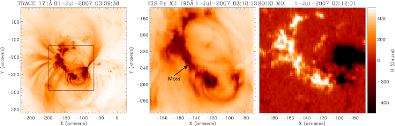
Figure 1: Left panel: TRACE 171 Å image showing the complete active region. The over-plotted box shows the EIS field of view. Middle panel: An EIS image obtained in Fe XII 195.12 Å. The arrow identifies the moss. Right Panel: Co-aligned magnetogram obtained by the MDI instrument on SOHO. The left and middle panels are displayed in negative intensities.

On July 01, 2007, the Extreme-ultraviolet Imaging Spectrometer (EIS; Culhane et al., 2007) obtained a full spectral scan of the active region AR 10961 with an exposure time of 25 sec using its 1″ slit. The field of view of the raster was 128″ by 128″ which basically covered most of the active region. The EIS raster started at 03:18:13 UT and finished at 04:14:53 UT. A full spectral scan of the active region was telemetered which allowed us to choose spectral lines formed over a broad range of temperature from $\log\,T=5.5$ (Mg V) to $\log\,T=6.75$ (Fe XVII, identified by del Zanna & Ishikawa (2009) in EIS spectra). Table 1 lists all the spectral lines used in this study. The left panel in Fig. 1 shows the active region recorded by the Transition Region And Coronal Explorer (TRACE; Handy et al., 1999) in the 171 Å bandpass. The over-plotted box marks the region which was rastered by EIS. An EIS image obtained in Fe XII $\lambda$195.12 Å is shown in the middle panel of Fig. 1. The arrow identifies the moss. The right panel shows a co-aligned magnetogram obtained by the MDI instrument on SOHO. As can be seen in Fig. 1, the brightest moss regions show a strong correlation with the following positive magnetic polarity (cf. Tripathi et al., 2008; Noglik et al., 2009). There also appears to be some weak moss associated with the leading negative magnetic polarity. We also note that most of the core loops connect the brightest moss regions to the negative polarity penumbra of the sunspot.

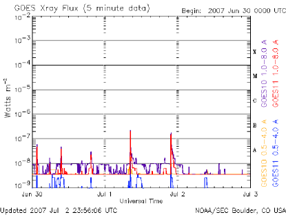
Figure 2: GOES X-ray profile from June 30th to July 2nd 2007 showing minimal activity.

This active region raster is ideal for our study as it does not show any flaring activity during the EIS raster. This is essential for our study because we are mainly interested in the thermal structure of quiescent active regions. Fig. 2 displays the GOES X-ray flux for three days from June 30, 2007. It is clear from the plot that the activity remains minimal for three days except two small B-class flares observed on July 1, 2007. However, both the flares occurred after the EIS raster studies were completed.

The full spectral scan with a good exposure time allowed us to choose spectral lines formed over a broad range of temperatures in order to study the emission measure distribution of the plasma along the line of sight (LOS) in the core the active region. For this purpose we have selected relatively unblended lines (see Table 1) from the spectrum which covers a temperature range of $\log T[\mathrm{K}]=5.5\mbox{--}6.8$. We have used the standard EIS software provided in SolarSoft to process the data and eis_auto_fit, also provided in SolarSoft, for Gaussian fitting the spectral lines. For de-blending some of the blended lines, we have used the same procedure as in Tripathi et al. (2010) based on the recommendations of Young et al. (2007, 2009). For visual inspection, we have also used data recorded by the TRACE and X-Ray Telescope (XRT, Golub et al., 2007) on July 01, 2007 of the AR 10961. We have used standard software provided in SolarSoft for processing these data.

3 Visual Inspection of Hot and Warm Emission in the Core of the Active Region

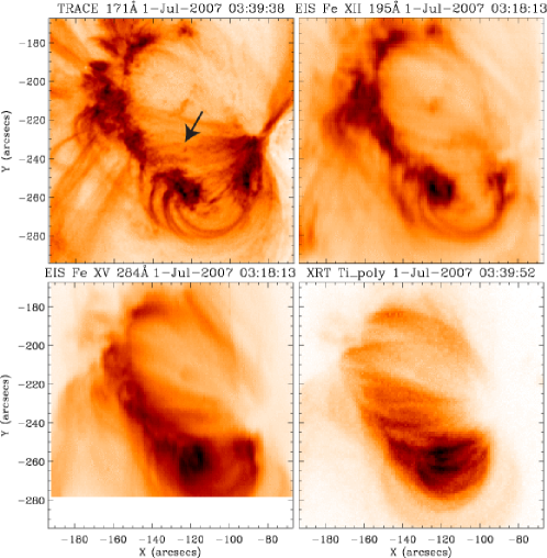
Figure 3: Co-aligned TRACE 171Å (top left), EIS Fe XII 195Å (top right), EIS Fe XV 284Å (bottom left) and XRT Ti_ploy image shown in negative intensities taken on July 01, 2007. Images are displayed in negative colors. The arrow in the top left image labels the loop-like warm emission in the core of active regions.

We have analysed the images recorded by TRACE and XRT in conjunction with the images obtained from the EIS raster. Figure 3 displays co-aligned images from TRACE 171Å (top left), EIS Fe XII 195Å (top right), EIS Fe XV 284Å (bottom left), and XRT using the Ti_poly filter (bottom right). The TRACE and XRT images were taken when the EIS slit was near the middle of the raster. We used EIS Fe XII 195Å and Si X 261Å images to co-align the data taken by the two different CCDs of EIS. The TRACE image was then co-aligned with EIS Fe XII image and the XRT image was co-aligned with EIS Fe XV image. We believe that the co-alignment achieved is quite accurate with an error of about 3-5 arcsec. The images are displayed in negative intensities.

The figure clearly shows that both hot and warm emission exists in the core of the active region. The emission consists of both a diffuse component and distinct loops (labeled by an arrow in the TRACE 171 image). It is not generally appreciated that the diffuse component usually dominates the signal from active regions. Identifiable loops are typically just modest enhancements on a smoothly varying background (e.g., del Zanna & Mason, 2003; Viall & Klimchuk, 2011a). The loops are not as distinctive in the EIS images in part because of the lower spatial resolution of the observations and in part because hotter emission is inherently more fuzzy (Tripathi et al., 2009; Guarrasi, Reale, & Peres, 2010). We note here that TRACE images obtained before and after the EIS raster show that strong warm emission is always present in the core of the active region.

4 Emission Measure Distribution in Inter-moss Regions

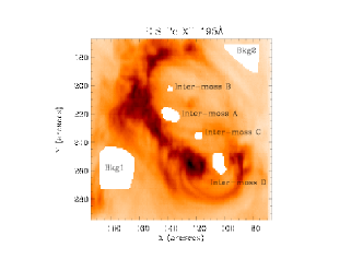
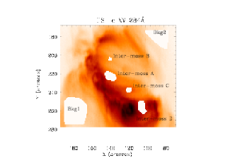
Figure 4: Fe XII(left) and Fe XV images showing the four inter-moss regions, labelled as A, B, C and D and the background regions labelled as Bkg1 and Bkg2 chosen for the study.

In order to determine the temperature distribution of the coronal plasma within the core, we have performed an emission measure (EM) analysis of three different inter-moss regions, labeled A ($\sim 15\times 10$ arcsec²), B ($\sim 5\times 5$ arcsec²), and C ($\sim 7\times 7$ arcsec²) in Figure 4. The inter-moss regions are clearly separated from both the bright moss seen in the TRACE 171 image and the strong magnetic fields seen in the magnetogram. They are spaced along the axis of a magnetic arcade that spans the neutral line, connecting opposite polarities. Regions B and C were chosen to be small to be sure that their EM distributions reflect the distribution of strands of different temperature (one temperature per strand) and not the variation of temperature along each strand. Because we sample three regions, rather than averaging over one large area, we can be confident that our results are not strongly biased by a small but exceptionally bright feature.

Although the three regions are all classified as inter-moss, they appear quite different from each other in the images of Fig. 3. The emission seems to become brighter with more evidence of distinct loop structures in progressing from north to south (i.e., from B to A to C). This could suggest substantially different physical characteristics. However, we will show that the plasma is in fact very similar in all three regions. This illustrates how deceiving images can be when treated subjectively. Meaningful conclusions can only be drawn from a quantitative analysis of the data. Table 1 presents the average intensities of regions A, B, and C together with their 1-sigma errors obtained from Gaussian fitting for the 24 EIS spectral lines used in our study. We also note that there is a systematic uncertainty of 22% in intensities due to radiometric calibration as was measured by Lang et al. (2006).

We derive EM distributions from the intensities using the method proposed by Pottasch (1963). For each spectral line, the EM at the peak formation temperature, $T_{\rm max}$, is approximated by assuming that the contribution function is constant and equal to its average value over the temperature range $\log\,T_{\rm max}-0.15$ to $\log\,T_{\rm max}+0.15$ and zero at all other temperatures. We assume the ionization equilibrium values of Dere et al. (2009) as given in Chianti v.6.01 (Dere et al., 1997, 2009), and we consider both photospheric (Grevesse and Sauval, 1998) and coronal (Feldman, 1992) abundances.

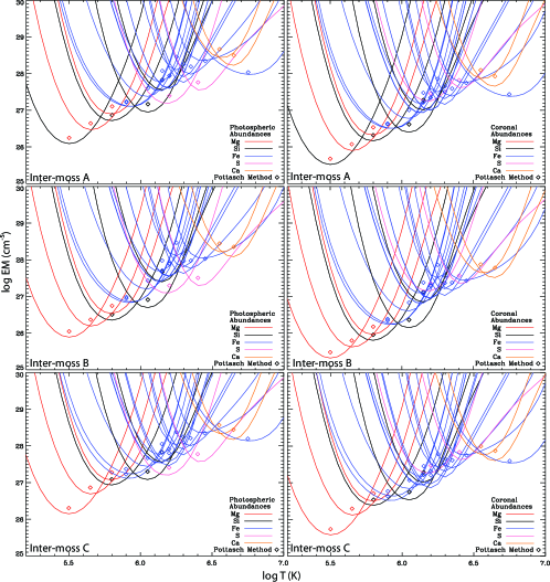
Figure 5: EM loci plots (inverted ’U’ curves) and emission measure derived using Pottasch method (diamonds) of each spectral lines for the three inter-moss regions labelled A, B and C in Fig. 4. The plot is color coded for different elements.

The resulting EM values are plotted as diamonds in Figure 5. The top, middle, and bottom panels are for regions A, B, and C, respectively. Panels on the left use photospheric abundances and those on the right use coronal abundances. Coronal abundances provide more consistent results (i.e., less scatter in the data), and so we conclude that they are more appropriate. Warren et al. (2011) reached the same conclusion for the inter-moss region they studied. Differences in the results obtained with coronal and photospheric abundances are rather small, however, as all lines with the exception of two sulphur lines come from low-FIP (first ionization potential) elements. The figure is color coded for the different elements. Sulphur is pink, and its two lines fall at $\log\,T=6.20$ and $6.40$. We will assume coronal abundances for the remainder of the paper. It is interesting to note, however, that moss observations of this active region are more consistent with photospheric abundances (Tripathi, Mason, & Klimchuk, 2010).

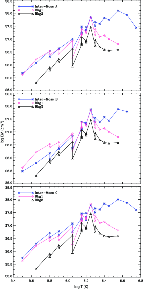
Figure 6: Emission measure distribution in Inter-moss regions A, B and C over-plotted with the EMs of two background regions namely Bkg 1 and Bkg 2 labelled in Fig. 4.

The inverted ”U” curves in the figure are EM loci plots (see del Zanna, Landi, & Mason, 2002, and references therein for details on EM loci). Each curve gives the amount of emission measure that would be needed to produce the observed line intensity if the plasma were isothermal at the indicated temperature. The curves have their minimum at the temperature where the Pottasch value is plotted, as this is where the line emits most efficiently and therefore requires the least emission measure. As expected, the Pottasch values lie slightly above the EM loci curves. It is clear that the Pottasch method gives good results for the actual emission measure distribution that produces the observed line intensities. Were this not the case, the Pottasch values would deviate significantly from the envelope of the EM loci curves. Henceforth, we use the terms EM distribution and EM curve interchangeably to describe the connected Pottasch values. They are shown in blue with asterisks in Figure 6.

We estimate that the total uncertainty in the derived EM values is approximately 50%. This includes errors resulting from photon counting statistics, approximate atomic physics, uncertain elemental abundances, and limitations in the Pottasch method. The corresponding error bars in Figure 6 are $\Delta\log$ EM $\approx\pm 0.2$.

The EM curves for all three inter-moss regions are very similar. To within the uncertainties, they increase monotonically with temperature from $\log\,T=5.5$ to a maximum at $\log\,T=6.55$. From a simple linear fitting to this range we find that EM($T$) $\propto T^{b}$ with slope $b=2.33\pm 0.15$, $2.47\pm 0.22$, and $2.08\pm 0.14$ for regions A, B, and C, respectively. The ratio of the EM at $\log\,T=6.55$ to $\log\,T=5.8$ is 45, 62, and 23, where we have used the actual values at these temperatures and not the linear fit. Since we have two spectral lines at $\log\,T=5.8$, namely Si VII and Mg VII, we have taken the average of two EM values before obtaining the ratio. Although there is more plasma at higher temperatures, it is clear that a substantial amount of plasma is present at all temperatures along the LOS.

In addition to having similar slope, the EM curves for the three inter-moss regions have similar magnitude. As already mentioned, this contradicts the erroneous impression of greatly different brightness that one gets from simply looking at the images in Fig. 3. Such impressions have in the past led to the incorrect notion that warm plasma exists primarily outside of the core of active regions. In fact, warm emission is usually stronger in the core than outside (Viall & Klimchuk, 2011a).

Not all of the line emission used to generate the inter-moss EM curves in Figure 5 comes from the core proper. Some of it comes from foreground plasma that is part of the higher arching field that overlies the core. To estimate the contribution from this foreground we generate EM curves for two ”background” regions located outside of the moss, shown labeled as Bkg 1 and Bkg 2 in Figure 4. The term background is something of a misnomer in this case. As we discuss shortly, the EM of the foreground to the core will be less than that of the background regions.

The EM curves of the two background regions are shown repeated in the three panels of Figure 6. Bkg 1 is indicated by pink diamonds, and Bkg 2 is indicated by black triangles. The background curves have a similar shape to the inter-moss curves up to $\log\,T=6.2$, and then they decrease at higher temperatures. The magnitude is comparable to the inter-moss regions for Bkg 1 and roughly a factor of 3 smaller for Bkg 2. The TRACE 171 image in Figure 1 reveals that Bkg 1 contains distinctive fan loops that have a southward trajectory and do not seem to overlie the core. For this reason, we suggest that Bkg 2 is a more appropriate indicator of the foreground plasma.

The EM of both background regions very likely over-estimates the EM of the foreground plasma. Emission from the background regions is integrated along the full line of sight from the solar surface to the observer, whereas the foreground plasma begins at the top of the core arcade. Since lower-lying plasma is denser and brighter due to gravitational stratification, the difference in the integration is substantial. We estimate the difference by considering a vertical column of plasma with a density scale height $H_{n}$. It is easy to show that the ratio of the integrated EM above height $z$ to the integrated EM above the photosphere ($z=0$) is

$$\frac{EM(z)}{EM(0)}=\exp\left(-\frac{2z}{H_{n}}\right).$$ (1)

If we take $z$ to be the height of the core arcade, equation 1 is the amount by which the background EM must be reduced to obtain a proper estimate of the foreground. We estimate from the moss in Fig. 3 that the arcade width is approximately 80 arcsec, or $6\times 10^{4}$ km. Assuming that the arcade is semi-circular, its height is then $3\times 10^{4}$ km. TRACE 171 emission is formed near $\log\,T=5.8$, for which the gravitational scale height is $3\times 10^{4}$ km. Taking this for $H_{n}$, we obtain a reduction factor of 0.14 from equation 1. This is only a lower limit, however, as distinguishable warm loops are known to have a density scale height that is larger than hydrostatic by up to a factor of 2 (Aschwanden et al., 2001). If the diffuse component of the warm emission also behaves in this way, so that $H_{n}=6\times 10^{4}$ km, then the reduction factor could be as large as 0.4.

Summarizing, we conclude that the foreground plasma accounts for between 5 and 40% of the inter-moss emission measure at $\log\,T=5.8$. The low extreme corresponds to Bkg 2 with a reduction factor of 0.14, and the high extreme corresponds to Bkg 1 with a reduction factor of 0.4. As discussed above, we believe that Bkg 2 is more representative of the foreground plasma, and therefore the lower part of the range seems more likely. We conclude that the inter-moss EM curves of Figure 6 (blue asterisks) are largely indicative of core plasma and not greatly contaminated by foreground plasma. Figure 8 shows our best estimate of a representative EM curve for the core itself. The data points are the averages of regions A, B, and C (linear averages, not logarithmic) minus the averages of regions Bkg 1 and Bkg 2 reduced by a factor of 0.25. The curve has a slope of approximately 2.4.

Although we believe our approach to estimating the foreground emission is very sensible, we acknowledge that this is a very difficult task and that the uncertainties may be large. Therefore, in addition to what we take as the optimum foreground subtraction described above (subtracting the average emission from Bkg1 and Bkg2 reduced by a factor of 0.25), we also consider two additional possibilities. The first is no foreground subtraction, as presented earlier. The second is a severe foreground subtraction, where we subtract the full emission from region Bkg 2 without a reduction factor. The resulting best-fit slopes for the range $5.8\leq\log\,T\leq 6.55$ are given in Table 2. The slopes turn out to be largely independent of how the foreground is estimated.

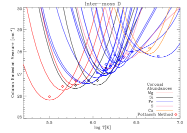
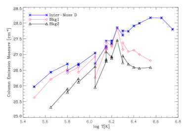
Figure 7: Left panel: EM loci plots (inverted ’U’ curves) and emission measure derived using Pottasch method (diamonds) of each spectral line for inter-moss region D labelled in Fig. 4. Right Panel: Emission measure distribution in Inter-moss region D over-plotted with the EMs of two background regions namely Bkg 1 and Bkg 2 labelled in Fig. 4.

We examined a fourth region, labeled D in Figure 4. It includes the brightest XRT emission that does not directly overlie strong photospheric field. We tentatively identify this as an inter-moss region. However, because the corridor between opposite polarity strong field is so narrow ($<$ 10 arcsec), we cannot be certain that there is no contamination from footpoint emission. The EM loci curves and EM distribution for region D are shown in Figure 7. They have a similar appearance to those for regions A, B, and C. The slopes obtained with the different foreground subtractions are given in Table 2. They are similar to the slopes for regions A, B, and C. The emission measure is 37 times smaller at $\log\,T=5.8$ than it is at $\log\,T=6.55$ (with no foreground subtraction).

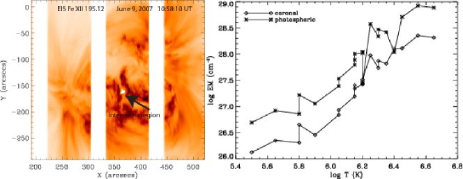
Figure 9: Left panel: Fe XII image obtained from EIS raster on June 9, 2007. The arrow shows the inter-moss region chosen to study the EM distribution. Right panel: Emission measure distribution obtained for the inter-moss region shown in the left panel.

We studied a second active region, AR 10980, though in less detail. It was observed by EIS on June 9, 2007 at 10:58:10 UT. Figure 9 shows the Fe XII 195.12 image (left panel) and EM curves (right panel) obtained for the inter-moss region ($\sim 10\times 10$ arcsec²) labeled on the left. Again, coronal abundances provide a more consistent result. Without foreground subtraction, the emission measure approximately follows a power law of slope 2.33$\pm$0.19 up to a maximum at $\log\,T=6.55$. The EM is 69 times smaller at $\log\,T=5.8$ than it is at $\log\,T=6.55$.

The slopes given in Table 2 are generally similar to those reported previously for many other active regions, although they are toward the steep end of the published range of 1–3 (e.g., Dere 1982; Dere & Mason 1993; Brosius et al. 1996). We must remember, however, that those earlier studies may include moss and other non-core plasma. O’Dwyer et al. (2011) studied an active region at the limb and found very flat EM curves between $\log\,T=6.0$ and $6.5$. Those observations do not include moss, but they do include non-core plasma along the horizontal line of sight.

A more relevant comparison is with the recent studies of Warren et al. (2011) and Winebarger et al. (2011), which also concentrate on inter-moss regions. The considerably steeper slopes of 3.26 and 3.2 found by Warren et al. (2011) and Winebarger et al. (2011) are from temperature ranges of $6.0\leq\log\,T\leq 6.6$ and $6.0\leq\log\,T\leq 6.5$, respectively. To make a more direct comparison with their results, we have redone our analysis for the range $6.05\leq\log\,T\leq 6.55$. Since Warren et al. subtracted no foreground before making their measurements and Winebarger et al. subtracted only a weak foreground (Winebarger 2011, private communication), the most appropriate comparison is with ”No Foreground”.

The new slopes which we found for this temperature range vary from 1.75 to 3.05 (including estimated error) when no foreground emission is subtracted. When foreground is subtracted, both optimum and severe, the values range from 1.95 to 3.15 (including estimated errors). Region D and AR10980 have the steepest slopes. It should be noted that the values found in the other studies are steeper than the slopes we found in all cases, indeed they are beyond the extreme limit of our values.

The fact that the slopes change depending on the width of the temperature fitting range indicates that the assumption of a single power law is not strictly valid. Further analysis is required to determine how the assumption fails. Do broken power laws apply, and if so, where are the breaks? Is any range suitably approximated by a power law? We suggest that choosing the maximum of EM($T$) as the high-temperature end of the fitting range may be dangerous, since the distribution is likely to roll over near the maximum rather than having a sharp peak.

We stress that we are confident in the basic validity of all three studies discussed here (ours, Warren et al.’s, and Winebarger et al.’s). The differences are real and indicate that not all active region cores are alike.

5 Discussion

The ultimate goal is to understand what these observations are telling us about coronal heating. Is the heating effectively steady or does it take the form of low-frequency nanoflares with substantial cooling between events? A third possibility is that plasma is heated in the chromosphere, not the corona, and ejected upward as a spicule (De Pontieu et al., 2011), although see Klimchuk (2011). We concentrate here on the first two possibilities, since the spicule explanation is newly developing, and many details are yet to be worked out.

If an observed inter-moss region is small enough that only short segments of strands (loops) are observed, then any shape of emission measure distribution is consistent with steady heating. Since the strands are not evolving, the only requirement is to have the right number of strands at each temperature. We must then rely on other information to determine whether this distribution of strands is feasible. Fortunately, strands that are at or near static equilibrium have well known and highly restrictive physical constraints. If the heating is not too asymmetric (Winebarger et al., 2002; Patsourakos, Klimchuk, & MacNeice, 2004) and not too highly concentrated near the footpoints (Klimchuk, Karpen, & Antiochos, 2010), then the coronal temperature is uniquely related to the pressure and length (Rosner, Tucker, & Vaiana, 1978; Craig, McClymont, & Underwood, 1978). Winebarger et al. (2011) made use of this in an impressive modeling effort that was a key part of their study. From density sensitive line ratio measurements at the moss footpoints and a potential magnetic field extrapolation, they determined the pressures and lengths of the core strands that pass through the LOS in the observed inter-moss region. They then determined the temperatures of the strands by assuming static equilibrium and eventually obtained an EM distribution. The distribution they found in this way is considerably more narrow than what they observed. It matches the observations reasonably well in the range $6.3\leq\log\,T\leq 6.7$, but it drops abruptly to zero at the extremes, unlike the observations. Winebarger et al. (2011) suggest that the excess emission observed at warm temperatures is due to foreground plasma above the core. They subtracted an estimate of the foreground, but there is still much more warm EM in the inter-moss region than the model predicts. It is possible that the foreground was underestimated; on the other hand, no account was made for gravitational stratification, which would tend to produce an overestimate. As mentioned earlier, treating the foreground is a difficult business.

What about low-frequency nanoflares? In a simple attempt to model the core arcade of our active region, we performed a nanoflare simulation using the EBTEL hydrodynamics code (Klimchuk et al., 2008). We considered one representative strand (loop) with a half length of $2.4\times 10^{9}$ cm. For a semi-circular shape, this corresponds to a radius of $1.5\times 10^{9}$ cm, or half the estimated radius of the arcade. Thus, the strand has something of an average length for all the strands in the arcade. The nanoflares have a triangular heating profile with a duration of 500 s and amplitude of 0.04 erg cm^-3 s^-1. There is also a constant low-level background heating of $10^{-6}$ erg cm^-3 s^-1. The nanoflares repeat every 8000 s. In order to obtain a predicted EM distribution for an inter-moss observation, we assume that the time-averaged properties of the coronal part of the model strand apply throughout a vertical column of length $3\times 10^{9}$ cm. This is equal to the height of the arcade. The time-averaged energy flux needed to maintain the column is $3.75\times 10^{6}$ erg cm^-2 s^-1, which is a very reasonable value for active regions (Withbroe & Noyes, 1977).

The solid curve in Fig. 8 shows the EM distribution from our nanoflare model. The agreement with the observations is excellent. Nearly all of the data points deviate less than the $\Delta\log EM\approx\pm 0.2$ uncertainty. Using this EM distribution we have also predicted intensities for different spectral lines shown in Table 3. The predicted intensities are within 20-30% to the observed for most of the lines. It is far too premature, however, to conclude that core is necessarily heated by nanoflares. Before any such conclusions can be drawn, we must construct a more realistic and complete model, and we must consider additional observational constraints, as was done by Winebarger et al. (2011) for steady heating. Such a modeling effort is already underway. We also caution that the original EBTEL code is most accurate during the heating and conductive cooling phases of the strand evolution, and least accurate during the radiation/enthalpy cooling phase. It tends to underestimate the emission measure of the cooler plasma and therefore to overestimate the slope of the EM distribution. We are in the process of making improvements to the code (Cargill, Bradshaw, & Klimchuk, 2011).

Mulu-Moore et al. (2011) used the more sophisticated NRLFTM hydrodynamics code to model nanoflare heating and found EM slopes ranging from 2.0 to 2.3, depending on the loop length and nanoflare energy (assuming coronal abundances). A composite model made by combining the individual cases has a slope of 2.0. Warren et al. (2011) used the same code to predict a hot-to-warm emission measure ratio similar to what we observe, but a factor of 10 smaller than what they observe. Finally, Bradshaw & Klimchuk (2011, private communication) performed nanoflare simulations that include the effects of non-equilibrium ionization and found slopes consistent with those of Mulu-Moore et al. (2011). They also found that the slope increases with nanoflare duration and energy, as did Klimchuk et al. (2008).

As a final caveat, we note that the hottest plasma in a nanoflare heated strand could deviate greatly from ionization equilibrium. The intensities of emission lines such as the Fe XVII line in our study may then be suppressed compared to what ionization equilibrium would imply (Reale & Orlando, 2008; Bradshaw & Klimchuk, 2011). If that is case here, then the actual emission measure at the hot extreme of our observed distribution is greater than indicated in Fig. 8. More intense nanoflares would be needed to reproduce the observations.

In summary, we have studied the inter-moss cores of active regions AR 10961 and AR 10980 and found emission measure distributions with a power law slope of approximately 2.4. This is comparable to, but on the steep end of what has been reported previously for active regions as a whole. However, it is considerably less steep than what has been found recently in two other inter-moss regions (Warren et al., 2011; Winebarger et al., 2011). This raises an important question as to what is typical. Future investigations of emission measure distributions in the cores of many active regions are needed before we have a clear answer. Our observations are in good agreement with the predictions of a simple nanoflare model. However, in the absence of additional observational constraints such as pressure, plasma flows and non-thermal velocities, the observations could equally well be explained by steady heating. Future studies should include these additional constraints if possible.

Table 1: Spectral lines used to study the emission measure distribution in inter-moss regions. The intensities (I_obs) and 1-sigma errors (I_err) on the intensities are given for the different regions. Intensity units are in ergs cm^-2 s^-1 sr^-1.

.

Ion	Wavelength	log T	Inter-moss A		Inter-moss B		Inter-moss C
Name	(Å)	(K)	Iobs	Ierr	Iobs	Ierr	Iobs	Ierr
Mg V	276.58	5.50	9.5	0.8	6.0	2.2	10.9	1.5
Mg VI	268.99	5.65	10.5	0.6	5.5	1.9	17.4	1.4
Si VII	275.36	5.80	62.0	1.2	26.8	2.5	102.3	3.0
Mg VII	278.40	5.80	88.9	1.7	38.8	4.0	135.9	4.0
Fe IX	197.86	5.90	51.9	0.8	29.1	1.9	70.4	1.8
Fe IX	188.50	5.90	112.3	1.7	59.9	3.7	115.3	3.3
Si IX	258.08	6.05	31.9	1.3	17.8	3.1	43.3	3.5
Fe X	184.54	6.05	349.5	4.1	234.8	9.9	407.4	9.0
Fe XI	180.41	6.15	1265.2	1.6	963.9	39.4	1282.7	29.7
Fe XI	188.23	6.15	652.9	4.1	510.5	10.8	658.3	8.4
Fe XI	188.30	6.15	454.42	3.8	362.4	10.6	432.9	7.4
Si X	261.04	6.15	136.2	2.0	94.4	5.0	137.5	4.0
Fe XII	192.39	6.20	409.57	2.2	362.6	5.9	302.2	12.5
Fe XII	195.12	6.20	1300.7	6.1	1165.5	15.7	1206.0	6.7
S X	264.15	6.20	97.5	1.6	77.9	4.0	100.5	3.0
Fe XIII	202.04	6.25	1012.7	6.3	1029.1	16.9	858.6	10.4
Fe XIV	270.52	6.30	421.3	2.8	310.1	7.0	416.9	5.5
Fe XIV	274.20	6.30	844.7	4.1	653.1	10.4	849.2	8.1
Fe XV	284.16	6.35	6888.8	18.2	4196.1	40.7	7235.3	35.7
S XIII	256.69	6.40	611.9	4.9	339.9	10.6	635.2	9.5
Fe XVI	262.98	6.45	569.9	3.7	276.5	7.6	574.4	7.2
Ca XIV	193.87	6.55	138.7	1.3	83.5	2.9	110.8	2.2
Ca XV	200.97	6.65	63.6	1.7	45.9	3.9	56.4	3.2
Fe XVII	269.42	6.75	7.4	0.8	$-$	$-$	10.7	1.8

Table 2: Measured slopes of the EM curves from $\log\,T=5.5$ to $\log\,T=6.55$. The three columns from left to right are for optimum foreground subtraction, no foreground and severe foreground subtraction respectively.

Regions	Optimum	No foreground	Severe
	Foreground		Foreground
Inter-moss A	2.39$\pm$0.14	2.33$\pm$0.15	2.35$\pm$0.13
Inter-moss B	2.64$\pm$0.22	2.47$\pm$0.22	2.70$\pm$0.25
Inter-moss C	2.11$\pm$0.13	2.08$\pm$0.14	2.05$\pm$0.14
Inter-moss D	2.17$\pm$0.15	2.14$\pm$0.14	2.13$\pm$0.17
AR10980	$--$	2.33$\pm$0.19	$--$

Table 3: Comparison between observed and predicted intensities. Observed intensities are the averages of intensities of regions A, B and C minus the averages of regions Bkg1 and Bkg2 reduced by a factor of 0.25. Intensity units are in ergs cm^-2 s^-1 sr^-1.

. Ion Wavelength log T Observed Predicted Name (Å) (K) Intensity Intensity Mg V 276.58 5.50 6.7 7.3 Mg VI 268.99 5.65 7.3 8.5 Si VII 275.36 5.80 42.4 62.7 Mg VII 278.40 5.80 48.5 41.2 Fe IX 197.86 5.90 36.0 51.3 Fe IX 188.50 5.90 72.8 107.4 Si IX 258.08 6.05 26.6 59.7 Fe X 184.54 6.05 238.2 256.2 Fe XI 180.41 6.15 823.6 909.4 Fe XI 188.23 6.15 492.8 475.5 Fe XI 188.30 6.15 299.9 181.73 Si X 261.04 6.15 89.6 97.9 Fe XII 192.39 6.20 258.9 344.9 Fe XII 195.12 6.20 872.9 1072.3 S X 264.15 6.20 72.0 64.9 Fe XIII 202.04 6.25 676.4 359.3 Fe XIV 270.52 6.30 325.7 479.6 Fe XIV 274.20 6.30 636.8 661.9 Fe XV 284.16 6.35 5452.9 7680.6 S XIII 256.69 6.40 492.8 482.0 Fe XVI 262.98 6.45 443.2 448.7 Ca XIV 193.87 6.55 108.4 66.9 Ca XV 200.97 6.65 55.3 38.0 Fe XVII 269.42 6.75 6.0 9.0

Figure 8: Theoretical EM curve predicted by nanoflare heating model (solid line) and background subtracted and averaged observed emission measure (asterisks) for inter-moss A, B and C. See text for details.

References

- Aschwanden et al. (2001) Aschwanden, M. J., Schrijver, C. J., & Alexander, D. 2001, ApJ, 550, 1036
- Antiochos et al. (2003) Antiochos, S. K., et al. 2003, ApJ, 590, 547
- Bradshaw & Cargill (2010) Bradshaw, S. J. & Cargill, P. J. 2010, ApJ, 710, 39
- Bradshaw & Klimchuk (2011) Bradshaw, S. J. & Klimchuk, J. A. 2011, ApJ, in press
- Brooks and Warren (2009) Brooks, D. H. and Warren, H. P. 2009, ApJ, 703, 10
- Brosius et al. (1996) Brosius, J. W., Davila, J. M., Thomas, R. J. and Monsignori-Fossi, B. C. 1996, ApJS, 106, 143
- Cargill, Bradshaw, & Klimchuk (2011) Cargill, P. J., Bradshaw, S. J., & Klimchuk, J. A. 2011, ApJ, in preparation
- Craig, McClymont, & Underwood (1978) Craig, I. J. D., McClymont, A. N., & Underwood, J. H. 1978, A&A, 70, 1
- Culhane et al. (2007) Culhane, J. L., et al. 2007, Sol. Phys., 243, 19
- Dahlburg, Klimchuk, & Antiochos (1995) Dahlburg, R. B., Klimchuk, J. A., & Antiochos, S. K. 2005, ApJ, 622, 1191
- De Pontieu et al. (2011) De Pontieu, B., et al. 2011, Science, 331, 55
- del Zanna, Landi, & Mason (2002) del Zanna, G., Landini, M., and Mason, H. E. 2002, A&A, 385, 968
- del Zanna & Mason (2003) del Zanna, G. and Mason, H. .E. 2003, A&A, 406, 1089
- del Zanna & Ishikawa (2009) del Zanna, G. and Ishikawa, Y. 2009, A&A, 508, 1517
- del Zanna et al. (2011) del Zanna, G., Aulanier, G., Klien, K.-L. and Török, T. 2011, A&A, 526, 137
- Dere (1982) Dere, K. P. 1982, Sol. Phys., 77, 77
- Dere & Mason (1993) Dere, K. P., & Mason, H. E. 1993, Sol. Phys., 144, 217
- Dere et al. (1997) Dere, K. P., Landi, E., Mason, H. E., Monsignori Fossi, B. C. and Young, P. R. 1997, A&AS, 125, 149
- Dere et al. (2009) Dere, K. P., Landi, E., Young, P. R., Del Zanna, G., Landini, M. and Mason, H. E. 2009, A&A, 498, 915
- Feldman (1992) Feldman, U. 1992, Phys. Scr, 46, 202
- Golub et al. (2007) Golub, L., Deluca, E., Austin, G. et al. 2007, Sol. Phys., 243, 63
- Grevesse and Sauval (1998) Grevesse, N. and Sauval, A. J. 1998, Space Sci. Rev., 85, 161
- Guarrasi, Reale, & Peres (2010) Guarrasi, M., Reale, F., & Peres, G. 2010, ApJ, 719, 576
- Handy et al. (1999) Handy, B. N. et al. 1999, Sol. Phys., 187, 229
- Klimchuk (2006) Klimchuk, J. A. 2006, Sol. Phys., 234, 41
- Klimchuk (2009) Klimchuk, J. A. 2009 in The Second Hinode Science Meeting: Beyond Discovery-Toward Understanding (ASP Conf. Ser. Vol. 415), ed. B. Lites, et al. (San Francisco: Astron. Soc. Pacific), p. 221
- Klimchuk (2011) Klimchuk, J. A. 2011, in preparation
- Klimchuk, Karpen, & Antiochos (2010) Klimchuk, J. A., Karpen, J. T., & Antiochos, S. K. 2010, ApJ, 714, 1239
- Klimchuk et al. (2008) Klimchuk, J. A., Patsourakos, S. and Cargill, P. J. 2008 ApJ, 682, 1351
- Lang et al. (2006) Lang, J., Kent, B. J., Paustian, W. et al. 2006, Appl. Opt., 45, 8689
- Mulu-Moore et al. (2011) Mulu-Moore et al. 2011, ApJ, submitted?
- Noglik et al. (2009) Noglik, J. B., Walsh, R. W., Maclean, R. C., Marsh, M. 2009, ApJ, 703, 1923
- Ofman, Klimchuk, & Davila (1998) Ofman, L., Klimchuk, J. A., & Davila, J. M 1998 ApJ, 493, 474
- O’Dwyer et al. (2011) O’Dwyer, B., Del Zanna, G., Mason, H. E., Sterling, A. C., Tripathi, D., Young, P. R. 2011, A&A, 525, A137
- Parker (1983) Parker, E. N. 1983, ApJ, 264, 642
- Patsourakos, Klimchuk, & MacNeice (2004) Patsourakos, S., Klimchuk, J. A., & MacNeice, P. J. 2004, ApJ, 603, 322
- Pottasch (1963) Pottasch, S. R. 1963, ApJ, 137, 945
- Reale & Orlando (2008) Reale, F. & Orlando, S. 20083, ApJ, 684, 715
- Rosner, Tucker, & Vaiana (1978) Rosner, R., Tucker, W. H., & Vaiana, G. S. 1978, ApJ, 220, 643
- Terzo et al. (2011) Terzo, S., Reale, F., Miceli, M., Klimchuk, J. A., Kano, R., & Tsuneta, S. 2011, ApJ, in press
- Tripathi et al. (2008) Tripathi, D., Mason, H. E., Young, P. R., and del Zanna, G. 2008, A&A, 481, L53
- Tripathi et al. (2009) Tripathi, D., Mason, H. E., Dwivedi, B. N., del Zanna, G., and Young, P. R. 2009, ApJ, 694, 1256
- Tripathi et al. (2010) Tripathi, D., Mason, H. E., Del Zanna, G. and Young, P. R. 2010, A&A, 518, 42
- Tripathi, Mason, & Klimchuk (2010) Tripathi, D., Mason, H. E., Klimchuk, J. A. 2010, ApJ, 723, 713
- Viall & Klimchuk (2011a) Viall, N. M. & Klimchuk, J. A. 2011a, ApJ, in press, arXiv, 1106.4196
- Viall & Klimchuk (2011b) Viall, N. M. & Klimchuk, J. A. 2011b, ApJ, in preparation
- Warren et al. (2011) Warren, H. P., Brooks, D. H., Winebarger, A. R. 2011, ApJ, 734, 90
- Winebarger et al. (2002) Winebarger, A. R., Warren, H. P., van Ballegooijen, A., DeLuca, E. E., & Golub, L. 2002, ApJ, 567, L89
- Winebarger et al. (2011) Winebarger, A. R., Schmelz, J. T., Warren, H. P., Saar, S. H., Kashyap, V. L. 2011, ApJ, arXiv, 1106.5057
- Withbroe & Noyes (1977) Withbroe, G. L. & Noyes, R. W. 1977, ARA&A, 15, 363
- Young et al. (2007) Young, P. R., Del Zanna, G., Mason, H. E., Doschek, G. A., Culhane, L. and Hara, H. 2007, PASJ, 59, 727
- Young et al. (2009) Young, P. R., Watanabe, T., Hara, H., Mariska, J. T. 2009, A&A, 495, 587
.