Detecting relic gravitational waves in the CMB: A statistical bias

Abstract

Analyzing the imprint of relic gravitational waves (RGWs) on the cosmic microwave background (CMB) power spectra provides a way to determine the signal of RGWs. In this Letter, we discuss a statistical bias, which could exist in the data analysis and has the tendency to overlook the RGWs. We also explain why this bias exists, and how to avoid it.

I Introduction

A stochastic background of relic gravitational waves was produced in the very early stage of the Universe due to the superadiabatic amplification of zero point quantum fluctuations of the gravitational field grishchuk ; star . The relic gravitational waves have a wide range of spreading of the spectra, and their detection provides a direct way to study the physics in the early Universe.

Recently, there have been several experimental efforts to constrain the amplitude of relic gravitational waves in different frequencies. Among various direct observations, LIGO S5 has experimentally obtained so far the most stringent bound $\Omega_{\rm gw}(f)\leq 6.9\times 10^{-6}$ around $f\sim 100$Hz ligo , which will be much improved by future observations, including the third-generation Einstein Telescope et . The timing studies on the millisecond pulsars by the PPTA and EPTA teams also reported upper limits $\Omega_{\rm gw}(f)\lesssim 10^{-8}$ at $f\sim 1/{\rm yr}$ ppta ; epta . In addition, there are two bounds on the integration $\int\Omega_{\rm gw}(f)d\ln f\lesssim 1.5\times 10^{-5}$, obtained by the big bang nucleosynthesis observation bbn and the cosmic microwave background radiation observation cmb3 .

In this paper, we shall focus on the detection of relic gravitational waves by the cosmic microwave background (CMB) radiation observations. The RGWs leave well understood imprints on the anisotropies in temperature and polarization of CMB cmb ; cmb2 . The theoretical analysis of these imprints along with the data (including $T$, $C$, $E$, $B$) from CMB experiments allows one to determine the RGW background by constraining the parameters: the tensor-to-scalar ratio $r$ and the spectral index $n_{t}$. The current observations of CMB by WMAP satellite place an interesting bound $r\leq 0.20$ wmap7 by assuming $n_{t}=-r/8$, which has been generalized in zhao2010 . These bounds are equivalent to the constraints on the energy density $\Omega_{\rm gw}(f)$ of relic gravitational waves at the lowest frequency range $f\sim 10^{-17}$Hz.

Detecting the relic gravitational waves remains one of the most important tasks for the upcoming CMB observations (see task for reviews). Due to the various large contaminations, in the near future, we can only expect to detect a signal of RGWs in a relative low signal-to-noise ratio ($S/N$). This result would guide the far future detections.

As for the whole data analysis, we expect that, the maximum value of the parameters in the posterior possibility density function (pdf) is unbiased for the ‘true’ values of the parameters, which is auto-satisfied when the $S/N$ is high. However when $S/N$ is low, the maximum values of the parameters sometimes lead to a biased guide for the ‘true’ values, which can be generated either by some systematics or by the statistics, and should be avoided in any data analysis.

In this Letter, we will point out that, a statistical bias could exist in the CMB data analysis for the detection of RGWs. We also explain why the bias does exist, and suggest the way to avoid it.

II The statistical bias

The primordial power spectrum of relic gravitational waves can be simply described by the following power-law formula:

$$P_{t}(k)=A_{t}(k_{0})\left({k}/{k_{0}}\right)^{n_{t}},$$ (1)

where $k_{0}$ is the pivot wavenumber, which can be arbitrarily chosen. $A_{t}(k_{0})$ is the amplitude of RGWs, and $n_{t}$ is the spectral index. The value of $n_{t}$ is quite close to zero, predicted by the physical models of the early Universe. As usual, we can define the tensor-to-scalar ratio $r\equiv A_{t}(k_{0})/A_{s}(k_{0})$, where $A_{s}(k_{0})$ is the amplitude of the density perturbations. Obviously, assuming $A_{s}(k_{0})$ is known as in this Letter, $r$ is just $A_{t}(k_{0})$ normalized by the constant $A_{s}(k_{0})$.

In order to discuss the statistical bias for the detection of RGWs in the data analysis, let us simulate the observable data for the Planck satellite, where we only consider the Planck instrumental noises at the $143$GHz frequency channels planck . We adopt the ‘input’ cosmological models as $\Omega_{b}h^{2}=0.02267$, $\Omega_{c}h^{2}=0.1131$, $\Omega_{\Lambda}=0.726$, $\tau_{\rm reion}=0.084$, $h=0.705$, $A_{s}=2.445\times 10^{-9}$ and $n_{s}=1$. The RGWs parameters are adopted as $r=\hat{r}=0.05$, $n_{t}=\hat{n}_{t}=0$. As we have discussed in the previous paper zhao , this small $r$ is expected to be detected at $2\sigma$ for the assumed noise level.

Based on this input cosmological model, and the assumed noise level, we simulate $500$ data samples. For every sample, we can probe the likelihood function by applying the Markov Chain Monte Carlo (MCMC) method. In the data analysis, we assume all the parameters, except for $r$ and $n_{t}$, are all fixed as their input values. For the parameter $n_{t}$, one always presumes the relation $n_{t}=n_{s}-1$ or $n_{t}=-r/8$ in the data analysis zbg wmap5 . However, this assumption does depend on the special cosmological models. If they are not the truth, but presumed, the finial conclusion of the data analysis would deviate from the real physics.

In order to avoid this danger, the natural way is setting $r$ and $n_{t}$ as free parameters. We choose the flat priors of them in the range $r\in[0,1]$ and $n_{t}\in[-3,3]$. We adopt the best-pivot wavenumber, which is $k_{0}=0.0006$Mpc^-1 for the input model and the assumed noise level zb .

The most interesting final result is the maximum value in the 1-dimensional posterior pdf for the parameters $r$ and $n_{t}$. In this paper, we denote them by $r_{\rm ML}$ and $n_{t{\rm ML}}$. Of course, their values do depend on the simulated data. For different data samples, they have different values. We expect the distribution of these $500$ $r_{\rm ML}$ and $n_{t{\rm ML}}$ are around their input values. However, it may be not the truth in the real analysis. In Fig.1, we plot the distribution of $r_{\rm ML}$ and $n_{t{\rm ML}}$ with blue shadows. This figure shows that, the distribution of $n_{t{\rm ML}}$ is peaked at zero, the input value. However, the distribution of $r_{\rm ML}$ obviously approaches to $r=0$, and biased the input value at $r=0.05$. This suggests that, if we deal with the data analysis in this way, the resulting conclusion has the tendency to deviate from the ‘true’ value of $r$, and to overlook the RGWs.

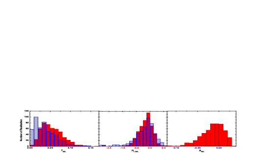
Figure 1: The distribution of $r_{\rm ML}$, $n_{t{\rm ML}}$ and $z_{\rm ML}$ for the $500$ simulated samples. The blue shadow shows the results by adopting the free parameters $r$ and $n_{t}$ and the flat prior of them. The red column shows the results by adopting the free parameters $r$ and $z$ and the flat prior of them.

III Understanding the statistical bias

It is important to understand why this statistical bias does exist. In order to realize it, let us proceed the following analytical approximation for the likelihood analysis.

The primordial power spectrum of RGW in (1) can be rewritten as,

$$P_{t}(k)=A_{t}(k_{0})\left({k}/{k_{0}}\right)^{n_{t}}=A_{s}(k_{0})r\exp\left[n_{t}\ln\left({k}/{k_{0}}\right)\right],$$ (2)

which can be approximated as

$$P_{t}(k)\simeq A_{s}(k_{0})\left[r+rn_{t}\ln\left({k}/{k_{0}}\right)\right].$$ (3)

In this approximation, we have used $|n_{t}|\ll 1$.

The total CMB power spectra $C_{\ell}^{Y}$ ($Y=T,C,E,B$) include the contributions of density perturbations and gravitational waves, i.e.

$$C_{\ell}^{Y}=C_{\ell,s}^{Y}+C_{\ell,t}^{Y},$$ (4)

where $C_{\ell,s}^{Y}$ and $C_{\ell,t}^{Y}$ are the contributions of density perturbations and gravitational waves, separately. Note that $C_{\ell,s}^{B}=0$. By considering $|n_{t}|\ll 1$, the spectra $C_{\ell,t}^{Y}$, as a function of $r$ and $n_{t}$, can be approximated as zb

$$C_{\ell,t}^{Y}\simeq\mathcal{C}_{\ell,t}^{Y}\left[r+rn_{t}\ln\left({\ell}/{\ell_{0}}\right)\right].$$ (5)

Here $\mathcal{C}_{\ell,t}^{Y}\equiv C_{\ell,t}^{Y}(r=1,n_{t}=0)$, and best-pivot multipole $\ell_{0}=k_{0}\times 10^{4}$Mpc zb . So $P_{t}(k)$ and $C_{\ell,t}^{Y}$ are all the linear combinations of the parameters $r$ and $rn_{t}$.

Now, let us turn to the likelihood function. The exact form can be found in the previous works lewis zbg ; zhao ; zb . In the analytical approximation, it can be well approximated by zb

$$-2\ln\mathcal{L}=\sum_{\ell}\sum_{Y}\left(\frac{D_{\ell}^{Y}-C_{\ell}^{Y}}{\hat{\sigma}_{D_{\ell}^{Y}}}\right)^{2}.$$ (6)

$D_{\ell}^{Y}$ is the observable data, and $\hat{\sigma}_{D_{\ell}^{Y}}$ is standard deviation of $D_{\ell}^{Y}$. The likelihood function (6) can be rewritten as zb

$$-2\ln\mathcal{L}=\sum_{\ell}\sum_{Y}\left[d_{\ell}^{Y}-(r+rn_{t}b_{\ell})a_{\ell}^{Y}\right]^{2}$$ (7)

where we have defined the quantities

$$d_{\ell}^{Y}\equiv\frac{D_{\ell}^{Y}-C_{\ell,s}^{Y}}{\hat{\sigma}_{D_{\ell}^{Y}}},~{}~{}a_{\ell}^{Y}\equiv\frac{\mathcal{C}_{\ell,t}^{Y}}{\hat{\sigma}_{D_{\ell}^{Y}}},~{}~{}b_{\ell}^{Y}\equiv\ln(\ell/\ell_{0}),$$ (8)

which are all independent of the variables $r$ and $n_{t}$. Obviously, the value of $d_{\ell}^{Y}$ depends on the data. For a larger number of different sample, the average value of $d_{\ell}^{Y}$ is $\langle d_{\ell}^{Y}\rangle=a_{\ell}^{Y}(\hat{r}+\hat{r}\hat{n}_{t}b_{\ell})$, due to the facts of $\langle D_{\ell}^{Y}\rangle=C_{\ell,s}^{Y}+{C}_{\ell,t}^{Y}(r=\hat{r},n_{t}=\hat{n}_{t})$ and ${C}_{\ell,t}^{Y}(r=\hat{r},n_{t}=\hat{n}_{t})\simeq\mathcal{C}_{\ell}^{Y}(\hat{r}+\hat{r}\hat{n}_{t}b_{\ell})$.

Since we have adopted the best-pivot multipole $\ell_{0}$, which is defined by requiring zb $\sum_{\ell}\sum_{Y}(a_{\ell}^{Y})^{2}b_{\ell}=0$, the likelihood (7) can be rewritten as zb

$$-2\ln\mathcal{L}=\left(\frac{r-r_{p}}{r_{s}}\right)^{2}+\left(\frac{rn_{t}-z_{p}}{z_{s}}\right)^{2}+C,$$ (9)

where $C$ is a constant, and the other quantities are defined by

$$r_{p}\equiv\frac{\sum_{\ell}\sum_{Y}a_{\ell}^{Y}d_{\ell}^{Y}}{\sum_{\ell}\sum_{Y}(a_{\ell}^{Y})^{2}},~{}~{}r_{s}\equiv\frac{1}{\sqrt{\sum_{\ell}\sum_{Y}(a_{\ell}^{Y})^{2}}},$$ (10)

$$z_{p}\equiv\frac{\sum_{\ell}\sum_{Y}a_{\ell}^{Y}d_{\ell}^{Y}b_{\ell}}{\sum_{\ell}\sum_{Y}(a_{\ell}^{Y}b_{\ell})^{2}},~{}~{}z_{s}\equiv\frac{1}{\sqrt{\sum_{\ell}\sum_{Y}(a_{\ell}^{Y}b_{\ell})^{2}}}.$$ (11)

The posterior pdf relates to the likelihood by the prior. Here, let us adopt the flat prior for the parameters $r$ and $n_{t}$, the 2-dimensional posterior pdf for the variables is

$$-2\ln P(r,n_{t})=\left(\frac{r-r_{p}}{r_{s}}\right)^{2}+\left(\frac{rn_{t}-z_{p}}{z_{s}}\right)^{2},$$ (12)

which follows the 1-dimensional posterior pdf for $r$ as follows,

$$P(r)=\frac{1}{r}\exp\left[-\frac{1}{2}\left(\frac{r-r_{p}}{r_{s}}\right)^{2}\right]+C^{\prime}.$$ (13)

We notice that, when $r_{p}\gg r_{s}$, corresponding to $S/N\gg 1$ (see zb for details), this pdf can be reduced that

$$P(r)\simeq\frac{1}{r_{p}}\exp\left[-\frac{1}{2}\left(\frac{r-r_{p}}{r_{s}}\right)^{2}\right]+C^{\prime}.$$ (14)

This is gaussian function for $r$, and peaks at $r=r_{p}$ with spread $r_{s}$. From the expression of $r_{p}$, we know that, the value of $r_{p}$ depends on the data $D_{\ell}^{Y}$ by the quantity $d_{\ell}^{Y}$. However, the average value of $r_{p}$ for a larger number of sample is $\bar{r}_{p}=\hat{r}$, i.e. $r_{p}$ is an unbiased estimator for $\hat{r}$. This has been mentioned in the previous paper zb .

But here, we want to emphasize that, when $r_{p}$ is not much larger than $r_{s}$, the peak of the posterior pdf in (13) is smaller than $r_{p}$, due to the term $1/r$. Especially when $r_{p}<3r_{s}$, the peak of the pdf is very close to zero, which is never an unbiased estimator for the input value $\hat{r}$. This explains what we have found in the left panel of Fig.1.

IV Avoiding the statistical bias

Now, let us consider the possible way to avoid this bias in the data analysis. Let us return to the likelihood function in (9). We find that, if considering $r$ and $z\equiv rn_{t}$ as two independent parameters, this likelihood is a simple gaussian function for the uncorrected parameters $r$ and $z$.

Now, we adopt the flat prior for the variables $r$ and $z$, and the posterior pdf for $r$ and $z$ becomes

$$-2\ln P(r,z)=\left(\frac{r-r_{p}}{r_{s}}\right)^{2}+\left(\frac{z-z_{p}}{z_{s}}\right)^{2},$$ (15)

from which follows that the 1-dimensional posterior pdf for $r$ is

$$P(r)=\exp\left[-\frac{1}{2}\left(\frac{r-r_{p}}{r_{s}}\right)^{2}\right]+C^{\prime}.$$ (16)

This pdf peaks at $r=r_{p}$, which is an unbiased estimator for the input value $\hat{r}$. Similarly, we can also find that, the 1-dimensional posterior pdf for $z$ peaks at $z=z_{p}$, which is also an unbiased estimator for $\hat{z}\equiv\hat{r}\hat{n_{t}}$. So the statistical bias in data analysis is elegantly avoided.

In order to clearly show this result, we have analyzed the same $500$ samples, by adopting the flat prior on $r$ and $z$. In Fig.1, we plot the distribution of the $r_{\rm ML}$ and $z_{\rm ML}$ with the solid columns. As expected, we find that, these $r_{\rm ML}$ and $z_{\rm ML}$ are all distributed around at their input values $\hat{r}=0.05$ and $\hat{z}=0$, and the bias for the tensor-to-scalar ratio is naturally avoided. In this figure, we also plot the distribution of $n_{t{\rm ML}}$, which also unbiased distributed around its input value $\hat{n}_{t}=0$.

It is interesting to compare the difference between the prior $f(r,z)$ and the general prior $f(r,n_{t})$. They can be related by the Jacobi, i.e.

$$f(r,n_{t})=\left|\frac{\partial(r,z)}{\partial(r,n_{t})}\right|f(r,z)=rf(r,z).$$ (17)

This relation shows that, the flat prior $f(r,z)=1$ exactly corresponds to $f(r,n_{t})=r$. So, comparing with the analysis with flat prior $f(r,n_{t})=1$, the new flat prior $f(r,z)$ induces a larger value of the variable $r$.

V conclusion

In this Letter, we find a statistical bias in the CMB data analysis for the detection of RGWs, when the signal-to-noise ratio is not very high. This could overlook the signal of RGWs in the CMB data analysis. We explain why this bias does exist by the analytical approximation of the likelihood function, and also find this bias can be elegantly avoided by adopting the orthogonalized parameters $r$ and $z\equiv rn_{t}$, instead of the general parameters $r$ and $n_{t}$.

In the end, we should emphasize that a similar statistical bias might exist for any data analysis prior , which should be carefully treated.

Acknowledgement: The author thanks D.Baskaran, L.P. Grishchuk, P.Coles, H.Chiaka, S.Gupta for helpful discussions. This work is supported by NSFC grants Nos. 10703005, 10775119 and 11075141.

References

- (1) L.P. Grishchuk, Zh. Eksp. Teor. Fiz. 67, 825 (1974); Ann. N. Y. Acad. Sci 302, 439 (1977); Pis’ma Zh. Eksp. Teor. Fiz. 23, 326 (1976); Uspekhi Fiz. Nauk 121, 629 (1977).
- (2) A. A. Starobinsky, JETP Lett. 30, 682 (1979); Phys. Lett. B 91, 99 (1980).
- (3) B. P. Abbott et al., (LIGO Scientific Collaboration and Virgo Collaboration), Nature (London) 460, 990 (2009).
- (4) S. Hild et al., arXiv:1012.0908; C. Van Den Broeck et al., private communication.
- (5) F. Jenet et al., Astrophys. J. 653, 1571 (2006).
- (6) R. van Haasteren et al., arXiv:1103.0576; W. Zhao, Phys. Rev D 83, 104021 (2011).
- (7) B. Allen and J. D. Romano, Phys. Rev. D 59, 102001 (1999).
- (8) T. L. Smith, E. Pierpaoli and M. Kamionkowski, Phys. Rev. Lett. 97, 021301 (2006).
- (9) U. Seljak and M. Zaldarriaga, Phys. Rev. Lett. 78, 2054 (1997); M. Kamionkowski, A. Kosowsky and A. Stebbins, Phys. Rev. Lett. 78, 2058 (1997).
- (10) J. R. Printchard and M. Kamionkowski, Ann. Phys. (N.Y.) 318, 2 (2005); W. Zhao and Y. Zhang, Phys. Rev. D 74, 083006 (2006); D. Baskaran, L. P. Grishchuk and A. G. Polnarev, Phys. Rev D 74, 083008 (2006).
- (11) E. Komatsu et al., Astrophys. J. Suppl. Ser. 192, 18 (2011).
- (12) W. Zhao and L. P. Grishchuk, Phys. Rev. D 82, 123008 (2010).
- (13) J. Bock, et al., astro-ph/0604101; D. Baumann et al., AIP Conf. Proc. 1141, 10 (2009); COrE Collaboration, arXiv:1102.2181.
- (14) Planck Collaboration, arXiv:astro-ph/0604069.
- (15) W. Zhao, Phys. Rev. D 79, 063003 (2009).
- (16) W. Zhao, D. Baskaran and L.P. Grishchuk, Phys. Rev. D 79, 023002 (2009), Phys. Rev. D 80, 083005 (2009).
- (17) E. Komatsu et al., Astrophys. J. Suppl. Ser. 180, 330 (2009).
- (18) W. Zhao and D. Baskaran, Phys. Rev. D 79, 083003 (2009).
- (19) S. Hamimeche and A. Lewis, Phys. Rev. D 77, 103013 (2008).
- (20) e.g. W. Valkenburg, L.M. Krauss and J. Hamann, Phys. Rev. D 78, 063521 (2008).