Luminosities of recycled radio pulsars in globular clusters

Abstract

Using Monte Carlo simulations, we model the luminosity distribution of recycled pulsars in globular clusters as the brighter, observable part of an intrinsic distribution and find that the observed luminosities can be reproduced using either log-normal or power-law distributions as the underlying luminosity function. For both distributions, a wide range of model parameters provide an acceptable match to the observed sample, with the log-normal function providing statistically better agreement in general than the power-law models. Moreover, the power-law models predict a parent population size that is a factor of between two and ten times higher than for the log-normal models. We note that the log-normal luminosity distribution found for the normal pulsar population by Faucher-Giguère and Kaspi is consistent with the observed luminosities of globular cluster pulsars. For Terzan 5, our simulations show that the sample of detectable radio pulsars, and the diffuse radio flux measurement, can be explained using the log-normal luminosity law with a parent population of $\sim 150$ pulsars. Measurements of diffuse gamma-ray fluxes for several clusters can be explained by both power-law and log-normal models, with the log-normal distributions again providing a better match in general. In contrast to previous studies, we do not find any strong evidence for a correlation between the number of pulsars inferred in globular clusters and globular cluster parameters including metallicity and stellar encounter rate.

1 Introduction

The first millisecond radio pulsar in a globular cluster (GC) was discovered by Lyne et al. (1987), shortly after earlier predictions that the putative progenitors of millisecond pulsars (MSP) are low-mass X-ray binaries (Alpar et al., 1982) which are known to be present in GCs (Katz, 1975). Inspired by this discovery, a large number of sensitive pulsar searches have been performed over the years resulting in the currently observed population of 143 radio pulsars in 27 GCs. GCs have some physical properties which are different than those of the galactic disk. Examples are extremely high stellar density and high abundance of metal poor population II stars indicating that they were born in the early phase of the Galaxy’s formation. These facts lead naturally to the question whether the population of radio pulsars in GCs is different to their counterparts in the Galactic disk. A number of differences are already well-known. In particular, the high abundance of MSPs both in eccentric binary systems and as isolated objects. These phenomena can be explained as the results of two-body or three-body stellar interactions in the dense stellar environment of GCs (Romani, Kulkarni, & Blandford, 1987; Verbunt et al., 1987; Ivanova et al., 2008; Bagchi & Ray, 2009). On the other hand, the luminosity of a pulsar is a more fundamental property as it can in principle be linked to the pulsar emission mechanism. It is therefore important to establish whether there is any evidence for a different luminosity function of MSPs in the disk compared to those in GCs.

There are two main ways to determine the pulsar luminosity function numerically: (i) a full dynamical approach; (ii) a snapshot approach. In the dynamical approach, a simulation is performed in which a model galaxy of pulsars is seeded according to various prescriptions of birth locations and initial rotational parameters. Each of these synthetic pulsars is then “evolved” both kinematically in a model for the Galactic gravitational potential and rotationally using a model for neutron star spin-down. The resulting population is then passed through the various detection criteria (see, e.g., Faucher-Giguère & Kaspi, 2006). The resulting set of “detectable” pulsars is then compared to the observed sample. The snapshot approach differs from the dynamical approach in that the pulsars are seeded at their final positions in the galaxy without assuming anything about their spin-down or kinematic evolution and thus form a picture of the present day population.

The dynamical approach has been used extensively to study normal pulsars in the galactic disk (Bhattacharya et al., 1992; Gonthier et al., 2002; Faucher-Giguère & Kaspi, 2006; Ridley & Lorimer, 2010). These studies considered the luminosity of pulsars to be described by power-law functions involving $P$ and $\dot{P}$ with a substantial dispersion to account for distance uncertainties and beam geometry. One of the conclusions by Faucher-Giguère & Kaspi (2006, hereafter FK06), also verified by Ridley & Lorimer (2010) is that the resulting parent population of luminosities appears to be well described by a log-normal function. As discussed further in Section 3.1, the log-normal parameters favored by FK06 (for the base-10 logarithm of the 1400-MHz luminosities) are a mean of –1.1 and a standard deviation of 0.9. One of the goals of the current study is to examine whether these log-normal parameters are consistent with the observed populations of GC pulsars.

For pulsars in GCs, where it is difficult to model the effects of stellar encounters and the cluster potential, the dynamical approach has so far not been used for radio pulsar population syntheses. Although such an approach may be tractable in future, we will adopt in this work a version of the snapshot approach. We will carry out Monte Carlo simulations that assume all GCs have the same intrinsic pulsar luminosity function, but a different population size and use this approach to model the observed sample of pulsars given the various ranges of luminosities. As we shall see, this approach provides a remarkably good agreement between the model and observed luminosity distributions.

Within the snapshot framework, one usually fits the complementary cumulative distribution function (CCDF) of pulsar luminosity as a power law as $N(>L_{1400})=N_{0}L_{1400}^{q}$, where $L_{1400}$ is the luminosity of the pulsar at 1400 MHz, $N$ is the number of pulsars having luminosity value greater than $L_{1400}$, $N_{0}$ and $q$ are constants. We note here that sometimes in literature (Hessels et al., 2007; Hui, Cheng & Taam, 2010), the CCDF has been mentioned as the cumulative distribution function; but actually the cumulative distribution function (CDF, $N(\leq L_{1400})$ ) is related to the CCDF as CDF = $1-$ CCDF. Using this snapshot technique, Hui, Cheng & Taam (2010) concluded that the luminosities of MSPs in GCs are different from those in the galactic disk as the CCDF for GC MSPs is much steeper than that of disk pulsars. This is a very important conclusion. If correct, it would imply that the radio luminosity is related to differences in formation processes between the disk and GC pulsars. The same analysis was re-performed with more recent distance estimates of GCs and the resultant CCDF was even steeper (Bagchi & Lorimer, 2010).

Since GCs are generally at large distances, the luminosity function of observed pulsars is not as well sampled as in the Galactic disk. In the present work we try to account for this incompleteness by considering GC MSPs as the brighter tail of some intrinsic parent population. The goal of the current work is to explore the range of possible distributions that are consistent with the current sample of GC pulsars. The plan for the rest of this paper is as follows. In Section 2, we describe the pulsar sample we use. In Section 3, we present our analysis procedure and its main results. In Section 4, we investigate additional constraints on allowed model parameters from observations of diffuse radio and gamma-ray flux. In Section 5, we compare our results with earlier work. We draw our main conclusions in Section 6.

2 The observational sample

The luminosity of a pulsar, $L$, can be computed (see, e.g., Lorimer & Kramer, 2005) from its distance and the mean flux density $S_{\nu}$ (defined at some observing frequency $\nu$) using the following geometrical relationship:

$$L=\frac{4\pi d^{2}}{\delta}\,{\rm sin^{2}}\left(\frac{\rho}{2}\right)\int_{\nu_{\rm low}}^{\nu_{\rm up}}S_{\nu}d\nu.$$ (1)

Here $\rho$ is the radius of the (assumed circular) emission cone, $\delta$ is the pulse duty cycle ($=W_{\rm eq}/P$), $P$ is the spin period of the pulsar and $W_{\rm eq}$ is the equivalent width of the pulse (i.e. the width of a top-hat shaped pulse having the same area and peak flux density as the true profile), $\nu_{\rm low}$ and $\nu_{\rm up}$ defines the range of radio frequencies over which the pulsar has been observed and $d$ is the distance of the pulsar. As it is usually difficult to determine the values of $\rho$ and $\delta$ reliably, we define the “pseudoluminosity”

$$L_{\nu}=S_{\nu}~{}d^{2}.$$ (2)

Henceforth, we will use the term luminosity to mean pseudoluminosity.

Among the current sample of 143 GC pulsars, flux density values have been reported for 107 pulsars. Among these, three are clearly young isolated objects which more closely resemble the normal population of pulsars in the Galaxy (for a further discussion of this population, see Boyles et al., 2011). We consider here the sample of 83 pulsars in 10 GCs with spin periods $P\leq 100$ ms and each of these GCs host at least 4 such pulsars. For all these objects, the spin and binary properties suggest that the neutron star has undergone a phase of recycling in the past.

Among these, for 45 pulsars (14 in 47 Tuc, 4 in M 3, 5 in M 5, 5 in M 13, 5 in NGC 6752, 3 in NGC 6517 and 9 in M 28) flux density values have been measured at 1400 MHz; for 31 pulsars (25 in Terzan 5, 5 in NGC 6440 and 1 in NGC 6517) flux density values have been measured at 1950 MHz and for 7 pulsars (in M 5) flux density values have been measured at 400 MHz. To pursue our study of pulsar luminosities at 1400 MHz, we scale the flux densities measured at other frequencies using the power-law $S_{\nu}\propto\nu^{\alpha}$, where $\alpha$ is the spectral index. We then use the model prediction for $S_{1400}$ as the best estimate of the pulsar’s flux density at this frequency. In these calculations we use the estimated values of $\alpha$ from observed values of fluxes at different frequencies whenever available, otherwise adopt the mean $\alpha$ of GC MSPs (for which flux values have been reported at multiple frequencies) of $-1.9$. Toscano et al. (1998) also obtained mean $\alpha$ of 19 millisecond pulsars to be $-1.9\pm 0.1$, but their sample contains only two GC pulsars. Once we get $S_{1400}$, we can calculate $L_{1400}$ if $d$ is known. For GC pulsars, the distances are taken to be those of their host clusters. We use the most recent distance estimates from the literature.

Table 1: Fluxes and spectral indices of 107 pulsars in globular clusters. $\alpha$ can be calculated for 20 pulsars using the central frequency of observations (when ever reported). Mean $\alpha$ of pulsars having $P_{s}\leq$ 100 ms is –1.865 (excluding positive $\alpha$ of PSR J1836$-$2354A). We set $\alpha=-1.9$ in the present work. From the sample of 107 pulsars, we exclude pulsars with spin period $>$ 100 ms; and then exclude pulsars for which the host GC contains less than 4 pulsars with $P_{s}\leq$ 100 ms and known flux values. Pulsars which are not used in the present study have been written in italics. References are at the end of the table.

GC	PSR	$P_{s}$	$S_{400}$	$S_{600}$	$S_{1170}$	$S_{1400}$	$S_{1600}$	$S_{1950}$	$\alpha$
		(ms)	(mJy)	(mJy)	(mJy)	(mJy)	(mJy)	(mJy)
47 Tuc	J0023-7204C	5.757	1.53(r1)	1.54(r1)	*	0.36(r2)	*	*	-1.352
47 Tuc	J0024-7204D	5.358	0.95(r1)	0.55(r1)	*	0.22(r2)	*	*	-1.264
47 Tuc	J0024-7205E	3.536	*	*	*	0.21(r2)	*	*	*
47 Tuc	J0024-7204F	2.624	*	*	*	0.15(r2)	*	*	*
47 Tuc	J0024-7204G	4.040	*	*	*	0.05(r2)	*	*	*
47 Tuc	J0024-7204H	3.210	*	*	*	0.09(r2)	*	*	*
47 Tuc	J0024-7204I	3.485	*	*	*	0.09(r2)	*	*	*
47 Tuc	J0023-7203J	2.101	*	*	*	0.54(r2)	*	*	*
47 Tuc	J0024-7204L	4.346	*	*	*	0.04(r2)	*	*	*
47 Tuc	J0023-7205M	3.677	*	*	*	0.07(r2)	*	*	*
47 Tuc	J0024-7204N	3.054	*	*	*	0.03(r2)	*	*	*
47 Tuc	J0024-7204O	2.643	*	*	*	0.10(r2)	*	*	*
47 Tuc	J0024-7204Q	4.033	*	*	*	0.05(r2)	*	*	*
47 Tuc	J0024-7203U	4.343	*	*	*	0.06(r2)	*	*	*
NGC 1851	J0514-4002	4.990	0.28(r3)	*	*	*	*	0.0056(r3)	-2.568
M 53	B1310+18	33.163	1.0(r4)	*	*	*	*	*	*
M 3	J1342+2822A	2.545	*	*	*	0.007(r5)	*	*	*
M 3	J1342+2822B	2.389	*	*	*	0.014(r5)	*	*	*
M 3	J1342+2822C	2.166	*	*	*	0.006(r5)	*	*	*
M 3	J1342+2822D	5.443	*	*	*	0.010(r5)	*	*	*
M 5	B1516+02A	5.554	0.5(r6)	*	0.155(r7)	0.120(r5)	*	*	-1.161
M 5	B1516+02B	7.947	0.3(r6)	*	0.027(r7)	0.025(r5)	*	*	-2.132
M 5	J1518+0204C	2.484	*	*	*	0.039(r5)	*	*	*
M 5	J1518+0204D	2.988	*	*	*	0.008(r5)	*	*	*
M 5	J1518+0204E	3.182	*	*	*	0.010(r5)	*	*	*
M 4	B1620-26	11.076	15(r8)	7.2(r9)	*	1.6(r10)	*	*	-1.744
M 13	B1639+36A	10.378	3.0(r4)	*	*	0.140(r5)	*	*	-2.486
M 13	B1639+36B	3.528	*	*	*	0.022(r5)	*	*	*
M 13	J1641+3627C	3.722	*	*	*	0.030(r5)	*	*	*
M 13	J1641+3627D	3.118	*	*	*	0.024(r5)	*	*	*
M 13	J1641+3627E	2.487	*	*	*	0.010(r5)	*	*	*
M 62	J1701-3006A	5.242	*	*	*	0.4(r11)	*	*	*
M 62	J1701-3006B	3.594	*	*	*	0.3(r11)	*	*	*
M 62	J1701-3006C	7.613	*	*	*	0.3(r11)	*	*	*
NGC 6342	B1718-19	1004.04	0.253(r12)	0.550(r12)	*	0.278(r12)	0.18(r12)	*	-0.338
NGC 6397	J1740-5340	3.650	*	*	*	1.0(r13)	*	*	*
Ter 5	J1748-2446A	11.563	*	5(r14)	*	0.61(r15)	*	1.020(r16)	-1.572
Ter 5	J1748-2446C	8.436	*	*	*	*	*	0.360(r16)	*
Ter 5	J1748-2446D	4.714	*	*	*	*	*	0.041 (r16)	*
Ter 5	J1748-2446E	2.198	*	*	*	*	*	0.048(r16)	*
Ter 5	J1748-2446F	5.540	*	*	*	*	*	0.035(r16)	*
Ter 5	J1748-2446G	21.672	*	*	*	*	*	0.015(r16)	*
Ter 5	J1748-2446H	4.926	*	*	*	*	*	0.015(r16)	*
Ter 5	J1748-2446I	9.570	*	*	*	*	*	0.029(r16)	*
Ter 5	J1748-2446J	80.338	*	*	*	*	*	0.019(r16)	*
Ter 5	J1748-2446K	2.970	*	*	*	*	*	0.040(r16)	*
Ter 5	J1748-2446L	2.245	*	*	*	*	*	0.041(r16)	*
Ter 5	J1748-2446M	3.570	*	*	*	*	*	0.033(r16)	*
Ter 5	J1748-2446N	8.667	*	*	*	*	*	0.055(r16)	*
Ter 5	J1748-2446O	1.677	*	*	*	*	*	0.120(r16)	*

Table 1: (continued).

Table 1: (continued).

References : (1) r1 : Robinson et al. (1995), (2) r2 : Camilo et al. (2000), (3) r3 : Freire, Ransom & Gupta (2007), (4) r4 : Kulkarni et al. (1991), (5) r5 : Hessels et al. (2007), (6) r6 : Anderson et al. (1997), (7) r7 : Freire et al. (2008a), (8) r8 : unpublished (http://www.atnf.csiro.au/research/pulsar/psrcat/expert.html), (9) r9 : Toscano et al. (1998), (10) r10 : Kramer et al. (1998), (11) r11 : Possenti et al. (2003), (12) r12 : Averaged over variations with the orbital phase (Lyne et al., 1993), (13) r13 : D’Amico et al. (2001), (14) r14 : Lyne et al. (1990), (15) r15 : Hobbs et al. (2004), (16) r16 : Ransom et al. (2005), (17) r17 : Hessels et al. (2006), (18) r18 : Lyne et al. (1996), (19) r19 : Freire et al. (2008b), (20) r20 : Lynch et al. (2011), (21) r21 : Lorimer et al. (1995), (22) r22 : Ransom et al. (2001), (23) r23 : Biggs et al. (1994), (24) r24 : Foster, Fairhead, & Backer (1991), (25) r25 : Bégin (2006), (26) r26 : Corongiu et al. (2006), (27) r27 : Anderson (1993), (28) r28 : Wolszczan et al. (1989), (29) r29 : Ransom et al. (2004)

Figure 1: Complementary cumulative distribution of 1400-MHz luminosities for the sample of globular cluster pulsars. Flux density values measured at other frequencies have been converted to $S_{1400}$ using $S_{\nu}\propto\nu^{\alpha}$ for $\alpha=-1.9$. We have checked that a change in the value of $\alpha\sim\pm 0.3$ does not make any visible change in the shape of the plot.

Our complete list of GC pulsar flux and spectral parameters used in this section, and the remainder of the paper is given in Table 2. While compiling this list, we confirmed the earlier conclusions by Hessels et al. (2007) that the choice of $\alpha$ in a realistic range does not affect the complementary cumulative distribution (CCD) of luminosities significantly. Using 37 isolated GC pulsars, Hessels et al. (2007) found that an arbitrary choice of $\alpha$ in the range of –1.6 to –2.0 does not affect the shape of the CCD. We arrive at the same conclusion with our sample using different values of $\alpha$ as –1.6, –1.9 and –2.2. We perform Kolmogorov-Smirnov (KS) tests between the luminosity distributions obtained with different choice of $\alpha$. The KS test returns a statistic $P_{\rm KS}$ which gives the probability that the two samples are drawn from the same distribution (for details, see Press et al. , 2007). In this case, $P_{\rm KS}$ is always greater than $0.997$ when we compare any two luminosity distributions from the three obtained with $\alpha=-1.6$, $-1.9$ and $-2.0$; as an example, the distribution obtained with $\alpha=-1.9$ is shown in Fig. 1.

The absence of any significant difference in the luminosity distribution for a realistic range of $\alpha$ also supports our choice of $\alpha=-1.9$ for this work, which is not too different than the favored choice ($\alpha=-1.8$) of other studies (Hui, Cheng & Taam, 2010; Maron, Kijak, Kramer & Wielebinski, 1987). As we are studying luminosities only at 1400 MHz, henceforth, we shall denote $L_{1400}$ simply by $L$.

Note also that, throughout this paper, we will be concerned with the possible forms of the luminosity distribution of cluster pulsars. Correlations between luminosity and other pulsar parameters are not discussed in any detail here. The reason for this is that, as for the pulsar population in the Galaxy correlations in the observed pulsar samples are not apparent due to the presence of distance errors and beaming uncertainties (see Lorimer et al. 1993 for a discussion). We did not find any correlation between luminosity and spin period of the 83 recycled pulsars used in the present work. As mentioned earlier, $\dot{P}$ measurements for globular cluster pulsars are affected by cluster potential, so can not easily be used to study intrinsic properties of the pulsars. For the remainder of this paper, we proceed with the underlying assumption that there exists a single luminosity function for all globular cluster pulsars, and attempt to explain the observed luminosities in this way. As we will demonstrate, the data are remarkably consistent with this simple idea. However, the wide ranges of possible model parameters that are consistent with the data do not rule out the idea that the parent luminosity function may vary from cluster to cluster.

3 Analysis

With the data described above, we aim to find luminosity distribution functions whose brighter tail can be considered as the observed luminosity distribution of GC pulsars, assuming that the parent luminosity distribution is the same for all GCs. To do so, for each GC, we first generate a synthetic sample of $N_{\rm trial,i}$ pulsar luminosities from a chosen distribution function until we get $C\times N_{\rm obs,i}$ pulsars having simulated luminosities greater than the observed minimum luminosity for that GC. This multiplication by the constant ‘$C$’ (100–1000) is done to minimize statistical variations. In this notation, $i$ is the GC index $N_{\rm obs,i}$ is the observed number of pulsars in the GC that we consider,

$$L_{\rm sim,tot}=\frac{1}{C}\displaystyle\sum\limits_{j=1}^{N_{\rm trial,i}}L_{\rm sim,j}$$ (3)

is the total luminosity and

$$S_{\rm sim,tot}=\frac{1}{C}\displaystyle\sum\limits_{j=1}^{N_{\rm trial,i}}S_{\rm sim,j}$$ (4)

is the total flux in the $i^{\rm th}$ GC. Here $L_{\rm sim,j}$ and $S_{\rm sim,j}$ are the simulated luminosities and corresponding fluxes. After we perform the simulation for all 10 GCs, we compare the simulated luminosities with the observed luminosities of 83 pusars by performing KS and $\chi^{2}$ tests. As mentioned earlier, the KS test can be used to test the hypothesis that two distributions differ, with a low value of KS probability $P_{\rm KS}$ suggesting a mismatch. The $\chi^{2}$ statistic uses binned data and compares the values of the two distributions at each bin; here a low value of $\chi^{2}$ implies a good agreement. Here we divide the luminosity range 0.1–1000 ${\rm mJy~{}kpc^{2}}$ into 36 logarithmically equispaced bins. $N_{\rm trial,i}/C$ is the predicted number of total pulsars in that GC which we call as $N_{\rm rad,i}$.

A key assumption in our present analysis is that each GC has been searched down to the level of the faintest observable pulsar in that particular cluster. This assumption provides a good approximation to the actual survey sensitivity in each cluster, and was made primarily due to the lack of currently published detail of several of the globular cluster surveys so far. The assumption greatly simplifies our modeling procedure, since it means that we do not have to consider variations in sensitivity due to other factors (for example scintillation, eclipsing binary systems etc.). This simple approach is appropriate for the purposes of the current work where we are simply trying to assess the range of luminosity functions compatible with the data. A more rigorous study which takes account of the survey thresholds in detail may well be able to narrow the range of possible model parameters found here, and should certainly be carried out when more details of the surveys are published, but is beyond the scope of the current work.

3.1 Log-normal luminosity function

We begin by testing a log-normal luminosity function, where the probability density function (PDF)

$$f_{\rm log-normal}\,(L)=\frac{\log_{10}e}{L}\,\frac{1}{\sqrt{2\pi\sigma^{2}}}\,\exp\left[{\frac{-(\log_{10}L-\mu)^{2}}{2\sigma^{2}}}\right],$$ (5)

where, as usual, $\mu$ is the mean of the distribution and $\sigma$ is the standard deviation. For this choice of distribution, we find that $C=100$ is sufficient to minimize statistical fluctuations. The variation of $P_{\rm KS}$ and $\chi^{2}$ with $\mu$ and $\sigma$ are shown in Fig. 2. It is clear that there is a wide range of values of $\mu$, $\sigma$ for which the simulated luminosity distributions agree well with the observed sample. For the two statistical tests, good agreement is given when $P_{\rm KS}$ has high values and $\chi^{2}$ is small. As expected, the region of $\mu-\sigma$ parameter space encompassed by $P_{\rm KS}>0.05$ is essentially the same as the contours encompassing the 95% probability values around the $\chi^{2}$ minimum.

For this distribution, and for the purposes of later discussion, we define three models based on particular parameter choices. Model 1 uses the parameters found by FK06 ($\mu=-1.1$ and $\sigma=0.9$) from which we find $P_{\rm KS}=0.15$ and $\chi^{2}=9.4$. Model 2, for which $\mu=-0.61$ and $\sigma=0.65$ returns the maximum value of $P_{\rm KS}=0.98$ with a $\chi^{2}=7.9$. Model 3, for which $\mu=-0.52$ and $\sigma=0.62$, returns a minimum value of $\chi^{2}=6.3$ and has $P_{\rm KS}=0.37$.

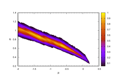
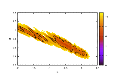
Figure 2: Top: variation of $P_{\rm KS}$ (for $P_{\rm KS}\geq 0.05$) with $\mu$ and $\sigma$. Bottom: variation of $\chi^{2}$ (within $2\sigma$ about the minimum value of $\chi^{2}$) with $\mu$ and $\sigma$, the parameters of the log-normal distribution. A $1\sigma$ contour is also shown.

Figure 3: Observed luminosity distribution with simulated luminosity distributions generated with log-normal distribution function for three different sets of $\mu$ and $\sigma$ which are defined as models 1 (upper curve), 2 (lower curve) and 3 (middle curve); see text for details. “$\ast$”s represent the observed distribution.

In Fig. 3 we compare these three models with the observed data. As expected, all models match well. While model 3 provides the closest match by eye, the statistical results mentioned above do not rule out either model 1 or model 2. The FK06 luminosity model parameters (model 1), therefore, are consistent with the observed CCD.

3.2 Power-law luminosity function

As mentioned earlier, power-law luminosity functions have been used by a number of authors. It is therefore of great interest to see how the power-law compares to log-normal for the GC pulsars. The PDF of the power law distribution

$$f_{\rm power-law}\,(L)=\frac{\beta L_{\rm min}^{\beta}}{L^{\beta+1}},$$ (6)

where $L_{\rm min}$ is the minimum value of $L$ and $\beta$ the power-law index. This abrupt cut-off required to avoid divergence when integrating this function over all $L$ is somewhat unphysical, but nevertheless can be used to parameterize the luminosities in an independent way to the log-normal. We perform simulations over a range of $L_{\rm min}$ 0.003—0.48 ${\rm mJy~{}kpc^{2}}$, as 0.48 ${\rm mJy~{}kpc^{2}}$ is the observed minimum luminosity among GC pulsars in our sample, and the lower value of $L_{\rm min}$ is chosen somewhat arbitrarily. For this model, we found that $C=1000$ is required to minimize statistical fluctuations. Unlike the log-normal model, we found that the power law distribution occasionally produced pulsars with large luminosities $L\gg 100$ mJy kpc² which biased some of our preliminary simulation runs. To avoid this difficulty, we imposed a maximum luminosity of 50 mJy kpc². No GC pulsar is currently known with $L>20$ mJy kpc², and our results are insensitive to the exact choice of the maximum luminosity cutoff over the range 20–500 mJy kpc².

Figure 4: Observed luminosity distribution with simulated luminosity distributions generated with a power-law distribution function for three different set of $L_{\rm min}$ and $\beta$ which are defined as models 4 (middle curve), 5 (lower curve) and 6 (upper curve); see text for details. “$\ast$”s represent the observed distribution. The mismatch between the simulated and observed CCDs appear only when the number of pulsars are $\lesssim 10$.

The nominal best parameter values give $P_{\rm KS}=0.81$ ($\chi^{2}=8.7$) for $\beta=0.92$, $L_{\rm min}=0.017{\rm~{}mJy~{}kpc^{2}}$ (model 4) and minimum $\chi^{2}=8.0$ ($P_{\rm KS}=0.56$) for $\beta=1.01$, $L_{\rm min}=0.022{\rm~{}mJy~{}kpc^{2}}$ (model 5). Our values of $\beta$ (which give good fits) are not too different from the conventional values $\beta+1=2$. For example, the best fit value of the analysis of Fruchter & Goss (2000) for Terzan 5 pulsars was $\beta+1=1.85$. We have seen that for $\beta\sim 1$, the fit does not depend much on $L_{\rm min}$ which again agrees with the results of Fruchter & Goss (2000). As an additional point of reference, we also consider the nominal power-law parameters discussed by Fruchter & Goss (2000), i.e. $\beta=0.85$ and $L_{\rm min}=0.03{\rm~{}mJy~{}kpc^{2}}$ which we refer to as model 6. For this pairing, $P_{\rm KS}=0.43$ and $\chi^{2}=9.0$. We need to remember here Fruchter & Goss (2000) did not put any constraint on the maximum value of the luminosity. In Fig. 4 we compare the observed CCD with simulated CCDs for models 4-6. Statistically, the agreement between simulated and observed distributions is almost as good as that for log-normal distributions.

3.3 Exponential Distribution

The above models characterized the luminosity function in terms of two parameters. For completeness, we also consider a simple one-parameter model, the exponential distribution with PDF

$$f_{\rm exponential}\,(L_{1400})=\lambda e^{-\lambda L}.$$ (7)

Here $1/{\lambda}$ is the mean of the distribution, and we find that $C=100$ is enough to get rid of statistical fluctuations. For this model, the maximum value of $P_{\rm KS}=0.17$ is obtained for $\lambda=0.676{\rm~{}mJy^{-1}~{}kpc^{-2}}$ with a corresponding $\chi^{2}=13.7$. The minimum value of $\chi^{2}=11.94$ is found for $\lambda=0.439{\rm~{}mJy^{-1}~{}kpc^{-2}}$ with a $P_{\rm KS}=0.00028$. In Fig. 5 we compare the observed CCD with the simulated CCDs with these two values of $\lambda$. It is clear that the simulated distribution never matches with the observed one very well. We therefore do not consider the exponential distribution further in this work and focus the remainder of the discussion on the log-normal and power-law distributions.

Figure 5: Observed luminosity distribution with simulated luminosity distributions generated with exponential distribution function with $\lambda=0.676{\rm~{}mJy^{-1}~{}kpc^{-2}}$ (lower curve) and $\lambda=0.439{\rm~{}mJy^{-1}~{}kpc^{-2}}$ (upper curve). “$\ast$”s represent the observed distribution.

4 Model predictions and constraints

In the previous section, we found that there is a large family of possible luminosity parameters that are consistent with the observed distribution of GC pulsar luminosities. These ranges translate to a variety of different predictions for the population sizes in each GC. This can be seen from a comparison of the predicted parameters for each GC using the log-normal parameter choices (models 1, 2 and 3) in Table 2 and the power-law parameter combinations (models 4, 5 and 6) in Table 3. In this section, we try to place further constraints on these parameters by examining the predictions for the diffuse radio and gamma-ray fluxes separately.

Table 2: Population estimations and predictions using log-normal luminosity functions. For each cluster, we list the predicted number of potentially observable radio pulsars ($N_{\rm rad}$), the predicted total diffuse radio flux ($S_{\rm sim,tot}$), the predicted gamma-ray luminosity ($L_{\rm\gamma,sim}$) for three different choices of efficiency ($\eta_{\gamma}$). See text for further details. To compute uncertainties in $N_{\rm rad}$, we assume that they are dominated by the statistical noise in the observed number of pulsars, $N_{\rm obs}$. The uncertainty in $N_{\rm rad}$ is then simply $N_{\rm rad}/\sqrt{N_{\rm obs}}$. Also listed for each model is $N_{10}$, the total population estimate for these 10 GCs.

Cluster	$N_{\rm rad}$	$S_{\rm sim,tot}$	$L_{\rm\gamma,sim}$
			$\langle\eta_{\gamma}\rangle=0.08$	$\langle\eta_{\gamma}\rangle=0.06$	$\langle\eta_{\gamma}\rangle=0.1$
		(mJy)	($10^{34}~{}{\rm erg~{}s^{-1}}$)
	Model 1 (FK06): $\mu=-1.1$ and $\sigma=0.9$    $N_{10}=688\pm 82$
47 Tuc	$71\pm 19$	$3.1\pm 0.8$	$10\pm 5$	$7.7\pm 3.6$	$13\pm 6$
M 3	$24\pm 12$	$0.16\pm 0.08$	$3.5\pm 2.2$	$2.6\pm 1.6$	$4.3\pm 2.7$
M 5	$24\pm 11$	$0.31\pm 0.14$	$3.5\pm 2.1$	$2.6\pm 1.6$	$4.3\pm 2.6$
M 13	$25\pm 11$	$0.38\pm 0.16$	$3.6\pm 2.1$	$2.7\pm 1.6$	$4.5\pm 2.6$
Ter 5	$167\pm 33$	$3.7\pm 0.7$	$24\pm 11$	$18\pm 8$	$30\pm 13$
NGC 6440	$88\pm 39$	$0.86\pm 0.4$	$13\pm 8$	$10\pm 6$	$16\pm 9$
NGC 6517	$46\pm 23$	$0.29\pm 0.15$	$6.6\pm 4.2$	$5.0\pm 3.1$	$8.3\pm 5.2$
M 28	$120\pm 40$	$2.6\pm 0.9$	$17\pm 9$	$13\pm 7$	$22\pm 11$
NGC 6752	$44\pm 20$	$1.7\pm 0.8$	$6.3\pm 3.8$	$4.8\pm 2.8$	$7.9\pm 4.7$
M 15	$79\pm 30$	$0.52\pm 0.20$	$11\pm 6$	$8.5\pm 4.6$	$14\pm 8$
	Model 2 (maximum $P_{ks}$): $\mu=-0.61$ and $\sigma=0.65$    $N_{10}=453\pm 56$
47 Tuc	$44\pm 12$	$2.2\pm 0.6$	$6.3\pm 3.0$	$4.8\pm 2.2$	$7.9\pm 3.8$
M 3	$15\pm 8$	$0.11\pm 0.06$	$2.2\pm 1.4$	$1.6\pm 1.1$	$2.7\pm 1.8$
M 5	$15\pm 7$	$0.20\pm 0.09$	$2.2\pm 1.3$	$1.6\pm 1.0$	$2.7\pm 1.6$
M 13	$16\pm 7$	$0.24\pm 0.11$	$2.3\pm 1.3$	$1.7\pm 1.0$	$2.9\pm 1.7$
Ter 5	$100\pm 20$	$2.6\pm 0.5$	$14\pm 6$	$11\pm 5$	$18\pm 8$
NGC 6440	$68\pm 30$	$0.75\pm 0.33$	$9.8\pm 5.8$	$7.3\pm 4.3$	$12\pm 7$
NGC 6517	$30\pm 15$	$0.21\pm 0.10$	$4.3\pm 2.7$	$3.2\pm 2.1$	$5.4\pm 3.4$
M 28	$85\pm 28$	$2.0\pm 0.7$	$12\pm 6$	$9.2\pm 4.7$	$15.3\pm 7.8$
NGC 6752	$27\pm 12$	$1.1\pm 0.5$	$3.9\pm 2.3$	$2.9\pm 1.7$	$4.9\pm 2.9$
M 15	$53\pm 20$	$0.40\pm 0.15$	$7.6\pm 4.1$	$5.7\pm 3.1$	$9.5\pm 5.2$
	Model 3 (minimum $\chi^{2}$): $\mu=-0.52$ and $\sigma=0.68$ $N_{10}=354\pm 43$
47 Tuc	$37\pm 10$	$2.5\pm 0.7$	$5.3\pm 2.5$	$4.0\pm 1.9$	$6.6\pm 3.1$
M 3	$12\pm 6$	$0.13\pm 0.06$	$1.7\pm 1.1$	$1.3\pm 0.8$	$2.2\pm 1.4$
M 5	$13\pm 6$	$0.24\pm 0.11$	$1.9\pm 1.1$	$1.4\pm 0.8$	$2.3\pm 1.4$
M 13	$14\pm 6$	$0.30\pm 0.13$	$2.0\pm 1.2$	$1.5\pm 0.9$	$2.5\pm 1.4$
Ter 5	$82\pm 16$	$2.9\pm 0.6$	$12\pm 5$	$8.9\pm 3.8$	$15\pm 6$
NGC 6440	$48\pm 21$	$0.74\pm 0.33$	$6.9\pm 4.0$	$5.2\pm 3.0$	$8.6\pm 5.1$
NGC 6517	$23\pm 12$	$0.21\pm 0.11$	$3.3\pm 2.1$	$2.5\pm 1.6$	$4.1\pm 2.7$
M 28	$63\pm 21$	$1.5\pm 0.5$	$9.1\pm 4.6$	$6.8\pm 3.5$	$11\pm 6$
NGC 6752	$21\pm 10$	$1.2\pm 0.5$	$3.0\pm 1.8$	$2.3\pm 1.4$	$3.8\pm 2.3$
M 15	$41\pm 15$	$0.43\pm 0.16$	$5.9\pm 3.2$	$4.4\pm 2.4$	$7.4\pm 3.9$

Table 3: Population estimations and predictions using power-law luminosity functions. See Table 2 for details about tabulated parameters.

Cluster	$N_{\rm rad}$	$S_{\rm sim,tot}$	$L_{\rm\gamma,sim}$
			$\langle\eta_{\gamma}\rangle=0.08$	$\langle\eta_{\gamma}\rangle=0.06$	$\langle\eta_{\gamma}\rangle=0.1$
		(mJy)	($10^{34}~{}{\rm erg~{}s^{-1}}$)
	Model 4: $L_{\rm min}=0.017$ and $\beta=0.92$ $N_{10}=3399\pm 421$
47 Tuc	$313\pm 84$	$3.4\pm 0.89$	$45\pm 21$	$34\pm 16$	$56\pm 27$
M 3	$114\pm 57$	$0.19\pm 0.09$	$16\pm 10$	$12\pm 8$	$21\pm 13$
M 5	$112\pm 50$	$0.32\pm 0.14$	$16\pm 10$	$12\pm 7$	$21\pm 12$
M 13	$118\pm 52$	$0.40\pm 0.18$	$17\pm 10$	$13\pm 8$	$21\pm 13$
Ter 5	$764\pm 153$	$4.4\pm 0.9$	$110\pm 48$	$83\pm 36$	$138\pm 60$
NGC 6440	$485\pm 217$	$1.2\pm 0.5$	$70\pm 41$	$53\pm 31$	$87\pm 52$
NGC 6517	$238\pm 119$	$0.35\pm 0.18$	$34\pm 22$	$26\pm 16$	$43\pm 27$
M 28	$628\pm 209$	$2.5\pm 0.8$	$90\pm 46$	$68\pm 35$	$113\pm 58$
NGC 6752	$216\pm 97$	$1.9\pm 0.9$	$31\pm 19$	$23\pm 14$	$39\pm 23$
M 15	$411\pm 155$	$0.68\pm 0.25$	$59\pm 32$	$449\pm 24$	$74\pm 40$
	Model 5: $L_{\rm min}=0.022$ and $\beta=1.01$ $N_{10}=3767\pm 478$
47 Tuc	$324\pm 87$	$3.3\pm 0.9$	$47\pm 22$	$35\pm 17$	$58\pm 28$
M 3	$121\pm 61$	$0.19\pm 0.09$	$17\pm 11$	$13\pm 8$	$22\pm 14$
M 5	$116\pm 52$	$0.31\pm 0.14$	$17\pm 10$	$13\pm 7$	$21\pm 12$
M 13	$123\pm 55$	$0.39\pm 0.18$	$18\pm 11$	$13\pm 8$	$22\pm 13$
Ter 5	$815\pm 163$	$4.5\pm 0.9$	$117\pm 51$	$88\pm 39$	$147\pm 64$
NGC 6440	$580\pm 260$	$1.3\pm 0.6$	$84\pm 50$	$63\pm 37$	$104\pm 62$
NGC 6517	$271\pm 136$	$0.38\pm 0.20$	$39\pm 25$	$29\pm 19$	$49\pm 31$
M 28	$714\pm 238$	$2.7\pm 0.9$	$103\pm 53$	$77\pm 30$	$129\pm 66$
NGC 6752	$237\pm 106$	$2.0\pm 0.9$	$34\pm 20$	$26\pm 15$	$43\pm 25$
M 15	$466\pm 176$	$0.73\pm 0.27$	$67\pm 36$	$50\pm 27$	$84\pm 46$
	Model 6 (FG00): $L_{\rm min}=0.03$ and $\beta=0.85$ $N_{10}=1590\pm 194$
47 Tuc	$153\pm 41$	$3.2\pm 0.86$	$22\pm 10$	$17\pm 8$	$28\pm 13$
M 3	$55\pm 28$	$0.18\pm 0.09$	$7.9\pm 5.1$	$5.9\pm 3.8$	$9.9\pm 6.3$
M 5	$54\pm 24$	$0.31\pm 0.14$	$7.8\pm 4.6$	$5.8\pm 3.4$	$9.7\pm 5.7$
M 13	$57\pm 26$	$0.38\pm 0.17$	$8.2\pm 4.9$	$6.2\pm 3.7$	$10\pm 6$
Ter 5	$363\pm 73$	$4.2\pm 0.8$	$52\pm 23$	$39\pm 17$	$65\pm 29$
NGC 6440	$216\pm 96$	$1.0\pm 0.5$	$31\pm 18$	$23\pm 14$	$39\pm 23$
NGC 6517	$112\pm 56$	$0.33\pm 0.16$	$16\pm 10$	$12\pm 8$	$21\pm 13$
M 28	$287\pm 95$	$2.2\pm 0.7$	$41\pm 21$	$31\pm 16$	$52\pm 26$
NGC 6752	$101\pm 45$	$1.8\pm 0.8$	$15\pm 9$	$11\pm 6$	$18\pm 11$
M 15	$192\pm 73$	$0.62\pm 0.23$	$28\pm 15$	$21\pm 11$	$35\pm 19$

Table 4: Observed and inferred properties of globular clusters containing pulsars used in the present work. From left to right, we list the GC name, distance from the Sun $d$ and from the Galactic center $d_{\rm gcen}$ (both in kpc), concentration parameter $c$ (base 10 logarithm of the ratio of the tidal radius to core radius), core radius $r_{c}$ (pc), base-10 logarithm of the central density ($\rho_{c}$ in solar luminosities per cubic parsec), velocity dispersion $v_{c}$ (km s^-1), base-10 logarithms of the cluster mass ($M_{GC}$ in solar masses) and base-10 logarithms of the core relaxation timescale ($t(r_{c})$ in yr), metallicity [Fe/H], normalized two body encounter rate $\Gamma_{\rm norm}$, gamma-ray flux $L_{\gamma}$ ($10^{34}$ erg s^-1) and inferred number of gamma-ray pulsars $N_{\gamma}$ from Abdo et al (2010) and Tam et al. (2011). For $\Gamma_{\rm norm}$, we first calculate the two body encounter rate for each GC as $\Gamma=\rho_{c}^{1.5}\,r_{c}^{2}$. The values of core radius have been calculated as $r_{c}=d\,{\rm tan}\,\theta_{c}$ where $\theta_{c}$ are the angular radii as quoted in the latest version of the Harris catalog (Harris, 1996, updated in December 2010). The central cluster density $\rho_{c}$, has been calculated as $\rho_{c}=\Sigma_{c}/(r_{c}\,p)$ using the values of central surface brightness $\mu_{Vc}$ (in V magnitude per square arcsecond) and the extinction coefficient $A_{V}=3.1\,E(B-V)$ where $E(B-V)$ is the color excess. $\Sigma_{c}$, the central surface brightness in $L_{V\odot}\,{\rm pc^{2}}$ can be calculated as $\log(\Sigma_{c})=0.4\,[26.392-(\mu_{Vc}-A_{V})]$ and $p$ is a parameter defined as $\log(p)=-0.603\times 10^{-c}+0.302$ (Djorgovski, 1993). Finally we normalized $\Gamma$ to $\Gamma_{\rm norm}$ considering $\Gamma=100$ for M62 (following Abdo et al, 2010). The tabulated values for $v_{c}$ and $\log(M_{\rm GC})$ can be found at http://www.astro.lsa.umich.edu/$\sim$ognedin/gc/vesc.dat (Gnedin et al., 2002).

GC	$d$	$d_{\rm gcen}$	$c$	$r_{c}$	$\log(\rho_{c})$	$v_{c}$	$\log(M_{\rm GC})$	$\log(t(r_{c}))$	[Fe/H]	$\Gamma_{\rm norm}$	$L_{\gamma}$	$N_{\gamma}$
47 Tuc	4.03	7.4	2.07	0.42	4.93	16.4	6.17	7.84	–0.72	41.27	$4.8^{+1.1}_{-1.1}$	$33^{+15}_{-15}$
M 3	10.23	12.0	1.89	1.10	3.58	9.2	5.98	8.31	–1.50	2.61	—	—
M 5	7.76	6.2	1.73	0.99	3.87	11.8	5.93	8.28	–1.29	5.83	—	—
M 13	7.13	8.4	1.53	1.28	3.55	10.3	5.89	8.51	–1.53	3.26	—	—
Ter 5	5.50	1.2	1.62	0.25	5.26	12.7	5.57	7.57	–0.23	46.50	$25.7^{+9.4}_{-8.8}$	$180^{+100}_{-90}$
NGC 6440	8.47	1.3	1.62	0.34	5.23	21.6	5.91	7.60	–0.36	78.27	$19.0^{+13.1}_{-5.0}$	$130^{+100}_{-60}$
NGC 6517	10.60	4.2	1.82	0.19	5.30	20.6	5.72	6.92	–1.23	29.71	—	—
M 28	5.70	2.7	1.67	0.40	4.86	16.3	5.74	7.62	–1.32	28.19	$6.2^{+2.6}_{-1.8}$	$43^{+24}_{-21}$
NGC 6752	4.42	5.2	2.50	0.22	5.01	7.1	5.50	6.88	–1.54	14.72	$1.4^{+0.7}_{-0.7}$	$10^{+15}_{-6}$
M 15	10.30	10.4	2.29	0.42	5.08	13.4	6.08	7.84	–2.37	66.81	$<5.8$	$<56$

4.1 Diffuse radio emission

A potentially very useful additional constraint comes from observations of the diffuse radio emission in GCs. Assuming that the only contribution to this flux is from the pulsars, then such measurements constrain the integrated luminosity function in a given cluster. Our Monte Carlo models make specific predictions for these observations (see Eqn. 4). For Terzan 5, the total radio flux $S_{\rm obs,tot}=5.2~{}{\rm mJy~{}kpc^{2}}$ (sum of diffuse flux and the fluxes of point sources) found by Fruchter & Goss (2000). Fruchter & Goss (2000) observed some other clusters too, among which NGC 6440 belongs to our list (Table 4). But as they mentioned that their observation in this cluster is consistent with the position of a single pulsar PSR B1745$-$20, we can not use this datum for our study. For 47 Tuc, McConnell et al (2004) found that $S_{\rm obs,tot}=2.0\pm 0.3~{}{\rm mJy~{}kpc^{2}}$.

Assuming both the diffuse flux measurements for Terzan 5 and 47 Tuc are dominated by their respective pulsar populations, we can confront them with the predictions from our simulations. An inspection of Tables 2 and 3 shows that the observed diffuse flux for 47 Tuc is successfully reproduced by all of the models, within the nominal uncertainties. For Terzan 5, the power law models provide a better match to the diffuse flux overall, while the log-normal models predict a slightly smaller flux that lies 2–5$\sigma$ below the nominal value found by Fruchter & Goss (2000).

Figure 6: Variations of total radio flux (upper panel) and predicted number of pulsars (lower panel) in Terzan 5 as obtained from our simulations with log-normal distribution keeping $\mu$ fixed at $-1.1$ and varying $\sigma$. The dashed lines in the upper panel denote the ranges of $S_{\rm sim,tot}=S_{\rm obs,tot}\pm 25\%$.

In Fig. 6, we fix $\mu$ to the nominal value from model 1, i.e. as found by FK06 for normal pulsars (–1.1) and vary $\sigma$. For this case, we see that there are only two possible ranges of $\sigma$ which are compatible with the diffuse flux measurement of Terzan 5: $\sigma\sim 0.5$ or $\sigma\sim 0.9$ (see the upper panel of Fig. 6). The “solution” with $\sigma\sim 0.5$, however lies well outside the $\chi^{2}$ contours shown in Fig. 2. We therefore favor the region with $\mu\sim-1.1$ and $\sigma\sim 0.9$ (the nominal FK06 values) which is consistent with both constraints. In this case, the implied total number of pulsars $N_{\rm tot}\sim 150$ (see the lower panel of Fig. 6). Further constraints on these parameters using a more detailed Bayesian analysis of these constraints for Terzan 5 will be the subject of a subsequent paper (Chennamangalam et al. in preparation).

Fig. 7 shows the analogous diagram to Fig. 6 for the power-law luminosity function for the choice $\beta=1$. In this case, there is a wide range of $L_{\rm min}$ values that are consistent with the diffuse flux measurements (upper panel of Fig. 7), and no significant additional constraints on $L_{\rm min}$ can be made. The upper bound of $S_{\rm tot}$ gives an extremely high value of $N_{\rm tot}\sim 1000$ which seems unrealistic, but the lower bound of $S_{\rm tot}$ gives $N_{\rm tot}=340$ for $L_{\rm min}=0.05~{}{\rm mJy~{}kpc^{2}}$ (lower panel of Fig. 7).

Figure 7: Variations of total radio flux (upper panel) and predicted number of pulsars (lower panel) in Terzan 5 as obtained from our simulations with Power law distribution keeping $\beta$ fixed at $1.0$ and varying $L_{\rm min}$. The dashed lines in the upper panel denote the ranges of $S_{\rm sim,tot}=S_{\rm obs,tot}\pm 25\%$.

4.2 Predicted population sizes and diffuse fluxes for different GCs

The detection of diffuse gamma-ray emission from GCs has allowed some constraints to be placed on $N_{\gamma}$, the number of gamma-ray emitting pulsars in each cluster. Following Abdo et al (2010), we can write the total gamma-ray luminosity

$$L_{\gamma}=N_{\gamma}\langle\dot{E}\rangle\,\langle\eta_{\gamma}\rangle,$$ (8)

where $\langle\dot{E}\rangle$ is the average spin-down power of MSPs, $\langle\eta_{\gamma}\rangle$ is the average spin-down to gamma-ray luminosity conversion efficiency. As the values of $\langle\dot{E}\rangle$ and $\langle n_{\gamma}\rangle$ are not well known, Abdo et al (2010) assumed $\langle\dot{E}\rangle=(1.8\pm 0.7)\times 10^{34}~{}{\rm erg~{}s^{-1}}$ and $\langle\eta_{\gamma}\rangle=0.08$. We use the values of $N_{\gamma}$ estimated using the above relationship for the clusters with gamma-ray flux (and hence luminosity) measurements.

Figure 8: Comparison of predicted number of pulsars from our simulations with those obtained from $\gamma$-ray fluxes. Top: log-normal luminosity function (FK06 parameters). Bottom: power-law luminosity function (Model 5).

In Fig. 8, we compare the estimates of $N_{\gamma}$ with our predicted numbers of radio pulsars ($N_{\rm rad}$) for one model of each luminosity function. A reasonable agreement can be noted for the log-normal function, but for the power-law function, the values of $N_{\rm rad}$ are significantly larger than those of $N_{\gamma}$. This fact remains unchanged even if we choose other models from these luminosity functions (see Tables 2 and 3). Although this simple analysis does provide some support to the log-normal models, due to the assumptions made in equation (8) and implicitly assuming that $N_{\gamma}=N_{\rm rad}$, it does not help to constrain their values significantly.

By assuming $N_{\gamma}=N_{\rm rad}$, we obtain $L_{\gamma,{\rm sim}}$ from equation (8). We tabulate $L_{\gamma,{\rm sim}}$ for different choices of $\langle\eta_{\gamma}\rangle$ for different models in Tables 2 and 3. These values can be compared with observed values of $L_{\gamma}$ and $N_{\gamma}$ as shown in Table 4. It is apparent that the $\gamma$-ray luminosities predicted by the power-law models are generally higher than observed. We note, however, that in addition to the explicit assumptions about beaming geometry mentioned above, it has been recently shown that the $\gamma$-ray observations can be biased by one or more very bright pulsars in the cluster (Freire et al., 2011), and may not be representative of the diffuse flux of the whole population.

5 Comparison with earlier results

In Fig. 9, we compare our predicted number of pulsars having $L>0.5~{}{\rm mJy~{}kpc^{2}}$ in different GCs using FK06 parameters to those by HCT10. For Terzan 5, we do not use the distance they adopted for this cluster (10.3 kpc). Instead, here we re-calculate the value of $N(L>0.5)$ by adopting exactly the same method as HCT10 using the recent estimate 5.5 kpc (Ortolani et al, 2007) to calculate luminosities. The overall agreement is good which again highlights the fact that, at least above 0.5 mJy kpc², the exact form of the luminosity function for GC pulsars is not uniquely specified by the current sample of luminosities.

Figure 9: Comparison of our predicted number of pulsars in different GCs using FK06 parameters to those by HCT10.

HCT10 used their power-law luminosity functions to search for correlations between the number of inferred radio pulsars and fundamental cluster parameters. In their Fig. 3, they present evidence for a correlation between $N_{\rm rad}$ and both cluster metallicity $[$Fe/H$]$ as well as the two-body encounter rate $\Gamma_{\rm norm}$. An inspection of these diagrams suggests that the claimed correlations are strongly influenced by Terzan 5. Adopting, for the purposes of this discussion, the parameters of model 1 (i.e. the log-normal luminosity parameters found by FK06), together with the revised distance to Terzan 5, we revisit these proposed correlations in Fig. 10. Also shown here are the results of correlation tests between $N_{\rm rad}$ and other cluster parameters. We searched for relationships between the distance of each GC and the galactic center, $d_{\rm gcen}$, the logarithm of the central luminosity density, $\rho_{c}$, the concentration parameter, $c$, the logarithm of the core relaxation time $t(r_{c})$, the cluster mass, $M_{\rm GC}$, the central velocity dispersion, $v_{c}$, and the core radius, $r_{c}$. The parameter values used for this analysis are given in Table 4.

As can be seen in Fig. 10, none of the scatter diagrams provides compelling evidence for a direct relationship between $N_{\rm rad}$ and any cluster parameters. The lack of any statistically significant correlations can also be seen formally in Table 5, where we have calculated Pearson’s correlation coefficient ($rp$) and probability at which the null hypothesis of zero correlation is disproved ($P_{rp}$), Spearman correlation coefficient ($rs$) and probability at which the null hypothesis of zero correlation is disproved ($P_{rs}$), Kendall’s $\tau$ and the probability at which the null hypothesis of zero correlation is disproved ($P_{\tau}$).

We have shown the results of correlation analyses only for FK06 (our model 1), but for other models the results are almost the same. Because both Spearman correlation and Kendall’s $\tau$ test are based on ranks, and in all the models, the GCs with descending order of ranks (based on $N_{\rm rad}$) are as follows Terzan 5, M 28, NGC 6440, M 15, 47 Tuc, NGC  6517, NGC 6752, M 13, M 3 and M 5 (with the exception in model 1 and 2 where there is a tie between M 3 and M 5, but the order of other GCs are the same, see tables 2 and 3). Even for the parametric test - Pearson’s correlation analysis, $r_{p}$ lies always within $12\%$ of that of model 1 for Fe/H and within $14\%$ of that of model 1 for $\Gamma_{\rm norm}$. This also explains why our result contradicts with that of HCT10 inspite of overall good agreement between predicted number – according to HCT10, the GCs with descending order of ranks are as follows Terzan 5, 47 Tuc, M 28, NGC 6440, NGC 6441, NGC 6752, M 13, M 5, M 3, which is different from what we obtain.

Table 5: Results of different statistical correlation tests between the predicted number of pulsars with various GC parameters.

GC	Pearson		Spearman		Kendall
property	$rp$	$P_{rp}$	$rs$	$P_{rs}$	$\tau$	$P_{\tau}$
$\Gamma_{\rm norm}$	0.60	0.07	0.80	0.02	0.67	0.01
Fe/H	0.51	0.13	0.44	0.18	0.31	0.21
$d_{\rm gcen}$	–0.64	0.04	–0.69	0.04	–0.54	0.03
$\log(\rho_{c})$	0.64	0.04	0.62	0.06	0.45	0.07
$c$	–0.22	0.55	–0.24	0.48	–0.16	0.52
$\log(t(r_{c}))$	–0.29	0.41	–0.51	0.13	–0.34	0.17
$M_{\rm GC}$	–0.25	0.48	–0.23	0.49	–0.22	0.37
$v_{c}$	0.31	0.38	0.58	0.08	0.31	0.21
$r_{c}$	–0.60	0.07	–0.52	0.12	–0.40	0.10

Figure 10: Plot of predicted number of pulsars in different GCs using FK06 parameters against various cluster parameters (see text).

6 Conclusions

We have modeled the observed luminosity distribution of millisecond pulsars in globular clusters as the brighter tail of a parent distribution. We have found that either a log-normal or a power-law distribution can be used as the parent distribution. We have demonstrated that a wide range of possible luminosity functions are compatible with the data, and that log-normal distribution functions provide a better match to the data than the traditionally favored power-law distributions. In the light of these results, we conclude that there is currently no need to assume that the luminosity function for cluster pulsars is any different than that of pulsars in the Galactic disk found by FK06. Based on this result, it is quite possible that all pulsars follow similar luminosity distribution irrespective of their positions or recycling history.

Contrary to earlier claims by HCT10, we find no evidence for a significant correlation between the inferred numbers of radio pulsars in GCs and either metallicity or stellar encounter rate. No significant correlations were found against other cluster parameters either. Despite the lack of any obvious correlations found among this sample of 10 GCs, it is of great interest to perform an analysis using a much larger sample of clusters. Further constraints may be possible by incorporating observations of the diffuse gamma-ray flux, though this approach is complicated by model dependencies in gamma-ray efficiency and the radio/gamma-ray beaming fraction.

One key difference between the two luminosity functions we have not commented on thus far is shown in Tables 2 and 3 by the tabulated parameter $N_{10}$, the sum of the population estimates across all 10 GCs. As can be seen, the power-law models predict a systematically larger parent population than for the log-normal distribution (i.e. $N_{10}$ in the range 1600–3800 compared to 350–700). This observation implies that the power-law distributions require larger birth rates over the log-normal models by a factor of 2–10. Although we shall defer a detailed population size analysis to a future paper, containing population estimates for more GCs, a simple scaling of these numbers to all 150 GCs currently known implies a population range for potentially observable recycled pulsars of 5000–11000 pulsars in the log-normal models versus 24000–57000 for the power law models. Assuming a recycled pulsar lifetime of $\sim 10^{10}$ yr, and a mean beaming fraction of 50%, the implied birth rate of this population is at least $10^{-6}$ yr^-1 over all Galactic GCs. Recent results concerning the low-mass X-ray binary (LMXB) population in GCs (see Heinke, 2011; Pooley, 2010, for reviews) suggest that there are of order 200 LMXBs in Galactic GCs. Assuming a typical LMXB lifetime of order $10^{8}$ yr (Kulkarni & Narayan, 1988), the implied birthrate is comparable to our rough estimates for the recycled pulsars, provided that the pulsar population estimates are closer to the ranges suggested by the log-normal models.

We consider this study to be the first step towards a more comprehensive analysis of the pulsar content of GCs. More detailed studies of the pulsar luminosity functions which better account for the selection effects and detection issues in the various radio surveys are still needed to further probe all these issues. In particular, a search for correlations between cluster parameters and the pulsar content beyond the small sample of 10 GCs considered here is needed to better understand this diverse population of neutron stars.

Acknowledgements

We thank the anonymous referee and Craig Heinke for useful comments on an earlier version of the manuscript. This work was supported by a Research Challenge Grant to the WVU Center for Astrophysics by the West Virginia EPSCoR foundation, and also from the Astronomy and Astrophysics Division of the National Science Foundation via a grant AST-0907967.

References

- Anderson (1993) Anderson, S. B., 1993, Ph.D Thesis, California Institute of Technology
- Alpar et al. (1982) Alpar, M. A., Cheng, A. F., Ruderman, M. A., Shaham, J., 1982, Nature, 300, 728
- Abdo et al (2010) Abdo, A. A., et al., 2010, A&A, 524, 75
- Anderson et al. (1997) Anderson, S. B., Wolszczan, A., Kulkarni, S. R., Prince, T. A., 1997, ApJ, 482, 870
- Bagchi & Ray (2009) Bagchi, M., Ray, A., 2009, ApJ, 693, L91
- Bagchi & Lorimer (2010) Bagchi, M., Lorimer, D. R., 2010, to appear in AIP Conference Proceedings of Pulsar Conference 2010 “Radio Pulsars: a key to unlock the secrets of the Universe”, arXiv:1012.4705
- Bégin (2006) Bégin, S., Masters Thesis (2006), University of British Columbia
- Biggs et al. (1994) Biggs, J. D., Bailes, M., Lyne, A. G., Goss, W. M., Fruchter, A. S., 1994, MNRAS, 267, 125
- Boyles et al. (2011) Boyles, J., Lorimer, D. R., Turk, P. J., Mnatsakanov, R., Lynch, R., Ransom, S. M., 2011, in preparation
- Bhattacharya et al. (1992) Bhattacharya, D., Wijers, R. A. M. J., Hartman, J. W., Verbunt, F., 1992, A& A, 254, 198
- Corongiu et al. (2006) Corongiu, A., Possenti, A., Lyne, A. G., Manchester, R. N., Camilo, F., D’Amico, N., Sarkissian, J. M., 2006, ApJ, 653, 1417
- Camilo et al. (2000) Camilo, F., Lorimer, D. R., Freire, P., 2000, ApJ, 535, 975
- Chennamangalam et al. (2011) Chennamangalam, J., et al., 2011, in preparation
- D’Amico et al. (2001) Amico, N. D’, Lyne, A.G., Manchester, R. N., Possenti, A., Camilo, F., 2001, ApJ, 548, L171
- Djorgovski (1993) Djorgovski, S., 1993, ASPC, 50, 373
- Faucher-Giguère & Kaspi (2006) Faucher-Giguère, C. A., Kaspi, V. M., 2006, ApJ, 643, 332
- Foster, Fairhead, & Backer (1991) Foster, R. S., Fairhead, L., Backer, D. C., 1991, ApJ, 378, 687
- Freire et al. (2011) Freire, P. C. C., Parent, D., The Fermi Timing Consortium, 2011, submitted
- Freire et al. (2008b) Freire, P. C. C., Ransom, S. M., Bégin, S., Stairs, I. H., Hessels, J. W. T., Frey, L. H.; Camilo, F., 2008b, ApJ, 675, 670
- Freire, Ransom & Gupta (2007) Freire, P. C. C., Ransom, S. M., Gupta, Y., 2007, ApJ, 662, 1177.
- Freire et al. (2008a) Freire, P. C. C., Wolszczan, A., van den Berg, M., Hessels, J. W. T., 2008a, ApJ 679, 1433.
- Fruchter & Goss (2000) Fruchter, A. S., Goss, W. M., 2000, ApJ, 536, 865
- Gonthier et al. (2002) Gonthier, P. L., Ouellette, M. S., Berrier, J., O’Brien, S., Harding, A. K., 2002, ApJ, 565, 482
- Gnedin et al. (2002) Gnedin, O. Y., Zhao, H., Pringle, J. E., Fall, S. M., Livio, M., Meylan, G., 2002, ApJ, 568, L23
- Harris (1996) Harris, W.E., 1996, AJ, 112, 1487
- Heinke (2011) Heinke, C., 2011, arXiv:1101.5356
- Hui, Cheng & Taam (2010) Hui, C. Y., Cheng, K. S., Taam, R. E., 2010, ApJ, 714, 1149
- Hessels et al. (2006) Hessels, J. W. T., Ransom, S. M., Stairs, I. H., Freire, P. C. C., Kaspi, V. M., Camilo, F., 2006, Science, 311, 1901
- Hessels et al. (2007) Hessels, J. W. T., Ransom, S. M., Stairs, I. H., Kaspi, V. M., Freire, P. C. C., 2007, ApJ, 670, 363
- Hobbs et al. (2004) Hobbs, G., Faulkner, A., Stairs, I. H., 2004, MNRAS, 352, 1439
- Ivanova et al. (2008) Ivanova, N., Heinke, C. O., Rasio, F. A., Belczynski, K., Fregeau, J. M., 2008, MNRAS, 386, 553
- Katz (1975) Katz, J. I., 1975, Nature, 253, 698
- Kulkarni & Narayan (1988) Kulkarni, S. R., Narayan, R., 1988, ApJ, 335, 755
- Kramer et al. (1998) Kramer, M., Xilouris, K. M., Lorimer, D. R., Doroshenko, O., Jessner, A., Wielebinski, R., Wolszczan, A., Camilo, F., 1998, ApJ, 501, 270
- Kulkarni et al. (1991) Kulkarni, S. R., Anderson, S. B., Prince, T. A., Wolszczan, A., 1991, Nature, 349, 47.
- Lorimer & Kramer (2005) Lorimer, D. R., Kramer, M., 2005 “Handbook of Pulsar Astronomy”, Cambridge University Press
- Lorimer et al. (1993) Lorimer, D. R., Bailes, M., Dewey, R. J., & Harrison, P. A. 1993, MNRAS, 263, 403.
- Lorimer et al. (1995) Lorimer, D. R., Yates, J. A., Lyne, A. G., Gould, D. M., 1995, MNRAS, 273, 411.
- Lyne et al. (1993) Lyne, A. G., Biggs, J. D., Harrison, P. A., Bailes, M., 1993, Nature, 361, 47
- Lyne et al. (1987) Lyne, A. G., Brinklow, A., Middleditch, J., Kulkarni, S. R., Backer, D. C., 1987, Nature, 328, 399
- Lyne et al. (1996) Lyne, A. G., Manchester, R. N., D’Amico, N., 1996, ApJ, 460, L41
- Lyne et al. (1990) Lyne, A. G., Johnston, S., Manchester, R. N., Staveley-Smith, L., D’Amico, N., 1990, Nature, 347, 650
- Lynch et al. (2011) Lynch, R. S., Ransom, S. M., Freire, P. C. C., Stairs, I. H., 2011, arXiv:1101.1467
- Maron, Kijak, Kramer & Wielebinski (1987) Maron, O., Kijak, J., Kramer, M., Wielebinski, R., 2000, A& AS, 147, 195
- McConnell et al (2004) McConnell, D., Deshpande, A. A., Connors, T., Ables, J. G., 2004, MNRAS, 348, 1409
- Ortolani et al (2007) Ortolani, S., Barbuy, B., Bica, E., Zoccali, M., Renzini, A., 2007, A& A,470, 1043
- Pooley (2010) Pooley, D., 2010, AIPC, 1248, 187
- Possenti et al. (2003) Possenti, A., D’Amico, N., Manchester, R. N., Camilo, F., Lyne, A. G., Sarkissian, J., Corongiu, A. 2003, ApJ, 599, 475
- Press et al. (2007) Press, W. H., Teukolsky, S. A., Vetterling, W. T., Flannery, B. P., 2007 “Numerical Recipes: The Art of Scientific Computing”, Cambridge University Press
- Ransom et al. (2001) Ransom, S. M., Greenhill, L. J., Herrnstein, J. R., Manchester, R. N., Camilo, F., Eikenberry, S. S., Lyne, A. G., 2001, ApJ, 546, L25
- Ransom et al. (2005) Ransom, S. M., Hessels, J. W. T., Stairs, I. H.,Freire, P. C. C., Camilo, F., Kaspi, V. M., Kaplan, D. L., 2005, Science, 307, 892
- Ransom et al. (2004) Ransom, S. M., Stairs, I. H., Backer, D. C., Greenhill, L. J., Bassa, C. G., Hessels, J. W. T., Kaspi, V. M., 2004, ApJ, 604, 328
- Ridley & Lorimer (2010) Ridley, J. P., Lorimer, D. R., 2010, MNRAS, 404, 1081
- Robinson et al. (1995) Robinson, C., Lyne, A. G., Manchester, R. N., Bailes, M., D’Amico, N., Johnston, S., 1995, MNRAS, 274, 547
- Romani, Kulkarni, & Blandford (1987) Romani, R. W., Kulkarni, S. R., Blandford, R. D., 1987, Nature, 329, 309
- Tam et al. (2011) Tam, P. H. T., Kong, A. K. H., Hui, C. Y., Cheng, K. S., Li, C., Lu, T. N., 2011, ApJ, 729, 90
- Toscano et al. (1998) Toscano, M., Bailes, M., Manchester, R. N., Sandhu, J. S.,1998, ApJ, 506, 863
- Verbunt et al. (1987) Verbunt, F., van den Heuvel, E. P. J., van Paradijs, J., Rappaport, S. A., 1987, Nature, 329, 312
- Wolszczan et al. (1989) Wolszczan, A., Kulkarni, S. R., Middleditch, J., Backer, D. C., Fruchter, A. S., Dewey, R. J., 1989, Nature, 337, 531