Packing anchored rectangles

Abstract

Let $S$ be a set of $n$ points in the unit square $[0,1]^{2}$, one of which is the origin. We construct $n$ pairwise interior-disjoint axis-aligned empty rectangles such that the lower left corner of each rectangle is a point in $S$, and the rectangles jointly cover at least a positive constant area (about $0.09$). This is a first step towards the solution of a longstanding conjecture that the rectangles in such a packing can jointly cover an area of at least 1/2.

1 Introduction

We consider a rectangle packing problem proposed by Allen Freedman [19, p. 345] in the 1960s; see also [10, p. 113]. More recently, the problem was brought again to attention (including ours) by Peter Winkler [1, 20, 21, 22]. It is a one-round game between Alice and Bob. First, Alice chooses a finite point set $S$ in the unit square $U=[0,1]^{2}$ in the plane, including the origin, that is, $(0,0)\in S$ (Fig. 1(a)). Then Bob chooses an axis-parallel rectangle $r(s)\subseteq U$ for each point $s\in S$ such that $s$ is the lower left corner of $r(s)$, and the interior of $r(s)$ is disjoint from all other rectangles (Fig. 1(b)). The rectangle $r(s)$ is said to be anchored at $s$, but $r(s)$ contains no point from $S$ in its interior. It is conjectured that for any finite set $S\subset U$, $(0,0)\in S$, Bob can choose such rectangles that jointly cover at least half of $U$. However, it has not even been known whether Bob can always cover at least a positive constant area. It is clear that Bob cannot always cover $\frac{1}{2}+\varepsilon$ area for any fixed $\varepsilon>0$. If Alice chooses $S$ to be a set of $n$ equally spaced points along the diagonal $[(0,0),(1,1)]$, as in Fig. 1(c), then the total area of Bob’s rectangles is at most $\frac{1}{2}+\frac{1}{2n}$. There has been no progress on this problem for more than 40 years, even though it appeared several times in the literature.

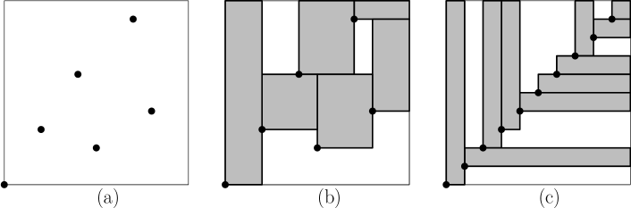
Figure 1: (a) A set $S$ of 6 points in a unit square $[0,1]^{2}$, including the origin $(0,0)$. (b) A rectangle packing where the lower left corner of each rectangle is a point in $S$. (c) Ten equally spaced points along the diagonal $[(0,0),(1,1)]$, and a corresponding rectangle packing that covers roughly 1/2 area.

Outline.

In this paper, we present two simple strategies for Bob that cover at least $0.09121$ area. These are the GreedyPacking and the TilePacking algorithms described below. Both algorithms process the points in the same specific order, namely the decreasing order of the sum of the two coordinates, with ties broken arbitrarily (hence $(0,0)$ is the last point processed).

The GreedyPacking algorithm chooses a rectangle of maximum area for each point in $S$ sequentially, in the above order.

The TilePacking algorithm partitions $U$ into staircase-shaped tiles, and then chooses a rectangle of maximum area within each tile independently. We next describe how the tiling is obtained. Each tile is a staircase-shaped polygon, with a vertical left side, a horizontal bottom side, and a descending staircase connecting them. The lower left corner of each tile is a point in $S$. We say that the tile is anchored at that point. The algorithm maintains the invariant that the set of unprocessed points are in the interior of a staircase shaped polygon (super-tile), and in addition the anchor and possibly other points are on its left and lower sides. Processing a point amounts to shooting a horizontal ray to the right and a vertical ray upwards which together isolate a new tile anchored at that point, and the new staircase shaped polygon containing the remaining points is updated. Since $(0,0)\in S$, TilePacking does indeed compute a tiling of the unit square.

It will be shown shortly (Lemma 2.1) that the GreedyPacking algorithm covers at least as much area as TilePacking. Hence it suffices to analyze the performance of the latter. The bulk of the work is in the analysis of this simple TilePacking algorithm, which involves geometric considerations and a charging scheme.

Related work.

Very little is known about anchored rectangle packing. Recently, Christ et al. [9] proved that if Alice can force Bob’s share to be less than $\frac{1}{r}$, then $n\geq 2^{2^{\Omega(r)}}$. Our result indicates that this condition does not materialize for large $r$, since Bob can always cover at least a constant fraction of the area for any $n\in\mathbb{N}$.

Previous results on rectangle packing typically consider optimization problems, and are only loosely related to our work. While our focus here is not on the optimization version of the anchored rectangle packing problem, in which the total area of the anchored rectangles is to be maximized for a given set $S$ of anchors, our algorithms do provide a constant-factor approximation.

In the classical strip packing problem, $n$ given axis-aligned rectangles should be placed (without rotation or overlaps) in a rectangular container of width 1 and minimum height. This problem is APX-hard (by a reduction from bin packing). After a series of previous results (e.g., [17, 18]), Harren et al. [12] recently found a $(5/3+\varepsilon)$-approximation. Jensen and Solis-Oba [14] devised an AFPTAS which packs the rectangles into a box of height at most $(1+\varepsilon){\rm OPT}+1$ for every $\varepsilon>0$. Bansal et al. [5] gave a 1.69-approximation algorithm for the 3-dimensional version.

Further related problems are the 2-dimensional knapsack and bin packing problems. Given a set of axis-aligned rectangles and a box $B$, the geometric 2D knapsack problem asks for a subset of the rectangles of maximum total area that fit into $B$. In contrast, the 2D bin packing asks for the minimum number of bins congruent to $B$ that can accommodate all rectangles. Jansen and Prädel [16] designed a PTAS for the geometric 2D knapsack problem, although it does not admit a FPTAS. The weighted version does not admit an AFPTAS and an approximation algorithm by Jansen and Zhang [15] guarantees a ratio of $2+\varepsilon$ for every $\varepsilon>0$. For the 2D bin packing, Jansen et al. [13] gave a 2-approximation, and Bansal et al. [3] designed a randomized algorithm with an asymptotic approximation ratio of about $1.525$, improving the previous ratio $1.691$ by Caprara [6, 7]. However, 2D bin packing does not admit an AFPTAS [4, 8]. Finally, we mention that Bansal et al. [4] gave a PTAS for the rectangle placement problem, which goes back to Erdős and Graham [11]. Here a given set of axis-aligned rectangles should be arranged (without rotation or overlaps) so that the area of their bounding box is minimized.

2 Constructing a rectangle packing

In this section we describe the two strategies for Bob and then compare their performance.

Ordering the points in $S$.

Let $S$ be a set of $n$ distinct points in the unit square $[0,1]^{2}$ such that $(0,0)\in S$. Denote by $x(s)$ and $y(s)$, respectively, the $x$- and $y$-coordinates of each point $s\in S$. Order the points in $S$ as $s_{1},s_{2},\ldots,s_{n}$ such that

$$x(s_{j})+y(s_{j})\leq x(s_{i})+y(s_{i})$$

for $1\leq i<j\leq n$ (ties are broken arbitrarily). Equivalently, this order is given by a left-moving sweep-line with slope $-1$. See Fig. 2. Clearly, we have $s_{n}=(0,0)$. In GreedyPacking, Bob chooses rectangles of maximum area for $s_{1},\ldots,s_{n}$ in this order.

GreedyPacking. For $i=1,\ldots,n$, choose an axis-aligned rectangle $r_{i}\subseteq[0,1]^{2}$ of maximum area such that the lower left corner of $r_{i}$ is $s_{i}$, and $r_{i}$ is interior-disjoint from any $r_{j}$, $j<i$.

Recall the partial order, called dominance order, among points in the plane. For two points, $p=(x_{p},y_{p})$ and $q=(x_{q},y_{q})$, we say that $p\preceq q$ (in words, $q$ dominates $p$) if

$$x_{p}\leq x_{q}\hskip 28.45274pt\mbox{\rm and}\hskip 28.45274pty_{p}\leq y_{q}.$$

With this definition, an axis-aligned rectangle with lower left corner $c_{1}$ and upper right corner $c_{2}$ can be written as $\{p\in\mathbb{R}^{2}:c_{1}\preceq p\preceq c_{2}\}$. In particular, any point in $r(s)$ dominates $s$.

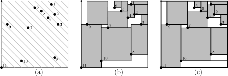
Figure 2: (a) Eleven points in $[0,1]^{2}$, sorted by decreasing order of the sum of coordinates. (b) Rectangles chosen greedily in this order. (c) The tiling of $[0,1]^{2}$ induced by the dominance order; and the maximum-area rectangles chosen from each tile. Note that rectangle 8 is smaller than the corresponding greedy rectangle.

We now define interior-disjoint tiles for the set $S=\{s_{1},\ldots,s_{n}\}$ that jointly cover the unit square $U=[0,1]^{2}$. For $i=1,2,\ldots,n$, let tile $t_{i}$ be the set of points in $U$ that dominate $s_{i}$, but have not been covered by any previous tile $t_{j}$, $j<i$. Formally, let

$$t_{i}=\{p\in[0,1]^{2}:s_{i}\preceq p\mbox{ \rm and }s_{j}\not\preceq p\mbox{ \rm for all }j<i\}.$$

The tiles are disjoint by definition, and they cover $U$ since the origin is in $S$. Each tile is a staircase polygon with axis-aligned sides, bounded by one horizontal side from below, one vertical side from the left, and a monotone decreasing curve from the top and from the right. Observe that the axis-aligned rectangle spanned by the lower left corner $s_{i}$ and any point $p\in t_{i}$ is contained in the tile $t_{i}$. That means that every maximum-area axis-aligned rectangle in the tile is incident to the lower left corner $s_{i}$. We can now describe our second strategy for Bob.

TilePacking. Compute the tiling $U=\bigcup_{i=1}^{n}t_{i}$. For $i=1,\ldots,n$, independently, choose an axis-aligned rectangle $r_{i}\subseteq t_{i}$ of maximum area.

By the above observation, the lower left corner of $r_{i}$ is the lower left corner of the tile $t_{i}$, which is $s_{i}\in S$.

We now show that GreedyPacking always covers a greater or equal area than TilePacking.

Lemma 2.1

For each point $s_{i}\in S$, GreedyPacking chooses a rectangle of greater or equal area than TilePacking.

Proof 2.2

The rectangles chosen by the greedy tiling for $s_{j}$, $j<i$, are all disjoint from the tile $t_{i}$, because every point in $r(s_{j})$ dominates $s_{j}$. Hence, GreedyPacking could choose any maximum-area axis-aligned rectangle from tile $t_{i}$, but it may choose a larger rectangle (such as $r(s_{8})$ in Fig. 2).

Remark.

It is worth noting that GreedyPacking cannot give a better worst-case constant than TilePacking. If $S$ is in ”general position” (that is, no two points lie on the same sweep-line), we construct a set $S^{\prime}$, where $|S^{\prime}|\leq 3n-2$ as follows. Choose a sufficiently small $\varepsilon>0$. Then for each point $s_{i}=(x_{i},y_{i})$ in the interior of $U$, we add two nearby points $(x_{i}-\varepsilon,y_{i})$ and $(x_{i},y_{i}-\varepsilon)$ (below the sweep-line incident to $s_{i}$, one to the left of $s_{i}$ and one below $s_{i}$). Observe that on input $S^{\prime}$, GreedyPacking and TilePacking give the same set of rectangles. Moreover, the total area covered by TilePacking with $S^{\prime}$ and the total area covered by TilePacking with $S$ will differ from each other by an arbitrarily small amount, i.e., by at most $2n\varepsilon$.

3 Analysis of TilePacking

Formally, define $\rho$ as the worst-case performance of TilePacking. In this section, we show that TilePacking chooses a set of rectangles of total area $\rho\geq 0.09121$. In our analysis, we will use two variables, $\beta\geq 5$ and $0<\lambda<1$.

Let $r_{i}\subseteq t_{i}$ be the axis-aligned rectangle of maximum area in tile $t_{i}$, whose lower left corner is $s_{i}$, and let $R=\{r_{i}:i=1,\ldots,n\}$ be this set of rectangles. If ${\rm area}(r_{i})\geq 0.09121\cdot{\rm area}(t_{i})$ for every $i$, then our proof is complete. However, the ratio ${\rm area}(r_{i})/{\rm area}(t_{i})$ may be arbitrarily small because the tiles can be arbitrary staircase polygons.

For $\beta\geq 5$, we say that tile $t_{i}$ is a $\beta$-tile if ${\rm area}(r_{i})<\frac{1}{\beta}\ {\rm area}(t_{i})$. We will give an upper bound $F(\beta,\lambda)$ on the total area of $\beta$-tiles for every $\beta\geq 5$ and $0<\lambda<1$. This immediately implies that, for every $\beta\geq 5$, the complement of all $\beta$-tiles cover at least $1-F(\beta,\lambda)$ area, and the total area of all rectangles in $R$ is

$$\sum_{i=1}^{n}{\rm area}(r_{i})\geq\rho\geq\frac{1-F(\beta,\lambda)}{\beta}.$$ (1)

In Section 3.1 we study the properties of individual $\beta$-tiles, and in Section 3.2 we prove an upper bound on the total area of $\beta$-tiles (for every $\beta\geq 5$), which already gives a preliminary bound $\rho\geq 0.07229$, using (1). By integrating over $\beta$, we improve this bound to $\rho\geq 0.09121$ in Section 3.3. Finally, Section 3.4 shows that TilePacking runs in $O(n\log n)$ time.

3.1 Properties of a $\beta$-tile

Let us introduce some notation for describing a single tile $t_{i}$ (Fig. 3(a)). It is bounded from below by a horizontal side, denoted $a_{i}$, and from the left by a vertical side, denoted $b_{i}$. The width (resp., height) of $t_{i}$ is the length of $a_{i}$ (resp., $b_{i}$), denoted by $|a_{i}|$ (resp., $|b_{i}|$). We show next that a $\beta$-tile $t_{i}$ has a much smaller area than its bounding box (recall that $\beta$-tiles are defined for $\beta\geq 5$).

Lemma 3.1

Let $\beta\geq 1$ and $t$ be a staircase polygon of height $h$ and width $w$. If the area of every axis-aligned rectangle contained in $t$ is less than ${\rm area}(t)/\beta$, then

$${\rm area}(t)<\frac{\beta}{e^{\beta-1}}\cdot hw,$$ (2)

and this bound is the best possible.

Proof 3.2

Assume, by translating $t$ if necessary, that the lower left corner of $t$ is the origin. Then the bounding box of $t$ is $[0,w]\times[0,h]$. Let ${\rm area}(t_{i})=\beta u^{2}$, for some $u>0$. Then all vertices of $t$ lie strictly below the hyperbola arc $f(x)=u^{2}/x$, for $0<x$. See Fig. 3(b). The area of the part of $[0,w]\times[0,h]$ below the curve $f(x)=u^{2}/x$ is

$$u^{2}+\int_{u^{2}/h}^{w}\frac{u^{2}}{x}\ {\rm d}x=u^{2}+\big{[}u^{2}\ln x\big{]}_{u^{2}/h}^{w}=u^{2}(1+\ln w-\ln(u^{2}/h))=u^{2}(1+\ln(hw)-\ln u^{2}).$$

We have shown that ${\rm area}(t)=\beta u^{2}<u^{2}(1+\ln(hw)-\ln u^{2})$, or $\beta<1+\ln(hw)-\ln u^{2}$. Rearranging this inequality yields $e^{\beta-1}u^{2}<hw$, which implies (2), as required.

If we approximate the shaded area in Fig. 3(b) with a staircase polygon $t$ of height $h$ and width $w$ that lies strictly below the hyperbola, then the area of every axis-aligned rectangle contained in $t$ is less than $u^{2}$, and ${\rm area}(t)$ can be arbitrarily close to $\frac{\beta}{e^{\beta-1}}\cdot hw$.

Sectors and tips.

Fix $\beta\geq 5$ and consider a $\beta$-tile $t_{i}$. Decompose $t_{i}$ into rectangular vertical sectors by vertical lines passing though its vertices; see Fig. 3(c). Each sector is part of some maximum-area axis-aligned rectangle in $t_{i}$. Hence the area of each sector is less than ${\rm area}(t_{i})/\beta$, where near equality is possible for the leftmost sector. Similarly, we can decompose $t_{i}$ into rectangular horizontal sectors by horizontal lines passing through its vertices, and the area of each sector is less than ${\rm area}(t_{i})/\beta$.

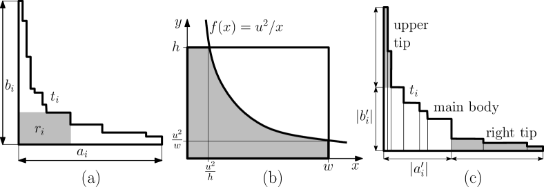
Figure 3: (a) A $\beta$-tile $t_{i}$ of width $|a_{i}|$ and height $|b_{i}|$. (b) The portion of the rectangle $[0,w]\times[0,h]$ below the hyperbola arc $f(x)=u^{2}/x$. (c) The decomposition of $t_{i}$ into vertical sectors. The tips of $t_{i}$ are shaded.

Decompose each $\beta$-tile $t_{i}$ into three parts, called right tip, upper tip, and main body, as follows. The right tip of $t_{i}$ is cut off from $t_{i}$ by the right-most vertical line that passes through a vertex of $t_{i}$ such that the area of the right part is at least ${\rm area}(t_{i})/\beta$. Similarly, the upper tip of $t_{i}$ is cut off from $t_{i}$ by the upper-most horizontal line that passes through a vertex of $t_{i}$ such that the area of the part above is at least ${\rm area}(t_{i})/\beta$. The remaining part, denoted by $t_{i}^{\prime}$, is the main body of $t_{i}$. All three parts are staircase polygons. Both the right and the upper tips are unions of some sectors of $t_{i}$. Since the area of each sector is less than ${\rm area}(t_{i})/\beta$, the area of each tip is at least $\frac{1}{\beta}{\rm area}(t_{i})$ but less than $\frac{2}{\beta}{\rm area}(t_{i})$. In particular, since $\beta\geq 5$, the right tip of $t_{i}$ is disjoint from the upper tip of $t_{i}$.

Let $a_{i}^{\prime}$ and $b_{i}^{\prime}$, respectively, be the lower and left side of $t_{i}^{\prime}$. Note that the topmost horizontal side and the rightmost vertical side of $t_{i}^{\prime}$ each contains some point from $S$, because each contains a reflex vertex of the original tile $t_{i}$.

Lemma 3.3

The width of the right tip of $t_{i}$ is at least $|a_{i}^{\prime}|$, hence $2|a_{i}^{\prime}|\leq|a_{i}|$. Similarly, the height of the upper tip of $t_{i}$ is at least $|b_{i}^{\prime}|$, hence $2|b_{i}^{\prime}|\leq|b_{i}|$.

Proof 3.4

By symmetry, it is enough to prove the first claim. Let $r^{\prime}$ be the maximum-area axis-aligned rectangle in $t_{i}$ whose lower side is $a_{i}^{\prime}$. Since $t_{i}$ is a $\beta$-tile, the area of $r^{\prime}$ is less than $\frac{1}{\beta}{\rm area}(t_{i})$. Recall that the area of each tip is at least $\frac{1}{\beta}{\rm area}(t_{i})$, thus ${\rm area}(r^{\prime})$ is less than the area of the right tip of $t_{i}$, and so ${\rm area}(r^{\prime})$ is less than the area of the bounding box of the right tip of $t_{i}$. However, the height of $r^{\prime}$ is strictly greater than the height of the right tip (and its bounding box). Therefore, the width of $r^{\prime}$, which is $|a_{i}^{\prime}|$, is less than the width of the right tip of $t_{i}$. Thus $|a_{i}^{\prime}|\leq|a_{i}|-|a_{i}^{\prime}|$, or $2|a_{i}^{\prime}|\leq|a_{i}|$, as required.

Recall that the areas of the right and upper tips of $t_{i}$ are each less than $\frac{2}{\beta}{\rm area}(t_{i})$. Hence ${\rm area}(t_{i})<\frac{\beta}{\beta-4}{\rm area}(t_{i}^{\prime})$. Since $t_{i}$ is a $\beta$-tile and $t_{i}^{\prime}\subset t_{i}$, the area of every axis-aligned rectangle contained in $t_{i}^{\prime}$ is less than ${\rm area}(t_{i})/\beta<{\rm area}(t_{i}^{\prime})/(\beta-4)$. Applying Lemma 3.1 for the main body $t_{i}^{\prime}$ yields

$${\rm area}(t_{i})<\frac{\beta}{\beta-4}\cdot{\rm area}(t_{i}^{\prime})<\frac{\beta}{\beta-4}\cdot\frac{\beta-4}{e^{\beta-5}}\cdot|a_{i}^{\prime}|\cdot|b_{i}^{\prime}|=\frac{\beta}{e^{\beta-5}}\cdot|a_{i}^{\prime}|\cdot|b_{i}^{\prime}|.$$ (3)

Tall and wide tiles.

We distinguish two types of $\beta$-tiles based on the height and width of their main body. A $\beta$-tile $t_{i}$ is tall if $|a_{i}^{\prime}|<|b_{i}^{\prime}|$; and it is wide if $|a_{i}^{\prime}|\geq|b_{i}^{\prime}|$. For wide $\beta$-tiles, we have $\max(|a_{i}^{\prime}|,|b_{i}^{\prime}|)=|a_{i}^{\prime}|$, and (3) implies

$${\rm area}(t_{i})<\frac{\beta}{e^{\beta-5}}|a_{i}^{\prime}|^{2}.$$ (4)

Similarly, if a $\beta$-tile $t_{i}$ is tall, then ${\rm area}(t_{i})<\frac{\beta}{e^{\beta-5}}|b_{i}^{\prime}|^{2}$.

3.2 Upper bound on the total area of $\beta$-tiles

In this section we give an upper bound $F(\beta,\lambda)$ (see equation (10) further bellow) on the total area of all $\beta$-tiles for every $\beta\geq 5$ and $0<\lambda<1$. It is enough to bound the total area of wide $\beta$-tiles by $\frac{1}{2}F(\beta,\lambda)$. By symmetry, the same upper bound holds for the total area of tall $\beta$-tiles. Let $W\subset\{1,\ldots n\}$ be the set of indices of the wide $\beta$-tiles.

To begin, for every tile $t_{i}$ we define two adjacent triangles. Let $\Delta_{i}$ be the isosceles right triangle bounded by $a_{i}$, the line of slope $-1$ through $s_{i}$, and a vertical line through the right endpoint of $a_{i}$ (see Fig. 4(a)). Similarly, let $\Gamma_{i}$ be isosceles right triangle adjacent to $b_{i}$ that lies left of $t_{i}$. The two triangles $\Delta_{i}$ and $\Gamma_{i}$ are not part of the tiling $\{t_{i}:i=1\ldots n\}$, and they may intersect several tiles. A key fact is that these two triangles are empty of points from $S$ in their interior, regardless whether the tile $t_{i}$ is a $\beta$-tile or not.

Lemma 3.5

For every $i=1,\ldots,n$, the interior of $\Delta_{i}$ (resp., $\Gamma_{i}$) is disjoint from $S$.

Proof 3.6

Suppose to the contrary, that there exist points in $S$ in the interior of $\Delta_{i}$, and let $s_{j}$ be the first such point processed by the algorithm. Then $s_{j}$ is processed before $s_{i}$, and so the left side $b_{j}$ of the tile $t_{j}$ would cut through the horizontal segment $a_{i}$, which is a contradiction. Similarly, if $s_{j}$ lies in the interior of $\Gamma_{i}$, then the lower side $a_{j}$ would cut through the left side $b_{i}$.

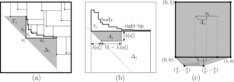
Figure 4: (a) Tiles $t_{1},\ldots,t_{i}$, and the triangles $\Delta_{i}$ and $\Gamma_{i}$. (b) The trapezoid $A_{i}\subset\Delta_{i}$. (c) Every trapezoid $A_{i}$ is contained in the shaded (hexagonal) region.

We charge the area of each wide $\beta$-tile $t_{i}$ to the trapezoid $A_{i}\subset\Delta_{i}$ defined below. Let $A_{i}$ be the set of points in $\Delta_{i}$ that lie vertically below the segment $a_{i}^{\prime}$ at distance at most $\lambda|a_{i}^{\prime}|$ from it. See Fig. 4(c). Using Inequality (4), the area of $A_{i}$ can be bounded from below as follows in terms of the area of $t_{i}$:

$${\rm area}(A_{i})=\frac{|a_{i}^{\prime}|+(1-\lambda)|a_{i}^{\prime}|}{2}\cdot\lambda|a_{i}^{\prime}|=\frac{\lambda(2-\lambda)}{2}\cdot|a_{i}^{\prime}|^{2}>\frac{\lambda(2-\lambda)\cdot e^{\beta-5}}{2\beta}\cdot{\rm area}(t_{i}).$$ (5)

The trapezoids $A_{i}$, $i\in W$, are homothetic copies of each other, and their area depends only on $|a_{i}^{\prime}|$. Note that the triangles $\Delta_{i}$ (and also the trapezoids $A_{i}$) may extend beyond the boundary of $U=[0,1]^{2}$ (e.g., in Fig. 4(b), $\Delta_{i}$ extends below $U$). We show that all trapezoids $A_{i}$, $i\in W$, lie in a polygon whose area is at most $1+\lambda(3-\lambda)/8$.

Lemma 3.7

Every trapezoid $A_{i}$, $i\in W$, lies in a polygon of area $1+\lambda(3-\lambda)/8$.

Proof 3.8

Every trapezoid $A_{i}$ lies vertically below a segment $a_{i}^{\prime}$, which is part of the lower side of tile $t_{i}$. Therefore, $A_{i}$ cannot extend beyond the left, right, and upper sides of the unit square $U$. Moreover, we show that $A_{i}$ is contained in the shaded polygon in Fig. 4(c).

Consider a trapezoid $A_{i}$, and the corresponding lower side $a_{i}$ of a $\beta$-tile $t_{i}$, $i\in W$. Translate them vertically down until $a_{i}$ lies on the $x$-axis. Then apply a dilation centered at the right endpoint of $a_{i}$ (now on the $x$-axis), such that the left endpoint of $a_{i}$ becomes $(0,0)$. Finally, apply a dilation centered at $(0,0)$ such that the right endpoint of $a_{i}$ becomes $(1,0)$. Observe that through all three transformations, the trapezoid $A_{i}$ remains in the shaded polygon. The shaded polygon is the union of $U$ and a trapezoid of area $\frac{1}{2}(1+\frac{1-\lambda}{2})\frac{\lambda}{2}=\lambda(3-\lambda)/8$.

The case of pairwise disjoint trapezoids.

If the trapezoids $A_{i}$, for all $i\in W$, are pairwise disjoint, then we can deduce an upper bound for the total area of wide $\beta$-tiles: By Lemma 3.7, we have

$$\sum_{i\in W}{\rm area}(A_{i})\leq 1+\frac{\lambda(3-\lambda)}{8}=\frac{8+3\lambda-\lambda^{2}}{8}.$$

Using Inequalities (4) and (5), this implies

$$\sum_{i\in W}{\rm area}(t_{i})<\frac{8+3\lambda-\lambda^{2}}{8}\cdot\frac{2\beta}{\lambda(2-\lambda)\cdot e^{\beta-5}}=\frac{(8+3\lambda-\lambda^{2})}{4\lambda(2-\lambda)}\cdot\frac{\beta}{e^{\beta-5}}.$$ (6)

The general case of overlapping trapezoids.

However, it is possible that the trapezoids $A_{i}$, $i\in W$, are not disjoint. To take care of this possibility, we set up a charging scheme, in which we choose a set of “large” pairwise disjoint trapezoids. For every trapezoid $A_{i}$, $i\in W$, denote by $\ell_{i}$ the supporting line of $a_{i}$. We say that $A_{i}$ is above $A_{j}$ (and $A_{j}$ is below $A_{i}$) if $A_{i}$ and $A_{j}$, $i\neq j$ and $\ell_{i}$ is above $\ell_{j}$. We next show that if $A_{i}$ and $A_{j}$ overlap, then the trapezoid below the other is significantly larger.

Lemma 3.9

Assume that $A_{i}\cap A_{j}\neq\emptyset$, for some $i,j\in W$, $i\neq j$; and $A_{i}$ is above $A_{j}$. Then $\ell_{j}\cap\Delta_{i}\subseteq a_{j}^{\prime}$ and $(2-\lambda)|a_{i}^{\prime}|\leq|a_{j}^{\prime}|$.

Proof 3.10

Refer to Fig. 5(a). If $A_{i}\cap A_{j}\neq\emptyset$, and line $\ell_{i}$ is above line $\ell_{j}$, then the segment $a_{j}^{\prime}$ has to intersect $A_{i}$. Note that the left endpoint of $a_{j}^{\prime}$ is $s_{j}\in S$, and there is some point from $S$ on the rightmost edge of $t_{j}^{\prime}$. By Lemma 3.5, however, there is no point from $S$ in the interior of $\Delta_{i}$. Therefore, $a_{j}^{\prime}$ has to traverse both $A_{i}$ and $\Delta_{i}$, hence $\ell_{j}\cap\Delta_{i}\subseteq a_{j}^{\prime}$.

The minimum horizontal cross-section of $A_{i}$ is $(1-\lambda)|a_{i}^{\prime}|$, and the width of the right tip of $t_{i}$ is at least $|a_{i}^{\prime}|$ by Lemma 3.3. It follows that $|a_{j}^{\prime}|\geq|\ell_{j}\cap\Delta_{i}|\geq(1-\lambda)|a_{i}^{\prime}|+|a_{i}^{\prime}|=(2-\lambda)|a_{i}^{\prime}|$.

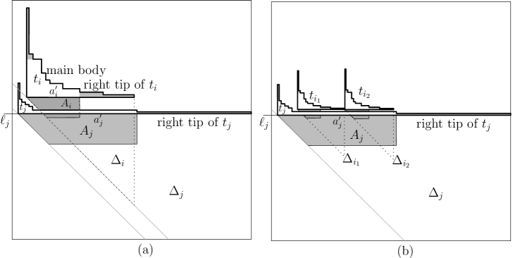
Figure 5: (a) If $A_{i}$ and $A_{j}$ overlap, and $a_{j}$ lies below $a_{i}$, then $|a_{j}^{\prime}|\geq(2-\lambda)|a_{i}^{\prime}|$. (b) Trapezoids $A_{i_{1}}$ and $A_{i_{2}}$ intersect $A_{j}$ from above such that the intervals $a_{j}^{\prime}\cap\Delta_{i_{1}}$ and $a_{j}^{\prime}\cap\Delta_{i_{2}}$ are disjoint.

Charging scheme.

We introduce a charging scheme among the trapezoids $A_{i}$, $i\in W$. Initially, each trapezoid $A_{i}$ has a charge of ${\rm area}(A_{i})$. We transfer the charges to a subset of pairwise disjoint trapezoids. The transfer of charges is represented by a directed acyclic graph $G$ defined as follows. The nodes of $G$ correspond to the trapezoids $A_{i}$, $i\in W$. If $A_{i}$ intersects some other trapezoid below, we add a unique outgoing edge from $A_{i}$ to the trapezoid $A_{j}$, $j\in W$, whose top side $a_{j}^{\prime}$ is the highest below $a_{i}^{\prime}$. Observe that all edges of $G$ are oriented downwards, thus $G$ is acyclic. By construction, the out-degree of $G$ is at most one. However, the in-degree of a node in $G$ may be higher than one.

Lemma 3.11

For every trapezoid $A_{j}$, the total area of all trapezoids $A_{i}$, $i\neq j$, with a directed path in $G$ to $A_{j}$ is at most $\frac{1}{(1-\lambda)(2-\lambda)}{\rm area}(A_{j})$.

Proof 3.12

Fix a trapezoid $A_{j}$, $j\in W$, and denote by $\ell_{j}$ be the supporting line of $a_{j}$. Refer to Fig. 6(a). For $k\geq 1$, let $W_{j}^{k}\subseteq W$ be the set of indices $i$ of trapezoids $A_{i}$ that have a directed path of length exactly $k$ to $A_{j}$ in $G$. We say that the trapezoids $A_{i}$, $i\in W_{j}^{k}$ are on level $k$. In particular, the trapezoids $A_{i}$, $i\in W_{j}^{1}$, on level 1 are connected to $A_{j}$ with a directed edge $(A_{i},A_{j})\in G$. Let $W_{j}=\bigcup_{k\geq 1}W_{j}^{k}$ be the set of indices of all trapezoids $A_{i}$, $i\neq j$, with a directed path in $G$ to $A_{j}$. For each $A_{i}$, $i\in W_{j}$, denote by $A_{i}^{*}$ the unique trapezoid with $(A_{i},A_{i}^{*})\in G$.

By Lemma 3.9, every trapezoid $A_{i}$, $i\in W_{j}^{1}$, has width at most $|a_{i}^{\prime}|\leq|a_{j}^{\prime}|/(2-\lambda)$, and height at most $\frac{\lambda}{2-\lambda}|a_{j}^{\prime}|$. Equality is possible if the lower left corner of $A_{i}$ coincides with the upper left corner $s_{j}$ of $A_{j}$ (see $A_{i_{1}}$ in Fig. 6(a)). The gray triangle in Fig. 6(a) is the minimum triangle with base $a_{j}^{\prime}$ that contains the maximal possible trapezoid intersecting $A_{j}$ from above. By triangle similarity, the height of this triangle is $\frac{\lambda}{1-\lambda}|a_{j}^{\prime}|$, hence its area is (using Equation (5))

$$\frac{1}{2}\cdot|a_{j}^{\prime}|\cdot\frac{\lambda}{1-\lambda}|a_{j}^{\prime}|=\frac{\lambda}{2(1-\lambda)}|a_{j}^{\prime}|^{2}=\frac{{\rm area}(A_{j})}{(1-\lambda)(2-\lambda)}.$$ (7)

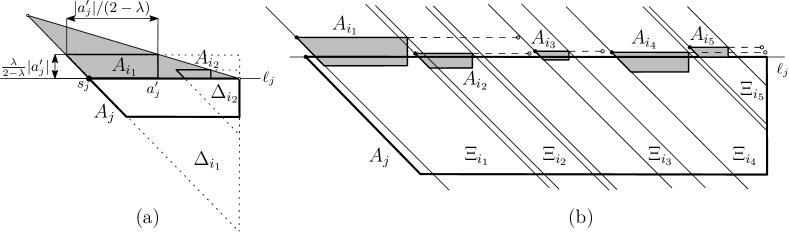
Figure 6: (a) $A_{i_{1}}$ is the largest possible trapezoid that can intersect $A_{j}$ from above. All trapezoids with a directed path in $G$ to $A_{j}$ can be translated (without overlaps) into the gray triangle. (b) Disjoint trapezoids $A_{i_{1}}\ldots,A_{i_{5}}$ intersect $A_{j}$ from above. Each of these trapezoids induces a parallel strip $\Xi_{i}$. If the strips $\Xi_{i_{1}}$ and $\Xi_{i_{2}}$ intersect, and $A_{i_{1}}$ is above $A_{i_{2}}$, then $s_{i_{2}}$ lies in the interior of $\Delta_{i_{1}}$. Dashed lines indicate segments $a_{i}\setminus a_{i}^{\prime}$.

We claim that $\sum_{i\in W_{j}}{\rm area}(A_{i})$ is at most the area of the gray triangle in Figure 6(a). To verify the claim, we translate every trapezoid $A_{i}$, $i\in W_{j}$, into the gray triangle region such that they remain pairwise disjoint. Each trapezoid will be translated in the same direction, $(-1,1)$, but at different distances. In order to control the possible location of the translates, we enclose each $A_{i}$, $i\in W_{j}$, in a parallel strip. For every $i\in W_{j}$, draw lines of slope $-1$ through the two endpoints of $a_{i}^{\prime}$, and denote by $\Xi_{i}$ the strip bounded by the two lines. Refer to Fig. 6(b).

First consider the trapezoids $A_{i}$, $i\in W_{j}^{1}$, which are connected to $A_{j}$ by a directed edge in $G$. By the definition of $G$, the trapezoids $A_{i}$, $i\in W_{j}^{1}$, are pairwise disjoint. Label their strips in increasing order from left to right. We show that the strips $\Xi_{i}$, $i\in W_{j}^{1}$, are pairwise interior-disjoint. Suppose to the contrary that $\Xi_{i_{1}}$ and $\Xi_{i_{2}}$ intersect, where ${i_{1}}<{i_{2}}$, and such that $A_{i_{1}}$ is above $A_{i_{2}}$ (if $A_{i_{1}}$ is below $A_{i_{2}}$, the strips are obviously disjoint). Since the trapezoids are disjoint, the left endpoint of $a_{i_{2}}^{\prime}$, $s_{i_{2}}\in S$, lies in the interior of the isosceles right triangle bounded by the right side of $A_{i_{1}}$, line $\ell_{j}$, and the line of slope $-1$ bounding the strip $\Xi_{i_{1}}$ from the right. Since $\lambda<1$ and $|a_{i_{1}}|-|a_{i_{1}}^{\prime}|\geq|a_{i_{1}}^{\prime}|$ by Lemma 3.3, this triangle is contained in $\Delta_{i_{1}}$. However, the triangle $\Delta_{i_{1}}$ is empty of points from $S$, and we reached a contradiction.

Applying the above argument for the trapezoids on level $k$, $k=1,2,\ldots$, we conclude that the trapezoids on level $k+1$ are pairwise disjoint, and they induce pairwise disjoint parallel strips.

We are now ready to describe the translation of the trapezoids $A_{i}$, $i\in W_{j}$. We translate the trapezoids in direction $(-1,1)$ in phases $k=1,2,\ldots$. In phase $k$, consider each $A_{i}$, $i\in W_{j}^{k}$, independently. Translate $A_{i}$ together with all other trapezoids that have a directed path to $A_{i}$ by the same vector in direction $(-1,1)$ until the lower side of $A_{i}$ becomes collinear with the upper side of $A_{i}^{*}$. Each trapezoid $A_{i}$ remains in its parallel strip $\Xi_{i}$, therefore the trapezoids on the same level remain pairwise disjoint. After phase $k$, there is no overlap between a trapezoid $A_{i}$, $i\in W_{j}^{k}$ of level $k$ and trapezoids in lower levels. When all phases are complete, all trapezoids are pairwise interior-disjoint.

It remains to show that after the translation, all trapezoids lie in the gray triangle in Fig. 6(a). From Lemma 3.9 and since all translations were done in direction $(-1,1)$, the trapezoids are on or to the right of the line of slope $-1$ passing through $s_{j}$. Also from Lemma 3.9, the right endpoint of $a_{j}^{\prime}$ is to the right of the right side of every triangle $\Delta_{i}$, $i\in W_{j}^{1}$, hence to the right of the right side of every triangle $\Delta_{i}$, $i\in W_{j}$. Also, if $i\in W_{j}^{1}$, by Lemma 3.3 we have $2|a_{i}^{\prime}|\leq|a_{i}|$, and so $\frac{\lambda|a_{i}^{\prime}|}{|a_{i}|-|a_{i}^{\prime}|}\leq\frac{\lambda|a_{i}^{\prime}|}{|a_{i}^{\prime}|}=\lambda$. Hence the upper right corner of every $A_{i}$, $i\in W_{j}^{1}$, is below the line of slope $-\lambda$ passing through the right endpoint of $a_{j}^{\prime}$, and consequently, the upper right corner of every $A_{i}$, $i\in W_{j}$, is below the line of slope $-\lambda$ passing through the right endpoint of $a_{j}^{\prime}$. Therefore, after the above translation, all trapezoids $A_{i}$, $i\in W_{j}$, are contained in the gray triangle in Figure 5(c). This verifies the above claim and completes the proof of the lemma.

Transfer the charges from all nodes to the sinks in $G$ along directed paths. By Lemma 3.11, the total area charged to a sink $A_{j}$ is less than

$${\rm area}(A_{j})+\frac{1}{(1-\lambda)(2-\lambda)}{\rm area}(A_{j})=\frac{3-3\lambda+\lambda^{2}}{(1-\lambda)(2-\lambda)}{\rm area}(A_{j})$$ (8)

The area of every trapezoid $A_{i}$, $i\in W$, is charged to some sink in $G$, and the sinks correspond to pairwise disjoint trapezoids. We can now adjust Inequality (6) to obtain

$$\sum_{i\in W}{\rm area}(t_{i})<\frac{3-3\lambda+\lambda^{2}}{(1-\lambda)(2-\lambda)}\cdot\frac{(8+3\lambda-\lambda^{2})}{4\lambda(2-\lambda)}\cdot\frac{\beta}{e^{\beta-5}}=\frac{(3-3\lambda+\lambda^{2})(8+3\lambda-\lambda^{2})}{4\lambda(1-\lambda)(2-\lambda)^{2}}\cdot\frac{\beta}{e^{\beta-5}}.$$ (9)

The area of all $\beta$-tiles is less than twice the right hand-side of (9), namely we can set

$$F(\beta,\lambda)=\frac{(3-3\lambda+\lambda^{2})(8+3\lambda-\lambda^{2})}{2\lambda(1-\lambda)(2-\lambda)^{2}}\cdot\frac{\beta}{e^{\beta-5}}.$$ (10)

From (1), it follows that the total area of all rectangles in $R$ is

$$\rho\geq\frac{1-F(\beta,\lambda)}{\beta} =\frac{1}{\beta}\left(1-\frac{(3-3\lambda+\lambda^{2})(8+3\lambda-\lambda^{2})}{2\lambda(1-\lambda)(2-\lambda)^{2}}\cdot\frac{\beta}{e^{\beta-5}}\right)$$

$$=\frac{1}{\beta}-\frac{(3-3\lambda+\lambda^{2})(8+3\lambda-\lambda^{2})}{2\lambda(1-\lambda)(2-\lambda)^{2}}\cdot\frac{1}{e^{\beta-5}}.$$

Whenever $F(\beta,\lambda)<1$, this already gives a lower bound of $\rho=\Omega(1)$. We have optimized the parameters $\beta$ and $\lambda$ with numerical methods. With the choice of $\beta=12.75$ and $\lambda=0.45$, we obtain an initial lower bound of $\rho\geq 0.07229$.

3.3 Making $\beta$ a continuous variable

In this section we further improve the lower bound on the covered area to $0.09121$ by making $\beta$ a continuous variable and using integration. We define the contribution of each point $p\in t_{i}\subseteq U$, as $u(p)={\rm area}(r_{i})/{\rm area}(t_{i})$. With this definition, we have

$$\sum_{i=1}^{n}{\rm area}(r_{i})=\iint_{p\in U}u(p)\ {\rm d}A.$$

Let $\beta_{0}\geq 5$ be a parameter to be optimized later (we will choose $\beta_{0}=9.955$). Partition the interval $[\beta_{0},\infty)$ into subintervals of length $\varepsilon>0$: $[\beta_{0},\infty)=\bigcup_{j=1}^{\infty}[\beta_{j-1},\beta_{j})$, where $\beta_{j}=\beta_{0}+j\varepsilon$. Denote by $B_{j}\subset U$ the union of all $\beta_{j}$-tiles, and let $\overline{B}_{j}=U\setminus B_{j}$. By definition, we have $u(P)\geq 1/\beta_{j}$ for every $p\in\overline{B}_{j}$, and so $\iint_{p\in\overline{B}_{j}}u(p)\ {\rm d}A\geq{\rm area}(\overline{B}_{j})/\beta_{j}$.

Observe that the sets $\overline{B}_{j}$ form a nested sequence $\overline{B}_{0}\subseteq\overline{B}_{1}\subseteq\overline{B}_{2}\subseteq\ldots\subseteq U$. The total contribution of all points in $U$ can be written as

$$\sum_{j=1}^{n}{\rm area}(r_{i}) = \iint_{p\in U}u(p)\ {\rm d}A$$

$$= \iint_{p\in\overline{B}_{0}}u(p)\ {\rm d}A+\sum_{j=1}^{\infty}\iint_{p\in\overline{B}_{j}\setminus\overline{B}_{j-1}}u(p)\ {\rm d}A$$

$$\geq \frac{{\rm area}(\overline{B}_{0})}{\beta_{0}}+\sum_{j=1}^{\infty}\frac{{\rm area}(\overline{B}_{j}\setminus\overline{B}_{j-1})}{\beta_{j}}$$

$$= \frac{{\rm area}(\overline{B}_{0})}{\beta_{0}}+\sum_{j=1}^{\infty}\frac{{\rm area}(\overline{B}_{j})-{\rm area}(\overline{B}_{j-1})}{\beta_{j}}$$

$$= \sum_{j=0}^{\infty}{\rm area}(\overline{B}_{j})\left(\frac{1}{\beta_{j}}-\frac{1}{\beta_{j+1}}\right).$$

In Section 3.2, we showed that for any $j\geq 0$, ${\rm area}(B_{j})<F(\beta_{j},\lambda)$, where $F(\beta,\lambda)$ is given by (10). It follows that ${\rm area}(\overline{B}_{j})>1-F(\beta_{j},\lambda)$, and therefore,

$$\rho \geq \sum_{j=0}^{\infty}(1-F(\beta_{j},\lambda))\left(\frac{1}{\beta_{j}}-\frac{1}{\beta_{j+1}}\right)$$

$$= \frac{1-F(\beta_{0},\lambda)}{\beta_{0}}+\sum_{j=0}^{\infty}\frac{(1-F(\beta_{j+1},\lambda))-(1-F(\beta_{j},\lambda))}{\beta_{j+1}}$$

$$= \frac{1-F(\beta_{0},\lambda)}{\beta_{0}}+\sum_{j=0}^{\infty}\frac{F(\beta_{j},\lambda)-F(\beta_{j+1},\lambda)}{\beta_{j+1}}$$

$$= \frac{1-F(\beta_{0},\lambda)}{\beta_{0}}-\sum_{j=0}^{\infty}\frac{1}{\beta_{j+1}}\cdot\frac{F(\beta_{j+1},\lambda)-F(\beta_{j},\lambda)}{\beta_{j+1}-\beta_{j}}\cdot(\beta_{j+1}-\beta_{j}).$$

Letting $\varepsilon$ go to 0 yields

$$\rho \geq \frac{1-F(\beta_{0},\lambda)}{\beta_{0}}-\int_{\beta_{0}}^{\infty}\left(\frac{1}{\beta}\cdot\frac{\partial}{\partial\beta}F(\beta,\lambda)\right){\rm d}\beta$$

$$= \frac{1}{\beta_{0}}+\frac{(3-3\lambda+\lambda^{2})(8+3\lambda-\lambda^{2})}{2\lambda(1-\lambda)(2-\lambda)^{2}}e^{5}\left(-\frac{1}{e^{\beta_{0}}}-\int_{\beta_{0}}^{\infty}\left(\frac{1}{\beta}\cdot\frac{{\rm d}}{{\rm d}\beta}\frac{\beta}{e^{\beta}}\right){\rm d}\beta\right)$$

$$= \frac{1}{\beta_{0}}+\frac{(3-3\lambda+\lambda^{2})(8+3\lambda-\lambda^{2})}{2\lambda(1-\lambda)(2-\lambda)^{2}}e^{5}\left(-\frac{1}{e^{\beta_{0}}}+\int_{\beta_{0}}^{\infty}\left(\frac{1}{\beta}\cdot\frac{\beta-1}{e^{\beta}}\right){\rm d}\beta\right)$$

$$= \frac{1}{\beta_{0}}+\frac{(3-3\lambda+\lambda^{2})(8+3\lambda-\lambda^{2})}{2\lambda(1-\lambda)(2-\lambda)^{2}}e^{5}\left(-\frac{1}{e^{\beta_{0}}}+\int_{\beta_{0}}^{\infty}\frac{1}{e^{\beta}}-\frac{1}{\beta e^{\beta}}{\rm d}\beta\right)$$

$$= \frac{1}{\beta_{0}}-\frac{(3-3\lambda+\lambda^{2})(8+3\lambda-\lambda^{2})}{2\lambda(1-\lambda)(2-\lambda)^{2}}e^{5}\int_{\beta_{0}}^{\infty}\frac{1}{\beta e^{\beta}}{\rm d}\beta$$

$$= \frac{1}{\beta_{0}}-\frac{(3-3\lambda+\lambda^{2})(8+3\lambda-\lambda^{2})}{2\lambda(1-\lambda)(2-\lambda)^{2}}e^{5}E_{1}(\beta_{0}),$$

where $E_{1}(x)$ is the exponential integral

$${\rm E}_{1}(x)=\int_{x}^{\infty}\frac{1}{te^{t}}{\rm d}t.$$

For every $x>0$, this exponential integral can be approximated by the initial terms of the convergent series

$${\rm E}_{1}(x)=-\gamma-\ln x-\sum_{k=1}^{\infty}\frac{(-1)^{k}x^{k}}{k\cdot k!},$$

where $\gamma=0.57721566\ldots$ is Euler’s constant; see [2]. With the choice of $\beta_{0}=9.955$ and $\lambda=0.452$, we obtain $\rho\geq 0.09121$.

Taking into account Lemma 2.1, we summarize our main result in the following theorem.

Theorem 3.13

For any finite point set $S\subset U$, $(0,0)\in S$, the algorithm TilePacking chooses a set of rectangles of total area $\rho\geq 0.09121$. Consequently, the same guarantee holds for the algorithm GreedyPacking.

3.4 Runtime analysis

It is not difficult to show that TilePacking can be implemented in $O(n\log n)$ time and $O(n)$ space in the RAM model of computation. The input is a set $S$ of $n$ points in the unit square $U=[0,1]^{2}$. Clearly, $S$ can be sorted in $O(n\log n)$ time in non-increasing order of the sum of coordinates. Assume that the points are labeled $s_{1},s_{2},\ldots,s_{n}$ in this order.

We compute the tiles sequentially in $n$ steps. Let $P_{i}=U\setminus\bigcup_{j<i}t_{j}$ be the staircase polygon left from $U$ after deleting the first $i-1$ tiles. We maintain the $x$- and $y$-coordinates of the vertices of $P_{i}$, respectively, in two binary search trees. In step $i$, we compute the tile $t_{i}$ by shooting a vertical (resp., horizontal) ray from $s_{i}$ until it hits the boundary of $P_{i}$. The point hit by an axis-parallel ray can be found with a simple binary search in $O(\log n)$ time. Once the sides $a_{i}$ and $b_{i}$ have been determined, we insert the $x$- and $y$-coordinates of $s_{i}$ into the search trees, and delete the points that are not vertices of $P_{i}$ subsequently. Each point in $S$ is inserted and deleted at most once, so the search trees can be maintained in $O(n\log n)$ total time.

Recall that the generated tiles are staircase polygons, and their reflex vertices are points in $S$. Since every point in $S$ is a reflex vertex in at most one tile, the total complexity of the $n$ tiles is $O(n)$. A tile with $k$ reflex vertices contains exactly $k+1$ maximal axis-aligned rectangles, and one with the largest area can be selected in $O(k)$ time. Altogether, we can pick an axis-aligned rectangle of maximum area from each of the $n$ tiles in $O(n)$ total time. Hence TilePacking runs in $O(n\log n)$ time.

4 Conclusion

We have shown that in the 1-round rectangle packing game, no matter how Alice chooses a finite set of points in $S$, where $(0,0)\in S$, Bob can always construct a rectangle packing with rectangles anchored at the points in $S$ that cover at least a constant area. Allen Freedman [19] asked whether Bob can always cover at least 1/2 of the unit square. Bill Pulleyblank and Peter Winkler conjectured that this is true. While we cannot confirm this at the moment, we believe that the performance of our GreedyPacking and TilePacking algorithms is significantly better than what we proved here.

We suspect that the problem of finding the rectangles with maximum total area anchored at the given points is NP-hard, but this remains to be shown. Our algorithms certainly achieve a constant approximation ratio $0.09121$. No efficient exact algorithm or good approximation was previously known.

Special cases and variants.

It is easily seen that the conjecture holds for “permutation point sets”, namely integer $n$-element point sets from the $\{0,1,\ldots,n-1\}\times\{0,1,\ldots,n-1\}$ grid, with exactly one grid point in each row and column, and containing $(0,0)$, as required. The unit square is now $[0,n]\times[0,n]$. This is in fact the only family of sets for which we could verify the conjecture. Indeed, for each point, say $(i,j)$, select the rectangle $[i,n]\times[j,j+1]$; then the average width of the chosen rectangles is $(n+1)/2$, each rectangle has unit height, and so the corresponding covered area ratio is $\frac{1}{2}+\frac{1}{2n}$ for each of the $(n-1)!$ point sets. If the anchoring condition is relaxed so that the anchor point of a rectangle can be either of its leftmost two vertices, then it is easy to cover an area of at least $1/2$ as well.

Higher-dimensional version.

The $d$-dimensional generalization of the 1-round rectangle packing game is also very interesting, and almost nothing is known about it. If $S$ is a set of equally spaced points along the main diagonal of a $d$-dimensional unit cube $U=[0,1]^{d}$, where $(0,\dots,0)\in S$, then the total volume covered by any anchored $d$-dimensional axis-parallel rectangle packing is roughly $1/d$. Our GreedyPacking and TilePacking algorithms readily generalize to $d$ dimensions, but the performance analysis does not seem to be easily extendible. In particular, the definition of $\beta$-tiles extends to arbitrary dimensions. Lemma 3.1 also carries over (i.e., the volume of a $\beta$-tile is exponentially smaller than the volume of its bounding box); and there are large empty convex polytopes along the edges of a $\beta$-tile (in $d$-space, these are the $d$ edges incident to the anchor point) similarly to the empty triangles $\Delta_{i}$ and $\Gamma_{i}$ in the plane. However, it is not clear what could be the analogues of the trapezoids $A_{i}$ in higher dimensions and whether any charging scheme could be set up.

Multi-round versions.

A natural generalization of the problem is the multi-round rectangle packing game. One can consider two versions, depending on whether the number of rounds is known in advance. In the $n$-round rectangle packing game, both Alice and Bob know the number of rounds. In round $i$, first Alice places a point $s_{i}\in[0,1]^{2}$ somewhere outside of Bob’s rectangles, and then Bob chooses an axis-aligned rectangle $r_{i}\subseteq[0,1]^{2}$ with lower left corner at $s_{i}$ and interior-disjoint from his previous rectangles. Alice has to choose the origin in one of the $n$ rounds. In the unlimited rectangle packing game, the number of rounds (or points) is not known in advance. Each round goes exactly as in the $n$-round version, but the game terminates when Alice decides to put a point at the origin and Bob chooses his last rectangle incident to the origin.

For both versions of the multi-round game, Bob could employ a greedy strategy: for each point $s_{i}$, let $r_{i}$ be an axis-aligned rectangle of maximum area with lower left corner at $s_{i}$ that is interior-disjoint from all previous rectangles. However, our analysis does not extend to these versions of the game. In fact, we can show that the greedy strategy cannot guarantee any constant area for Bob. Whether Bob can secure a constant fraction of the area by other means in any of the multi-round versions of the game remains open.

Theorem 4.1

In both multi-round versions of the rectangle packing game, Bob cannot always cover $\Omega(1)$ area with a greedy strategy.

Proof 4.2

We show that for every $\varepsilon>0$, Alice can construct a finite sequence of $n$ points $s_{1},\ldots,s_{n}$, such that Bob can cover at most $\varepsilon$ area with a greedy strategy. Essentially, Alice can force Bob to choose a rectangle from a $\frac{\varepsilon}{2}$-tile (using at most $\frac{\varepsilon}{2}$ of the tile’s area) and then fence off the remainder of the tile so that it cannot be covered later. Alice can make sure that the total area of these $\frac{\varepsilon}{2}$-tiles is arbitrarily close to 1, say $1-\frac{\varepsilon}{2}$. Then Bob can cover at most $\frac{\varepsilon}{2}+(1-\frac{\varepsilon}{2})\cdot\frac{\varepsilon}{2}<\varepsilon$ area. We proceed with the details.

We say that a staircase polygon $P$ is a $\beta$-staircase, for some $\beta\geq 1$, if the area of every axis-aligned rectangle contained in $P$ is at most ${\rm area}(P)/\beta$. By Lemma 3.1, for every $\beta\geq 1$, $h>0$, and $w>0$, one can construct a $\beta$-staircase of height $h$ and width $w$ whose area is roughly $\beta e^{1-\beta}hw$.

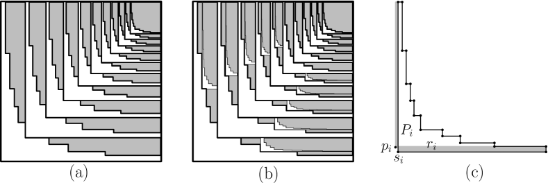
Figure 7: (a) An initial $\frac{2}{\varepsilon}$-staircase packing. (b) In any empty region (shaded gray), Alice can place an additional $\frac{2}{\varepsilon}$-staircase. (c) The placement of an extra point $p_{i}$ near the left side of the maximal rectangle $r_{i}\subset P_{i}$.

Alice first computes a packing of the unit square $U=[0,1]^{2}$ with $\frac{2}{\varepsilon}$-staircases, by successively choosing interior-disjoint $\frac{2}{\varepsilon}$-staircases of smaller and smaller sizes until their total area is at least $1-\frac{\varepsilon}{2}$ (Fig. 7(a,b)). Specifically, in the current step, given an axis aligned rectangle $R$ of height $h$ and width $w$, a $\frac{2}{\varepsilon}$ staircase polygon $P$ with the same height and width is anchored at the lower left corner of $R$, and the remaining space $R\setminus P$ is partitioned into vertical or horizontal sectors to be processed (see Section 3).

Then she slightly shrinks these staircases, to make them pairwise disjoint, and perturbs them to ensure that each $\frac{2}{\varepsilon}$-staircase $P_{i}$ contains a unique axis-aligned rectangle $r_{i}$ of maximum area, and $r_{i}$ has the same width as $P_{i}$. The point set $S$ contains, for every $\frac{2}{\varepsilon}$-staircase in this packing, all vertices of $P_{i}$, including the lower left corner $s_{i}$. In addition, for every $\frac{2}{\varepsilon}$-staircase whose lower left corner is not on the left side of $U$, $S$ also contains a point $p_{i}$ very close to the left side of rectangle $r_{i}$, as shown in Fig. 7(c).

It remains to determine the order in which Alice reveals the points to Bob. The points associated with each $\frac{2}{\varepsilon}$-staircase $P_{i}$ are revealed in a contiguous sequence such that the last two points in each sequence are the lower left corner $s_{i}$ followed by the extra point $p_{i}$. For the lower left corner $s_{i}$, Bob has to choose the unique rectangle $r_{i}$ of maximum area in $P_{i}$, which is adjacent to the lower side of $P_{i}$. For the extra point $p_{i}$, Bob has to choose a tall rectangle of negligible area, which covers the left side of $P_{i}$. These two rectangles guarantee that no subsequent rectangle can cover any additional part of $P_{i}$, while ${\rm area}(r_{i})\leq\frac{\varepsilon}{2}\cdot{\rm area}(P_{i})$.

To determine the order of sequences of points associated with the staircases, we define a partial order over the staircase polygons. Note that in the initial staircase packing, each tip of every $P_{i}$ is adjacent to the left or lower side of another staircase, or the right or upper side of $U$. This defines a partial order: let $P_{i}\prec P_{j}$, if the tip of $P_{j}$ is adjacent to the left or lower side of $P_{i}$; or if the lower left corner of $P_{i}$ is a reflex vertex of $P_{j}$. Order the staircases in any linear extension of this partial order. This ensures that Bob cannot choose a rectangle intersecting the interior of $P_{i}$ before Alice reveals the lower left corner $s_{i}$.

Best versus worst greedy strategy.

For a finite set $S\subset[0,1]^{2}$, and a permutation (ordering) $\pi$ of $S$, we can select anchored rectangles greedily (ties are broken arbitrarily) in the order prescribed by $\pi$. One can ask which permutation gives the best or the worst performance for a greedy strategy. Our main result, Theorem 3.13, says that for every $n$-element point set $S$, $(0,0)\in S$, we can find in $O(n\log n)$ time a permutation $\pi$ for which the greedy strategy covers $\Theta(1)$ area. In the worst case, greedy covers only $o(1)$ area by Theorem 4.1. In the best case, however, we will show (Lemma 4.3) that greedy is always optimal for some permutation $\pi$. We say that an anchored rectangle packing is Pareto optimal if each rectangle $r(s)$ has maximum area assuming that all other rectangles are fixed. It is clear that every optimal solution is Pareto optimal.

In particular, each rectangle in an optimal solution is bounded by the two rays (going up and to the right) from its anchor point, and two other such rays (from other points) that limit it from the right and from the top. This immediately implies the existence of an exact algorithm for the optimization problem running in exponential time, based on brute force enumeration. The next lemma also shows that the greedy algorithm and brute force enumeration of permutations yields yet another exact algorithm for the optimization problem.

Lemma 4.3

For every finite point set $S\subset[0,1]^{2}$ and every Pareto optimal anchored packing $R=\{r(s):s\in S\}$, there is a permutation $\pi$ for which a greedy algorithm (with some tie breaking) computes $R$.

Proof 4.4

Let $S\subset[0,1]^{2}$ be a finite set, which may not contain the origin. Since every $r(s)$ is Pareto optimal, it is a greedy choice assuming that $s$ is the last point in the order $\pi$. Suppose that $s\in S$ is the last point in a permutation $\pi$. If the smaller problem $S\setminus\{s\}$ with $R\setminus\{r(s)\}$ is not Pareto optimal, then there is a point $s^{\prime}\in S$ for which we could choose a larger rectangle anchored at $s^{\prime}$, which intersects $r(s)$ only. In this case, either $s$ dominates $s^{\prime}$ or the ray shot from $s^{\prime}$ vertically up (resp., horizontally right) hits the lower (resp., left) side of rectangle $r(s)$. This motivates the definition of a binary relation over $S$, which is an extension of the dominance order. Let $s^{\prime}\prec s$ if either $s$ dominates $s^{\prime}$ or an axis-aligned ray shot from $s^{\prime}$ hits the lower or left side of rectangle $r(s)$. It is not difficult to see that this is a partial order over $S$. If $s\in S$ is a minimal element in the poset $(S,\prec)$, then the rectangles in $R\setminus\{r(s)\}$ are still Pareto optimal for the anchors $S\setminus\{s\}$. Now let $\pi$ be the reverse order of any linear extension of this partial order.

We have shown (our main result) that for any set of $n$ points in the unit square $U=[0,1]^{2}$, one can find a set of disjoint empty rectangles anchored at the given points and covering more than $9\%$ of $U$. The same conclusion holds for points in any axis-aligned rectangle $V$ instead of $U$, since it is straightforward to use an affine transformation to map the input into the unit square. Concerning the bound obtained, a sizable gap to the conjectured $50\%$ remains. While certainly small adjustments in our proof can lead to improvements in the bound, obtaining substantial improvements probably requires new ideas.

Acknowledgement.

The authors thank Richard Guy for tracing back the origins of this problem and Jan Kynčl for comments and remarks.

References

-
[1]
Ponder this challenge: puzzle for June 2004;
http://domino.research.ibm.com/comm/wwwr_ponder.nsf/Challenges/June2004.html. - [2] M. Abramovitz and I. Stegun, Handbook of Mathematical Functions with Formulas, Graphs, and Mathematical Tables, Dover, New York, 1964.
- [3] N. Bansal, A. Caprara, and M. Sviridenko, A new approximation method for set covering problems, with applications to multidimensional bin packing, SIAM J. Comput. 39 (2009), 1256–1278.
- [4] N. Bansal, J. Correa, C. Kenyon, and M. Sviridenko, Bin packing in multiple dimensions: inapproximability results and approximation schemes, Math. Operat. Research 31 (2006), 31–49.
- [5] N. Bansal, X. Han, K. Iwama, M. Sviridenko, and G. Zhang, Harmonic algorithm for 3-dimensional strip packing problem, in Proc. 18th SODA, ACM-SIAM, 2007, pp. 1197–1206.
- [6] A. Caprara, Packing 2-dimensional bins in harmony, in Proc. 43rd FOCS, IEEE, 2002, pp. 490–499.
- [7] A. Caprara, Packing -dimensional bins in stages, Math. Oper. Res. 33 (2008), 203–215.
- [8] M. Chlebík and J. Chlebíková, Hardness of approximation for orthogonal rectangle packing and covering problems, J. Discrete Alg. 7 (3) (2009), 291–305.
- [9] T. Christ, A. Francke, H. Gebauer, J. Matoušek, and T. Uno, A doubly exponentially crumbled cake, manuscript, arXiv:1104.0122v1, 2011.
- [10] H. T. Croft, K. J. Falconer, and R. K. Guy, Unsolved Problems in Geometry, volume II of Unsolved Problems in Intuitive Mathematics, Springer, New York, 1991.
- [11] P. Erdős and R. L. Graham, Note on packing squares with equal squares, J. Combin. Theory Ser. A 19 (1975), 119–123.
- [12] R. Harren, K. Jansen, L. Prädel, and R. van Stee, A -approximation for strip packing, in Proc. 12th WADS, vol. 6844 of LNCS, Springer, 2011, to appear.
- [13] K. Jansen , L. Prädel, and U. M. Schwarz, Two for one: tight approximation of 2D bin packing, in Proc. 11th WADS, vol. 5664 of LNCS, Springer, 2009, pp. 399–410.
- [14] K. Jansen and R. Solis-Oba, A polynomial time approximation scheme for the square packing problem, in Proc. 13th IPCO, vol. 5035 of LNCS, Springer, 2008, pp. 184–198.
- [15] K. Jansen and G. Zhang, Maximizing the total profit of rectangles packed into a rectangle, Algorithmica 47 (3) (2007), 323–342.
- [16] L. Prädel, Approximation algorithms for two-dimensional geometrical knapsack, Masters thesis, Department of Computer Science, University of Kiel, 2008.
- [17] I. Schiermeyer, Reverse-fit: a 2-optimal algorithm for packing rectangles, in Proc. 2nd ESA, vol. 855 of LNCS, Springer, 1994, pp. 290–299.
- [18] A. Steinberg, A strip-packing algorithm with absolute performance bound 2, SIAM J. Comput. 26 (2) (1997), 401–409.
- [19] W. Tutte, Recent Progress in Combinatorics: Proceedings of the 3rd Waterloo Conference on Combinatorics, May 1968, Academic Press, New York, 1969.
- [20] P. Winkler, Packing rectangles, pp. 133-134, in Mathematical Mind-Benders, A. K. Peters Ltd., Wellesley, MA, 2007.
- [21] P. Winkler, Puzzled: rectangles galore, Communications of the ACM, 53 (11) (2010), 112.
- [22] P. Winkler, Puzzled: solutions and sources, Communications of the ACM, 53 (12) (2010), 128.