The Magic of Logical Inference in Probabilistic Programming

Abstract

Today, many different probabilistic programming languages exist and even more inference mechanisms for these languages. Still, most logic programming based languages use backward reasoning based on SLD resolution for inference. While these methods are typically computationally efficient, they often can neither handle infinite and/or continuous distributions, nor evidence. To overcome these limitations, we introduce distributional clauses, a variation and extension of Sato’s distribution semantics. We also contribute a novel approximate inference method that integrates forward reasoning with importance sampling, a well-known technique for probabilistic inference. To achieve efficiency, we integrate two logic programming techniques to direct forward sampling. Magic sets are used to focus on relevant parts of the program, while the integration of backward reasoning allows one to identify and avoid regions of the sample space that are inconsistent with the evidence.

1 Introduction

The advent of statistical relational learning [Getoor and Taskar (2007), De Raedt et al. (2008)] and probabilistic programming [De Raedt et al. (2008)] has resulted in a vast number of different languages and systems such as PRISM [Sato and Kameya (2001)], ICL [Poole (2008)], ProbLog [De Raedt et al. (2007)], Dyna [Eisner et al. (2005)], BLPs [Kersting and De Raedt (2008)], CLP($\mathcal{BN}$) [Santos Costa et al. (2008)], BLOG [Milch et al. (2005)], Church [Goodman et al. (2008)], IBAL [Pfeffer (2001)], and MLNs [Richardson and Domingos (2006)]. While inference in these languages generally involves evaluating the probability distribution defined by the model, often conditioned on evidence in the form of known truth values for some atoms, this diversity of systems has led to a variety of inference approaches. Languages such as IBAL, BLPs, MLNs and CLP($\mathcal{BN}$) combine knowledge-based model construction to generate a graphical model with standard inference techniques for such models. Some probabilistic programming languages, for instance BLOG and Church, use sampling for approximate inference in generative models, that is, they estimate probabilities from a large number of randomly generated program traces. Finally, probabilistic logic programming frameworks such as ICL, PRISM and ProbLog, combine SLD-resolution with probability calculations.

So far, the second approach based on sampling has received little attention in logic programming based systems. In this paper, we investigate the integration of sampling-based approaches into probabilistic logic programming frameworks to broaden the applicability of these. Particularly relevant in this regard are the ability of Church and BLOG to sample from continuous distributions and to answer conditional queries of the form $p(q|e)$ where $e$ is the evidence. To accommodate (continuous and discrete) distributions, we introduce distributional clauses, which define random variables together with their associated distributions, conditional upon logical predicates. Random variables can be passed around in the logic program and the outcome of a random variable can be compared with other values by means of special built-ins. To formally establish the semantics of this new construct, we show that these random variables define a basic distribution over facts (using the comparison built-ins) as required in Sato’s distribution semantics [Sato (1995)], and thus induces a distribution over least Herbrand models of the program. This contrasts with previous instances of the distribution semantics in that we no longer enumerate the probabilities of alternatives, but instead use arbitrary densities and distributions.

From a logic programming perspective, BLOG [Milch et al. (2005)] and related approaches perform forward reasoning, that is, the samples needed for probability estimation are generated starting from known facts and deriving additional facts, thus generating a possible world. PRISM and related approaches follow the opposite approach of backward reasoning, where inference starts from a query and follows a chain of rules backwards to the basic facts, thus generating proofs. This difference is one of the reasons for using sampling in the first approach: exact forward inference would require that all possible worlds be generated, which is infeasible in most cases. Based on this observation, we contribute a new inference method for probabilistic logic programming that combines sampling-based inference techniques with forward reasoning. On the probabilistic side, the approach uses rejection sampling [Koller and Friedman (2009)], a well-known sampling technique that rejects samples that are inconsistent with the evidence. On the logic programming side, we adapt the magic set technique [Bancilhon et al. (1986)] towards the probabilistic setting, thereby combining the advantages of forward and backward reasoning. Furthermore, the inference algorithm is improved along the lines of the SampleSearch algorithm [Gogate and Dechter (2011)], which avoids choices leading to a sample that cannot be used in the probability estimation due to inconsistency with the evidence. We realize this using a heuristic based on backward reasoning with limited proof length, the benefit of which is experimentally confirmed. This novel approach to inference creates a number of new possibilities for applications of probabilistic logic programming systems, including continuous distributions and Bayesian inference.

This paper is organized as follows: we start by reviewing the basic concepts in Section 2. Section 3 introduces the new language and its semantics, Section 4 a novel forward sampling algorithm for probabilistic logic programs. Before concluding, we evaluate our approach in Section 5.

2 Preliminaries

2.1 Probabilistic Inference

A discrete probabilistic model defines a probability distribution $p(\cdot)$ over a set $\Omega$ of basic outcomes, that is, value assignments to the model’s random variables. This distribution can then be used to evaluate a conditional probability distribution $p(q|e)=\frac{p(q\wedge e)}{p(e)}$, also called target distribution. Here, $q$ is a query involving random variables, and $e$ is the evidence, that is, a partial value assignment of the random variables. Evaluating this target distribution is called probabilistic inference [Koller and Friedman (2009)]. In probabilistic logic programming, random variables often correspond to ground atoms, and $p(\cdot)$ thus defines a distribution over truth value assignments, as we will see in more detail in Sec. 2.3 (but see also [De Raedt et al. (2008)]). Probabilistic inference then asks for the probability of a logical query being true given truth value assignments for a number of such ground atoms.

In general, the probability $p(\cdot)$ of a query $q$ is in the discrete case the sum over those outcomes $\omega\in\Omega$ that are consistent with the query. In the continuous case, the sum is replaced by an (multidimensional) integral and the distribution $p(\cdot)$ by a (product of) densities $\mathbf{F}(\cdot)$ That is,

$$p(q)=\sum_{\omega\in\Omega}p(\omega)\mymathbb{1}_{q}(\omega),\quad\quad and\quad\quad p(q)=\idotsint\limits_{\Omega}\mymathbb{1}_{q}(\omega)d\mathbf{F}(\omega)$$ (1)

where $\mymathbb{1}_{q}(\omega)=1$ if $\omega\models q$ and $0$ otherwise. As common (e.g. [Wasserman (2003)]) we will use for convenience the notation $\int xdF(x)$ as unifying notation for both discrete and continuous distributions.

As $\Omega$ is often very large or even infinite, exact inference based on the summation in (1) quickly becomes infeasible, and inference has to resort to approximation techniques based on samples, that is, randomly drawn outcomes $\omega\in\Omega$. Given a large set of such samples $\{s_{1},\ldots,s_{N}\}$ drawn from $p(\cdot)$, the probability $p(q)$ can be estimated as the fraction of samples where $q$ is true. If samples are instead drawn from the target distribution $p(\cdot|e)$, the latter can directly be estimated as

$$\hat{p}(q|e):=\frac{1}{N}\sum_{i=1}^{N}\mymathbb{1}_{q}(s_{i})\enspace.$$

However, sampling from $p(\cdot|e)$ is often highly inefficient or infeasible in practice, as the evidence needs to be taken into account. For instance, if one would use the standard definition of conditional probability to generate samples from $p(\cdot)$, all samples that are not consistent with the evidence do not contribute to the estimate and would thus have to be discarded or, in sampling terminology, rejected.

More advanced sampling methods therefore often resort to a so-called proposal distribution which allows for easier sampling. The error introduced by this simplification then needs to be accounted for when generating the estimate from the set of samples. An example for such a method is importance sampling, where each sample $s_{i}$ has an associated weight $w_{i}$. Samples are drawn from an importance distribution $\pi(\cdot|e)$, and weights are defined as $w_{i}=\frac{p(s_{i}|e)}{\pi(s_{i}|e)}$. The true target distribution can then be estimated as

$$\hat{p}(q|e)=\frac{1}{W}\sum_{i=1}^{N}w_{i}\cdot\mymathbb{1}_{q}(s_{i})$$

where $W=\sum_{i}w_{i}$ is a normalization constant. The simplest instance of this algorithm is rejection sampling as already sketched above, where the samples are drawn from the prior distribution $p(\cdot)$ and weights are $1$ for those samples consistent with the evidence, and $0$ for the others. Especially for evidence with low probability, rejection sampling suffers from a very high rejection rate, that is, many samples are generated, but do not contribute to the final estimate. This is known as the rejection problem. One way to address this problem is likelihood weighted sampling, which dynamically adapts the proposal distribution during sampling to avoid choosing values for random variables that cause the sample to become inconsistent with the evidence. Again, this requires corresponding modifications of the associated weights in order to produce correct estimates.

2.2 Logical Inference

A (definite) clause is an expression of the form $\mathtt{h\mbox{ :- }b_{1},\ldots,b_{n}}$, where $\mathtt{h}$ is called head and $\mathtt{b_{1},\ldots,b_{n}}$ is the body. A program consists of a set of clauses and its semantics is given by its least Herbrand model. There are at least two ways of using a definite clause in a logical derivation. First, there is backward chaining, which states that to prove a goal $\mathtt{h}$ with the clause it suffices to prove $\mathtt{b_{1},\ldots,b_{n}}$; second, there is forward chaining, which starts from a set of known facts $\mathtt{b_{1},\ldots,b_{n}}$ and the clause and concludes that $\mathtt{h}$ also holds (cf. [Nilsson and Małiszyński (1996)]). Prolog employs backward chaining (SLD-resolution) to answer queries. SLD-resolution is very efficient both in terms of time and space. However, similar subgoals may be derived multiple times if the query contains recursive calls. Moreover, SLD-resolution is not guaranteed to always terminate (when searching depth-first). Using forward reasoning, on the other hand, one starts with what is known and employs the immediate consequence operator $T_{P}$ until a fixpoint is reached. This fixpoint is identical to the least Herbrand model.

Definition 1 ($T_{P}$ operator).

Let $P$ be a logic program containing a set of definite clauses and $ground(P)$ the set of all ground instances of these clauses. Starting from a set of ground facts $S$ the $T_{P}$ operator returns

$$T_{P}(S)=\{\mathtt{h}\mid\mathtt{h\mbox{ :- }b_{1},\ldots,b_{n}}\in ground(P)\mbox{ and }\{\mathtt{b_{1}},\ldots,\mathtt{b_{n}}\}\subseteq S\}$$

2.3 Distribution Semantics

Sato’s distribution semantics [Sato (1995)] extends logic programming to the probabilistic setting by choosing truth values of basic facts randomly. The core of this semantics lies in splitting the logic program into a set $F$ of facts and a set $R$ of rules. Given a probability distribution $P_{F}$ over the facts, the rules then allow one to extend $P_{F}$ into a distribution over least Herbrand models of the logic program. Such a Herbrand model is called a possible world.

More precisely, it is assumed that $DB=F\cup R$ is ground and denumerable, and that no atom in $F$ unifies with the head of a rule in $R$. Each truth value assignment to $F$ gives rise to a unique least Herbrand model of $DB$. Thus, a probability distribution $P_{F}$ over $F$ can directly be extended into a distribution $P_{DB}$ over these models. Furthermore, Sato shows that, given an enumeration $f_{1},f_{2},\ldots$ of facts in $F$, $P_{F}$ can be constructed from a series of finite distributions $P_{F}^{(n)}(f_{1}=x_{1},\ldots,f_{n}=x_{n})$ provided that the series fulfills the so-called compatibility condition, that is,

$$P_{F}^{(n)}(f_{1}=x_{1},\ldots,f_{n}=x_{n})=\sum_{x_{n+1}}P_{F}^{(n+1)}(f_{1}=x_{1},\ldots,f_{n+1}=x_{n+1})$$ (2)

3 Syntax and Semantics

Sato’s distribution semantics, as summarized in Sec. 2.3, provides the basis for most probabilistic logic programming languages including PRISM [Sato and Kameya (2001)], ICL [Poole (2008)], CP-logic [Vennekens et al. (2009)] and ProbLog [De Raedt et al. (2007)]. The precise way of defining the basic distribution $P_{F}$ differs among languages, though the theoretical foundations are essentially the same. The most basic instance of the distribution semantics, employed by ProbLog, uses so-called probabilistic facts. Each ground instance of a probabilistic fact directly corresponds to an independent random variable that takes either the value “true” or “false”. These probabilistic facts can also be seen as binary switches, cf. [Sato (1995)], which again can be extended to multi-ary switches or choices as used by PRISM and ICL. For switches, at most one of the probabilistic facts belonging to the switch is “true” according to the specified distribution. Finally, in CP-logic, such choices are used in the head of rules leading to the so-called annotated disjunction.

Hybrid ProbLog [Gutmann et al. (2010)] extends the distribution semantics with continuous distributions. To allow for exact inference, Hybrid ProbLog imposes severe restrictions on the distributions and their further use in the program. Two sampled values, for instance, cannot be compared against each other. Only comparisons that involve one sampled value and one number constant are allowed. Sampled values may not be used in arithmetic expressions or as parameters for other distributions, for instance, it is not possible to sample a value and use it as the mean of a Gaussian distribution. It is also not possible to reason over an unknown number of objects as BLOG [Milch et al. (2005)] does, though this is the case mainly for algorithmic reasons.

Here, we alleviate these restrictions by defining the basic distribution $P_{F}$ over probabilistic facts based on both discrete and continuous random variables. We use a three-step approach to define this distribution. First, we introduce explicit random variables and corresponding distributions over their domains, both denoted by terms. Second, we use a mapping from these terms to terms denoting (sampled) outcomes, which, then, are used to define the basic distribution $P_{F}$ on the level of probabilistic facts. For instance, assume that an urn contains an unknown number of balls where the number is drawn from a Poisson distribution and we say that this urn contains many balls if it contains at least $10$ balls. We introduce a random variable $\mathtt{number}$, and we define $\mathtt{many}\mbox{ :- }\mathtt{dist\_gt(\simeq\!\!(number),9).}$ Here, $\simeq\!\!(\mathtt{number})$ is the Herbrand term denoting the sampled value of $\mathtt{number}$, and $\mathtt{dist\_gt(\simeq\!\!(number),9)}$ is a probabilistic fact whose probability of being true is the expectation that this value is actually greater than $9$. This probability then carries over to the derived atom $\mathtt{many}$ as well. We will elaborate on the details in the following.

3.1 Syntax

In a logic program, following Sato, we distinguish between probabilistic facts, which are used to define the basic distribution, and rules, which are used to derive additional atoms. Probabilistic facts are not allowed to unify with any rule head. The distribution over facts is based on random variables, whose distributions we define through so called distributional clauses.

Definition 2 (Distributional clause).

A distributional clause is a definite clause with an atom $\mathtt{h}\sim\mathcal{D}$ in the head where $\sim$ is a binary predicate used in infix notation.

For each ground instance $(\mathtt{h}\sim\mathcal{D}\mbox{ :- }\mathtt{b_{1},\ldots,b_{n}})\theta$ with $\theta$ being a substitution over the Herbrand universe of the logic program, the distributional clause defines a random variable $\mathtt{h}\theta$ and an associated distribution $\mathcal{D}\theta$. In fact, the distribution is only defined when $(\mathtt{b_{1},\ldots,b_{n}})\theta$ is true in the semantics of the logic program. These random variables are terms of the Herbrand universe and can be used as any other term in the logic program. Furthermore, a term $\simeq\!\!(d)$ constructed from the reserved functor $\simeq\!\!/1$ represents the outcome of the random variable $d$. These functors can be used inside calls to special predicates in $dist\_rel=\{dist\_eq/2,dist\_lt/2,dist\_leq/2,dist\_gt/2,dist\_geq/2\}$. We assume that there is a fact for each of the ground instances of these predicate calls. These facts are the probabilistic facts of Sato’s distribution semantics. Note that the set of probabilistic facts is enumerable as the Herbrand universe of the program is enumerable. A term $\simeq\!\!(d)$ links the random variable $d$ with its outcome. The probabilistic facts compare the outcome of a random variable with a constant or the outcome of another random variable and succeed or fail according to the probability distribution(s) of the random variable(s).

Example 1 (Distributional clauses).

$$\mathtt{nballs\sim poisson(6)}.$$ (3)

$$\mathtt{color(B)\sim\ [0.7:b,0.3:g]} \mbox{ :- }\mathtt{between(1,\simeq\!\!(nballs),B).}$$ (4)

$$\mathtt{diameter(B,MD)\sim gamma(MD/20,20)} \mathtt{\mbox{ :- }between(1,\simeq\!\!(nballs),B),}$$

$$\quad\ \mathtt{mean\_diameter(\simeq\!\!(color(B)),MD).}$$ (5)

The defined distributions depend on the following logical clauses:

$$\mathtt{mean\_diameter(C,5)} \mathtt{\mbox{ :- }dist\_eq(C,b).}$$

$$\mathtt{mean\_diameter(C,10)} \mathtt{\mbox{ :- }dist\_eq(C,g).}$$

$$\mathtt{between(I,J,I)} \mathtt{\mbox{ :- }dist\_leq(I,J).}$$

$$\mathtt{between(I,J,K)} \mathtt{\mbox{ :- }dist\_lt(I,J),\ I1\ is\ I+1,between(I1,J,K)}.$$

The distributional clause (3) models the number of balls as a Poisson distribution with mean 6. The distributional clause (4) models a discrete distribution for the random variable color(B). With probability 0.7 the ball is blue and green otherwise. Note that the distribution is defined only for the values B for which $between(1,\simeq\!\!(nballs),B)$ succeeds. Execution of calls to the latter give rise to calls to probabilistic facts that are instances of $dist\_leq(I,\simeq\!\!(nballs))$ and $dist\_lt(I,\simeq\!\!(nballs))$. Similarly, the distributional clause (5) defines a gamma distribution that is also conditionally defined. Note that the conditions in the distribution depend on calls of the form $mean\_diameter(\simeq\!\!(color(n)),MD)$ with $n$ a value returned by between/3. Execution of this call finally leads to calls $dist\_eq(\simeq\!\!(color(n)),b)$ and $dist\_eq(\simeq\!\!(color(n)),g)$.

It looks feasible, to allow $\simeq\!\!(d)$ terms everywhere and to have a simple program analysis insert the special predicates in the appropriate places by replacing $</2$, $>/2$, $\leq/2$, $\geq/2$ predicates by $dist\_rel/2$ facts. Though extending unification is a bit harder: as long as a $\simeq\!\!(h)$ term is unified with a free variable, standard unification can be performed; only when the other term is bound an extension is required. In this paper, we assume that the special predicates $\mathtt{dist\_eq/2}$, $\mathtt{dist\_lt/2}$, $\mathtt{dist\_leq/2}$, $\mathtt{dist\_gt/2}$, and $\mathtt{dist\_geq/2}$ are used whenever the outcome of a random variable need to be compared with another value and that it is safe to use standard unification whenever a $\mathtt{\simeq\!\!(h)}$ term is used in another predicate.

For the basic distribution on facts to be well-defined, a program has to fulfill a set of validity criteria that have to be enforced by the programmer.

Definition 3 (Valid program).

A program $P$ is called valid if:

(V1)

In the relation $\mathtt{h}\sim\mathcal{D}$ that holds in the least fixpoint of a program, there is a functional dependency from $\mathtt{h}$ to $\mathcal{D}$, so there is a unique ground distribution $\mathcal{D}$ for each ground random variable $\mathtt{h}$.

(V2)

The program is distribution-stratified, that is, there exists a function $rank(\cdot)$ that maps ground atoms to $\mathbb{N}$ and that satisfies the following properties: (1) for each ground instance of a distribution clause $\mathtt{h}\sim\mathcal{D}\mbox{ :- }\mathtt{b_{1},\ldots b_{n}}$ holds $rank(\mathtt{h}\sim\mathcal{D}>rank(\mathtt{b_{i}})$ (for all $i$). (2) for each ground instance of another program clause: $\mathtt{h}\mbox{ :- }\mathtt{b_{1},\ldots b_{n}}$ holds $rank(\mathtt{h})\geq rank(\mathtt{b_{i}})$ (for all $i$). (3) for each ground atom $\mathtt{b}$ that contains (the name of) a random variable $\mathtt{h}$, $rank(\mathtt{b})\geq rank(\mathtt{h}\sim\mathcal{D})$ (with $\mathtt{h}\sim\mathcal{D}$ the head of the distribution clause defining $\mathtt{h}$).

(V3)

All ground probabilistic facts or, to be more precise, the corresponding indicator functions are Lebesgue-measurable.

(V4)

Each atom in the least fixpoint can be derived from a finite number of probabilistic facts (finite support condition [Sato (1995)]).

Together, (V1) and (V2) ensure that a single basic distribution $P_{F}$ over the probabilistic facts can be obtained from the distributions of individual random variables defined in $P$. The requirement (V3) is crucial. It ensures that the series of distributions $P_{F}^{(n)}$ needed to construct this basic distribution is well-defined. Finally, the number of facts over which the basic distribution is defined needs to be countable. This is true, as we have a finite number of constants and functors: those appearing in the program.

3.2 Distribution Semantics

We now define the series of distributions $P_{F}^{(n)}$ where we fix an enumeration $f_{1},f_{2},\ldots$ of probabilistic facts such that $i<j\implies rank(f_{i})\leq rank(f_{j})$ where $rank(\cdot)$ is a ranking function showing that the program is distribution-stratified. For each predicate $\mathtt{rel/2}\in dist\_rel$, we define an indicator function as follows:

$$I^{1}_{rel}(X_{1},X_{2}) =\begin{cases}1&\text{if }\mathtt{rel}(X_{1},X_{2})\text{ is true}\\ 0&\text{if }\mathtt{rel}(X_{1},X_{2})\text{ is false}\end{cases}$$ (6)

Furthermore, we set $I^{0}_{rel}(X_{1},X_{2})=1.0-I^{1}_{rel}(X_{1},X_{2})$. We then use the expected value of the indicator function to define probability distributions $P_{F}^{(n)}$ over finite sets of ground facts $f_{1},\ldots,f_{n}$. Let $\{rv_{1},\ldots rv_{m}\}$ be the set of random variables these $n$ facts depend on, ordered such that if $rank(rv_{i})<rank(rv_{j})$, then $i<j$ (cf. (V2) in Definition 3). Furthermore, let $f_{i}=rel_{i}(t_{i1},t_{i2})$, $x_{j}\in\{1,0\}$, and $\theta^{-1}=\{\simeq\!\!(rv_{1})/V_{1},\ldots,\simeq\!\!(rv_{m})/V_{m}\}$. The latter replaces all evaluations of random variables on which the $f_{i}$ depend by variables for integration.

$$P_{F}^{(n)}(f_{1}=x_{1},\ldots,f_{n}=x_{n})=\mathbb{E}[I^{x_{1}}_{rel_{1}}(t_{11},t_{12}),\ldots,I^{x_{n}}_{rel_{n}}(t_{n1},t_{n2})]$$ (7)

$$=\idotsint\left(I^{x_{1}}_{rel_{1}}(t_{11}\theta^{-1},t_{12}\theta^{-1})\cdots I^{x_{n}}_{rel_{n}}(t_{n1}\theta^{-1},t_{n2})\theta^{-1}\right)d\mathcal{D}_{rv_{1}}(V_{1})\cdots d\mathcal{D}_{rv_{m}}(V_{m})$$

Example 2 (Basic Distribution).

Let $f_{1},f_{2},\ldots=dist\_lt(\simeq\!\!(b1),3),dist\_lt(\simeq\!\!(b2),\simeq\!\!(b1)),\ldots$. The second distribution in the series then is

$$P_{F}^{(2)}(dist\_lt(\simeq\!\!(b1),3)=x_{1},dist\_lt(\simeq\!\!(b2),\simeq\!\!(b1))=x_{2})$$

$$=\mathbb{E}[I_{\mathtt{dist\_lt}}^{x_{1}}(\simeq\!\!(b1),3),I_{\mathtt{dist\_lt}}^{x_{2}}(\simeq\!\!(b2),\simeq\!\!(b1))]$$

$$=\int\int\left(I_{\mathtt{dist\_lt}}^{x_{1}}(V1,3),I_{\mathtt{dist\_lt}}^{x_{2}}(V2,V1)\right)d\mathcal{D}_{b1}(V1)d\mathcal{D}_{b2}(V2)$$

By now we are able to prove the following proposition.

Proposition 1.

Let $P$ be a valid program. $P$ defines a probability measure $P_{P}$ over the set of fixpoints of the $T_{P}$ operator. Hence, $P$ also defines for an arbitrary formula $\mathtt{q}$ over atoms in its Herbrand base the probability that $\mathtt{q}$ is true.

Proof sketch.

It suffices to show that the series of distributions $P_{F}^{(n)}$ over facts (cf. (7)) is of the form that is required in the distribution semantics, that is, these are well-defined probability distributions that satisfy the compatibility condition, cf. (2). This is a direct consequence of the definition in terms of indicator functions and the measurability of the underlying facts required for valid programs. ∎

3.3 $T_{P}$ Semantics

In the following, we give a procedural view onto the semantics by extending the $T_{P}$ operator of Definition 1 to deal with probabilistic facts $\mathtt{dist\_rel(t_{1},t_{2})}$. To do so, we introduce a function ReadTable$(\cdot)$ that keeps track of the sampled values of random variables to evaluate probabilistic facts. This is required because interpretations of a program only contain such probabilistic facts, but not the underlying outcomes of random variables. Given a probabilistic fact $\mathtt{dist\_rel(t1,t2)}$, ReadTable returns the truth value of the fact based on the values of the random variables $h$ in the arguments, which are either retrieved from the table or sampled according to their definition $\mathtt{h}\sim\mathcal{D}$ as included in the interpretation and stored in case they are not yet available.

Definition 4 (Stochastic $T_{P}$ operator).

Let $P$ be a valid program and $ground(P)$ the set of all ground instances of clauses in $P$. Starting from a set of ground facts $S$ the $ST_{P}$ operator returns

$$ST_{P}(S):=\Big{\{}\mathtt{h}\ \Big{|}\ \mathtt{h\mbox{ :- }b_{1},\ldots,b_{n}}\in ground(P)\mbox{ and }\forall\ \mathtt{b_{i}}:\mbox{ either }\mathtt{b_{i}}\in S\mbox{ or }$$

$$\big{(}\mathtt{b_{i}}=dist\_rel(t1,t2)\wedge(t_{j}=\simeq\!\!(h)\rightarrow(\mathtt{h}\sim\mathcal{D})\in S)\wedge$$

$$\ \mbox{{ReadTable}}(b_{i})=true\big{)}\Big{\}}$$

ReadTable ensures that the basic facts are sampled from their joint distribution as defined in Sec. 3.2 during the construction of the standard fixpoint of the logic program. Thus, each fixpoint of the $ST_{P}$ operator corresponds to a possible world whose probability is given by the distribution semantics.

4 Forward sampling using Magic Sets and backward reasoning

In this section we introduce our new method for probabilistic forward inference. To this aim, we first extend the magic set transformation to distributional clauses. We then develop a rejection sampling scheme using this transformation. This scheme also incorporates backward reasoning to check for consistency with the evidence during sampling and thus to reduce the rejection rate.

4.1 Probabilistic magic set transformation

The disadvantage of forward reasoning in logic programming is that the search is not goal-driven, which might generate irrelevant atoms. The magic set transformation [Bancilhon et al. (1986), Nilsson and Małiszyński (1996)] focuses forward reasoning in logic programs towards a goal to avoid the generation of uninteresting facts. It thus combines the advantages of both reasoning directions.

Definition 5 (Magic Set Transformation).

If $P$ is a logic program, then we use $\textsc{Magic}(P)$ to denote the smallest program such that if $\mathtt{A_{0}\mbox{ :- }A_{1},\ldots,A_{n}}\in P$ then

• $\mathtt{A_{0}\mbox{ :- }c(A_{0}),A_{1},\ldots,A_{n}}\in\textsc{Magic}(P)$ and

• for each $1\leq i\leq n$: $\mathtt{c(A_{i})\mbox{ :- }c(A_{0}),A_{1},\ldots,A_{i-1}}\in\textsc{Magic}(P)$

The meaning of the additional $\mathtt{c/1}$ atoms (c=call) is that they “switch on” clauses when they are needed to prove a particular goal. If the corresponding switch for the head atom is not true, the body is not true and thus cannot be proven. The magic transformation is both sound and complete. Furthermore, if the SLD-tree of a goal is finite, forward reasoning in the transformed program terminates. The same holds if forward reasoning on the original program terminates.

We now extend this transformation to distributional clauses. The idea is that the distributional clause for a random variable $h$ is activated when there is a call to a probabilistic fact $dist\_rel(t_{1},t_{2})$ depending on $h$.

Definition 6 (Probabilistic Magic Set Transformation).

For program $P$, let $P_{L}$ be $P$ without distributional clauses. $\textsc{M}(P)$ is the smallest program s.t. $\textsc{Magic}(P_{L})\subseteq\textsc{M}(P)$ and for each $\mathtt{h}\sim\mathcal{D}\mathtt{\mbox{ :- }b_{1},\ldots,b_{n}}\in P$ and $\mathtt{rel}\in\{\mathtt{eq,lt,leq,gt,geq}\}$:

• $\mathtt{h}\sim\mathcal{D}\mbox{ :- }\mathtt{(c(dist\_rel(\simeq\!\!(h),X));c(dist\_rel(X,\simeq\!\!(h))),b_{1},\ldots,b_{n}.}\in\textsc{M}(P)$.

• $\mathtt{c(b_{i})\mbox{ :- }(c(dist\_rel(\simeq\!\!(h),X));c(dist\_rel(X,\simeq\!\!(h))),b_{1},\ldots,b_{i-1}.}\in\textsc{M}(P)$.

Then $\textsc{PMagic}(P)$ consists of:

• a clause $\mathtt{a\_p(t_{1},\ldots,t_{n})}\mbox{ :- }\mathtt{c(p(t_{1},\ldots,t_{n})),p(t_{1},\ldots,t_{n})}$ for each built-in predicate (including $\mathtt{dist\_rel/2}$ for $\mathtt{rel}\in\{\mathtt{eq,lt,leq,gt,geq}\}$) used in $\textsc{M}(P)$.

• a clause $\mathtt{h}\mbox{ :- }\mathtt{b_{1}^{\prime},\ldots,b_{n}^{\prime}}$ for each clause $\mathtt{h}\mbox{ :- }\mathtt{b_{1},\ldots,b_{n}}\in\textsc{M}(P)$ where $\mathtt{b_{i}^{\prime}=a\_b_{i}}$ if $\mathtt{b_{i}}$ uses a built-in predicate and else $\mathtt{b_{i}^{\prime}=b_{i}}$.

Note that every call to a built-in $\mathtt{b}$ is replaced by a call to $\mathtt{a\_b}$; the latter predicate is defined by a clause that is activated when there is a call to the built-in ($\mathtt{c(b)}$) and that effectively calls the built-in. The transformed program computes the distributions only for random variables whose value is relevant to the query. These distributions are the same as those obtained in a forward computation of the original program. Hence we can show:

Lemma 1.

Let $P$ be a program and $\textsc{PMagic}(P)$ its probabilistic magic set transformation extended with a seed $c(q)$. The distribution over $q$ defined by $P$ and by $\textsc{PMagic}(P)$ is the same.

Proof sketch.

In both programs, the distribution over $q$ is determined by the distributions of the atoms $dist\_eq(t_{1},t_{2})$, $dist\_leq(t_{1},t_{2})$, $dist\_lt(t_{1},t_{2})$, $dist\_geq(t_{1},t_{2})$, and $dist\_gt(t_{1},t_{2})$ on which $q$ depends in a forward computation of the program $P$. The magic set transformation ensures that these atoms are called in the forward execution of $\textsc{PMagic}(P)$. In $\textsc{PMagic}(P)$, a call to such an atom activates the distributional clause for the involved random variable. As this distributional clause is a logic program clause, soundness and completeness of the magic set transformation ensures that the distribution obtained for that random variable is the same as in $P$. Hence also the distribution over $q$ is the same for both programs. ∎

4.2 Rejection sampling with heuristic lookahead

As discussed in Section 2.1, sampling-based approaches to probabilistic inference estimate the conditional probability $p(q|e)$ of a query $q$ given evidence $e$ by randomly generating a large number of samples or possible worlds (cf. Algorithm 1). The algorithm starts by preparing the program $L$ for sampling by applying the PMagic transformation. In the following, we discuss our choice of subroutine STPMagic (cf. Algorithm 2) which realizes likelihood weighted sampling. It is used in Algorithm 1, line 5, to generate individual samples. It iterates the stochastic consequence operator of Definition 4 until either a fixpoint is reached or the current sample is inconsistent with the evidence. Finally, if the sample is inconsistent with the evidence, it receives weight 0.

Algorithm 1 Main loop for sampling-based inference to calculate the conditional probability $p(q|e)$ for query $q$, evidence $e$ and program $L$.

1:function Evaluate($L$, $q$, $e$, $Depth$)

2:     $L^{*}:=$PMagic$(L)\cup\{c(a)|a\in e\cup{q}\}$

3:     $n^{+}:=0$           $n^{-}:=0$

4:     while Not converged do

5:         $(I,w):=$STPMagic$(L^{*},L,e,Depth)$

6:         if $q\in I$ then $n^{+}:=n^{+}+w$ else $n^{-}:=n^{-}+w$      

7:     return $n^{+}/(n^{+}+n^{-})$

Algorithm 2 Sampling one interpretation; used in Algorithm 1.

1:function STPMagic($L^{*},L,e,Depth$)

2:     $T_{pf}:=\varnothing$, $T_{dis}:=\varnothing$, $w:=1$, $I_{old}:=\varnothing$, $I_{new}:=\varnothing$

3:     repeat

4:         $I_{old}:=I_{new}$

5:         for all $(\mathtt{h\mbox{ :- }\ body)}\ \in L^{*}$ do

6:              split body in $B_{PF}$ (prob. facts) and $B_{L}$ (the rest)

7:              for all grounding substitution $\theta$ such that $B_{L}\theta\subseteq I_{old}$ do

8:                  $s:=true$, $w_{d}:=1$

9:                  while $s\wedge B_{PF}\neq\varnothing$ do

10:                       select and remove $pf$ from $B_{PF}$

11:                       $(b_{pf},w_{pf}):=$ReadTable$(pf\theta,I_{old},T_{pf},T_{dis},L,e,Depth)$

12:                       $s:=s\wedge b_{pf}$           $w_{d}:=w_{d}\cdot w_{pf}$                   

13:                  if $s$ then

14:                       if $h\theta\in e^{-}$ then return $(I_{new},0)$ $\triangleright$ check negative evidence                        

15:                       $I_{new}:=I_{new}\cup\{h\theta\}$           $w:=w\cdot w_{d}$                                          

16:     until $I_{new}=I_{old}\vee w=0$ $\triangleright$ Fixpoint or impossible evidence

17:     if $e^{+}\subseteq I_{new}$ then return $(I_{new},w)$ $\triangleright$ check positive evidence

18:     else return $(I_{new},0)$     

Algorithm 3 Evaluating a probabilistic fact $pf$; used in Algorithm 2. ComputePF$(pf,T_{dis})$ computes the truth value and the probability of $pf$ according to the information in $T_{dis}$.

1:function ReadTable($pf,I,T_{pf},T_{dis},L,e,Depth$)

2:     if $pf\notin T_{pf}$ then

3:         for all random variable $h$ occurring in $pf$ where $h\notin T_{dis}$ do

4:              if $h\sim D\notin I$ then return $(false,0)$               

5:              if not Sample($h,D,T_{dis},I,L,e,Depth$) then return $(false,0)$                        

6:         $(b,w):=$ ComputePF($pf$,$T_{dis}$)

7:         if $(b\wedge(pf\in e^{-}))\vee(\neg b\wedge(pf\in e^{+}))$ then

8:              return $(false,0)$ $\triangleright$ inconsistent with evidence         

9:         extend $T_{pf}$ with $(pf,b,w)$      

10:     return $(b,w)$ as stored in $T_{pf}$ for $pf$

11:procedure Sample($\mathtt{h},\mathcal{D},\ T_{dis},\ I,\ L,\ e,\ Depth$)

12:     $w_{h}:=1$, $\mathcal{D}^{\prime}:=\mathcal{D}$ $\triangleright$ Initial weight, temp. distribution

13:     if $\mathcal{D}^{\prime}=[p_{1}:\mathtt{a_{1}},\ldots,p_{n}:\mathtt{a_{n}}]$ then $\triangleright$ finite distribution

14:         for $p_{j}:\mathtt{a_{j}}\in\mathcal{D}^{\prime}$ where $\mathtt{dist\_eq}(\mathtt{h},\mathtt{a_{j}})\in e^{-}$ do $\triangleright$ remove neg. evidence

15:              $\mathcal{D}^{\prime}:=\textsc{Norm}(\mathcal{D}^{\prime}\setminus\{p_{j}:\mathtt{a_{j}}\})$,          $w_{h}:=w_{h}\times(1-p_{j})$          

16:         if $\exists v:\mathtt{dist\_eq(\simeq\!\!(h),v)}\in e^{+}$ and $p:\mathtt{v}\in\mathcal{D}^{\prime}$ then

17:              $\mathcal{D}^{\prime}:=[1:v]$,           $w_{h}:=w_{h}\times p$          

18:         for $p_{j}:\mathtt{a_{j}}\in\mathcal{D}^{\prime}$ do $\triangleright$ remove choices that make $e^{+}$ impossible

19:              if $\exists b\in e^{+}$: not MaybeProof($b,Depth,I\cup\{\mathtt{dist\_eq}(\mathtt{h},\mathtt{a_{j}})\},L$) or

20:                 $\exists b\in e^{-}$: not MaybeFail($b,Depth,I\cup\{\mathtt{dist\_eq}(\mathtt{h},\mathtt{a_{j}})\},L$)  then

21:                  $\mathcal{D}^{\prime}:=\textsc{Norm}(\mathcal{D}^{\prime}\setminus\{p_{j}:\mathtt{a_{j}}\})$,          $w_{h}:=w_{h}\times(1-p_{j})$                             

22:     if $\mathcal{D}^{\prime}=\varnothing$ return false

23:     Sample $x$ according to $\mathcal{D^{\prime}}$, extend $T_{dis}$ with $(h,x)$ and return true

Algorithm 3 details the procedure used in line 11 of Algorithm 2 to sample from a given distributional clause. The function ReadTable returns the truth value of the probabilistic fact, together with its weight. If the outcome is not yet tabled, it is computed. Note that false is returned when the outcome is not consistent with the evidence. Involved distributions, if not yet tabled, are sampled in line 5. In the infinite case, Sample simply returns the sampled value. In the finite case, it is directed towards generating samples that are consistent with the evidence. Firstly, all possible choices that are inconsistent with the negative evidence are removed. Secondly, when there is positive evidence for a particular value, only that value is left in the distribution. Thirdly, it is checked whether each left value is consistent with all other evidence. This consistency check is performed by a simple depth-bounded meta-interpreter. For positive evidence, it attempts a top-down proof of the evidence atom in the original program using the function MaybeProof. Subgoals for which the depth-bound is reached, as well as probabilistic facts that are not yet tabled are assumed to succeed. If this results in a proof, the value is consistent, otherwise it is removed. Similarly for negative evidence: in MaybeFail, subgoals for which the depth-bound is reached, as well as probabilistic facts that are not yet tabled are assumed to fail. If this results in failure, the value is consistent, otherwise it is removed. The $Depth$ parameter allows one to trade the computational cost associated with this consistency check for a reduced rejection rate.

Note that the modified distribution is normalized and the weight is adjusted in each of these three cases. The weight adjustment takes into account that removed elements cannot be sampled and is necessary as it can depend on the distributions sampled so far which elements are removed from the distribution sampled in Sample (the clause bodies of the distribution clause are instantiating the distribution).

5 Experiments

We implemented our algorithm in YAP Prolog and set up experiments to answer the questions

• Does the lookahead-based sampling improve the performance?

• How do rejection sampling and likelihood weighting compare?

To answer the first question, we used the distributional program in Figure 1, which models an urn containing a random number of balls. The number of balls is uniformly distributed between 1 and 10 and each ball is either red or green with equal probability. We draw 8 times a ball with replacement from the urn and observe its color. We also define the atom $\mathtt{nogreen(}D\mathtt{)}$ to be true if and only if we did not draw any green ball in draw 1 to $D$. We evaluated the query $P(\mathtt{dist\_eq(\simeq(color(\simeq(drawnball(1)))),red)}\ |\mathtt{nogreen(}D\mathtt{)})$ for $D=1,2,\ldots,8$. Note that the evidence implies that the first drawn ball is red, hence that the probability of the query is 1; however, the number of steps required to proof that the evidence is inconsistent with drawing a green first ball increases with D, so the larger is D, the larger Depth is required to reach a 100% acceptance rate for the sample as illustrated in Figure  1. It is clear that by increasing the depth limit, each sample will take longer to be generated. Thus, the $Depth$ parameter allows one to trade off convergence speed of the sampling and the time each sample needs to be generated. Depending on the program, the query, and the evidence there is an optimal depth for the lookahead.

$$\mathtt{numballs\sim uniform([1,2,3,4,5,6,7,8,9,10]).}$$

$$\mathtt{ball(M)\mbox{ :- }between(1,numballs,M).}$$

$$\mathtt{color(B)\sim uniform([red,green])\mbox{ :- }ball(B).}$$

$$\mathtt{draw(N)\mbox{ :- }between(1,8,N).}$$

$$\mathtt{nogreen(0).}$$

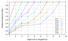
$$\mathtt{nogreen(D)\mbox{ :- }dist\_eq(\simeq(color(\simeq(drawnball(D)))),red),\ D2\ is\ D-1,\ nogreen(D2).}$$

$$\mathtt{drawnball(D)\sim uniform(L)\mbox{ :- }draw(D),}\mathtt{findall(B,ball(B),L).}$$

Figure 1: The program modeling the urn (left); rate of accepted samples (right) for evaluating the query $P(\mathtt{dist\_eq(\simeq(color(\simeq(drawnball(1)))),red)}\ |$ $\mathtt{nogreen(}D\mathtt{)})$ for $D=1,2,\ldots,10$ and for $Depth=1,2,\ldots,8$ using Algorithm 1. The acceptance rate is calculated by generating 200 samples using our algorithm and counting the number of sample with weight larger than 0.

To answer Q2, we used the standard example for BLOG [Milch et al. (2005)]. An urn contains an unknown number of balls where every ball can be either green or blue with $p=0.5$. When drawing a ball from the urn, we observe its color but do not know which ball it is. When we observe the color of a particular ball, there is a $20\%$ chance to observe the wrong one, e.g. green instead of blue. We have some prior belief over the number of balls in the urn. If 10 balls are drawn with replacement from the urn and we saw 10 times the color green, what is the probability that there are $n$ balls in the urn? We consider two different prior distributions: in the first case, the number of balls is uniformly distributed between 1 and 8, in the second case, it is Poisson-distributed with mean $\lambda=6$.

Figure 2: Results of urn experiment with forward reasoning. 10 balls with replacement were drawn and each time green was observed. Left: Uniform prior over # balls, right: Poisson prior $(\lambda=6)$.

One run of the experiment corresponds to sampling the number $N$ of balls in the urn, the color for each of the $N$ balls, and for each of the ten draws both the ball drawn and whether or not the color is observed correctly in this draw. Once these values are fixed, the sequence of colors observed is determined. This implies that for a fixed number $N$ of balls, there are $2^{N}\cdot N^{10}$ possible proofs. In case of the uniform distribution, exact PRISM inference can be used to calculate the probability for each given number of balls, with a total runtime of $0.16$ seconds for all eight cases. In the case of the Poisson distribution, this is only possible up to 13 balls, with more balls, PRISM runs out of memory. For inference using sampling, we generate 20,000 samples with the uniform prior, and 100,000 with Poisson prior. We report average results over five repetitions. For these priors, PRISM generates 8,015 and 7,507 samples per second respectively, ProbLog backward sampling 708 and 510, BLOG 3,008 and 2,900, and our new forward sampling (with rejection sampling) 760 and 731. The results using our algorithm for both rejection sampling and likelihood weighting with $Depth=0$ are shown in Figure 2. As the graphs show, the standard deviation for rejection sampling is much larger than for likelihood weighting.

6 Conclusions and related work

We have contributed a novel construct for probabilistic logic programming, the distributional clauses, and defined its semantics. Distributional clauses allow one to represent continuous variables and to reason about an unknown number of objects. In this regard this construct is similar in spirit to languages such as BLOG and Church, but it is strongly embedded in a logic programming context. This embedding allowed us to propose also a novel inference method based on a combination of importance sampling and forward reasoning. This contrasts with the majority of probabilistic logic programming languages which are based on backward reasoning (possibly enhanced with tabling [Sato and Kameya (2001), Mantadelis and Janssens (2010)]). Furthermore, only few of these techniques employ sampling, but see [Kimmig et al. (2011)] for a Monte Carlo approach using backward reasoning. Another key difference with the existing probabilistic logic programming approaches is that the described inference method can handle evidence. This is due to the magic set transformation that targets the generative process towards the query and evidence and instantiates only relevant random variables.

P-log [Baral et al. (2009)] is a probabilistic language based on Answer Set Prolog (ASP). It uses a standard ASP solver for inference and thus is based on forward reasoning, but without the use of sampling. Magic sets are also used in probabilistic Datalog [Fuhr (2000)], as well as in Dyna, a probabilistic logic programming language [Eisner et al. (2005)] based on rewrite rules that uses forward reasoning. However, neither of them uses sampling. Furthermore, Dyna and PRISM require that the exclusive-explanation assumption. This assumption states that no two different proofs for the same goal can be true simultaneously, that is, they have to rely on at least one basic random variable with different outcome. Distributional clauses (and the ProbLog language) do not impose such a restriction. Other related work includes MCMC-based sampling algorithms such as the approach for SLP [Angelopoulos and Cussens (2003)]. Church’s inference algorithm is based on MCMC too, and also BLOG is able to employ MCMC. At least for BLOG it seems to be required to define a domain-specific proposal distribution for fast convergence. With regard to future work, it would be interesting to consider evidence on continuous distributions as it is currently restricted to finite distribution. Program analysis and transformation techniques to further optimize the program w.r.t. the evidence and query could be used to increase the sampling speed. Finally, the implementation could be optimized by memoizing some information from previous runs and then use it to more rapidly prune as well as sample.

References

- Angelopoulos and Cussens (2003) Angelopoulos, N. and Cussens, J. 2003. Prolog issues and experimental results of an MCMC algorithm. In Web Knowledge Management and Decision Support, O. Bartenstein, U. Geske, M. Hannebauer, and O. Yoshie, Eds. Lecture Notes in Computer Science, vol. 2543. Springer, Berlin / Heidelberg, 186–196.
- Bancilhon et al. (1986) Bancilhon, F., Maier, D., Sagiv, Y., and Jeffrey D. Ullman. 1986. Magic sets and other strange ways to implement logic programs (extended abstract). In Proceedings of the fifth ACM SIGACT-SIGMOD symposium on Principles of database systems (PODS 1986). ACM, Cambridge, Massachusetts, United States, 1–15.
- Baral et al. (2009) Baral, C., Gelfond, M., and Rushton, N. 2009. Probabilistic reasoning with answer sets. Theory and Practice of Logic Programming 9, 1, 57–144.
- De Raedt et al. (2008) De Raedt, L., Demoen, B., Fierens, D., Gutmann, B., Janssens, G., Kimmig, A., Landwehr, N., Mantadelis, T., Meert, W., Rocha, R., Santos Costa, V., Thon, I., and Vennekens, J. 2008. Towards digesting the alphabet-soup of statistical relational learning. In Proceedings of the 1st Workshop on Probabilistic Programming: Universal Languages, Systems and Applications, D. Roy, J. Winn, D. McAllester, V. Mansinghka, and J. Tenenbaum, Eds. Whistler, Canada.
- De Raedt et al. (2008) De Raedt, L., Frasconi, P., Kersting, K., and Muggleton, S. 2008. Probabilistic Inductive Logic Programming - Theory and Applications. LNCS, vol. 4911. Springer, Berlin / Heidelberg.
- De Raedt et al. (2007) De Raedt, L., Kimmig, A., and Toivonen, H. 2007. ProbLog: A probabilistic Prolog and its application in link discovery. In IJCAI. 2462–2467.
- Eisner et al. (2005) Eisner, J., Goldlust, E., and Smith, N. 2005. Compiling Comp Ling: Weighted dynamic programming and the Dyna language. In Proceedings of the Human Language Technology Conference and Conference on Empirical Methods in Natural Language Processing (HLT/EMNLP-05).
- Fuhr (2000) Fuhr, N. 2000. Probabilistic Datalog: Implementing logical information retrieval for advanced applications. Journal of the American Society for Information Science (JASIS) 51, 2, 95–110.
- Getoor and Taskar (2007) Getoor, L. and Taskar, B. 2007. An Introduction to Statistical Relational Learning. MIT Press.
- Gogate and Dechter (2011) Gogate, V. and Dechter, R. 2011. SampleSearch: Importance sampling in presence of determinism. Artif. Intell. 175, 694–729.
- Goodman et al. (2008) Goodman, N., Mansinghka, V. K., Roy, D. M., Bonawitz, K., and Tenenbaum, J. B. 2008. Church: A language for generative models. In UAI. 220–229.
- Gutmann et al. (2010) Gutmann, B., Jaeger, M., and De Raedt, L. 2010. Extending ProbLog with continuous distributions. In Proceedings of the 20th International Conference on Inductive Logic Programming (ILP–10), P. Frasconi and F. A. Lisi, Eds. Firenze, Italy.
- Kersting and De Raedt (2008) Kersting, K. and De Raedt, L. 2008. Basic principles of learning Bayesian logic programs. See De Raedt et al. (2008), 189–221.
- Kimmig et al. (2011) Kimmig, A., Demoen, B., De Raedt, L., Santos Costa, V., and Rocha, R. 2011. On the implementation of the probabilistic logic programming language ProbLog. Theory and Practice of Logic Programming (TPLP) 11, 235–262.
- Koller and Friedman (2009) Koller, D. and Friedman, N. 2009. Probabilistic Graphical Models: Principles and Techniques. MIT Press.
- Mantadelis and Janssens (2010) Mantadelis, T. and Janssens, G. 2010. Dedicated tabling for a probabilistic setting. In Technical Communications of the 26th International Conference on Logic Programming (ICLP-10), M. V. Hermenegildo and T. Schaub, Eds. LIPIcs, vol. 7. Schloss Dagstuhl - Leibniz-Zentrum für Informatik, 124–133.
- Milch et al. (2005) Milch, B., Marthi, B., Russell, S., Sontag, D., Ong, D., and Kolobov, A. 2005. BLOG: Probabilistic models with unknown objects. In IJCAI. 1352–1359.
- Milch et al. (2005) Milch, B., Marthi, B., Sontag, D., Russell, S., Ong, D. L., and Kolobov, A. 2005. Approximate inference for infinite contingent Bayesian networks. In Proceedings of the Tenth International Workshop on Artificial Intelligence and Statistics, Jan 6-8, 2005, Savannah Hotel, Barbados, R. G. Cowell and Z. Ghahramani, Eds. Society for Artificial Intelligence and Statistics, 238–245. (Available electronically at http://www.gatsby.ucl.ac.uk/aistats/).
- Nilsson and Małiszyński (1996) Nilsson, U. and Małiszyński, J. 1996. Logic, Programming And Prolog, 2nd ed. Wiley & Sons.
- Pfeffer (2001) Pfeffer, A. 2001. IBAL: A probabilistic rational programming language. In IJCAI. 733–740.
- Poole (2008) Poole, D. 2008. The independent choice logic and beyond. In Probabilistic Inductive Logic Programming - Theory and Applications, L. De Raedt, P. Frasconi, K. Kersting, and S. Muggleton, Eds. LNCS, vol. 4911. Springer, Berlin/Heidelberg, 222–243.
- Richardson and Domingos (2006) Richardson, M. and Domingos, P. 2006. Markov logic networks. Machine Learning 62, 1-2, 107–136.
- Santos Costa et al. (2008) Santos Costa, V., Page, D., and Cussens, J. 2008. CLP(BN): Constraint logic programming for probabilistic knowledge. See De Raedt et al. (2008), 156–188.
- Sato (1995) Sato, T. 1995. A statistical learning method for logic programs with distribution semantics. In Proceedings of the Twelth International Conference on Logic Programming (ICLP 1995). MIT Press, 715–729.
- Sato and Kameya (2001) Sato, T. and Kameya, Y. 2001. Parameter learning of logic programs for symbolic-statistical modeling. Journal of Artificial Intelligence Resesearch (JAIR) 15, 391–454.
- Vennekens et al. (2009) Vennekens, J., Denecker, M., and Bruynooghe, M. 2009. CP-logic: A language of causal probabilistic events and its relation to logic programming. Theory and Practice of Logic Programming 9, 3, 245–308.
- Wasserman (2003) Wasserman, L. 2003. All of Statistics: A Concise Course in Statistical Inference (Springer Texts in Statistics). Springer.