The metallicity distribution of bulge clump giants in Baade’s Window ^,

Abstract

Aims. We seek to constrain the formation of the Galactic bulge by means of analysing the detailed chemical composition of a large sample of red clump stars in Baade’s window.

Methods. We measure [Fe/H] in a sample of 219 bulge red clump stars from R=20000 resolution spectra obtained with FLAMES/GIRAFFE at the VLT, using an automatic procedure, differentially to the metal-rich local reference star $\mu$Leo. For a subsample of 162 stars, we also derive [Mg/H] from spectral synthesis around the Mg I triplet at $\rm\lambda$ 6319 Å.

Results. The Fe and Mg metallicity distributions are both asymmetric, with median values of $+0.16$ and $+0.21$ respectively. The iron distribution is clearly bimodal, as revealed both by a deconvolution (from observational errors) and a Gaussian decomposition. The decomposition of the observed Fe and Mg metallicity distributions into Gaussian components yields two populations of equal sizes (50% each): a metal-poor component centred around [Fe/H] $\rm=-0.30$ and [Mg/H] $\rm=-0.06$ with a large dispersion and a narrow metal-rich component centred around $\rm[Fe/H]=+0.32$ and $\rm[Mg/H]=+0.35$. The metal poor component shows high [Mg/Fe] ratios (around 0.3) whereas stars in the metal rich component are found to have near solar ratios. Babusiaux et al. (2010) also find kinematical differences between the two components: the metal poor component shows kinematics compatible with an old spheroid whereas the metal rich component is consistent with a population supporting a bar. In view of their chemical and kinematical properties, we suggest different formation scenarii for the two populations: a rapid formation timescale as an old spheroid for the metal poor component (old bulge) and for the metal rich component, a formation over a longer time scale driven by the evolution of the bar (pseudo-bulge).

Conclusions. Guided by these results, we build a simple model combining two components: a simple closed box model to predict the metal poor population contribution, whereas the metal rich population is modelled using the observed local thin disc metallicity distribution, shifted in metallicity. The pseudo-bulge is compatible with being formed from the inner thin disc, assuming large (but plausible) values of the gradients in the early Galactic disc.

1 Introduction

The Milky-Way bulge has been the subject of quite intense debates in the community, as its status is not yet fully established. With various stellar population characteristics similar to those of the central old spheroids found at the centre of earlier-type galaxies, and others (mostly geometrical and kinematical) that rather point towards a very strong influence of a bar responsible for a pseudo-bulge, it sits at the border between these two types of bulges. The formation scenarios for bulges can be classified in three different types: (i) initial collapse of gas at early times (see e.g. Eggen et al., 1962); (ii) merging subclumps, either through an early disc evolution (Noguchi, 1999; Immeli et al., 2004), or through mergers (Aguerri et al., 2001; Scannapieco & Tissera, 2003; Nakasato & Nomoto, 2003); (iii) secular evolution of the Galactic disc (Combes & Sanders, 1981; Pfenniger & Norman, 1990; Raha et al., 1991). The merger scenario itself is similar to an early collapse scenario from the point of view of the formation characteristic timescale (early and fast). It was also recently suggested that the Galactic bulge could be the result of both formation processes, with an old spheroid complemented by a bar-driven pseudo-bulge (Nakasato & Nomoto, 2003; Kormendy & Kennicutt, 2004; Gerhard, 2006). The relative importance of the two processes (or even populations) however remains to be established.

The presence of a bar in the inner Galaxy has been suggested by de Vaucouleurs (1964) from gas kinematics and confirmed since then by numerous studies including infrared surface brightness map (e.g. Skrutskie et al., 2006), star-counts, red-clump distances (e.g. Babusiaux & Gilmore, 2005; Nishiyama et al., 2006; Rattenbury et al., 2007), microlensing and stellar kinematics (e.g. Zhao et al., 1994; Howard et al., 2008, 2009). The boxy aspect of the bulge, detected in the infrared light profile (e.g. Dwek et al., 1995), also argues for a pseudo-bulge secularly evolved from the galactic disc.

On the other hand, photometric studies in selected windows on the Galactic bulge, in the visible and the near infrared, soon made apparent that the stellar populations in the bulge is old and metal-rich (Ortolani et al., 1995; Feltzing & Gilmore, 2000; Kuijken & Rich, 2002; Zoccali et al., 2003; Clarkson et al., 2008). Spectroscopically, Rich (1988) obtained one of the first metallicity distribution in Baade’s window based on low-resolution spectra of M giants, followed by Ibata & Gilmore (1995a, b) using K giants and Sadler et al. (1996) using red clump stars, all finding a large metallicity dispersion. High resolution spectra of a limited number of stars (10 to 20) in Baade’s window (McWilliam & Rich, 1994; Fulbright et al., 2006, 2007), and more recently by our group (Zoccali et al., 2006; Lecureur et al., 2007) in a larger sample of   50 stars in four windows of the Galactic bulge, showed enhanced [$\alpha$/Fe], compatible with a fast chemical enrichment of the Galactic bulge. Both the chemical and age properties of stellar popultions in the Galactic bulge thus point towards a rapid bulge formation. Early combined metallicity and kinematics measurements also pointed towards bulge formation through dissipational collapse (Minniti, 1996).

More recently still, our group presented in Zoccali et al. (2008) the first metallicity distribution entirely based on high-resolution spectra of large sample of red giant branch stars in three fields of the Galactic bulge (close to the minor axis, at b$\sim-4,-6$ and $-12^{\circ}$). In this paper we will show how determining metallicity distributions from a large ($>200$) and almost uncontaminated sample of red clump stars in Baade’s window, observed at high spectral resolution can lead to significant improvements in our understanding of the origin and nature of the Galactic bulge. In particular, we show how using two independent elements (iron and magnesium) as metallicity tracers (and their ratio [Mg/Fe]) reveals the nature of the stellar population. In Sect. 2, we present our target selection and observations with FLAMES on VLT, in Sect. 3 we detail the stellar parameter and elemental abundance measurement methods, while Sect. 4 examines the issues of sample representativity and contamination. Finally, in Sect. 5, we discuss the resulting [Fe/H] and [Mg/H] metallicity distributions and [Mg/Fe] trends, show that the sample can be separated into two distinct populations and interpret these in the framework of various formation scenarios and chemical evolution models. Sect. 6 gives our conclusions from this work.

2 Target selection, observations, and sample representativity

2.1 Target selection

We selected a sample of stars in the Baade’s window field BUL-SC45 from the OGLE II survey (Udalski et al., 1997; Paczynski et al., 1999), among the $\rm\sim$ 1400 stars identified as red clump members by the OGLE survey (see Fig. 1). The sample was first restricted to targets also present in the 2MASS (Skrutskie et al., 2006) and DENIS surveys (Epchtein et al., 1997), in order to expand the photometric coverage to the IR, which is an asset for photometric temperature determination (see Sect. 3). From this subsample ($\rm\sim$ 800 stars), a further restriction was applied in the ($\rm K_{0}$, $\rm(J-K)_{0}$) colour magnitude diagram to lower a possible disc contamination: stars with $\rm K_{0}<12$ and $\rm(J-K)_{0}<0.5$ were rejected, as they lie in a locus where dwarfs are expected to extend. To do so, colours were dereddenned using the mean extinction value for the Baade’s window $\rm A_{V}=1.5$ (Paczynski et al., 1999) and the reddening law $\rm A_{K}/A_{V}=0.089$ (Glass, 1999). Stars with $\rm 16.5<V<17.2$ were then selected for observations with FLAMES-GIRAFFE, letting the fibre allocation procedure randomly pick the final selection of 228 stars (see Fig. 1). The sample OGLE and 2MASS identification and photometry are given in Table 1, available at the CDS in its entirety (the first lines of the table are reproduced in the printed version). To optimise the exposure time, the total sample was divided in two subsamples: (a) 114 stars with $\rm 16.5<V<16.9$ and (b) 114 stars with $\rm 16.9<V<17.2$. In each subsample, $\sim$16 fibres were devoted to blank sky regions to allow for proper sky-subtraction. In total, 130 fibres were allocated in each of the two GIRAFFE fibre configurations (i.e. close to the maximum allowed).

2.2 Observations

The observations were performed during August 2003 with the ESO/VLT/FLAMES facility, as part of the Guaranteed Time Observation programs of the Paris Observatory (PI, A.Gómez). The spectra were obtained with the GIRAFFE spectrograph in Medusa mode using two high-resolution settings: HR13 et HR14, yielding resolving powers $\rm R=22500$ and 28800, respectively. Spectral coverage spans from 6120 to 6405 Å for HR13 and from 6383 to 6626 Å for HR14, and the total exposure times achieved were of 2h15 and 3h00 in HR13 for sample a) and b) respectively, and 4h30 and 6h00 in HR14 for sample a) and b) respectively. Using the FLAMES link to the UVES spectrograph, a subsample of 12 stars were simultaneously observed at higher resolutions ($\rm R\sim 48000$). This subsample was previously described in Zoccali et al. (2006) and Lecureur et al. (2007).

Table 1: Sample identifications, BVRI OGLE and JHK 2MASS photometry. This table is available electronically in its entirety, including also errors on the photometric bands

ID	OGLE-ID	B	V	R	I	2MASS-ID	J	H	K
		mag	mag	mag	mag		mag	mag	mag
BWc-1	BUL-SC45 393125	20.985	18.587	16.838	15.010	J18035033+3005324	13.647	12.857	12.677
BWc-2	BUL-SC45 545749	20.434	18.830	17.191	15.392	J18035671+3005378	14.115	13.312	13.178
BWc-3	BUL-SC45 564840	20.179	18.689	16.906	15.144	J18035461+3001064	13.845	13.087	12.720
BWc-4	BUL-SC45 564857	19.593	18.240	16.760	15.161	J18035531+3000576	13.941	13.111	12.886
BWc-5	BUL-SC45 575542	21.116	18.750	16.982	15.175	J18035592+2955439	13.909	13.267	13.030
BWc-6	BUL-SC45 575585	19.497	18.238	16.744	15.069	J18035640+2955122	13.832	13.097	12.955
BWc-7	BUL-SC45 575585	19.497	18.238	16.744	15.069	J18035640+2955122	13.832	13.097	12.955
BWc-8	BUL-SC45 78255	20.702	18.616	16.972	15.163	J18031236+3003596	13.724	12.990	12.885
BWc-9	BUL-SC45 78271	20.588	18.527	16.903	15.131	J18031656+3003517	13.885	13.153	12.950
BWc-10	BUL-SC45 89589	19.790	18.213	16.695	15.058	J18031877+3001101	13.401	12.709	12.505
…	…	…	…	…	…	…	…	…	…

The data reduction was carried out using the girBLDRS pipeline developed at the Geneva Observatory (Blecha et al., 2000) which includes cosmic-ray removal, bias subtraction, flat-field correction, individual spectral extraction and accurate wavelength calibration based on simultaneous calibration exposures. Co-addition of the individual spectra and sky substraction was performed independently from the girBLDRS, using several IRAF tasks. For each setup, an “average sky” was made by combining the 16 sky fibre spectra and subtracted to the spectra of each target. All the spectra for each star were then co-added with a $\kappa$-sigma clipping to remove the cosmic rays.

Figure 1: (I,(V-I)) colour magnitude diagram for the Baade’s window field BUL-SC45 from the OGLE II survey. The stars identified as red clump members by the OGLE survey are indicated in blue and the targets observed with FLAMES/GIRAFFE are indicated in red.

2.3 Contamination and sample representativity

Since all RGB stars experience the core helium burning phase, red clump stars are excellent tracers for the metallicity distribution of a given stellar population. Moreover, as mentioned by Fulbright et al. (2006), the metallicity-dependent lifetime of the horizontal branch (HB) has a negligible effect on the metallicity distribution (MD). These authors estimated that an increase of 1 dex corresponds to an increase of 10% in the HB lifetime, leading to a correction of -0.02/-0.03 on the MD. Red clump giants are also good candidates to sample the bulge MD because the CMD region where they stand is known to be little contaminated by the other Galactic components (Sadler et al., 1996; Fulbright et al., 2006). However, since stellar evolution models predict that the less metallic stars burn helium in their cores on the blue horizontal branch (and not in the clump), it is on the other hand expected that there is a minimum metallicity that red clump stars can sample. We checked how our sample selection centred on the red clump would have missed metal poor stars by the inspection of 9 and 12Gyr old isochrones by Girardi et al. (2000) with various metallicities, in J-K, V-I, V-K and V-K bands, and compared them with our selection box (allowing for reddening). We thereby estimated that stars down to [Fe/H]$\rm\geqslant-1.3$ or even $-1.5$ could be included in the sample selection box. However, because mass-loss is poorly known and plays a major role in shaping the horizontal branch, it is difficult to quantify, for each metallicity bin, the bias that is introduced by selecting the red clump. However, the fact that the MD decreases smoothly up to our metal-poor limit suggests that we might be loosing only a few stars. Furthermore, the comparison of our red clump based MD to that obtained by Zoccali et al. (2008) from a sample selected higher up on the RGB with no such built-in bias (see Sec. 4.1.4), shows no significant difference between the two samples on the metal-poor side (that however only reaches to $\rm[Fe/H]\sim-1.2$ to $-1.5$ dex).

We estimated the expected contamination of our bulge red clump sample by foreground (and background) Galactic disc(s) stars and halo stars, using the latest population synthesis Besançon model (Robin et al., 2003; Picaud & Robin, 2004). A $25\arcmin\times 25\arcmin$ field, centred on Baade’s Window, was simulated without including the reddening. The latter was added independently of the Besançon model with the following prescription based on best reproducing the locus of the CMD in this region (position of the foreground disc main-sequence and red clump sequences): for stars located beyond 2 kpc from the Sun (including the bulge stars) we applied the same reddening as the one used to compute the photometric temperature (Sect. 3, i.e. $\rm E(B-V)=0.55$), while for stars within 2 kpc from the Sun (mostly thin disc), a reddening proportional to the distance (to the Sun) was applied ($\rm A_{V}=0.85/$kpc). Further shifts of the order of 0.1–0.2 mag had to be applied to both V and V-I in order to well reproduce the position of the bulge clump in the observed CMD. As shown in Fig. 2, the simulated CMD shows a global morphology in agreement with the observed one although the colour distribution of the simulated CMD is narrower than the observed, owing to the combined effects of our ignoring the differential reddening within the field, and neglecting the photometric errors in the simulation.

In the sample selection box ($\rm 16.5<V<17.2$ et $\rm 1.4<V-I<2.2$), the total number of simulated stars is of $\sim 31200$ stars, among which the vast majority are bulge stars (28383). The resulting contamination predicted by the Besançon model for our sample is of 9.3%: 5.9% from the thick disc, 3.3% from the thin disc and 0.1% from the halo. For the sample of 219 bulge clump stars, this corresponds to 7$\rm\pm$3 stars of the thin disc and 13$\rm\pm$4 stars of thick disc. It can be appreciated from these low numbers that our red clump sample should be very little contaminated by any other intervening Galactic populations.

As illustrated in Fig. 2, the thick disc stars that enter our selection box are mainly giants, with temperatures and gravities similar to those of the red clump stars, and their large majority are located beyond 7kpc from the Sun (i.e. in the inner parts of the Galaxy). For these thick disc contaminating stars, the analysis method developed for the red clump sample and in particular the photometric gravity computed assuming that all the stars are located at a distance of 8 kpc, can also be applied and will provide an unbiased [Fe/H] estimation for these stars. The thin disc stars on the other hand, are also giants, but located in majority 3-6 kpc from the Sun, and therefore have significantly higher gravities than those of the red clump stars. This difference in $\log g$ reaches 0.4 to 1 dex, which in turn leads to biases in the derived [Fe/H] (with our method assuming that all stars are located in the bulge, see Sec. 3) of approximately $-0.2$ to $-0.25$ dex. Whereas thick disc contaminants from our sample could be readily identifiable from their metallicity alone (assuming we know the metallicity distribution of the thick disc in the inner regions of the galaxy), thin disc contaminants are not expected to be easily identifiable from their position in the metallicity distribution.

The Besançon model makes a number of hypothesis however, which may impact the estimates of contamination that we make here. One of them is the fact that the thin disc density is assumed to decrease sharply in its central 2 kpc (it has a hole in the centre), which has been adjusted (together with its scalelength) to reproduce star counts towards the bulge from the DENIS experiment, as explained in Picaud & Robin (2004). This is the main reason for the little contamination by the thin disc predicted here: would the thin disc continue with an exponential profile all the way to the galactic centre, the RGB and RC stars in the central 1-2kpc of the galaxy would contribute this contamination. On the other hand, observational evidence of this hole is quite compelling, from star counts, from the observation of a such a void in the gas surrounded by a molecular gas ring, and the compelling evidence for a stellar bar ((Babusiaux & Gilmore, 2005; Nishiyama et al., 2006; Rattenbury et al., 2007)) that would have swept much of the matter in these inner regions. More importantly perhaps, constraints on the density profile of the inner parts of the thick disc are very poor: the Besançon model assumes a simple exponential profile, with no hole in the centre. This results in the major part of the predicted contamination to our sample to originate in the inner regions of the thick disc: this prediction is therefore rather poorly constrained.

Metallicity distributions assumed in the model also affect the position of the stars in each population in the colour magnitude diagram, and can shift stars in or out of our observed selection box. The thin disc is assumed to host a metallicity gradient of $\rm-0.07dex.kpc^{-1}$ (as constrained from the young stars and HII regions), which brings the innermost parts of the disk (around 2kpc from the centre, or 6kpc from the sun) to supersolar metallicities. If the inner thin disc had no hole, thin disc RGB and RC stars in the central 1-2kpc of the galaxy would have colours and magnitudes (and metallicities) very close to our sample’s. However, the main-sequence counterpart of this younger population have so far eluded deep colour magnitude diagrams of low-reddening regions (Clarkson et al., 2008). The thick disc contribution is again the most uncertain part of the Besançon model prediction, as there are currently no observational constraints regarding its radial metallicity gradient (or absence of). Would the thick disc in the model have a radial gradient, it may bring a few more stars in the selection box. However, even with a metallicity gradient, it is unlikely that thick disc stars will contaminate the high metallicity end of the sample, but would rather be found around metallicities of $-0.5$ or below.

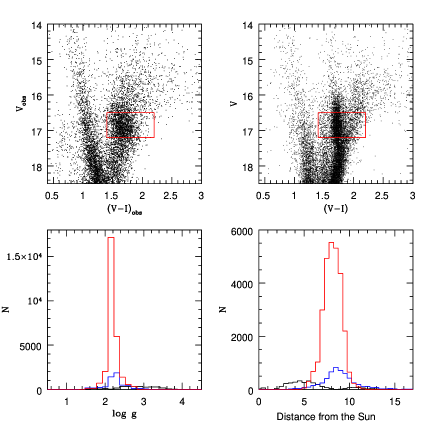
Figure 2: The two upper panels show the (V,(V-I)) colour-magnitude diagrams of our field in Baade’s window, as observed (left) and simulated by the Besançon model (right). The red boxes in these panels show the sample selection. On the lower part of the figure, the distributions in gravities (left) and distances (right) of model stars falling in the selection box are presented, separated into their parent populations: bulge (red), thin disc (black) and thick disc (blue). The low level of expected contamination of our bulge red clump sample is evident on these distributions. Note also that, while the thin disc contaminants lie in the foreground, thick disc contaminants are located in the very inner regions of the Galaxy, at distances similar to the bulge red clump population.

3 Determination of stellar parameters

3.1 Photometric parameters

Photometric temperatures were determined from the V-K, V-H and V-J colours using the calibrations of Ramírez & Meléndez (2005) and their extinction law with $\rm E(B-V)=0.55$ to correct for reddening.

The photometric gravities were calculated from the following equation:

$$\rm log\left(\frac{g}{g_{\odot}}\right)=log\left(\frac{M}{M_{\odot}}\right)-0.4\left(M_{Bol,\odot}-M_{Bol,\ast}\right)+4log\left(\frac{T_{eff}}{T_{eff,\odot}}\right)$$ (1)

with $\rm M_{Bol,\odot}=4.72$ mag, $\rm T_{eff,\odot}=5770$ K, $\rm logg_{\odot}=4.44$ dex for the Sun and $\rm M=0.8M_{\odot}$ for the bulge stars. The bolometric magnitude was computed from the V magnitude and the bolometric correction calibrations of Alonso et al. (1999) assuming that all stars were bulge members, at 8 kpc from the Sun (Reid, 1993).

Despite the use of infrared bands, both photometric $\rm T_{eff}$ and $\log g$ values are affected by the presence of the differential reddening but show a different sensitivity. In the Baade’s Window, the reddening spread is of the order of 0.15 mag on V-I leading to $\rm\sim$200K uncertainties on $\rm T_{eff}$ and $\rm\sim$0.05 dex on $\log g$. Therefore the photometric temperature (mean value from the V-K, V-H and V-J colours) was only used as an initial value in the stellar parameter determination procedure (see Sect. 3.3). The main source of uncertainty in the $\log g$ determination is the distance of the star. Assuming that all sample stars are at the mean bulge distance to the Sun can lead to an error up to 0.25 dex on $\log g$. However, on the whole sample, the previous uncertainty value remain lower than those expected from a $\log g$ deduced from the ionisation equilibrium. This is mainly due to uncertainties on the Fe II abundances coming from uncertainties in the equivalent widths measurements (continuum placement, blends) and on the $\log\,gf$ values of the Fe II lines (see Lecureur et al. (2007)). At GIRAFFE resolution, the previous source of uncertainties become larger and the photometric gravity was used as a final value. We also note that the $\rm T_{eff}$ value influences the photometric $\log g$: a change of $\rm\sim 200$ K can lead to changes on $\log g$ up to 0.15 dex for the cooler stars. Then, the $\log g$ value were recomputed at each step of the stellar parameters determination procedure taking into account the change on $\rm T_{eff}$.

3.2 Spectroscopic parameters

3.2.1 EWs measurement, atmospheric models and codes

The equivalent widths (EWs) for selected Fe I and Mg I lines were measured using the automatic code DAOSPEC (Stetson & Pancino, 2008). The synthetic spectra were computed using the LTE spectral analysis code “turbospectrum” (described in Alvarez & Plez 1998) and the abundances from EWs were derived using the Spite programs (Spite, 1967, and subsequent improvements over the years) with for both codes the new MARCS models (Gustafsson et al., 2008).

3.2.2 The iron linelist

The iron linelist from Lecureur et al. (2007) was used for the stellar parameter determination. This linelist was established in the following way: as a starting point, we used the linelist from Zoccali et al. (2004) with $\log\,gf$ values extracted from the NIST database (Ralchenko et al., 2008). By computing synthetic spectra in the stellar parameters range of the red clump stars, we rejected the iron lines blended up to 10% of the equivalent width. Finally, for the remaining iron lines, the $\log\,gf$ values were adjusted in order that each line gives an abundance of 0.30 dex from the EW measured on the observed spectrum of $\mu$Leo with the following stellar parameters: $\rm T_{eff}$ $=4540$ K, $\log g$ $=2.3$ dex, and $\xi$ $=1.3$ km s^-1. The spectrum of $\mu$Leo was obtained at the Canada-France-Hawaii Telescope with the ESPaDOnS spectropolarimeter (resolution R$\rm\sim$80000 and S/N per pixel $\rm\sim 500$) and processed using the “Libre ESpRIT” data reduction package (Donati et al., 1997).

Restricted to the wavelength ranges of H13+H14, the linelist contains 48 Fe I lines (92 initially). We checked the consistency of this reduced linelist on Arcturus and the Sun but also on the 12 red clump stars observed with GIRAFFE and UVES. The same parameters were found for Arcturus with the reduced and total linelists : $\rm T_{eff}$ $=4300$ K, $\log g$ $=2.5$ dex, $\xi$ $=1.5$ $\rm kms^{-1}$ and [Fe/H] $=-0.52$ dex. For the Sun, we obtained $\log g$ $=4.4$ dex, $\xi$ $=1.5$ km s^-1 but $\rm T_{eff}$$=5877$ K, ie increased by 100 K to fullfill the excitation equilibrium criterium. However, this has no impact on the deduced metallicity. For the 12 red clump stars, a new determination of the stellar parameters has been performed with the reduced linelist from the EWs measured on the UVES spectra with the same method as described in Lecureur et al. (2007). On the mean, the difference on the $\rm T_{eff}$ values are null with a dispersion of 100 K, lower than the uncertainties. The $\xi$ resulting from the use of the reduced linelist are slightly lower (0.1 km s^-1) than the ones found with the total linelist which translates into [Fe/H] values higher (0.1 dex) than the previous ones. However, these systematics are smaller than the uncertainties found on the individual values and let us conclude that the stellar parameters determination from the reduced line is reliable.

3.2.3 The microturbulence velocity determination

In Lecureur et al. (2007), $\xi$ was determined so that lines of different observed EWs give the same iron abundance. However, the observed EW values are sensitive to uncertainties due to either the quality of the spectra (S/N, resolving power) or the analysis method (continuum placement, FWHM fittings, … ) which translates to correlated uncertainties on the corresponding [Fe i/H]. This correlation between [Fe i/H] and observed EWs uncertainties leads to a bias towards higher $\xi$ as mentioned by Magain (1984).

In order to estimate this effect on the GIRAFFE sample, we performed simulations of the observed EWs and measured $\xi$ for each simulation. This procedure was applied to the star BWc-2 (a star representing well our sample: $\rm T_{eff}$ $\rm=4656$ K, $\log g$ $\rm=2.30$ dex, $\xi$ $\rm=1.5$ km s^-1 and $\rm[{Fe\textsc{I}}/H]=0.03$). We simulated 1000 stars by randomly drawing a set of Fe I lines EWs ($\rm EWs_{rand}$) around the expected EWs ($\rm EWs_{exp}$) with a standard deviation $\rm\sigma=\delta_{EWs}$ (given by DAOSPEC). For each 1000 simulated stars, Fe I abundances ($\rm[{Fe\textsc{i}}/H]_{rand}$) and corresponding uncertainties were computed from the random EWs using the stellar atmosphere model adopted for BWc-2. And $\xi$ was modified to minimise the slope p of $\rm[{Fe\textsc{i}}/H]_{rand}$ versus $\rm EWs_{rand}$ such that $\rm\left|p\right|<\sigma_{p}$, with $\rm\sigma_{p}$ the uncertainty on p. The simulation results are shown in Fig. 3. The systematic effect on the determination of $\xi$ using the observed EWs is clearly illustrated by the $\xi$ distribution histogram. In the mean, $\xi$ has to be increased by $\rm 0.10\pm 0.11$ km s^-1 leading to a corresponding systematic effect on the mean $\rm[{Fe\textsc{I}}/H]$ abundance which decreases by $\rm 0.06\pm 0.08$ dex.

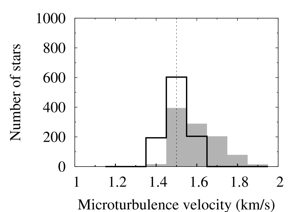
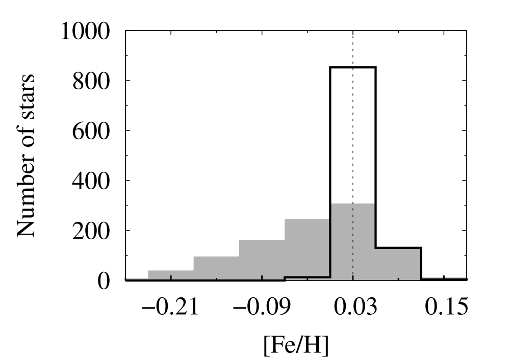
Figure 3: Results of the simulations for the star BWc-2 ($\rm T_{eff}$ $\rm=4656$ K, $\log g$ $\rm=2.30$ dex, $\xi$ $\rm=1.5$ km s^-1 and $\rm[{Fe\textsc{I}}/H]=0.03$). Left panel: Histogram of $\xi$ values found with the observed EWs (shaded histogram) and theoretical EWs (black line). Right panel: Histogram of the mean $\rm[{Fe\textsc{I}}/H]$ abundances. The correlation between uncertainties in observed EWs and the Fe I abundances leads to a systematic overestimate of $\xi$ determined from the abundances versus observed EWs plot. This overestimate is not significant anymore with the use of theoretical EWs.

This systematic effect can be suppressed using an abscissa linked to the observed EW but not affected by random errors. Magain (1984) suggested to use the expected EWs (computed from the adopted stellar atmophere model and some assumed values of $\xi$) and proposed a scheme where the slope of $\rm[{Fe\textsc{i}}/H]$ versus $\rm EWs_{exp}$ is minimised to deduce $\xi$. Such $\xi$ values are then free from bias EW abundance error correlations. This scheme was applied to the previously simulated sample. As clearly illustrated by the Fig. 3, the systematic effect on $\xi$ is not significant anymore: the mean $\xi$ value is of $\rm 1.50\pm 0.06$ km s^-1 and the corresponding mean $\rm[{Fe\textsc{I}}/H]$ value is of $\rm 0.02\pm 0.03$ dex.

However, this method can introduce another type of bias on $\xi$ (and thus on [Fe/H]) if the $\rm EWs_{exp}$ are computed from an atmosphere model that is far from reality. In particular, [Fe/H] needs to be known to $\rm\sim 0.07$ dex. For this reason, [Fe/H] was estimated as well as possible before $\xi$ was finally constrained.

3.3 Final stellar parameters determination

Starting with the photometric temperature, the final $\rm T_{eff}$ was determined iteratively by requiring the excitation equilibrium on Fe I lines (no variation of [Fe i/H] with the excitation potential of the line $\rm\chi_{ex}$. $\xi$ was constrained requiring no trend in the Fe I abundance as a function of the expected EW of the lines. At each step of the iteration on $\xi$, we checked that the metallicity of the atmophere model was the same as the one derived from the average Fe I abundance. As explained in Sect. 3.1, the photometric gravity was adopted as a final value and recomputed at each step of the iteration taking into account the change in $\rm T_{eff}$ and [Fe/H]. Stellar parameters and [Fe/H] values were finally obtained for 219 red clump stars of the initial sample (228 stars), and are reported in Table 2, available at the CDS (the first lines of the table are reproduced in the printed version).

This method was also applied to the UVES sample of Lecureur et al. (2007), using their full linelist, leading to new stellar parameters for each star of the sample. Fig. 4 shows the comparison between the new stellar parameters obtained with the new $\xi$ determination method and the “old” ones. There is no significant change in $\rm T_{eff}$ values, the difference between old and new values is of $\rm-34\pm 119$ K. As expected with this new method, $\xi$ values are on the mean found systematically lower of $\rm 0.12\pm 0.14$ km s^-1 which translates into [Fe/H] values systematically higher of $\rm 0.10\pm 0.09$ dex. Compared to the whole sample, the red clump stars are more sensitive to the change of $\xi$ determination with a mean difference between old and new values which reaches 0.25 km s^-1. This can be explained by lower S/N for these stars compared to the total sample and consequently higher uncertainties on the EWs and corresponding Fe I abundances making these stars more sensitive to the bias affecting the $\xi$ determination from the observed EWs.

Table 2: Adopted stellar parameters and measured [Fe/H] and [Mg/H] in the sample stars.

ID	$\rm T_{eff}$	$\log g$	$\xi$	[Fe/H]	$\sigma_{\rm Fe}$(low)	$\sigma_{\rm Fe}$(up)	[Mg/H]	$\sigma_{\rm Mg}$(low)	$\sigma_{\rm Mg}$(up)
	K	dex	$\rm kms^{-1}$	dex	dex	dex	dex	dex	dex
BWc-1	4528	2.09	1.4	0.29	0.14	0.13	0.34	0.08	0.08
BWc-2	4556	2.25	1.4	0.04	0.10	0.21	0.29	0.10	0.10
BWc-3	4713	2.23	1.5	0.33	0.17	0.28	0.42	0.15	0.15
BWc-4	4912	2.28	1.4	0.01	0.10	0.19	0.26	0.10	0.10
BWc-5	4636	2.21	1.5	0.58	0.12	0.33	0.63	0.14	0.14
BWc-6	4769	2.19	1.2	-0.17	0.17	0.30	-0.00	0.19	0.19
BWc-7	4769	2.19	1.2	-0.17	0.17	0.30	-0.00	0.19	0.19
BWc-8	4810	2.31	1.4	0.49	0.15	0.17	0.47	0.09	0.09
BWc-9	4685	2.21	1.5	0.17	0.12	0.24	0.21	0.12	0.12
BWc-10	4690	2.13	1.5	-0.13	0.14	0.24	0.20	0.11	0.11
…	…	…	…	…	…	…	…	…	…

Figure 4: Comparison of the stellar parameters ([Fe/H], $\xi$ and $\rm T_{eff}$) obtained with the new $\xi$ determination method (NEW) and those published in Lecureur et al. (2007) (OLD). The black dots represent the RGB stars and the open circle the red clump stars. The black line shows the mean difference and the dotted lines the $\rm\pm 1\sigma$ dispersion. With the new method, the $\xi$ values are systematically lower which implies [Fe/H] systematically higher.

3.4 The stellar parameters uncertainties

For each star of the red clump sample, an estimate of the uncertainty on [Fe/H] has been computed from the uncertainties on the stellar parameters. The uncertainties on $\rm T_{eff}$ and $\xi$ have been evaluated from the uncertainties on the Fe I line EWs given by DAOSPEC which translate into uncertainties in Fe I abundances derived from the EWs. These individual uncertainties on the Fe I lines were considered in the least squares line fit to the points in the ($\rm\chi_{ex},[{Fe\textsc{I}}/H]$) plane to fix $\rm T_{eff}$ and in the ($\rm EWs,[{Fe\textsc{I}}/H]$) plane to fix $\xi$ and are contained in the error on the line slope.

Keeping a fixed $\xi$, $\rm T_{eff}$ upper and lower allowed boundaries were estimated by letting the slope p reaches its 1 $\rm\sigma$ uncertainty: $\rm p\pm\sigma_{p}$. The thus determined boundaries are called $\rm T_{eff}$_,up and $\rm T_{eff}$_,lo and the corresponding uncertainties on $\rm T_{eff}$ $\rm\sigma_{up}$($\rm T_{eff}$) and ($\rm\sigma_{lo}$($\rm T_{eff}$) respectively. Note that these temperature uncertainties need not to be symmetric. In fact, for the 219 red clump stars, we found: $\rm\sigma_{sup}$($\rm T_{eff}$)$\rm=180\pm 90$ K and $\rm\sigma_{inf}$($\rm T_{eff}$)$\rm=220\pm 90$ K and half of the sample shows asymmetric uncertainties on $\rm T_{eff}$ which can reach 200 K. Lower ($\rm\sigma_{lo}$($\xi$)) and upper ($\rm\sigma_{up}$($\xi$)) uncertainty values on $\xi$ have been estimated with the same principle fixing the $\rm T_{eff}$ value. Contrary to the $\rm T_{eff}$’s, these uncertainties are quasi symmetric with $\rm|\sigma_{inf}$($\xi$)$\rm|=|\sigma_{sup}$($\xi$)$\rm|=0.21\pm 0.08$ km s^-1.

A modification in $\rm T_{eff}$ (or in $\xi$) value induces a change in [Fe/H] which varies from star to star depending on the initial stellar parameters but also on the quality of the EW measurement (S/N ratio, continuum placement, … ). As illustrated by Fig. 5, changing $\rm T_{eff}$ by 200 K implies a change of [Fe/H] around 0.10 dex for the coolest and more metallic stars of the sample and around 0.20 dex for the hotter and less metallic stars. Changes of $\xi$ by 0.2 km$\rm s^{-1}$ lead to similar variations in the [Fe/H] value: around 0.10 dex for the coolest and more metallic stars of the sample and around 0.16 dex for the hotter and less metallic stars. Overall in our 219 clump stars sample, the uncertainties on [Fe/H] associated to $\rm T_{eff}$ uncertainties are of $\rm 0.15\pm 0.07$ dex on the mean, and those associated to $\xi$ uncertainties, of $\rm 0.16\pm 0.06$ dex. The individual values are reported in the Table 3, available at the CDS in its entirety (the first lines of the table are reproduced in the printed version).

Figure 5: Variation in the resulting [Fe/H] with increasing $\rm T_{eff}$ by 200 K (lower panels) and $\xi$ by 0.2 km$\rm s^{-1}$ (upper panels) as a function of the initial $\rm T_{eff}$ (left panels) and of the initial [Fe/H] value (right panels). The hotter and less metallic stars are the most sensitive to a modification of $\rm T_{eff}$ whereas the cooler and more metallic stars are the most sensitive to a modification of $\xi$.

The uncertainty associated with [Fe/H] were computed with the formalism described in McWilliam et al. (1995) taking into account the errors on the model atmosphere stellar parameters $\rm T_{eff}$ and $\xi$ and the errors on the Fe I line EW measurements. Errors on [Fe/H] coming from the $\log g$ value or the metallicity adopted to compute the stellar atmosphere model were found to be negligible compared to the other sources. Finally, the variance on [Fe/H], $\rm\sigma^{2}(Fe)$, can be written as:

$$\rm\sigma^{2}(Fe) = \left(\frac{\partial\epsilon}{\partial W}\right)^{2}\sigma^{2}_{W}+\left(\frac{\partial\epsilon}{\partial T}\right)^{2}\sigma^{2}_{T}+\left(\frac{\partial\epsilon}{\partial\xi}\right)^{2}\sigma^{2}_{\xi}$$ (2)

$$+2\left(\frac{\partial\epsilon}{\partial T}\right)\left(\frac{\partial\epsilon}{\partial\xi}\right)\sigma_{T,\xi},$$

with $\epsilon$ the Fe abundance, $\rm\sigma^{2}_{W}$, $\rm\sigma^{2}_{T}$ and $\rm\sigma^{2}_{\xi}$ the variance in the EWs measurement, $\rm T_{eff}$ and $\xi$, respectively and $\rm\sigma_{T,\xi}$, the covariance between $\rm T_{eff}$ and $\xi$. The covariances between the EW measurements and the stellar parameters $\xi$ or $\rm T_{eff}$ are null because these variables are independent. The terms $\rm\left(\frac{\partial\epsilon}{\partial T}\right)^{2}\sigma^{2}_{T}$ and $\rm\left(\frac{\partial\epsilon}{\partial\xi}\right)^{2}\sigma^{2}_{\xi}$ were computed as explained in the previous paragraph. The variance in the EW measurements and the associated uncertainty on [Fe/H] were estimated from the line to line dispersion divided by the number of lines. The covariance between $\rm T_{eff}$ and $\xi$ were approximated by measuring the variation in the slope fixing $\rm T_{eff}$ (resp. $\xi$) due to changes in $\xi$ (resp. $\rm T_{eff}$).

The total upper and lower uncertainty values on [Fe/H] and [Mg/H] computed from equation 2 are reported in Table 2, while Table 3 details the different contributions of the stellar parameter uncertainties ($\sigma_{\xi}$ and $\sigma_{\rm T}$) propagated onto the abundances ($\sigma_{\xi}(\rm Fe)$). On the whole red clump sample (219 stars), and as illustrated in Fig. 6, the lower values range from 0.04 to 0.35 dex with a median value of $\rm 0.17\pm 0.05$ and show no trend with metallicity. The upper values are systematically higher with a median value of $\rm 0.24\pm 0.08$ and show an increase with the metallicity reaching 0.5 dex for supersolar metallicity stars.

Table 3: Errors in stellar parameters and associated errors on Fe for the sample stars.

					lower					upper
ID	$\rm T_{eff}$	$\log g$	$\xi$	[Fe/H]	$\sigma_{\xi}$	$\sigma_{\xi}(\rm Fe)$	$\sigma_{\rm T}$	$\sigma_{\rm T}(\rm Fe)$		$\sigma_{\xi}$	$\sigma_{\xi}(\rm Fe)$	$\sigma_{\rm T}$	$\sigma_{\rm T}(\rm Fe)$
	K	dex	$\rm kms^{-1}$	dex	$\rm kms^{-1}$	dex	K	dex		$\rm kms^{-1}$	dex	K	dex
BWc-1	4528	2.09	1.4	+0.29	-0.10	+0.07	+150	+0.10		+0.20	-0.16	-200	-0.10
BWc-2	4556	2.25	1.4	+0.04	-0.20	+0.19	+100	+0.08		+0.10	-0.07	-150	-0.07
BWc-3	4713	2.23	1.5	+0.33	-0.20	+0.16	+300	+0.23		+0.30	-0.22	-50	-0.03
BWc-4	4912	2.28	1.4	+0.01	-0.20	+0.19	+100	+0.10		+0.10	-0.06	-100	-0.09
BWc-5	4636	2.21	1.5	+0.58	-0.30	+0.30	+300	+0.17		+0.10	-0.12	-400	-0.16
BWc-6	4769	2.19	1.2	-0.17	-0.20	+0.15	+300	+0.26		+0.20	-0.13	-200	-0.15
BWc-7	4769	2.19	1.2	-0.17	-0.20	+0.15	+300	+0.26		+0.20	-0.13	-200	-0.15
BWc-8	4810	2.31	1.4	+0.49	-0.10	+0.10	+150	+0.13		+0.10	-0.07	-200	-0.14
BWc-9	4685	2.21	1.5	+0.17	-0.20	+0.20	+150	+0.13		+0.20	-0.14	-200	-0.15
BWc-10	4690	2.13	1.5	-0.13	-0.20	+0.15	+200	+0.18		+0.30	-0.21	-200	-0.14
…	…	…	…	…	…	…	…	…		…	…	…	…

Figure 6: Left panels: upper and lower errors on [Fe/H] as a function of [Fe/H] for the 219 red clump stars. The upper values increase with the metallicity with mean values around 0.3 dex for the most metallic stars. The lower values show no trend with [Fe/H] with a median value of 0.17 dex for the whole sample. Right panels: upper and lower errors on [Mg/H] as a function of [Mg/H] for the 162 red clump stars selected from the total sample. At low [Mg/H], the abundance errors are dominated by the line measurement rather than stellar parameter uncertainties because

the Mg triplet lines become very weak.

We also mention that a mean error in [Fe/H] was also estimated by Zoccali et al. (2008) by comparing the measured metallicities in the 50 stars (RGB and red clump stars of the Lecureur et al. (2007)’s sample) observed both with GIRAFFE and UVES. They found no systematic offset on the [Fe/H] values with a scatter of 0.16 dex, a value in agreement with the previous estimates from the total GIRAFFE red clump sample.

3.5 Magnesium abundances

The Mg abundances were determined from the 6319Å triplet using spectral synthesis fitting. The synthetic spectra were computed using the LTE spectral analysis code “turbospectrum” (described in Alvarez & Plez, 1998) and the molecular and atomic linelists described in Lecureur et al. (2007). In short, we recall that the atomic linelist is the one of the VALD database (Kupka et al., 1999, and references therein) with (i) solar astrophysical $\log\,gf$ -values for the three lines of the Mg triplet and (ii) the $\rm\lambda$ 6318.1 Å Ca I autoionisation line broadening adjusted in order to reproduce the Ca I dip in the Sun, Arcturus and $\mu$Leo. The molecular line lists included in our syntheses are the following: C₂ (¹²C¹²C and ¹²C¹³C) Swan system (A-X); CN (¹²C¹⁴N and ¹³C¹⁴N) red system (A-X); TiO $\gamma$ and $\gamma^{\prime}$ systems Plez (1998). In and near the triplet, the $\log\,gf$values of some CN lines were modified in order to obtain the same Mg abundance from the three lines of the triplet in the three reference stars.

3.5.1 In the UVES stars: new determination

Adopting the new stellar parameters and metallicities (see Sect. 3.3), the Mg abundances were determined for the UVES stars as described in Lecureur et al. (2007) with a Ca abundance computed from the following relation: $\rm[Ca/Fe]=-0.20[Fe/H]+0.06$. This linear relation was obtained on the UVES sample by a least square fit to the [Ca/Fe] values deduced from EWs.

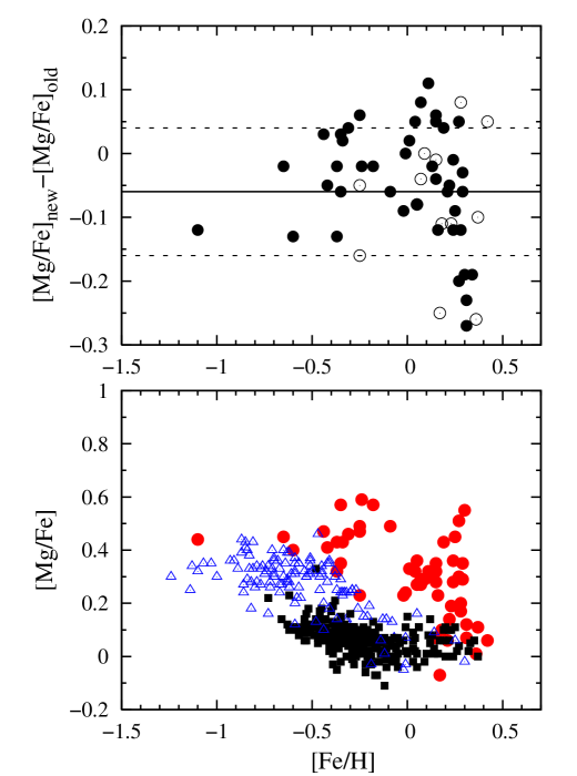
Figure 7: Upper Panel: Difference on [Mg/Fe] found for the UVES red clump (open circle) and RGB stars (full circle) with the old and new set of parameters as a function of the new metallicities. The black line shows the mean value of this difference (-0.06) and the two dotted lines shows the $\rm\pm 1\sigma$ dispersion ($\rm\sigma=0.10$). Lower Panel: [Mg/Fe] in the UVES bulge stars (red points, computed with the new stellar parameters) compared with the [Mg/Fe] in the thin (black squares) and thick (blue triangles) discs stars from Bensby et al. (2004, 2005); Reddy et al. (2006). For metallicities from -0.4 to 0.1, the bulge stars show higher [Mg/Fe] values than in the two discs.

The mean difference in [Mg/H] between the two determinations is very small (as expected because [Mg/H] is not sensitive to a change of $\xi$): $\rm[Mg/H]_{new}-[Mg/H]_{old}=0.03\pm 0.06$ dex but becomes more significant on [Mg/Fe] with $\rm[Mg/Fe]_{new}-[Mg/Fe]_{old}=-0.06\pm 0.10$ dex (see Fig.7). However, the global trend of [Mg/Fe] vs [Fe/H] is almost not affected by this difference as illustrated by Fig.7 which shows the new [Mg/Fe] in the bulge stars and the [Mg/Fe] found in the thin and thick discs stars by Bensby et al. (2004, 2005) and Reddy et al. (2006). In the lower metallicities range ([Fe/H]$\rm<-0.4$), the bulge stars are not as separated from the thick disc stars than they were in (Lecureur et al., 2007, see Fig.6) with [Mg/Fe] values in bulge stars similar to the highest values found in the thick disc stars. For $\rm-0.4\lesssim[Fe/H]\lesssim 0.1$, the bulge still shows higher [Mg/Fe] values than those found in both discs. At higher metallicities, the dispersion has slightly decreased (this comes mainly from our use of the linear relation to compute the Ca abundance rather than relying on individual –more uncertain– values for each star) but remains high, with [Mg/Fe] values from thin disc values ($\rm[Mg/Fe]\sim 0.1$) to 0.55. The conclusions drawn by Lecureur et al. (2007) from the [Mg/Fe] values are still valid with the [Mg/Fe] computed from the new stellar parameters. The abundances of O, Al and Na in the UVES stars will also be updated using these new stellar parameters and be published and discussed in a future paper.

3.5.2 In the GIRAFFE stars

From the total red clump sample (219 stars), we selected stars according to their uncertainties on the [Fe/H] values in order to exclude stars for which Mg would be measured with too large uncertainties (mainly stars with low S/N spectra). Only stars with $\rm\sigma_{up}(Fe)<0.30$ were kept providing a new subsample of 162 stars. To compute the synthetic spectrum, the abundances of C,N, O and Ca are needed for each star of the GIRAFFE sample. As a result from the decrease in spectral resolution, the C, N and O indicators measurable in the UVES spectra are either nondetectable in the GIRAFFE spectra or would lead to large uncertainties in the resulting abundances, mainly due to uncertainties in the continuum placement ($\rm\sim 0.5$ dex on [C/H] and $\rm\sim 0.3$ dex on [O/H]). Therefore, the synthetic spectra were computed with the mean values, [C/Fe]=-0.04 and [N/Fe]=+0.43, found in the UVES stars sample. The O abundance was deduced from the following linear relation: [O/Fe]=-0.56[Fe/H]+0.22 fitted by least squares to the [O/Fe] values found for the UVES stars sample of Zoccali et al. (2006). The Ca abundance was computed as in Sect. 3.5.1.

Each observed spectrum was first normalised using the continuum found by DAOSPEC. The continuum was then adjusted by a visual inspection of a 10 Å wavelength interval centred on the triplet. In order to well identify the possible absorption from the CN lines and/or from the Ca I line, two other synthetic spectra were overlaid: (i) one spectral synthesis only with the molecular lines and (ii) one spectral synthesis only with the Ca I. This visual analysis also permits to flag or reject some stars from the final Mg measurement for one of the following reasons: (i) presence of telluric lines affecting the Mg measurement, (ii) a too low signal to noise ratio in the Mg region which can affect the continuum placement and (iii) a strong disagreement between observed and synthetic spectra.

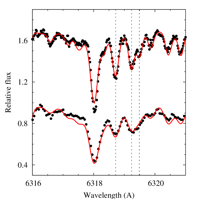
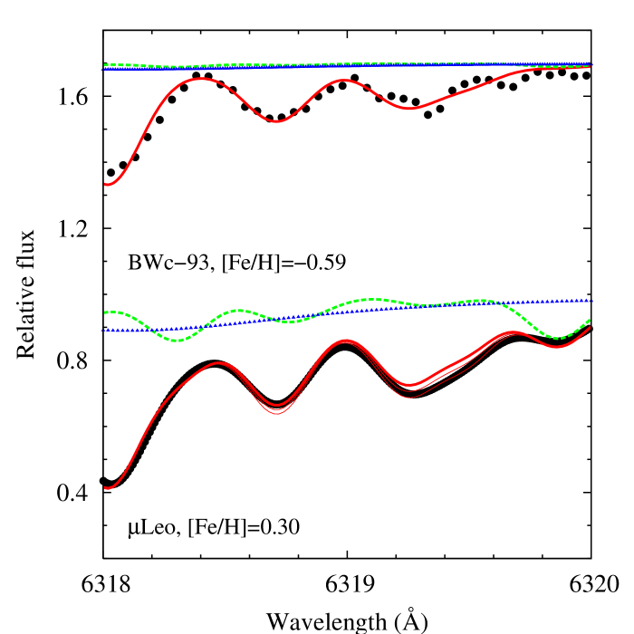
Figure 8: Left Panel: Observed spectrum (black points) around the Mg I triplet for the BWc-1 red clump star obtained with GIRAFFE (lower spectrum) and UVES (upper spectrum). The red lines represent the synthetic spectra computed with [Mg/H]=+0.34 and [Mg/H]=+0.38 respectively for GIRAFFE and UVES convolution. Right Panel: Comparison of observed (black points) and synthetic spectra (red lines) computed with [Mg/H]=-0.16 for the red clump star BWc-93 and [Mg/H]=+0.42,+0.32,+0.22 for $\mu$Leo. The blue dotted lines and the green thick dashed lines represent the absorption of the Ca I line and of the CN lines respectively. In BWc-93, the contamination by the Ca I and CN lines is negligible and the agreement between the observed and synthetic spectra is found for the three lines of the triplet. In $\mu$Leo, the abundance deduced from the Mg I line at 6318.72 Å is 0.2 dex lower than the one deduced from the two redder lines of the triplet.

At GIRAFFE resolution, blends between the two redder lines of the triplet and between the Mg I line at 6318.72 Å and the Fe I line at 6318.1 Å become more important as illustrated by Fig.8. This figure also shows that linelist uncertainties do not have a significant impact on the Mg abundance determination from UVES spectra, but become larger at GIRAFFE resolution and can affect the Mg value. More specifically, in the synthetic spectra, the absorption around 6318.2 Å is overestimated and at GIRAFFE resolution, the left wing of the Mg I line at 6318.72 Å become more contaminated leading to an underestimation of the Mg abundance deduced from this line. These effects were measured on $\mu$Leo by comparing the observed spectrum convolved to the GIRAFFE resolution with the synthetic spectrum computed with the stellar parameters, C, N, O and Ca abundances for $\mu$Leo from Lecureur et al. (2007) and different Mg abundances (see Fig.8, right panel). The abundance deduced from the two redder lines of the triplet is [Mg/H]=0.42, whereas the abundance deduced from the line at 6318.72 Å is 0.2 dex lower.

Due to the previous considerations, for each star of the subsample, two estimations of the Mg abundance were computed by minimising the $\rm\chi^{2}$ values between normalised observed and synthetic spectra on a wavelength domain restricted (i) to the region covered by the two redder lines ($\rm[Mg/H]_{2Lines}$) and (ii) to the region covered by the three lines of the Mg triplet ($\rm[Mg/H]_{triplet}$). On the whole sample, the Mg abundance deduced from the triplet is on the mean 0.05 dex lower than the one deduced from the two redder lines with a dispersion of 0.06 around the mean. For the less metallic stars, the difference $\rm[Mg/H]_{2Lines}-[Mg/H]_{triplet}$ can be negative and the mean difference is null. In this metallicity range, the triplet absorption weakens and the abundance deduced from the two redder lines becomes more sensitive to uncertainties (S/N, continuum placement). For stars with $\rm[Fe/H]>-0.4$ dex, the difference starts to be positive and increases with the metallicity of the star to reach 0.15 dex for the more metallic stars. Moreover, at supersolar metallicities, the [Mg/Fe] values deduced from the triplet are more dispersed than those deduced from the two redder lines. In our red clump GIRAFFE sample, to allow for both these considerations, we finally adopted the [Mg/H] value deduced from the triplet for the stars with $\rm[Fe/H]<-0.4$ dex and the value deduced from the two redder lines of the triplet for the stars with $\rm[Fe/H]>-0.4$ dex.

In order to evaluate the Mg determination for the red clump stars, we compared the Mg abundances found from the GIRAFFE spectra ($\rm[Mg/H]_{GIR}$) with those found from the UVES spectra ($\rm[Mg/H]_{UVES}$) for the stars observed with both instruments (see Fig. 9). To increase the statistics of the comparison, we also computed with the same method the Mg abundances in 30 RGB stars of Lecureur et al. (2007)’s sample from the GIRAFFE spectra with the stellar parameters determined by Zoccali et al. (2008). For the total sample (44 stars), a systematic difference between the two determinations is found: $\rm[Mg/H]_{GIR}-\rm[Mg/H]_{UVES}=-0.06\pm 0.16$ dex which does not depend on the metallicity. This difference is small, and can be mainly explained by the resolution decrease which affects the Mg determination via uncertainties in the continuum placement and/or uncertainties in the atomic and molecular linelist that affect the line fitting differently at different resolutions. Both red clump and RGB stars show the same behaviour.

However, in terms of comparison with abundances found in the discs, this small difference can become significant. Fig. 9 shows the [Mg/Fe] ratios found from GIRAFFE and UVES spectra of the same stars. The two sets of points show a similar global trend, although for $\rm-0.3<[Fe/H]<0$, $\rm[Mg/Fe]_{GIR}$ ratios are closer to those found in thick discs stars at the same metallicity than the $\rm[Mg/Fe]_{UVES}$ were. At higher metallicity ($\rm[Fe/H]>0.2$), the dispersion on $\rm[Mg/Fe]_{GIR}$ values is considerably lower than that of $\rm[Mg/Fe]_{UVES}$. We attribute the larger dispersion found from the UVES spectra to the result of the lower S/N ratios for these spectra. From both sets of measurements, the bulge stars have [Mg/Fe] ratios on the mean higher than those of the thin disc stars, but half of the stars fall within the thin disc trend from the GIRAFFE measurement, which was not the case from the UVES measurement. The [Mg/Fe] trend will be further discussed in Sect. 4.1 for the total red clump sample, but we would like to note at this point that the previous sample of Lecureur et al. (2007) plotted here was a mix of red clump (13) in Baade’s Window and RGB stars (44) coming from four different fields located at Galactic latitudes of $-3^{\circ}$, $-4^{\circ}$ (Baade’s Window), $-6^{\circ}$ to $-12^{\circ}$. Among these fields, some are expected to be more contaminated by foreground Galactic discs (thin and thick), and this could partly explain the difference between the sample studied in Lecureur et al. (2007) and the pure Baade’s Window sample studied in the present paper.

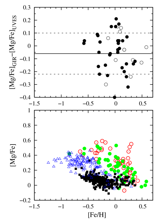
Figure 9: Lower Panel: Comparison of the [Mg/Fe] found from GIRAFFE spectra (green filled circles) with [Mg/Fe] found from UVES spectra for 44 bulge stars of Lecureur et al. (2007)’s sample (open dotted circles). The thin (black filled squares) and thick (blue open triangles) discs abundances come from Bensby et al. (2004, 2005); Reddy et al. (2006). Upper Panel: Difference on [Mg/Fe] found from GIRAFFE and UVES spectra for 44 stars (red clump (open circle) and RGB stars (full circle)) observed with both instruments. The black line shows the mean value of this difference (-0.06) and the two dotted lines shows the $\rm\pm 1\sigma$ around ($\rm\sigma=0.16$).

3.5.3 [Mg/H] and [Fe/H] uncertainties for the red clump sample

The individual uncertainties on [Mg/H] and [Fe/H] were estimated from uncertainties associated with the $\rm\chi^{2}$ procedure ($\rm\sigma_{FIT}$), as well as the uncertainties linked to uncertainties on stellar parameters ($\rm T_{eff}$ and $\xi$  computed in Sect. 3.4). $\rm\sigma_{FIT}$ was computed using the $\rm\delta\chi^{2}=1$ contour. The uncertainty on [Mg/H] due to the uncertainty on $\rm T_{eff}$ and on $\xi$ were computed with the following relations: $\rm\sigma([Mg/H])_{T}=\left(\frac{d[Mg/H]}{dT}\right)\sigma(T)$ and $\rm\sigma([Mg/H])_{\xi}=\left(\frac{d[Mg/H]}{d\xi}\right)\sigma(\xi)$ with $\rm\sigma(T)$ and $\rm\sigma(\xi)$ the uncertainties on $\rm T_{eff}$ and $\xi$ respectively. $\rm\left(\frac{d[Mg/H]}{dT}\right)$ and $\rm\left(\frac{d[Mg/H]}{d\xi}\right)$ were estimated from the [Mg/H] dependance to the $\rm T_{eff}$ and $\xi$ variations found in the UVES stars (see table 10 of Lecureur et al., 2007). Errors arising from log g uncertainties (an error of 0.3 dex on log g corresponds to an error of 0.02 on average) were found to be negligible compared to the other sources.

4 Metallicity distributions

4.1 Raw metallicity distributions

4.1.1 [Fe/H] metallicity distribution

The resulting metallicity distribution (MD) for the 219 bulge red clump stars is shown in Fig. 10. The mean [Fe/H] value is $+0.05\pm 0.03$ dex and the full range of metallicities spans $\rm-1.13<[Fe/H]<0.71$ dex. The distribution is clearly asymmetric with a median [Fe/H] value of $0.19$ dex and shows a large proportion of metal rich stars: 65% with supersolar metallicities and 25% with $\rm[Fe/H]>0.38$ dex. For $\rm[Fe/H]>0.50$ dex, the number of stars decreases considerably.

The MD shows two low-level secondary peaks around [Fe/H] = $\rm-0.55$ and around [Fe/H] = $\rm-0.20$ dex, both with very low statistics. While the first remains whatever the size and centre of the histogram bins, the second results from a small accumulation of stars in a very narrow metallicity range around $\rm[Fe/H]=-0.20$ and therefore becomes more or less pronounced according to binning. We checked that this latter peak is not related to the two bulge globular clusters NGC6522 and NGC6528 that are close to the region: the former has an intermediate metallicity close to $-1$ (Terndrup et al., 1998), while the latter, with a mean metallicity of $-0.1$ (Zoccali et al., 2004) is too far from the observed window.

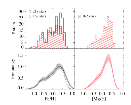
Figure 10: Upper left panel: distribution of [Fe/H] for the 219 bulge clump stars in the Baade’s window (thick histogram) and distribution of [Fe/H] for the 162 star subsample for which [Mg/H] is measured (hatched histogram). Upper right panel: distribution of [Mg/H] for the 162 bulge clump stars in the Baade’s window. Lower left panel: smoothed distribution of [Fe/H] derived from the upper panel, with its associated variability band. The initial metal rich side of the distribution (dashed line) has been stretched ((full line) to make it consistent with the error law and to achieve the deconvolution (see text). Lower right panel: smoothed distribution of [Mg/H] derived from the upper panel, with its associated variability band (see text).

Table 4: Statistics of the samples: the size $n$ (number of stars), the mean and median (in dex), the smoothing parameter $\hat{h}$ according to Sheather & Jones (1991) and the variability band width $\epsilon$.

Subsample	$n$	mean	median	$\hat{h}$	$\epsilon$
[Fe/H]	219	$0.05{\scriptstyle\pm 0.03}$	$0.16{\scriptstyle\pm 0.04}$	0.0881	0.0605
[Mg/H]	162	$0.14{\scriptstyle\pm 0.02}$	$0.21{\scriptstyle\pm 0.03}$	0.0871	0.0707

In order to investigate the significance of low-level secondary peaks, we estimate the probability density function (PDF) from the raw data, using a kernel estimator. This estimator is:

$$\hat{\Phi}(x)={1\over n}\sum_{i=1}^{n}{1\over h}\,K\left({x-X_{i}\over h}\right),$$ (3)

where $(X_{i})$ are the observed metallicities, $n$ is the sample size and $h$ is the window width, also called the smoothing parameter. We chose the kernel function $K$ to be a Gaussian distribution. The smoothing parameter $h$ in Eq. 3 is estimated using the scheme described by Sheather & Jones (1991). The estimator $\hat{h}$, as solution of the Eq. 12 in Sheather & Jones (1991), is given in Table 4 for each subsample.

The variability bands, as described by Bowman & Azzalini (1997, Chap 2.3), are computed to assess the significance of the modes in the derived distributions. In the case of a Gaussian kernel function, the variability band width around $\sqrt{\hat{\Phi}}$ is $\epsilon\approx{0.2656\,{\left(\hat{h}\,n\right)}^{-0.5}}$ (Bowman & Azzalini, 1997). The values are given in Table 4 and they are displayed in the lower panels in Fig. 10. More details about the smoothing method can be found in Royer et al. (2007, Sect. 4 and Appendix C).

As far as the secondary modes observed in the [Fe/H] histogram (Fig. 10) are concerned, the smoothed distribution together with the variability band indicate that the most deficient one, around $\textrm{[Fe/H]}=-0.55$ dex, is significant whereas the intermediate one, around $\textrm{[Fe/H]}=-0.20$ dex, is not and is rather part of a transition between the two main modes: around $\textrm{[Fe/H]}=0.35$ dex and $\textrm{[Fe/H]}=-0.55$ dex.

4.1.2 [Mg/H] metallicity distribution

With the analysis method described in Sect. 3.5, Mg abundances have been determined for a subsample of 162 red clump stars built by excluding stars with high uncertainties in the [Fe/H] value (only stars with $\rm\sigma_{up}(Fe)<0.30$ were kept). As illustrated in Fig. 10, the resulting [Fe/H] distribution has the same global shape than the one found before from the total sample, as was confirmed by a Kolmogorov-Smirnov test (D = 0.0793, p-value = 0.5996). The main difference between the two distributions is for $\rm[Fe/H]>0.2$ where our selection criteria has excluded a large number of stars, but the [Fe/H] distribution for the 162 stars still shows the same sharp decrease of the number of stars at very high metallicities.

The resulting [Mg/H] distribution is shown in Fig. 10. Compared to the [Fe/H] distribution, the [Mg/H] distribution is much narrower, ranging from [Mg/H] = $\rm-0.7$ to [Mg/H] = $\rm+0.6$. While the sample contains 25% of stars with $\rm[Fe/H]<-0.2$, those stars all have $\rm[Mg/Fe]>0$, which explains the lack of the metal poor tail of the [Mg/H] distribution. The mean and median values are higher in [Mg/H] than in [Fe/H]: 0.14 and 0.21 respectively (to be compared to 0.05 and 0.16). The distribution also shows two peaks: one around [Mg/H] = $\rm+0.3$ and a second less significant around $\rm[Mg/H]=-0.3$. For $\rm[MgH]>+0.3$, the number of stars decreases very abruptly. This characteristic has already been seen in the [Fe/H] distribution but is even more drastic on the [Mg/H] distribution. Moreover, we would expect this effect to be larger with the addition of the stars excluded by the selection. Indeed, the latter are mainly very high metallicity stars ($\rm[Fe/H]>0.2$) that should follow the same [Mg/Fe] trend as the other Fe-rich stars (see Fig.14) which have [Mg/Fe] abundances from $-0.1$ to $0.1$ and therefore they should populate the region where $\rm 0.1<[Mg/H]<0.3$. This effect will be discussed further in Sect. 5.

The smoothed distribution of [Mg/H] does not display any significant secondary mode, but the spread of the distribution is indeed smaller than the one observed for [Fe/H].

4.1.3 [Fe/H] distribution robustness

To further investigate the robustness of our iron MD against abundance undertainties, we rejected stars with high uncertainties in two different ways, and checked the consistency of the resulting MD: i) stars with $\rm\sigma_{lo}(Fe)\leqslant 0.22$ were kept; ii) stars with $\rm\sigma_{up}(Fe)\leqslant 0.28$ and $\rm[Fe/H]<0.20$ or $\rm\sigma_{up}(Fe)\leqslant 0.36$ and $\rm[Fe/H]\geq 0.20$ were kept, taking into account the increase of the $\rm\sigma_{lo}(Fe)$ uncertainty with metallicity (see Sect. 3.4 and Fig. 6). The two resulting distributions were found to be fully compatible with the total MD. Furthermore, to detect possible bias in the MD arising from the analysis method itself, we checked the robustness of the MD upon the difference between the spectroscopic and photometric $\rm T_{eff}$. The resulting MD (obtained for the stars with a temperature difference $\rm\leqslant 50$ K and $\rm\geqslant 150$ K) are also compatible with the total MD.

However, the decrease in the iron MD at the high-metallicity end (highlighted by the small number of stars with $\rm[Fe/H]>0.5$) is too sharp to be compatible with the expected measurement errors (see 3.4 and Fig. 6) and suggests that a bias against the highest [Fe/H] could be present. To show this, let us extract the stars from the MD with supersolar metallicities, as representative of the metal-rich peak of the distribution. First, using $\rm[Fe/H]>0$ as a lower cut-off, the cumulative distribution of supersolar metallicities is plotted in Fig. 11. Under the hypothesis that, even if the highest metallicities are biased, the median of the distribution of the metal-rich peak is conserved (which is the case if errors remain almost symetrical), this median (i.e. frequency = 0.5), corresponds to $\rm[Fe/H]=0.35dex$. This median is relatively robust to different cut-off values ($-0.1$ or $0.1$ dex) for defining the high-metallicity peak, for which we obtain respectively $\rm[Fe/H]=0.32$ and $0.36$ dex. The frequencies $0.16$ and $0.84$ respectively mark the 1-$\sigma$ positions from the median on the lower and upper sides of the distribution. These values, displayed in Fig. 11, show a clear asymetry: $\sigma_{\mathrm{left}}=0.21$ dex and $\sigma_{\mathrm{right}}=0.16$ dex. While $\sigma_{\mathrm{left}}$ is slightly larger than the median expected measurement error $\rm\sigma_{low,Fe/H]>0}$ of 0.17, allowing for a small astrophysical scatter, the $\sigma_{\mathrm{right}}$ is too small compared to the median expected error $\rm\sigma_{up,[Fe/H]>0}=0.24$ (Fig.6). The metal rich end of the [Fe/H] MD is thus too steep to be consistent with the expected dispersion of the measurements due to their observational uncertainties only. One possibility is that remaining degeneracies between $\xi$ $\rm T_{eff}$ and [Fe/H] introduce a bias in the metallicity estimates of the most metal-rich stars ($\rm[Fe/H]>0.35$) at the resolution a S/N of the present sample, preventing us to truly establish the underlying shape of the iron MD tail at high metallicities.

This bias is not detected in [Mg/H] though, for which the observed [Mg/H]distribution is compatible with the expected uncertainties, even if this distribution also displays a sharp cutoff at high metallicities. This is because the Mg lines used in the analysis are weak and do not suffer in the same way of $\xi$ $\rm T_{eff}$ degeneracies in the stellar parameter determination. As a result, the uncertainties on [Mg/H] are both smaller than those on [Fe/H] at high metallicities, and less assymetric. Another way to say this is that, since the error on [Mg/H] is dominated by actual line measurement errors (synthetic spectra fits in this case), the possible (small) bias in [Mg/H] at the highest metallicities is hidden.

To understand wether such a bias could indeed be present, we computed synthetic spectra of metal-rich (0. to +0.75dex) red clump stars, sliced and convolved them to the same wavelength domains, resolution and sampling as our observed GIRAFFE spectra. We added photon noise to the spectra to reproduce a set of spectra with S/N=100, 50, 40 and 30(100 realisations of the noise were generated for each synthetic spectrum and noise level). We then retrieved the stellar parameters and metallicity using the same method as for the bulge stars (equivalent width measurements and iteration on the stellar parameters). The results of these extensive simulations show that for supersolar metallicities, there is indeed a slight bias in the retrieved metallicities, although it is in the contrary direction than what would be suggested by the error analysis above: in the mean, very metal-rich stars are found slightly too metal-rich by our method. In the mean, a [Fe/H]=$+0.5$ star will be found $+0.14$ to $+0.17$ dex more metal-rich, whereas a [Fe/H]=$+0.25$ star will be found $+0.10$ to $0.14$ dex more metal-rich (the bias steadily growing with decreasing S/N from 100 to 30). At and below solar metallicities, the bias vanishes. Finally, we also confirmed this bias by performing the same test on the observed $\mu$Leo spectrum, degraded in resolution, wavelength coverage and photon noise. In this case, the bias is $+0.13$ at S/N=50 and $+0.18$ at S/N=30.

Based on these findings, we warn the reader that there may be a bias in the highest metallicity stars of the sample, although this bias is not understood well enough to be corrected.

Figure 11: The cumulative iron metallicity distribution for $\rm[Fe/H]>0$ (solid line). The median and the left and right standard deviations are derived from the frequency values, assuming Gaussian errors.

4.1.4 Comparison with the [Fe/H] distribution of RGB stars

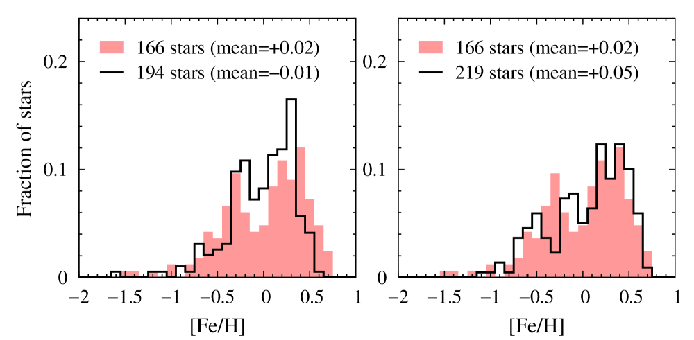
Figure 12: Iron metallicity distribution (MD) of RGB stars obtained with the automatic procedure (red shaded histogram) compared with the MD of Zoccali et al. (2008) (Left panel, black line) and with the MD of the red clump stars (Right panel, black line). The new RGB MD is in total agreement with the red clump one (Right panel) but is shifted toward high metallicities compared to the MD of Zoccali et al. (2008) (Left panel). This small difference is due to the difference in analysis of the two samples as explained in the text.

In Zoccali et al. (2008), another bulge iron MD was obtained in Baade’s Window from a sample of 204 bulge red giants stars. This MD was found in agreement with the red clump stars one and the small differences between the two were found to be small enough to combine them to establish the Baade’s Window MD for the comparison with the other fields (see Sect. 6 of Zoccali et al. (2008)). However, for other statistical works (see Babusiaux et al., 2010), the RGB and red clump MD had to be totally compatible to be combined but a Kolmogorov-Smirnov (KS) test did not confirm that the 2 samples could be drawn from a parent population ( p-value = 0.0005). At variance, the two samples were found to be slightly offsetted one with respect to the other (the RGB MD was on average 0.07 more metal poor than the red clump).

The difference between the two MD could arise from small differences in the analysis itself. Indeed, even if using the same criteria to determine the stellar parameters, the analysis of the RGB samples is different on two points: i) the photometric temperature is estimated from the V-I index or from the TiO index (whereas it is computed from V-I, V-J, V-K for the red clump sample) and ii) the stellar parameters are determined in a manual way (whereas the global procedure is automatic for the red clump sample). To investigate the two previous differences, we re-analysed the RGB sample using the same automatic procedure with two values for the photometric temperature: i) the same as the one of Zoccali et al. (2008) and ii) a value computed from the indices V-J, V-H, V-K (as for the red clump sample). From the 204 RGB stars sample, we excluded 6 stars as members of the globular cluster NGC6522 and 4 stars as suspicious binaries and for the test ii), we also excluded stars for which the 2MASS survey only gives lower limits in one or more IR bands. Finally, [Fe/H] values were obtained for 194 stars in the case i) and 166 stars in the case ii). Before making the comparison between old and new [Fe/H] values, we checked that the MD of Zoccali et al. (2008) reduced to the 166 stars of ii) was totally compatible with the total one (204 stars). As shown by Fig. 12, the MD obtained for the 166 stars from the automatic procedure has a global shape close to the one of Zoccali et al. (2008) (see Fig. 12) with many more stars at very high metallicities ($\rm[Fe/H]>0.4$) leading to mean and median values ($0.02$ and $0.11$ respectively) slightly higher than values previously found ($-0.01$ and $0.05$ respectively). However, in the cases i) et ii), from the results of a KS test, the MD are not compatible with the one of Zoccali et al. (2008): p-value=0.03 for i) and p-value=0.05 for ii), but they are compatible with the red clump one: p-value=0.65 for i) and p-value=0.58 for ii) as illustrated by Fig. 12 in the case ii). These results show that the difference between the MD of Zoccali et al. (2008) and the red clump sample comes from the automatic procedure itself rather than the initial photometric temperature adopted.

Note, however, that the difference between the RGB MD presented here and that of Zoccali et al. (2008) remains very small, and that the conclusions of their paper remain fully valid.

4.2 Unravelling two populations

4.2.1 The deconvolved metallicity distribution

From the PDFs estimated in Sect. 4.1.1 and plotted in Fig. 10, one can rectify the error law effect. However, we have argued in Sect. 4.1.3 that the metal rich end of the iron metallicity distribution may be biased at the highest metallicities. In order to avoid any spurious result in deconvolving the observed PDF, we have chosed to strech the metal-rich side of the MDF, so that $\sigma_{\mathrm{right}}$ finally matches $\sigma_{\mathrm{left}}$. The stretched distribution is superimposed in Fig. 10. This stretching will not erase any bias in the highest metallicities if it is indeed present, but helps the deconvolution algorithm to perform nominally.

We used the Lucy-Richardson deconvolution technique (Lucy, 1974; Richardson, 1972) to recover the rectified MD. More details about the deconvolution method can be found in Royer et al. (2007, Sect. 4 and Appendix C).

In this work, the error law is assumed Gaussian.We chose to model the error law as a constant, using the median of the $(\sigma_{\mathrm{low}}(\textrm{Fe})+\sigma_{\mathrm{up}}(\textrm{Fe}))/2$ and $\sigma_{\mathrm{low}}(\textrm{Mg})$: $0.21$ dex and $0.14$ dex respectively. These values are used to estimate the standard deviation in the Gaussian error distribution, during the Lucy-Richardson deconvolution. The stopping criterion described by Lucy (1994) was used and the resulting number of iterations was $11$ and $5$ for the iron and magnesium distributions respectively. The resulting PDF are plotted in Fig. 13. The deconvolved [Fe/H] distribution shows a clear bimodality with a low metallicity peak around $-0.45$ dex and a high metallicity peak around $+0.3$ dex. As far as the [Mg/H] is concerned, the deconvolution does not show clear features in the resulting distribution. This is due to the fact that [Mg/H] abundances are less spread and that their associated errors are smaller.

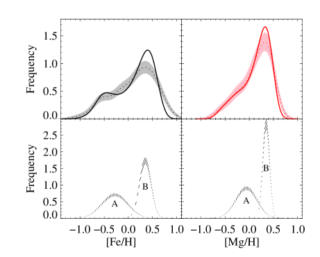
Figure 13: Upper left panel: Smoothed distribution of [Fe/H], as in Fig. 10, with the resulting deconvolved distribution using a constant error (solid line). Upper right panel: Smoothed distribution of [Mg/H], as in Fig. 10 with the resulting deconvolved distribution using a constant error (solid line). Lower left panel: Resulting Gaussian populations in the [Fe/H] distribution. See Table 5 for the parameters of the Gaussians. The error bars represent the uncertainty in the amplitude of the Gaussian populations. Lower right panel: Resulting Gaussian populations in the [Mg/H] distribution.

4.2.2 Gaussian mixture

The metallicity distributions described in Section 5.1 suggest that they may be made up of contributions from different stellar populations. In a first attempt to identify possible sub-structures, we have decomposed the observed [Fe/H] and [Mg/H] distributions into a finite number of Gaussian components. The SEMMUL algorithm, developed by Celeux & Diebolt (1986), was applied. SEMMUL (Stochastic, Estimation, Maximisation, MULtidimensional) is an iterative method for numerically approximating maximum likelihood estimates for incomplete data with a stochastic step to accelerate the convergence. It allows separation of Gaussian components without a priori knowledge of the number of components (only a maximum number is necessary). In addition, it does require defining a set of initial conditions. The algorithm has been modified by Arenou (1993) in order to take observational errors into account, thus the modified version allows to estimate the cosmic dispersion of the population.

SEMMUL has been applied to the 1-dimensional [Fe/H] and [Mg/H] distributions separately, and to the 2-dimensional joint distribution ([Fe/H],[Mg/H]). Thousands of runs were carried out in each case, assuming that the sample is a mixture of 2 or 3 discrete components. In all cases, the algorithm converges to a two-component solution with stable results, dividing the sample in roughly two equal-sized populations.

The resulting two components (that we call A and B) are summarised in Table 5. For each component, the mean chemical composition, the dispersion and the fraction (in percent) of stars in each group, with the corresponding standard errors, are given. The A and B population characteristics are very consistent among the three separations (one-dimensional along [Fe/H] or [Mg/H], or 2-dimensional).

In Sect. 4.1.3 we have argued that the high-metallicity tail of the iron distribution may be biased. In this context, we may wonder whether the mean values and dispersions obtained in the Gaussian decompositions of population B are realistic. The comparison between the estimated mean values ($\rm[Fe/H]=0.32$ and $0.29$, see Table 5) and the median values obtained from the cumulative metallicity distribution (for $\rm[Fe/H]>0$) in Sect.4.1.3 ($\rm[Fe/H]=0.32$ to $0.36$) shows that they are consistent. On the other hand, the obtained cosmic dispersions of population B ($0.11$-$0.12$ dex) could arguably be underestimated. However, according to the same cumulative distribution presented in Sect. 4.1.3, the total metallicity dispersion is about 0.2 dex in this population, and the expected measurement errors are of the same order, which implies that the cosmic dispersion of the population is small, as obtained by our algorithm.

4.2.3 Characterising the two populations

Two populations are clearly identified by the Gaussian separation exercise. The metal-poor component (A) is centred around $\rm[Fe/H]=-0.30$ and $\rm[Mg/H]=-0.06$, with a large dispersion ($\sim 0.3$ dex), while the metal-rich component (B) has similar mean Fe and Mg content ($\rm[Fe/H]=0.32$ and $\rm[Mg/H]=+0.35$) and a very small dispersion (0.11 in [Fe/H] and 0.07 in [Mg/H]).

The dispersion of population B is very small, comparable in fact to the metallicity dispersion of Galactic disc in the solar neighbourhood (or even smaller). The more metal-poor population A is on the contrary quite extended, both in [Fe/H] and in [Mg/H]. This dispersion could in part be due to contamination (see Sect. 2.3) by the thick disc in the inner Galactic regions, that could account for $\sim 10-15\%$ of population A ($5.9\%$ of the total sample). In fact, we will see in the following section that the chemical signature of this population (A) is not distinct from that of the thick disc, and we can therefore not exclude that part of it is made up of thick disc stars, indistinguishable from the bona-fide bulge population by any of our observables.

It is further interesting to note that the two components thus separated are more widely separated in [Fe/H] than in [Mg/H], as reflected by the different mean corresponding [Mg/Fe] ratios (see Sect. 4.3 and Fig. 14), hinting at two physically separated populations. While the metal-poor component A has a clearly defined magnesium overabundance of $\rm[Mg/Fe]\sim 0.24$, the metal-rich component B has a significantly lower $\rm[Mg/Fe]\sim 0.05$, not significantly different than the solar neighbourhood disc magnesium to iron ratio.

We tentatively explain the existence of these bulge populations as the result of different origins. In Babusiaux et al. (2010), we combine the abundances and the kinematics (radial velocities plus proper motions from OGLE-II) and show a significant difference in the kinematics of the metal rich and the metal poor components. The velocity ellipsoid of the metal rich component shows a vertex deviation consistent with what is expected from a population kinematically supporting a bar. The metal poor component on the other hand shows no vertex deviation, consistent with an old spheroidal population. We therefore relate the richest population to a bar-driven pseudo-bulge and the more metal poor one to an old spheroid with a rapid time-scale formation. Similar results have been suggested by Soto et al. (2007) and Zhao et al. (1994), based on kinematics and low resolution metallicities.

Let us note finally that this mixture of populations in Baade’s Window is fully compatible with the variation of the metallicity distribution as a function of Galactic latitude noticed by Zoccali et al. (2008) (from b=$-4$ to $-12^{\circ}$), that we would therefore attribute to the gradual disappearance of the pseudo-bulge component B as one moves away from the Galactic plane, while the old spheroid (A) would dominate out to higher latitudes. The absence of gradients in the inner bulge found by Rich et al. (2007) is also consistent, as this region would be dominated by component B only. We also note that population B also has to be predominantly old (perhaps not surprisingly if disc formation occurs inside out), given that Clarkson et al. (2008) find a pure old population in a field at $\rm b=-2.65^{\circ}$ (i.e. significantly closer to the plane than Baade’s Window).

Table 5: Separation of the sample in two Gaussian components (A and B), with [Fe/H], [Mg/H] or both simultaneously as discriminant variables. ($\rm\sigma_{[Fe/H]}$ and $\rm\sigma_{[Mg/H]}$ are the cosmic dispersion of the population)

	$\rm\overline{[Fe/H]}$	$\rm\sigma_{[Fe/H]}$	$\rm\overline{[Mg/H]}$	$\rm\sigma_{[Mg/H]}$	$\%$
1D-separation along [Fe/H]				$\rm N_{stars}=219$
A	$-0.30{\scriptstyle\pm 0.03}$	$0.25{\scriptstyle\pm 0.01}$			$45{\scriptstyle\pm 3}$
B	$0.32{\scriptstyle\pm 0.01}$	$0.11{\scriptstyle\pm 0.01}$			$55{\scriptstyle\pm 3}$
1D-separation along [Mg/H]				$\rm N_{stars}=162$
A			$-0.06{\scriptstyle\pm 0.02}$	$0.22{\scriptstyle\pm 0.01}$	$49{\scriptstyle\pm 4}$
B			$0.35{\scriptstyle\pm 0.01}$	$0.07{\scriptstyle\pm 0.01}$	$51{\scriptstyle\pm 4}$
2D-separation in ([Fe/H],[Mg/H])				$\rm N_{stars}=162$
A	$-0.27{\scriptstyle\pm 0.03}$	$0.31{\scriptstyle\pm 0.02}$	$-0.04{\scriptstyle\pm 0.03}$	$0.25{\scriptstyle\pm 0.01}$	$53{\scriptstyle\pm 4}$
B	$0.29{\scriptstyle\pm 0.01}$	$0.12{\scriptstyle\pm 0.01}$	$0.36{\scriptstyle\pm 0.01}$	$0.07{\scriptstyle\pm 0.01}$	$47{\scriptstyle\pm 4}$

4.3 The [Mg/Fe] trend in the bulge

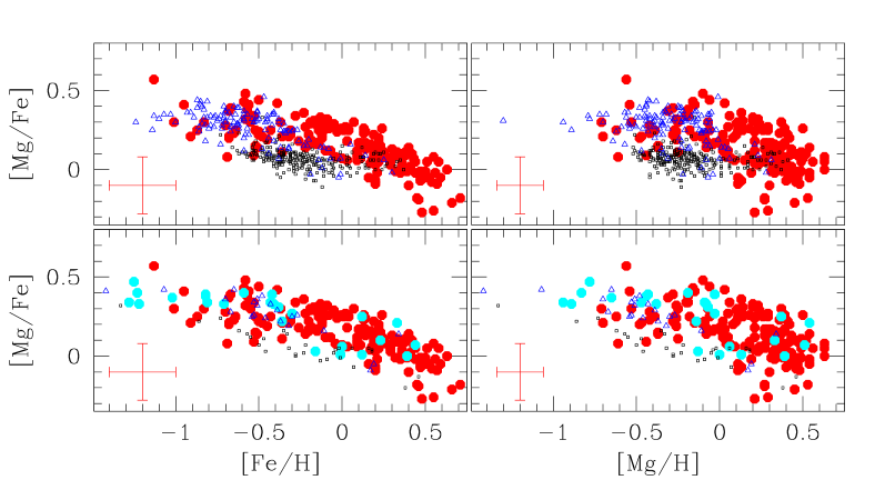
Figure 14: [Mg/Fe] as a function of [Fe/H] (right panel) and [Mg/H] (left panel) for our bulge red clump sample (red points) compared with thick (blue) and thin (black) discs stars. In the two upper panels, the disc reference samples are from the main sequence stars studies of Bensby et al. (2005) (triangles), Reddy et al. (2006) (squares) Fuhrmann (2008) (crosses), whereas the two lower panels show the solar neighborhood disc giants by Alves-Brito et al. (2010), as well as their bulge giants (large filled cyan circles). In the low metallicity range ($\rm[Fe/H]<-0.3$ and $\rm[Mg/H]<0$), the thick disc and the bulge show similar [Mg/Fe] ratios, higher than in thin disc stars.

Our Mg results in terms of [Mg/Fe] against [Fe/H] and [Mg/H] are shown in Fig. 14 (red points). The [Mg/Fe] ratios in the bulge decreases with both [Fe/H] or [Mg/H] from $\rm\sim+0.5$ to near solar values. Comparing our results with the recent optical and IR studies of bulge giants from Rich & Origlia (2005), Fulbright et al. (2007) and Rich et al. (2007) on the common metallicity ranges, we note that the general trend is similar, although our much larger statistics allow us to define the trend with more confidence.

To understand the relation that the bulge bears to the Galactic disc(s), it is interesting to compare the [Mg/Fe] ratios in the bulge sample to the abundance trends found in the Galactic thin and thick discs. In Fig. 14, we plotted the thin (black symbols) and thick (blue symbols) disc stars abundances from the studies of Bensby et al. (2005); Reddy et al. (2006) and Fuhrmann (2008). These studies are based on very careful and thoughrough analysis of large samples of dwarf stars in the solar neighbourhood. As recently pointed out by Meléndez et al. (2008); Alves-Brito et al. (2010), it would be better, for the sake of minimising possible systematics in the abundance analysis, to compare bulge giants with solar neighbourhood thin and thick disc giants observed and analysed in the same conditions. However, from a statistical point of view, the available samples of local giants available for such comparisons is still quite small (Alves-Brito et al., 2010, $\sim$20/30 thick/thin disc stars respectively, ). We therefore decided to stick to a comparison to local disc dwarfs, once a number of verifications were performed: (i) we analysed the [Mg/Fe] of two reference stars, $\mu$Leo and Arcturus ([Mg/Fe]=+0.12 and +0.38), that respectively fall on top of their parent population as derived from local dwarf samples; (ii) Fulbright et al. (2007) analysed a sample of local K giants, and found no difference between the [Mg/Fe] trend derived from these giants and those defined from local dwarfs; (iii) Mishenina et al. (2006) also analysed a large sample of local red clump giants, and reach a similar conclusion for [Mg/Fe]. From these checks, we conclude that it is fair to compare the [Mg/Fe] abundances for the bulge red clump giants presented here to those of local disc(s) dwarfs. In Fig. 14, the two lower panels show that indeed our conclusions would not be altered in any way if comparing our sample to local giants (Alves-Brito et al., 2010). We however caution that in the highest metallicity regime, systematic differences of the order of 0.10-0.15 on the [Mg/Fe] trends are found between different studies of dwarfs stars (for example Reddy et al. (2006) vs. Fuhrmann (2008)), between dwarf and giant stars samples (for example Bensby et al. (2005) vs. Mishenina et al. (2006)) and between different disc giants stars sample (for example Fulbright et al. (2007) vs Mishenina et al. (2006)). This is clearly a domain where abundances have to be taken with caution in general, and even more so when they are derived, as here, from moderate S/N and resolution spectra.

When compared to the local Galactic discs abundances these various bulge samples show some differences depending on the metallicity range:

In the range $\mathit{[Fe/H]\lesssim-0.3}$, the number of stars in the present sample has increased dramatically compared to our previous UVES sample (Fig. 7) and they clearly show [Mg/Fe] ratios similar to those of the thick disc stars for all [Fe/H]. In the same metallicity range, our results differ from those of Fulbright et al. (2007) who found higher [Mg/Fe] values than ours and a [Mg/Fe] trend higher than that of their sample of disc giants. In fact, if we use Arcturus as a reference to insure that the results of Fulbright et al. (2007) are on the same scale as the present work, an offset of $\rm\sim 0.10$ is expected ($\rm[Mg/Fe]_{Fulbright}-[Mg/Fe]_{present}=+0.11$), bringing the [Mg/Fe] of the two studies into agreement.

In the range $\mathit{-0.3\lesssim[Fe/H]\lesssim+0.1}$, the bulge [Mg/Fe] trend from our sample is clearly distinct and higher than that of the thin disc, whatever comparison sample is used. In the same metallicity range, our bulge stars show [Mg/Fe] values on the mean higher than those of the thick disc stars. This confirms, with better statistics our previous results from the UVES sample (Lecureur et al., 2007) as well as the results of Fulbright et al. (2007). Given the residual systematic effect in the [Mg/Fe] determination from GIRAFFE and UVES spectra for the stars in common (see Fig. 8), the difference between thick disc and bulge would be even more pronounced if we adopted the UVES abundances as the reference. However, this difference between bulge and thick disc has to be viewed with caution because of the small number of thick disc stars in this metallicity range, and the still debated thick-disc nature of this high-metallicity tail. Indeed, Bensby et al. (2005, 2007) argue that the thick disc extends at least to solar metallicities and shows a clear decrease of $\rm[\alpha/Fe]$ with increasing iron content for stars with $\rm[Fe/H]\gtrsim-0.3$ denoting an extended star formation period (SNIa enrichment). On the contrary, several authors (Reddy et al., 2006; Fuhrmann, 2008) argue that the thick disc does not extend significantly in this metallicity regime, and that there is no evidence of decreasing $\rm[\alpha/Fe]$ in the thick disc at all.

In the range $\mathit{[Fe/H]\gtrsim+0.1}$, the bulge shows [Mg/Fe] ratios which are similar to those of the local thin disc, solar on the mean, and with a decreasing [Mg/Fe] trend with increasing metallicity. This result confirms, with better statistics, the results found for the oxygen by Meléndez et al. (2008) in the same metallicity regime. On the contrary, our bulge [Mg/Fe] ratios are significantly lower than those of Fulbright et al. (2007), even allowing to shift the latter by $\rm\sim-0.10$ to insure that both studies lie on the same scale. We further note that Fulbright et al. (2007) derived [Mg/Fe] $\rm=+0.02$ for $\mu$Leo, $\rm 0.20$ lower than what we found for this star (Lecureur et al., 2007). At such high metallicities, both Fe and Mg measurements remain quite uncertain which could explain part of the difference between our study and the one of Fulbright et al. (2007). Moreover, the comparison of the bulge and disc trends should be taken with caution in that metallicity regime, since, as pointed out above, systematic differences of the order of 0.10-0.15 are found between the [Mg/Fe] trends at supersolar metallicities between different studies. More specifically, taking as a comparison the local disk sample of giants by Fulbright et al. (2007), we would find that the [Mg/Fe] of the bulge lies above that of the local disk, at variance with the conclusion that is drawn from the comparison to local dwarfs. However, we do not favour this interpretation since Fulbright et al. (2007) also finds $\mu$Leo +0.11 dex lower in [Mg/Fe] than we do.

Very recently, several papers have measured detailed abundances of a few bulge dwarfs from high resolution and high signal to noise ratio spectra obtained during a gravitational microlensing event (Bensby et al., 2010b, 2009b, 2009a; Cohen et al., 2008, 2009; Johnson et al., 2007, 2008). There are in total by now 14 microlensed dwarfs and subgiants analysed in the Galactic bulge (Bensby et al., 2010b), and although the early (2007 and 2008) microlens events yielded a sample of stars almost exclusively metal-rich that was irreconcilable with the MDF of bulge giants (Cohen et al., 2008, 2009; Epstein et al., 2010), the 2009 and 2010 events have uncovered a significant metal-poor population, taming down this conclusion to the point that Bensby et al. (2010b) claims that the two distributions could statistically arise from the same parent population, albeit a rather small probability. The current MDF from these microlensed un-evolved stars is now highly bimodal, with a peak at $\rm[Fe/H]\sim+0.3$ and another one at $\rm[Fe/H]\sim-0.5$ dex. This is very similar to the peaks uncovered by our population separation in the red clump sample. Interestingly, the metal-rich (similar to our population A) and metal-poor (similar to our population B) microlensed stars also have different ages, the latter being a clearly old population, while the former spans a range of ages (2-13 Gyrs). This is again compatible with our suggestion that population B is related to the old bulge while population A is kinematically related to a bar and would be made of a pre-existing disc. Even more interestingly perhaps, we are now in a position to compare the [Mg/Fe] trends in the bulge from dwarf and giants stars: as is our bulge giants, [Mg/Fe] in dwarfs overlays the local thin disc at super-solar metallicities, and the local thick disc at metallicities $[Fe/H]<=-0.3$. The current sample of microlensed giants only contains two stars in the intermediate metallicity range (Bensby et al., 2010b), where we find the bulge to be richer in [Mg/Fe] than both the local thin and thick discs. These two stars seem to trace the upper envelope of the local thick disc. To draw any further conclusion on this metallicity range, more microlensed dwarfs will need to be analysed.

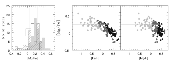
Figure 15: Left panel: [Mg/Fe] distribution for the stars with very high probabilities ($\rm>85$%) to belong to population A (empty histogram) and B (shaded histogram). The two lines show the peaks of these two distributions: 0.05 and 0.25 respectively. The hatched histogram represents the stars with low probabilities to belong to one or the other population. Right panels: [Mg/Fe] as a function of [Fe/H] and [Mg/Fe] for the three groups of stars.

To follow up on our tentative sample separation in two distinct populations we colour-coded in Fig. 15, the stars belonging to the populations A and B as separated in Table 5 along [Mg/H], using the probability with which a star was assigned to its population. All stars with very high probabilities ($>85\%$) to belong to population A are coded in light grey, while those with high probability to be in B are coded in black. Stars that are in dark grey are those with low probabilities to belong to one or the other class. Population A shows high [Mg/Fe] ratios, with a mean of $\rm[Mg/Fe]=0.25$, while population B has lower Mg enhancements, close to solar, as discussed above. The intermediate RC population (those stars that could not be unambiguously classified) has both high and low [Mg/Fe] ratios. In fact, the [Mg/Fe] histogram of this population shows two well defined peaks, one at $+0.25$ and the other at $+0.05$, coinciding precisely with the means for population A and B respectively. It therefore seems that this intermediate population is a mix of stars with the same chemical properties of A or B population, rather than a smooth transition between the two. This is also visible in the run of [Mg/Fe] with metallicity (whether [Fe/H] or [Mg/H], Fig. 15) at intermediate metallicities, where the stars seem to cluster around two discrete [Mg/Fe] values extending the trends of population A and B, rather than follow a smooth decreasing trend. As a result, we argue that population A, that we associate with the old Mg-enhanced bulge, extends up to metallicities of at least [Fe/H]=+0.1 and [Mg/H]=+0.35, and possibly up to [Fe/H]=+0.25 and [Mg/H]=+0.5. Conversely, population B probably extends down to $\rm[Fe/H]\sim[Mg/H]=0.0$, with modest Mg enhancements. This will have an impact on the chemical evolution models that may be appropriate to represent these two populations.

5 Chemical evolution and bulge formation

In this section, with the aim of understanding the formation history and chemical evolution of the galatic bulge, we compared our bulge MD with the results of two recent bulge formation models: the chemical evolution model of Ballero et al. (2007b) and the chemodynamical model of Immeli et al. (2004).

5.1 Comparing to a chemical evolution model of the bulge

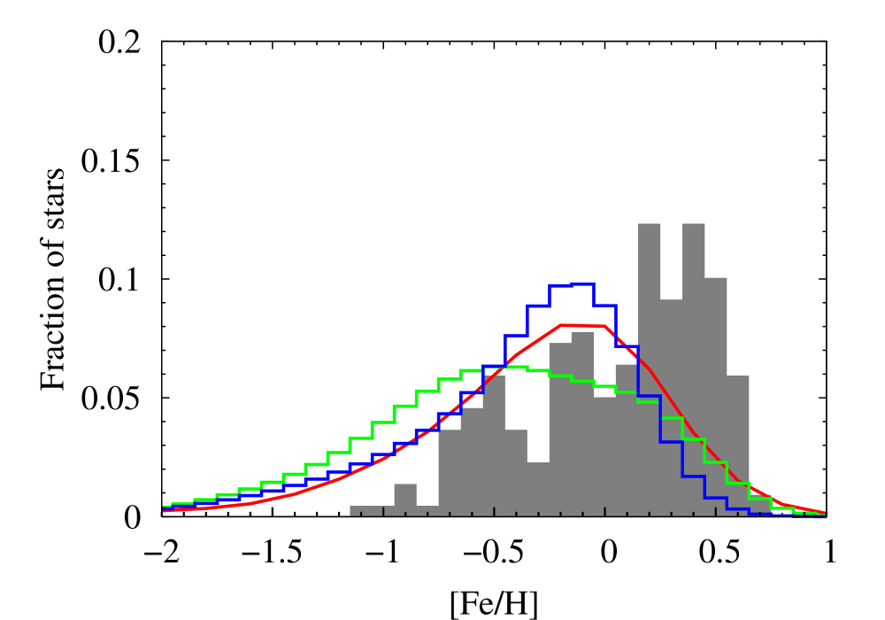
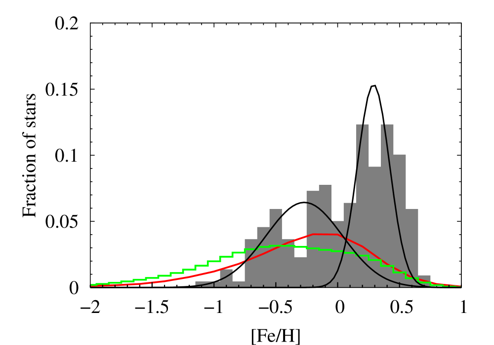
Figure 16: Upper panel. Comparison between the bulge MD predicted by the chemical model of Ballero et al. (2007b) (red line) and by the model of Immeli et al. (2004) (green line for the model B and blue line for the model F ) with the observed MD (shaded histogram). The three model MDs have been convolved with observational errors. Lower panel:. The previous model MDs were normalised to 50% and compared to the MD of the two subpopulations A and B (each of them corresponding to 50% of the total) illustrated here by two Gaussians with position and dispersion according to Tab. 5.

Figure 16 upper panel shows the MD predicted by the model of Ballero et al. (2007b) together with our observed iron MD. For the sake of comparison, the model MD has been convolved with the mean [Fe/H] uncertainties of the observed sample (Fig. 6). By constraining their model parameters from bulge observed abundances ratios and Fe MD, Ballero et al. (2007b) concluded that the bulge formed in a very short time, with a high star formation efficiency ($\rm\mu\simeq 20$ Gyr^-1) and an IMF flatter than in the solar neighbourhood. The MD they predict peaks around solar metallicity and is shifted toward lower metallicities with a more extended metal poor tail with respect to our bulge observed MD. This disagreement was expected given the differences between our bulge MD and the one of Zoccali et al. (2003) and Fulbright et al. (2006) that were used as references by Ballero et al. (2007b). In fact, to predict near solar metallicities MD consistent with high $\rm\alpha$-elements ratios, Ballero et al. (2007b) had to assume an IMF flatter than in the solar neighbourhood but also (see Ballero et al. (2007a)) flatter than the stellar IMF of Kroupa (2001) and the IMF integrated over galaxies of Weidner & Kroupa (2005). According to the tests done by the authors, to shift the predicted MD to more metal-rich (as observed in the present paper), the IMF should be further flattened. However, for IMF slope lower than 0.35, the position of the peak of the predicted MD becomes insensitive to further slope decreases. Moreover, a flatter IMF would in turn lead to predict higher [Mg/Fe] and [O/Fe] ratios than observed. Thus, it seems there does not exist any appropriate set of fundamental parameters for the bulge chemical model of Ballero et al. (2007b) to reproduce both our red clump MD and the [Mg/Fe] (or [O/Fe]) trend observed in the bulge.

On the other hand, if we consider the observed MD as the result of two populations (see Sect. 4.2), it would be more appropriate to compare the MD of Ballero et al. (2007b) (given their bulge chemical model formation hypothesis) with the one associated to the old bulge component. This comparison is illustrated by the Fig. 16 where the old bulge population (A) is modelled by a Gaussian with a mean [Fe/H] of -0.3 and a width of 0.25. With its actual parametrisation, the model of Ballero et al. (2007b) also fails to reproduce the metal-poor population of the bulge. The predicted MD peaks at [Fe/H] values higher than the mean of population A, and is wider than the Gaussian. It underpredicts the fraction of stars in population A at intermediate metallicities ($\rm-0.8<[Fe/H]<-0.1$) and predicts a longer low metallicity tail ($\rm[Fe/H<-0.8$). However, based on the parameter variations presented by Ballero et al. (2007b), we would expect that it should be possible to find a set of parameters that would reproduce both the high [Mg/Fe] and metallicity distribution of population A. In particular, there would not be the need for a flatter IMF in the bulge anymore.

5.2 Comparing to a chemodynamical model

Figure 16 lower panel shows the comparison between our bulge iron MD and the predicted MD from two models (B and F models) of Immeli et al. (2004) convolved with the observational errors. Immeli et al. (2004) investigated different scenarios of bulge, disc and halo populations formation from the evolution of a star-forming disc with a chemodynamical 3D model including initial conditions from $\rm\Lambda CDM$ results and a two phases (gas and stars) interstellar medium. The Galactic bulge is formed in very different way depending on values adopted for the efficiency of energy dissipation of the cold cloud component from which stars form. With a high efficiency of energy dissipation, a massive bulge is formed from the central merging of clumps of stars and gas at relatively early times (model B). On the contrary, with low efficiencies values the instability occurs in the stellar disc at later time forming a stellar bar which evolves and forms a pseudo-bulge (model F).

The two predicted MD are completely different from the observed one. As already explained in the previous section, this was expected for the model B leading to the formation of a massive bulge. However, the B model MD does not agree either with the metal poor component of the observed MD (population A). It peaks around [Fe/H] $\rm=-0.40$, close to the mean of the Gaussian representative of the old bulge but is wider than this population, and overproduces the fraction of metal-poor stars with respect to the actual observed MD.

The observed and model F MDs peak at distinct metallicities ($\rm[Fe/H]\sim+0.3$ and $\rm\sim-0.2$ for the observed and model F respectively), but have a quite similar global shape. Indeed, if we artificially shift the model F MD of $\rm+0.5$, the differences between the two MD are less pronounced, even if differences in the lowest and highest metallicities regimes persist. The shifted F MD would overestimate the number of stars at low metallicities ($\rm[Fe/H]<-0.8$ dex) and underestimate the number of stars at high metallicities ($\rm[Fe/H]>0.1$), in addition to showing a more progressive decrease of the number of stars than observed at high metallicities. We will come back in Sect.5.3 on these differences. However, if we believe the scenario of Immeli et al. (2004) for the bulge formation (model F), we can not explain why such a large shift ($\rm+0.5$) in mean metallicity would be required. Uncertainties in the stellar yields adopted can not explain such a large difference. To obtain such metal-rich stars, we would suggest that the gas forming the stellar disc (from which the pseudo-bulge is formed) could have been previously enriched. Several factors could have contributed to the enrichment of this gas, but one possibility could be enriched gas left over (or blown out) from the old bulge formation.

5.3 An attempt at modelling the two populations

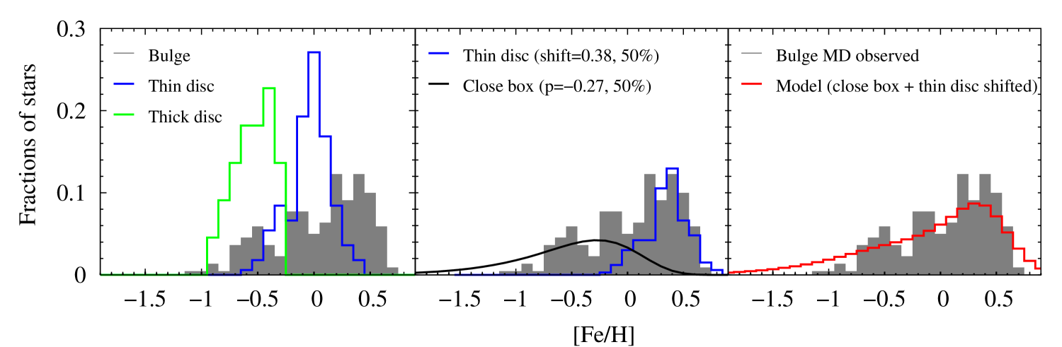
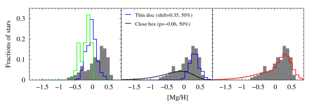
Figure 17: The left panels show the comparison of the [Fe/H] MD (upper) and [Mg/H] MD (lower) with the thin (blue) and thick (green) discs MD in the solar neighbourhood from the study of Fuhrmann (2008). The distinction between the three populations is clear from their [Fe/H] and [Mg/H] MD in their global shapes, their mean values and the metallicity range they cover. In the middle panels the bulge [Mg/H] and [Fe/H] MD are compared to a close box model with a yield $\rm p=-0.27$ and $-0.06$ for Fe and Mg respectively (black line) and to the previous thin disc MD shifted by $+0.35$ (blue) according to the results of the Gaussian separation (see Sect. 4.2 and Table 5). The combination of these two MD convolved are compared to the observed ones (right panels) for Fe (upper) and Mg (lower). For both elements, the model MD shows a very good agreement with the observed one. A small difference (compared to the relative errors) exists on the high metallicities tails: the high metallicity tail of the Mg and Fe MD decrease more sharply than the model distributions.

Without any satisfactory bulge formation model that could explain the observed MD, we tried to build a simple modelling of the two populations according to their respective formation mechanism suggested by the results of Babusiaux et al. (2010). The metal-poor population has kinematics that show no influence of the Galactic bar, and in addition, we find it to be enriched in [Mg/Fe], which reinforces out interpretation of this population as an old spheroid with a rapid time-scale formation. To produce the chemical evolution of this population, we used a simple closed-box model. This model predicts that the metallicity (Z) distribution function (MDF) follows the relation $\rm f(Z)=p^{-1}e^{-Z/p}$ where p is the stellar yield given by $\rm p=<Z>$. For p, we adopted the mean values of the Gaussian associated to the metal old population: $-0.06$ and $-0.30$ [Mg/H] and [Fe/H] respectively. The resulting [Fe/H] and [Mg/H] metallicities distribution (scaled to 50% of the total population to represent population A only)) are compared to the red clump ones on Fig. 17 (middle panels).

As explained in Babusiaux et al. (2010), the kinematical characteristics of the richest population suggest that it is under the influence of a bar. Adding to this the fact that [Mg/Fe] in this population is near solar, we suggest a formation over a long time scale through the evolution of the bar, itself originating in disc instability. Within this scenario, population B stars observed in Baade’s window would have been ejected from the inner regions of the Galactic disc. We then expect the chemical composition of these stars to be the same as the one of the old inner disc at the time when the bar formed. However, as already mentioned, little is known about the inner regions of the Galactic disc. A metallicity gradient has been observed in young populations (OB stars, HII regions, Cepheids) but observational constrains of the old populations are missing. To reproduce the MD of the richest population, we adopted the MD of the solar neighbourhood from Fuhrmann (2008), scaled it to 50 % of the total sample (to represent population B only), and shifted toward higher metallicity in order to reproduce the possible gradient in the Galactic disc. The Fuhrmann (2008) Fe and Mg metallicity distributions are symmetric around mean values of $\rm[Fe/H]=-0.03\pm 0.01$ and $\rm[Mg/H]=0.00\pm 0.01$, and narrower than the bulge MD (see Fig. 17, left panels). On the middle panels of Fig. 17, we plot the Fuhrmann (2008) Fe and Mg MD scaled to 50 % of the total bulge population, and shifted by $+0.35$ for both Fe and Mg, so that their mean values coincide with those of the corresponding Gaussian components. These Mg and Fe MD shifted disc components seem to be good candidates to reproduce the observed bulge metal rich component. The main difference (more pronounced for Fe than for Mg MD) appears at very high metallicities, where the observed bulge MD shows a sharper cutoff than in that of the shifted disc. Assuming that this mock disc would originate in the very inner parts of the Galactic disc, around 8 kpc from the Sun, the shifts applied to the local thin disc MD of Fuhrmann (2008) correspond to gradients of $\rm-0.047dex.kpc^{-1}$ for Fe and $\rm-0.043dex.kpc^{-1}$ for Mg. These gradients are similar to the gradients that have been observed in the youngest populations of the inner and outer disc (Daflon & Cunha, 2004). However, in our case we are not interested in the value of the present day gradient in the Galactic disc but rather what it was in the past, when the stars that we now see in the pseudo-bulge would have formed. Recent observations of planetary nebulae and open clusters in the Galatic disc (see Maciel & Costa, 2009, and references therein) suggest a flattening of the metallicity gradients with time which is not consistent with the gradient we derived. The chemical evolution models of the disc assuming an inside-out formation scenario (Cescutti et al., 2007; Chiappini et al., 2001) predict gradients at the present day whose values agree with the observations of young and intermediate-age populations of the disc. But, these models also predict that the gradients were flatter at in the past. Cescutti et al. (2007, private communication) found that 9 Gyrs ago, gradients were only of $\rm-0.014dex.kpc^{-1}$ for Fe and of $\rm-0.017dex.kpc^{-1}$ (in the range of galactocentric distances from 4 to 14 kpc). These values, if extended would also be inconsistent with our findings.

On Fig. 17, we plotted the sum of the two modelled MD associated to the metal poor and metal rich components. The MD predicted by the Simple model have been convolved with the observed mean uncertainties for our sample (Fig. 6). The internal errors of the Fuhrmann (2008) data being much lower than the observed one, the disc MD have also been convolved with a Gaussian with $\rm\sigma=0.18$ for Fe and $\rm\sigma=0.12$ for Mg. For both elements, the combined MD show a fairly good agreement with the observed ones. The main differences concern the metal poor tail and the richest part of the distributions.

In the very metal poor regime ([Fe/H] $\rm<-0.7$ and [Mg/Fe] $\rm<-0.5$), the closed box model predicts more stars with respect to what is observed. The same lack is observed in the solar neighbourhood thin disc and is well known as the G dwarfs problem. For our red clump sample, it is not likely that this difference could come from a selection effect, at least down to $\rm[Fe/H]=-1.5$ (see Sect. 2.3). As for the local disc, the G dwarf problem in the bulge could be partly or totally solved by including an infall of primordial gas in chemical evolution models. Additional observations of the bulge in the very metal poor regime would also help to answer this question.

At higher metallicities, the observed MDs show a peak more pronounced and a sharper decrease than the shifted MD of the thin disc. These differences are quasi insensitive to changes up to 0.05 dex on the adopted shifts for Mg and Fe but could be reduced by decreasing the adopted width of the convolution (reproducing observed errors) down to an unrealistic level of 0.10. In Sect. 4.1.3, we have argued that the high-metallicity tail of the iron MD may be biased at the highest metallicity stars, in a direction that is not yet very clear: experiments with synthetic spectra suggest that we may overestimate the metallicities of super-solar metallicity stars by up to $0.15$ dex, whereas the estimated errors and sharpness of the decrease of the metal-rich tail may be read as a hint that the highest metallicities are underestimated.

6 Summary and conclusions

We have analysed a sample of 219 bulge red clump stars in Baade’s window from R=20000 resolution spectra obtained with FLAMES/GIRAFFE at the VLT. This sample has been selected based on the location of stars in the Colour-Magnitude Diagram, in order to minimise the contamination by other Galactic components ($\rm<10$ % from the latest population synthesis Besançon model (Robin et al., 2003; Picaud & Robin, 2004), and hence is a good tracer of the bulge metallicity distribution (MD) in the Baade’s window.

For these stars, with an automatic procedure, we have derived the stellar parameters and Fe abundances using an iron linelist established differentially to $\mu$Leo and for a subsample of 162 stars (built by excluding stars with high uncertainties on [Fe/H]), we also derived the Mg abundances with spectral synthesis around the Mg I triplet at $\rm\lambda$ 6319 Å.

The Fe and Mg metallicity distributions are both asymmetric, with mean values of $\rm+0.05\pm 0.03$ and $\rm+0.14\pm 0.03$, and median values of $\rm 0.16$ and $\rm 0.21$ respectively. They show a small proportion of stars at low metallicities ($\rm<3$ % with $\rm[Fe/H]<-0.7$ or $\rm[Mg/H]<-0.4$), only extending down to $\rm[Fe/H]=-1.1$ or $\rm[Mg/H]=-0.7$. The iron MD is not well reproduced by the predictions of the chemical models of the bulge available in the literature (Ballero et al., 2007b, a), neither by models adding dynamical aspects to chemical prescriptions such as the one of (Immeli et al., 2004).

The decomposition of the observed Fe and Mg MDs into Gaussian components has revealed the presence of two populations of equal sizes (50% each): a metal-poor component centred around [Fe/H] $\rm=-0.30$ and [Mg/H] $\rm=-0.06$ with a large dispersion and a narrow metal-rich component centred around $\rm[Fe/H]=0.32$ and $\rm[Mg/H]=+0.35$. The metal poor component shows high [Mg/Fe] ratios (around 0.3) whereas stars in the metal rich component are found to have near solar ratios. Babusiaux et al. (2010) also found kinematical differences between the two components: the metal poor component shows kinematics compatible with an old spheroid whereas the metal rich component is consistent with a population supporting a bar. In view of their chemical and kinematical properties, we suggest different formation scenarios for the two populations: a rapid formation timescale as an old spheroid for the metal poor component (old bulge) and for the metal rich component, a formation over a longer time scale driven by the evolution of the bar (pseudo-bulge). This latter component represents  50% of the total Baade’s Window population, and is of old age (Clarkson et al., 2008, as indicated by deep colour-magnitude diagrams, see e.g.), indicating that a fairly massive disc was present some 10Gyr ago, which may turn out to be a strong constraint on models of disc formation. It is suggestive that the local thick disc and old bulge display the same [Mg/Fe] enhancement, pointing at similarly rapid star formation process. At this point, it is however not possible to constrain further the relationship that the old bulge bears with the thick disc, both because of lack of constraints on the central parts of the thick disc (both chemistry and kinematics), and because our bulge sample being located on the minor axis, we have a very poor constraint on rotation and the disky nature of this component can therefore not be probed from our data. We however not that in their recent study, Bensby et al. (2010a) finds that the inner parts of the thick disc is chemically very similar to that in the solar neighbourhood, lending strong support to the idea that the metal-poor bulge is indeed chemically related to the thick disc. We also note that the numerous metal-rich globular clusters of the Milky Way, that are concentrated towards the inner parts of the galaxy, would be classified as old bulge in our scheme (see e.g. Bica et al. 2006 that show clusters with $\rm[Fe/H]<-0.75$ are confined within 2kpc of the centre). It is interesting to note that the most metal-rich globular cluster known so far is NGC 6528 (Ortolani et al. 2007), with $\rm[Fe/H]=-0.2$ (Zoccali et al. 2004), therefore within the metal-poor bulge component identified here.

Guided by these results, we built a simple model combining two components. We used a simple closed box model to predict the metal poor population contribution, whereas we represented the metal rich population by the MD of the local thin disc (Fuhrmann, 2008), shifted to the centre of the corresponding metal rich population. The resulting combined MD shows a good agreement with the red clump one on the whole metallicity range except for the very metal poor and very metal rich regimes, where more stars are predicted than observed. The bulge (old bulge) thus seems to exhibit the G dwarfs problem. The shift we had to apply to the local thin disc MD to fit the metal-rich population is however quite large (although not impossible) when compared with plausible values of the gradients in the early Galactic disc. One possibility could be that these stars were born in a pre-enriched environment, enriched by the remnant of the old bulge.

The scenario(s) proposed here should now be turned into proper modelling (chemical and kinematical) of the bulge that would include two formations events (linked or not), to evaluate their viability. Expanding similar combined chemical and kinematical studies of large samples towards various directions in the Galactic bulge would also be of great help for answering these questions. In particular, probing the bulge at lower latitudes and along longitude should trace the relative importance of the metal-rich and metal-poor populations and definitively establish their proposed different (kinematical and chemical) nature as an old bulge and pseudo-bulge. Because these regions are much more heavily obscured than Baade’s window, this kind of observations will have to be carried out in the infrared. Finally, we note that our group has undertaken similar red clump observations of the inner parts of the Galactic disc that are expected to shed new light on the true relation between the disc and the pseudo-bulge.