Analysis of the Incircle predicate for the Euclidean
Voronoi diagram of axes-aligned line segments

Abstract

In this paper we study the most-demanding predicate for computing the Euclidean Voronoi diagram of axes-aligned line segments, namely the Incircle predicate. Our contribution is two-fold: firstly, we describe, in algorithmic terms, how to compute the Incircle predicate for axes-aligned line segments, and secondly we compute its algebraic degree. Our primary aim is to minimize the algebraic degree, while, at the same time, taking into account the amount of operations needed to compute our predicate of interest.

In our predicate analysis we show that the Incircle predicate can be answered by evaluating the signs of algebraic expressions of degree at most 6; this is half the algebraic degree we get when we evaluate the Incircle predicate using the current state-of-the-art approach. In the most demanding cases of our predicate evaluation, we reduce the problem of answering the Incircle predicate to the problem of computing the sign of the value of a linear polynomial (in one variable), when evaluated at a known specific root of a quadratic polynomial (again in one variable). Another important aspect of our approach is that, from a geometric point of view, we answer the most difficult case of the predicate via implicitly performing point locations on an appropriately defined subdivision of the place induced by the Voronoi circle implicated in the Incircle predicate.

Key words: Incircle predicate, Euclidean Voronoi diagram, line segments, axes-aligned

1 Introduction

The Euclidean Voronoi diagrams of a set of line segments is one of the most well studied structures in computational geometry. There are numerous algorithms for its computation [6, 16, 18, 24, 8, 1, 17]. These include worst-case optimal algorithms that use different algorithmic paradigms, such as the divide-and-conquer paradigm [24] or the sweep-line paradigm [8]. An interesting and efficient class of algorithms rely on the randomized incremental construction of the Voronoi diagram [1, 17]. From the implementation point of view, there are algorithms that assume that numerical computations are performed exactly [22, 14], i.e., they follow the Exact Geometric Computation (EGC) paradigm [25], as well as algorithms that use floating-point arithmetic [12, 23, 11]; the latter class of algorithms does not guarantee exactness, but rather topological correctness, meaning that the output of the algorithm has the correct topology of a Voronoi diagram. In terms of applications, these include computer graphics, pattern recognition, mesh generation, NC machining and geographical information systems (GIS) — see [16, 18, 3, 11, 9], and the references therein.

Efficient and exact predicate evaluation in geometric algorithms is of vital importance. It has to be fast for the algorithm to be efficient. It has to be complete in the sense that it has to cover all degenerate cases, which, despite that fact that they are “degenerate” from the theoretical/analysis point-of-view, they are commonplace in real world input. In the EGC paradigm context, exactness is the bare minimum that is required in order to guarantee the correctness of the algorithm. The efficiency of predicates is typically measured in terms of the algebraic degree of the expressions (in the input parameters) that are computed during the predicate evaluation, as well as the number (and possibly type) of arithmetic operations involved. The goal is not only to minimize the number of operations, but also to minimize the algebraic degree of the predicates, since it is the algebraic degree that determines the precision required for exact arithmetic. Degree-driven approaches for either the evaluation of predicates, or the design of the algorithm as a whole, has become an important question in algorithm/predicate design over the past few years [4, 19, 2, 5, 15, 7, 20].

In this paper we are interested in the most demanding predicate of the Euclidean Voronoi diagram of axes-aligned line segments. Axes-aligned line segments, or line segments forming a 45-degree angle with respect to the axes, are typical input instances in various applications, such as VLSI design [21, 10]. However, although the predicates for the Euclidean Voronoi diagram of line segments have already been studied [4], the predicates for axes-aligned or ortho-45^∘ input instances have not been studied in detail in the Euclidean setting. In the sections that follow, we analyze the Incircle predicate in this setting: given three sites $S_{1}$, $S_{2}$ and $S_{3}$, such that the Voronoi circle $V(S_{1},S_{2},S_{3})$ exists, and a query object $O$, we seek to determine if $O$ intersects the disk $D$ bounded by $V(S_{1},S_{2},S_{3})$, touches $D$ or is completely disjoint from $D$. In our context $S_{1}$, $S_{2}$, $S_{3}$ and $O$ are either points or axes-aligned (open) line segments. Our aim is to minimize the algebraic degree of the expressions involved in evaluating the Incircle predicate. We show that we can answer the Incircle predicate using polynomial expressions in the input quantities whose algebraic degree is at most 6. This is to be compared: (1) against the generic bound on the maximum algebraic degree needed to compute the Incircle predicate, when we impose no restriction on the geometry of the line segments, which is 40 [4], and (2) against the specialization/simplification of the approach in [4], when we consider axes-aligned line segments. With respect to the latter case, our algebraic degrees are never worse, while in the most demanding case we have reduced the degree by a factor of two (see also Table 1).

The rest of our paper is structured as follows. In Section 2 we give some definitions, compare our approach to that in [4], and detail some of the tools that we use in the Incircle predicate analysis. In Sections 3-7 we describe how we evaluate the incircle predicate for different configurations of the sites $S_{1}$, $S_{2}$, $S_{3}$ and $O$. In Section 8 we detail plans for future work.

2 Definitions and preliminaries

Given three sites $S_{1}$, $S_{2}$, and $S_{3}$ we denote their Voronoi circle by $V(S_{1},S_{2},S_{3})$ (if it exists). There are at most two Voronoi circles defined by the triplet $(S_{1},S_{2},S_{3})$; the notation $V(S_{1},S_{2},S_{3})$ refers to the Voronoi circle that “discovers” the sites $S_{1}$, $S_{2}$ and $S_{3}$ in that (cyclic) order, when we walk on the circle’s boundary in the counterclockwise sense. Given a fourth object $O$, which we call the query object, the Incircle predicate $\textsf{Incircle}(S_{1},S_{2},S_{3},O)$ determines the relative position $O$ with respect to the disk $D$ bounded by $V(S_{1},S_{2},S_{3})$. The predicate is positive if $O$ does not intersect $D$, zero if $O$ touches the boundary but not the interior of $D$, and negative of the intersection of $O$ with the interior of $D$ is non-empty.

The Voronoi circle of three sites does not always exist. In this paper, however, we assume that the Incircle predicate is called during the execution of an incremental algorithm for computing the Euclidean Voronoi diagram of line segments, and thus the first three sites are always sites related to a Voronoi vertex in the diagram. Note that the value of the Incircle predicate does not change when we circularly rotate the first three arguments. In that respect, there are only four possible distinct configurations for the type of the Voronoi circle: $PPP$, $PPS$, $PSS$ and $SSS$, where $P$ stands for point and $S$ stands for segment. For example, a Voronoi circle of $PSS$ type goes through a point and is tangent to two segments. This gives eight possible configurations for the Incircle predicate, two per Voronoi circle type.

The predicates for the Euclidean Voronoi diagram of line segments, in the context of an incremental construction of the diagram, have already been studied by Burnikel [4]. According to Burnikel’s analysis the most demanding predicate is the Incircle predicate: assuming that the input is either rational points, or segments described by their endpoints as rational points, Burnikel shows that the Incircle predicate can be evaluated using polynomial expressions in the input quantities, whose algebraic degree is at most 40; this happens when the Voronoi circle is of $SSS$ type and the query object is a segment (see also the line dubbed “General [4]” in Table 1). Considering Burnikel’s approach for the case of axes-aligned line segments, and performing the appropriate simplifications in his calculations, we arrive at a new set of algebraic degrees for the various configurations of the Incircle predicate (see line dubbed “Axes-aligned [4]” in Table 1); now the most demanding case the is $PPS$ case, which gives algebraic degree 8 and 12, when the query object is a point and a segment, respectively.

	$PPPP$	$PPSP$	$PSSP$	$SSSP$
General [4]	4	12	16	32
Axes-aligned [4]	4	8	4	2
Axes-aligned [this paper]	4	6	4	2

	$PPPS$	$PPSS$	$PSSS$	$SSSS$
General [4]	8	24	32	40
Axes-aligned [4]	6	12	4	2
Axes-aligned [this paper]	6	6	4	2

Table 1: Maximum algebraic degrees for the eight types of the Incircle predicate according to: [4] for the general and the axes-aligned segments case, and this paper. Top/Bottom table: the query object is a point/segment.

In Sections 3-7 we analyze, in more or less detail, all eight possible configurations for the Incircle predicate, and show how we can reduce the algebraic degrees for the $PPS$ case from 8 and 12 to 6. This is done by means of three key ingredients: (1) we formulate the Incircle predicate as an algebraic problem of the following form: we compute a linear polynomial $L(x)=l_{1}x+l_{0}$ and a quadratic polynomial $Q(x)=q_{2}x^{2}+q_{1}x+q_{0}$, such that the result of the Incircle predicate is the sign of $L(x)$ evaluated at a specific root of $Q(x)$, (2) for the $PPS$ and $PSS$ cases, we express the Incircle predicate as a difference of distances, instead of as a difference of squares of distances, and (3) we reduce the $PPSP$ case to the $PPPS$ case. Regarding the first ingredient, we describe in the following subsection how we can do better than finding the appropriate root of $Q(x)$ and substitute it in $L(x)$ (this is essentially what is done in [4]). Regarding the second and third ingredients we postpone the discussion until the corresponding sections. There is one final tool that we will be very useful in order to simplify our analysis: in order to reduce our case analysis we make extensive use of the reflection transformation through the line $y=x$; see Subsection 2.2 for the details.

2.1 Evaluation of the sign of $L(x)=l_{1}x+l_{0}$ at a specific root of $Q(x)=q_{2}x^{2}+q_{1}x+q_{0}$

Let $L(x)=l_{1}x+l_{0}$ and $Q(x)=q_{2}x^{2}+q_{1}x+q_{0}$ be a linear and a quadratic polynomial, respectively, such that $Q(x)$ has non-negative discriminant. Let the algebraic degrees of $l_{1}$, $l_{2}$, $q_{2}$, $q_{1}$ and $q_{0}$ be $\delta_{l}$, $\delta_{l}+1$, $\delta_{q}$, $\delta_{q}+1$, and $\delta_{q}+2$, respectively. We are interested in the sign of $L(r)$, where $r$ is one of the two roots $x_{1}\leq{}x_{2}$ of $Q(x)$. In our analysis below we will assume, without loss of generality that $l_{1},q_{2}>0$.

The obvious approach is to solve for $r$ and substitute into the equation of $L(x)$. Let $\Delta_{Q}=q_{1}^{2}-4q_{2}q_{0}$ be the discriminant of $Q(x)$. Then $r=(-q_{1}\pm\sqrt{\Delta_{Q}})/(2q_{2})$, which in turn yields $L(r)=(l_{1}q_{1}+2l_{0}q_{2}\pm\sqrt{\Delta_{Q}})/(2q_{2})$. Computing the sign of $L(r)$ is dominated, with respect to the algebraic degree of the quantities involved, by the computation of the sign of $l_{1}q_{1}+2l_{0}q_{2}\pm{}l_{1}\sqrt{\Delta_{Q}}$. Evaluating the sign of this quantity amounts to evaluating the sign of $(l_{1}q_{1}+2l_{0}q_{2})^{2}-l_{1}^{2}\Delta_{Q}$, which is of algebraic degree $2(\delta_{l}+\delta_{q}+1)$.

Observe now that evaluating the sign of $L(r)$ is equivalent to evaluating the sign of $Q(x^{\star})$, and possibly the sign of $Q^{\prime}(x^{\star})$, where $x^{\star}=-\frac{l_{0}}{l_{1}}$ stands for the root of $L(x)$. Indeed, if $Q(x^{\star})<0$, we immediately know that $L(r)<0$ if $r\equiv{}x_{1}$, or that $L(r)>0$ if $r\equiv{}x_{2}$. If $Q(x^{\star})>0$, we need to additionally evaluate the sign of $Q^{\prime}(x^{\star})=2q_{2}x^{\star}+q_{1}$. If $Q^{\prime}(x^{\star})<0$, we know that $x^{\star}<x_{1},x_{2}$, which implies that $L(r)>0$, whereas if $Q^{\prime}(x^{\star})>0$, we have $x^{\star}>x_{1},x_{2}$, which gives $L(r)<0$. Finally, if $Q(x^{\star})=0$, we still need to evaluate the sign of $Q^{\prime}(x^{\star})$. If $Q^{\prime}(x^{\star})<0$, then $x^{\star}\equiv{}x_{1}$, and thus $L(r)=0$ if $r\equiv{}x_{1}$, and $L(r)>0$ if $r\equiv{}x_{2}$. Similarly, if $Q^{\prime}(x^{\star})>0$, then $x^{\star}\equiv{}x_{2}$, and thus $L(r)<0$ if $r\equiv{}x_{1}$, and $L(r)=0$ if $r\equiv{}x_{2}$. There is one last case to consider: $Q^{\prime}(x^{\star})=0$. Given that $Q(x^{\star})=0$, this can happen only if $x_{1}=x_{2}=x^{\star}$, in which case we deduce $L(r)=0$. Since $Q(x^{\star})=(l_{1}^{2}q_{0}-l_{1}q_{1}l_{0}+q_{2}l_{0}^{2})/l_{1}^{2}$, evaluating the sign of $Q(x^{\star})$ means evaluating the sign of an algebraic expression of degree $2\delta_{l}+\delta_{q}+2$. Moreover, $Q^{\prime}(x^{\star})=(l_{1}q_{1}-2q_{2}l_{0})/l_{1}$; hence, evaluating the sign of $Q^{\prime}(x^{\star})$ reduces to evaluating the signs of $l_{1}q_{1}-2q_{2}l_{0}$ and $l_{1}$, the degrees of which are $\delta_{l}+\delta_{q}+1$ and $\delta_{l}$, respectively.

Notice that the latter among the two approaches described above is never worse than the first one; in fact, if $\delta_{q}>0$ it gives a lower maximum algebraic degree. We summarize this observation in the following lemma.

Lemma 1.

Let $L(x)=l_{1}x+l_{0}$, $l_{1}\neq{}0$, and $Q(x)=q_{2}x^{2}+q_{1}x+q_{0}$, $q_{2}\neq{}0$, be a linear and quadratic polynomial, respectively, such that the discriminant of $Q(x)$ is non-negative. If the algebraic degrees of $l_{1}$, $l_{2}$, $q_{2}$, $q_{1}$ and $q_{0}$ be $\delta_{l}$, $\delta_{l}+1$, $\delta_{q}$, $\delta_{q}+1$, and $\delta_{q}+2$, respectively, then we can evaluate the sign of $L(r)$, where $r$ is a specific root of $Q(x)$, using expressions of maximum algebraic degree $2\delta_{l}+\delta_{q}+2$.

2.2 Reflection transformation

Let $\mathcal{R}:\mathbb{E}^{2}\rightarrow\mathbb{E}^{2}$ denote the reflection transformation through the line $y=x$. $\mathcal{R}$ maps a point $(x,y)\in\mathbb{E}^{2}$ to the point $(y,x)\in\mathbb{E}^{2}$. The reflection transformation preserves circles and line segments and is inclusion preserving. This immediately implies that, given a Voronoi circle $V(S_{1},S_{2},S_{3})$ defined by three sites $S_{1}$, $S_{2}$ and $S_{3}$, and a query point $Q$, $Q$ lies inside, on, or outside the Voronoi circle $V(S_{1},S_{2},S_{3})$ if and only if $\mathcal{R}(Q)$ lies inside, on, or outside the Voronoi circle $V(\mathcal{R}(S_{2}),\mathcal{R}(S_{1}),\mathcal{R}(S_{3}))$ (cf. Fig. 1 for the case where $S_{1}$ and $S_{2}$ are points and $S_{3}$ is a segment). Hence, $\textsf{Incircle}(S_{1},S_{2},S_{3},Q)=\textsf{Incircle}(\mathcal{R}(S_{2}),\mathcal{R}(S_{1}),\mathcal{R}(S_{3}),\mathcal{R}(Q))$. Notice that reflection reverses the orientation of a circle, which is why we consider the Voronoi circle $V(\mathcal{R}(S_{2}),\mathcal{R}(S_{1}),\mathcal{R}(S_{3}))$ instead of the Voronoi circle $V(\mathcal{R}(S_{1}),\mathcal{R}(S_{2}),\mathcal{R}(S_{3}))$. The same principle applies in the case where the query object is a line segment $QS$: $\textsf{Incircle}(S_{1},S_{2},S_{3},QS)=\textsf{Incircle}(\mathcal{R}(S_{2}),\mathcal{R}(S_{1}),\mathcal{R}(S_{3}),\mathcal{R}(QS))$.

As a final note, the reflection transformation $\mathcal{R}$ maps an $x$-axis parallel segment to a $y$-axis parallel segment, and vice versa. This property will be used, in the sections that follow, to reduce the analysis and computation of the Incircle predicate, where one of the $S_{i}$’s is $y$-axis parallel, to the case where one of the $S_{i}$’s is $x$-axis parallel.

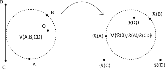
Figure 1: $\textsf{Incircle}(A,B,CD,Q)$ is equivalent to $\textsf{Incircle}(\mathcal{R}(B),\mathcal{R}(A),\mathcal{R}(CD),\mathcal{R}(Q))$, where $\mathcal{R}$ stands for the image of $I$ under the reflection transformation through the line $y=x$.

3 The $PPP$ case

As of this section, we discuss and analyze the Incircle predicate for each of the four possible configurations for the Voronoi circle. We start with the case where the Voronoi circle is defined by three points $A$, $B$ and $C$.

3.1 The query object is a point

This is the well known Incircle predicate for four points $A$, $B$, $C$ and $Q$, where $Q$ is the query point, and it amounts to the computation of the sign of the determinant

$$\textsf{Incircle}(A,B,C,Q)=\begin{vmatrix}1&x_{A}&y_{A}&x_{A}^{2}+y_{A}^{2}\\ 1&x_{B}&y_{B}&x_{B}^{2}+y_{B}^{2}\\ 1&x_{C}&y_{C}&x_{C}^{2}+y_{C}^{2}\\ 1&x_{Q}&y_{Q}&x_{Q}^{2}+y_{Q}^{2}\end{vmatrix}.$$

Its algebraic degree is clearly 4.

3.2 The query object is a segment

Let $QS$ be the query segment. In this case, we must first check that relative position of $Q$ and $S$ with respect to $V(A,B,C)$ using $\textsf{Incircle}(A,B,C,I)$, $I\in\{Q,S\}$. If at least one of $Q$ and $S$ lies inside $V(A,B,C)$, we clearly have $\textsf{Incircle}(A,B,C,QS)<0$.

Otherwise, we have to examine if the segment $QS$ intersects with $V(A,B,C)$. This is equivalent to point-locating the points $Q$ and $S$ in the arrangement of the lines $y=y_{min}$, $y=y_{max}$ and $x=x_{K}$ if $QS$ is $x$-axis parallel or, $x=x_{min}$, $x=x_{max}$ and $y=y_{K}$ if $QS$ is $y$-axis parallel, where $x_{min}$, $x_{max}$ (resp., $y_{min}$ ,$y_{max}$) are the extremal points of $V(A,B,C)$ in the direction of the $x$-axis (resp., $y$-axis). In fact, the case where the segment $QS$ is $y$-axis parallel can be reduced to the case where the query segment is $x$-axis parallel by noting that $\textsf{Incircle}(A,B,C,QS)=\textsf{Incircle}(\mathcal{R}(B),\mathcal{R}(A),\mathcal{R}(C),\mathcal{R}(QS))$ (see Section 2.2). We will therefore restrict our analysis to the case where $QS$ is $x$-axis parallel.

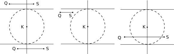
Figure 2: Relative positions of the $x$-axis aligned query segment $QS$ with respect to the lines $x=x_{K}$, $y=y_{min}$, $y=y_{max}$.

We first determine if $Q$ lies outside the band delimited by the lines $y=y_{min}$ and $y=y_{max}$; in this case we immediately get $\textsf{Incircle}(A,B,C,QS)>0$. Otherwise, if $Q$ lies inside the band (resp., $Q$ lies on either $y=y_{min}$ or $y=y_{max}$), we check the relative positions of $Q$ and $S$ against the line $x=x_{K}$; the segment $QS$ intersects (resp., is tangent to) $V(A,B,C)$ if and only if $Q$ and $S$ lie on different sides of the line $x=x_{K}$.

In order to determine the relative position of $Q$ with respect to the lines $y=y_{min}$ and $y=y_{max}$, we will evaluate a quadratic $y$-polynomial that vanishes at $y_{min}$ and $y_{max}$: let $T(y)=t_{2}y^{2}+t_{1}y+t_{0}$ be this polynomial. Having computed this polynomial, $y_{Q}\in(y_{min},y_{max})$ if and only if $sign(T(y_{Q}))=-sign(t_{2})$, $y_{Q}\not\in[y_{min},y_{max}]$ if and only if $sign(T(y_{Q}))=sign(t_{2})$, and, finally, $y_{Q}\in\{y_{min},y_{max}\}$ if and only if $sign(T(y_{Q}))=0$.

To evaluate such a polynomial, we first observe that every point $(x,y)$ on $V(A,B,C)$ satisfies $\textsf{Incircle}(A,B,C,(x,y))=0$. Expanding the four-point Incircle determinant in terms of $x$, we end up with a quadratic polynomial $U(x;y)=u_{2}x^{2}+u_{1}x+u_{0}(y)$ for $\textsf{Incircle}(A,B,C,(x,y))$, where

$$u_{2}=\begin{vmatrix}1&x_{A}&y_{A}\\ 1&x_{B}&y_{B}\\ 1&x_{C}&y_{C}\end{vmatrix},\qquad u_{1}=\begin{vmatrix}1&y_{A}&x_{A}^{2}+y_{A}^{2}\\ 1&y_{B}&x_{B}^{2}+y_{B}^{2}\\ 1&y_{C}&x_{C}^{2}+y_{C}^{2}\end{vmatrix},\qquad u_{0}(y)=\begin{vmatrix}1&x_{A}&y_{A}&x_{A}^{2}+y_{A}^{2}\\ 1&x_{B}&y_{B}&x_{B}^{2}+y_{B}^{2}\\ 1&x_{C}&y_{C}&x_{C}^{2}+y_{C}^{2}\\ 1&0&y&y^{2}\end{vmatrix}$$

For a fixed value $y^{\star}$ of $y$, the roots of $U(x;y^{\star})$ are the points of intersection of the line $y=y^{\star}$ with the Voronoi circle $V(A,B,C)$. $U(x;y^{\star})$ has no real roots if $y^{\star}\not\in[y_{min},y_{max}]$, has two distinct roots if $y^{\star}\in(y_{min},y_{max})$ and has a double root if $y^{\star}\in\{y_{min},y_{max}\}$. In the last case, the discriminant $\Delta_{U}(y^{\star})=u_{1}^{2}-4u_{2}u_{0}(y^{\star})$ of $U(x;y^{\star})$ has to vanish. Now consider the discriminant as a polynomial of $y$. Clearly, $\Delta_{U}(y)$ is a quadratic $y$-polynomial, with a strictly negative, since the points $A$, $B$ and $C$ are not collinear. Moreover, $\Delta_{U}(y)$ vanishes for $y\in\{y_{min},y_{max}\}$, hence it may serve as the quadratic polynomial $T(y)$ we were aiming for. More specifically, $T(y):=\Delta_{U}(y)=t_{2}y^{2}+t_{1}y+t_{0}$ where, $t_{2}=-4u_{2}^{2}$, $t_{1}=4u_{2}w_{1}$, $t_{0}=u_{1}^{2}+4u_{2}u_{3}$, and

$$w_{1}=\begin{vmatrix}1&x_{A}&x_{A}^{2}+y_{A}^{2}\\ 1&x_{B}&x_{B}^{2}+y_{B}^{2}\\ 1&x_{C}&x_{C}^{2}+y_{C}^{2}\end{vmatrix},\qquad u_{3}=\begin{vmatrix}x_{A}&y_{A}&x_{A}^{2}+y_{A}^{2}\\ x_{B}&y_{B}&x_{B}^{2}+y_{B}^{2}\\ x_{C}&y_{C}&x_{C}^{2}+y_{C}^{2}\end{vmatrix}$$

In an analogous manner, we can evaluate a quadratic $x$-polynomial that vanishes at $x_{min}$ and $x_{max}$, which we call $S(x)$. More precisely, $S(x)=s_{2}x^{2}+s_{1}x+s_{0}$, where $s_{2}=-4u_{2}^{2}$, $s_{1}=-4u_{2}u_{1}$ and $s_{0}=w_{1}^{2}+4u_{2}u_{3}$. In order to determine the relative position of $Q$ and $S$ with respect to the line $x=x_{K}$, we use the fact that $x_{K}=\frac{1}{2}(x_{min}+x_{max})=-\frac{s_{1}}{s_{2}}$. Hence, using the fact that $s_{2}<0$, checking on which side of $x=x_{K}$ lies point $I$, for $I\in\{Q,S\}$, amounts to determining the sign $sign(x_{K}-x_{I})=sign(2s_{2}x_{I}+s_{1})$.

The algebraic degrees of $u_{0}$, $u_{1}$, $u_{2}$, $u_{3}$, and $w_{1}$ are 4, 3, 2, 3, and 3, respectively. Therefore, the algebraic degrees of $t_{2}$, $t_{1}$, $t_{0}$, $s_{2}$, $s_{1}$, and $s_{0}$ are 4, 5, 6, 4, 5, and 6, respectively. This implies that the algebraic degree of $T(y_{Q})$ is 6, while the algebraic degree of $s_{2}x_{I}+s_{1}$, $I\in\{Q,S\}$, is 5. We, thus, conclude that we can answer the Incircle predicate in the $PPPS$ case by evaluating expressions of maximum algebraic degree 6.

4 The $SSS$ case

In this section we consider the case where the Voronoi circle is defined by three axis-aligned segments $AB$, $CD$ and $FG$. In order for the circle $V(AB,CD,FG)$ to be well defined, exactly two of these segments must parallel to each other, while the third perpendicular to the other two. Given that $V(AB,CD,FG)\equiv{}V(FG,AB,CD)\equiv{}V(CD,FG,AB)$, we can assume without loss of generality that the first two segments are parallel to each other, and thus the third is perpendicular to the first two. Hence we only have to consider two cases: (1) $AB$, $CD$ are $x$-axis parallel and $FG$ is $y$-axis parallel, and (2) $AB$, $CD$ are $y$-axis parallel and $FG$ is $x$-axis parallel. In fact the second case can be reduced to the first one by noting that $\textsf{Incircle}(AB,CD,FG,Q)=\textsf{Incircle}(\mathcal{R}(CD),\mathcal{R}(AB),\mathcal{R}(FG),\mathcal{R}(Q))$ (see Section 2.2). We shall, therefore, assume that $AB$, $CD$ are $x$-axis parallel and $FG$ is $y$-axis parallel.

4.1 The query object is a point

Let $Q$ be the query point. Since the center $K$ of $V(AB,CD,FG)$ lies on the bisector of the lines $\ell_{AB}$ and $\ell_{CD}$, and the radius $\rho$ of the circle is the distance of $K$ from either $\ell_{AB}$ or $\ell_{CD}$ (i.e., half the distance of the two lines), we have

$$K=(x_{F}+\dfrac{y_{C}-y_{A}}{2},\dfrac{y_{C}+y_{A}}{2}),\quad\rho=\dfrac{|y_{C}-y_{A}|}{2}.$$ (1)

To answer the Incircle predicate for $Q$, we first examine if $Q$ and $K$ lie on the same side with respect to the lines $\ell_{AB}$, $\ell_{CD}$ and $\ell_{FG}$. If this is not the case, we immediately conclude that $\textsf{Incircle}(AB,CD,FG,Q)>0$. Otherwise we must compare the distance $d(Q,K)$ of $Q$ from $K$ against the Voronoi radius $\rho$. More precisely: $\textsf{Incircle}(AB,CD,FG,Q)=sign(d^{2}(Q,K)-\rho^{2})$, where $4(d^{2}(Q,K)-\rho^{2})=4(x_{F}-x_{Q})(1+y_{C}-y_{A})+(y_{C}+y_{A}-2y_{Q})^{2}$, which is an algebraic expression of degree 2 in the input quantities. Given that the sideness tests for $Q$ against the lines $\ell_{AB}$, $\ell_{CD}$ and $\ell_{FG}$ are of degree 1, we conclude that answering the Incircle predicate in the $SSSP$ case amounts to computing the signs of expressions of algebraic degree at most 2.

4.2 The query object is a segment

Let $QS$ be the query segment. We first determine if the endpoints $Q$ and/or $S$ of $QS$ lie inside $V(AB,CD,FG)$, in which case we immediately get $\textsf{Incircle}(AB,CD,FG,QS)<0$. Otherwise, we must consider the orientation of $QS$ and make the appropriate checks.

Assume first that $QS$ is $x$-axis parallel. We first check if $Q$ is inside the band $B_{y}$ delimited by the lines $\ell_{AB}$ and $\ell_{CD}$. If $Q$ lies outside $B_{y}$, we immediately get that $\textsf{Incircle}(AB,CD,FG,QS)>0$. Otherwise, we have to determine the relative positions of $Q$ and $S$ with respect to the line $x=x_{K}$, where $x_{K}=x_{F}+\frac{1}{2}(y_{C}-y_{A})$, by evaluating the signs of $x_{Q}-x_{K}$ and $x_{S}-x_{K}$. If $Q$ lies inside $B_{y}$ (resp., on the boundary of $B_{y}$, $QS$ intersects (resp., is tangent to) $V(AB,CD,FG)$, if and only if $Q$ and $S$ lie on different sides of the line $x=x_{K}$, i.e., if and only if $(x_{Q}-x_{K})(x_{S}-x_{K})<0$. Determining if $Q$ lies inside $B_{y}$ amounts to computing the signs of $y_{Q}-y_{A}$ and $y_{Q}-y_{C}$, which are degree 1 quantities. The quantities $x_{Q}-x_{K}$ and $x_{S}-x_{K}$ are also of degree 1, which implies that we can answer the Incircle predicate in this case using quantities of algebraic degree up to 2 (the algebraic degree needed to evaluate $\textsf{Incircle}(AB,CD,FG,I)$, $I\in\{Q,S\}$ dominates the degrees of all other quantities to be evaluated).

Consider now the case where $QS$ is $y$-axis parallel. We first need to check if the line $\ell_{QS}$, intersects with $V(AB,CD,FG)$. To do this we need to evaluate the sign of quantity $|x_{Q}-x_{K}|-\rho$, where $\rho$ is given by (1). Computing the signs of $x_{Q}-x_{K}$ and $y_{C}-y_{A}$, we may express $|x_{Q}-x_{K}|-\rho$ as a polynomial expression in the input quantities; its algebraic degree is, clearly, 1. If $|x_{Q}-x_{K}|-\rho>0$, $\ell_{QS}$ does not intersect $V(AB,CD,FG)$, and we immediately get $\textsf{Incircle}(AB,CD,FG,QS)>0$. Otherwise, if $|x_{Q}-x_{K}|-\rho<0$ (resp., $|x_{Q}-x_{K}|-\rho=0$) $\ell_{QS}$ either intersects with (resp. either is tangent to) the Voronoi circle or does not intersect the Voronoi circle at all. To distinguish between these two cases we have to determine if the points $Q$ and $S$ lie on different sides of the line $y=y_{K}$: the segment $QS$ intersects with (resp., is tangent to) the Voronoi circle $V(AB,CD,FG)$ if and only if $(y_{Q}-y_{K})(y_{S}-y_{K})<0$. Since $y_{K}=\frac{1}{2}(y_{A}+y_{C})$ (see rel. (1)), determining the signs $sign(y_{Q}-y_{K})$ and $sign(y_{S}-y_{K})$ amounts to computing the sign of quantities of algebraic degree 1. As in the case where $QS$ is $x$-axis parallel, the algebraic degree for evaluating the Incircle predicate is dominated by the algebraic degree for evaluating $\textsf{Incircle}(AB,CD,FG,I)$, $I\in\{Q,S\}$, which is 2.

5 The generic approach for the evaluation of the Incircle predicate in the $PPS$ and $PSS$ cases

In this section we present our approach for evaluating the Incircle predicate in a generic manner. The approach presented is applicable when the Voronoi circle is defined by at least one point and at least one segment, i.e., we can treat the cases $PPS$ and $PSS$.

Let $K=(x_{K},y_{K})$ be the center of the Voronoi circle defined by the sites $S_{1}$, $S_{2}$, $S_{3}$, that touches the sites $S_{1}$, $S_{2}$ and $S_{3}$ in that order when we traverse the Voronoi circle in the counterclockwise sense. As already stated, we want to evaluate the Incircle predicate for a query point or a query line segment with respect to this circle. To do this we compute a quadratic polynomial $P(x)$ that vanishes at $x_{K}$, while using geometric considerations and the requirement on the orientation of the Voronoi circle, we can determine which of the roots $x_{1}\leq{}x_{2}$ of $P(x)$ corresponds to $x_{K}$. Regarding $y_{K}$, the situation is entirely symmetric. We also compute a quadratic polynomial $T(y)$ that vanishes at $y_{K}$ and, as for $x_{K}$, we can determine which of the two roots $y_{1}\leq{}y_{2}$ of $T(y)$ corresponds to $y_{K}$. Moreover, in all cases $x_{K}$ and $y_{K}$ are linearly dependent, which means that we may express $y_{K}$ as $y_{K}=\frac{\alpha_{1}}{\beta}x_{K}+\frac{\alpha_{0}}{\beta}$, where $\alpha_{1}$, $\alpha_{0}$ and $\beta$ are polynomials in the input quantities.

5.1 The query site is a point

Let $Q$ be the query point. Since at least one of $S_{1}$, $S_{2}$ and $S_{3}$ is a point $A$, determining the Incircle predicate amounts to evaluating the sign of the quantity $d^{2}(K,Q)-d^{2}(K,A)=(x_{K}-x_{Q})^{2}+(y_{K}-y_{Q})^{2}-(x_{K}-x_{A})^{2}-(y_{K}-y_{A})^{2}$. Replacing $y_{K}$, using the relation $y_{K}=\frac{\alpha_{1}}{\beta}x_{K}+\frac{\alpha_{0}}{\beta}$, and gathering the terms of $x_{K}$, we get $\textsf{Incircle}(S_{1},S_{2},S_{3},Q)=\frac{1}{\beta}(I_{1}x_{K}+I_{0})$, where $I_{1}=2\beta(x_{Q}-x_{A})+2\alpha_{1}(y_{Q}-y_{A})$ and $I_{0}=\beta(x_{Q}^{2}+y_{Q}^{2}-x_{A}^{2}-y_{A}^{2})-2\alpha_{0}(y_{Q}-y_{A})$. If $I_{1}=0$, the we can immediately evaluate the Incircle predicate by evaluating the signs of $I_{0}$ and $\beta$. Otherwise, deciding the Incircle predicate reduces to evaluating the sign of $\beta$, as well as the sign of $I_{1}x+I_{0}$, evaluated at a specific known root of a quadratic polynomial $P(x)=p_{2}x^{2}+p_{1}x+p_{0}$ (it is the root of $P(x)$ that corresponds to $x_{K}$). This is exactly the problem we analyzed in Subsection 2.1.

Let us now analyze the algebraic degrees of the expressions above. As we will see in the upcoming sections (see Sections 6 and 7), $P(x)$ is a homogeneous polynomial in terms of its algebraic degree. Letting $\delta_{x}$ the algebraic degree of $p_{2}$, the algebraic degrees of $p_{1}$ and $p_{0}$ become $\delta_{x}+1$ and $\delta_{x}+2$. Let also $\delta_{\alpha}$ be the algebraic degree of $\alpha_{1}$. In our context, the algebraic degree of $\alpha_{0}$ is always one more that the degree of $\alpha_{1}$, i.e., it is $\delta_{\alpha}+1$, whereas the algebraic degree of $\beta$ is always equal to that of $\alpha_{1}$. This implies that the algebraic degrees of $I_{1}$ and $I_{0}$ are $\delta_{\alpha}+1$ and $\delta_{\alpha}+2$, respectively. Applying Lemma 1, we conclude that we can resolve resolve the Incircle predicate using expressions of maximum algebraic degree $2(\delta_{\alpha}+1)+\delta_{x}+2=2\delta_{\alpha}+\delta_{x}+4$.

5.2 The query site is a segment

Let $QS$ be the query segment. The first step is to compute $\textsf{Incircle}(S_{1},S_{2},S_{3},Q)$ and, if needed, $\textsf{Incircle}(S_{1},S_{2},S_{3},S)$. If at least one $Q$ and $S$ lies inside the Voronoi circle $V(S_{1},S_{2},S_{3})$, we get $\textsf{Incircle}(S_{1},S_{2},S_{3},QS)<0$. Otherwise, we need to determine if the line $\ell_{QS}$ intersects $V(S_{1},S_{2},S_{3})$. If $\ell_{QS}$ does not intersect the Voronoi circle, we have $\textsf{Incircle}(S_{1},S_{2},S_{3},QS)>0$. If $\ell_{QS}$ intersects the Voronoi circle we have to check if $Q$ and $S$ lie on the same or opposite sides of the line $\ell^{\perp}_{QS}(K)$ that goes through the Voronoi center $K$ and is perpendicular to $\ell_{QS}$. Notice that since $QS$ is axes-aligned, the line $\ell^{\perp}_{QS}(K)$ is either the line $x=x_{K}$ or the line $y=y_{K}$. Since at least one of $S_{1}$, $S_{2}$ and $S_{3}$ is a segment $CD$, answering the Incircle predicate is equivalent to comparing the distance of $K$ from the line $\ell_{QS}$ to the segment $CD$:

$$\textsf{Incircle}(S_{1},S_{2},S_{3},\ell_{QS})=d(K,\ell_{QS})-d(K,CD).$$ (2)

We can assume without loss of generality that $CD$ is $x$-axis parallel, since, otherwise we can reduce $\textsf{Incircle}(S_{1},S_{2},S_{3},QS)$ to $\textsf{Incircle}(\mathcal{R}(S_{2}),\mathcal{R}(S_{1}),\mathcal{R}(S_{3}),$ $\mathcal{R}(QS))$ (see Section 2.2), in which case $\mathcal{R}(CD)$ is $x$-axis parallel. Let us now examine and analyze the right-hand side difference of (2).

Assume first that the segment $QS$ is $x$-axis parallel. In this case the equation of $\ell_{QS}$ is $y=y_{Q}$, and, hence, $d(K,\ell_{QS})=|y_{K}-y_{Q}|$. Recall that $y_{K}$ is a specific root of a quadratic polynomial $T(y)$. Therefore, determining the sign of $y_{K}-y_{Q}$ reduces to evaluating the sign of $T(y_{Q})$ and $T^{\prime}(y_{Q})$. Let $T(y)=t_{2}y^{2}+t_{1}y+t_{0}$ be this polynomial, and let $\delta_{y}$, $\delta_{y}+1$, $\delta_{y}+2$ be the algebraic degrees of $t_{2}$, $t_{1}$ and $t_{0}$, respectively (as for $P(x)$, $T(y)$ is a homogeneous polynomial). Consider now the case where $QS$ is $y$-axis parallel. The equation of $\ell_{QS}$ is $x=x_{Q}$, and, hence, $d(K,\ell_{QS})=|x_{K}-x_{Q}|$. As in the $x$-axis parallel case, $x_{K}$ is a specific known root of the quadratic polynomial $P(x)$, and determining the sign of $x_{K}-x_{Q}$ amounts to evaluating the sign of $P(x_{Q})$ and $P^{\prime}(x_{Q})$. Last but not least, since the segment $CD$ is $x$-axis parallel, $d(K,CD)=|y_{K}-y_{C}|$. As before, we can determine the sign of $y_{K}-y_{C}$ by evaluating the signs of $T(y_{C})$ and $T^{\prime}(y_{C})$.

Having made the above observations, we conclude that, if $QS$ is $x$-axis parallel,

$$\textsf{Incircle}(S_{1},S_{2},S_{3},\ell_{QS})=|y_{K}-y_{Q}|-|y_{K}-y_{C}|=J_{1}y_{K}+J_{0},$$

where $J_{1}$ and $J_{0}$ are given in the following table.

$y_{K}-y_{Q}$	$y_{K}-y_{C}$	$J_{1}$	$J_{0}$
$\geq 0$	$\geq{}0$	$0$	$y_{C}-y_{Q}$
	$<0$	$2$	$-y_{Q}-y_{C}$
$<0$	$\geq{}0$	$-2$	$y_{Q}+y_{C}$
	$<0$	$0$	$-y_{C}+y_{Q}$

Clearly, if $J_{1}=0$ we have $\textsf{Incircle}(S_{1},S_{2},S_{3},\ell_{QS})=sign(J_{0})$. Otherwise, given that $y_{K}$ is a root of $T(y)$, evaluating $\textsf{Incircle}(S_{1},S_{2},S_{3},\ell_{QS})$ can be done using the analysis in Subsection 2.1. Since the algebraic degrees of $J_{1}$ and $J_{0}$ are 0 and 1, respectively, we deduce, by Lemma 1, that we can resolve the Incircle predicate using expressions of algebraic degree at most $2\cdot{}0+\delta_{y}+2=\delta_{y}+2$.

For the case where $QS$ is $y$-parallel we use the fact that $y_{K}=\frac{\alpha_{1}}{\beta}x_{K}+\frac{\alpha_{0}}{\beta}$. Using this linear dependence between $x_{K}$ and $y_{K}$, we get

$$\textsf{Incircle}(S_{1},S_{2},S_{3},\ell_{QS})=|x_{K}-x_{Q}|-|y_{K}-y_{C}|=\frac{1}{\beta}(L_{1}x_{K}+L_{0}),$$

where $L_{1}$ and $L_{0}$ are given in the following table.

$x_{K}-x_{Q}$	$y_{K}-y_{C}$	$L_{1}$	$L_{0}$
$\geq 0$	$\geq{}0$	$-\alpha_{1}+\beta$	$\beta(y_{C}-x_{Q})-\alpha_{0}$
	$<0$	$\alpha_{1}+\beta$	$\beta(-y_{C}-x_{Q})+\alpha_{0}$
$<0$	$\geq{}0$	$-\alpha_{1}-\beta$	$\beta(y_{C}+x_{Q})-\alpha_{0}$
	$<0$	$\alpha_{1}-\beta$	$\beta(-y_{C}+x_{Q})+\alpha_{0}$

If $L_{1}=0$, $\textsf{Incircle}(S_{1},S_{2},S_{3},\ell_{QS})=sign(L_{0})sign(\beta)$. Otherwise, given that $x_{K}$ is a known root of $P(x)$, determining the sign of $L_{1}x_{K}+L_{0}$ can be done as in Subsection 2.1. As in the previous subsection, we let $\delta_{\alpha}$ be the algebraic degree of $\alpha_{1}$ (and also of $\beta$), which means that the degree of $\alpha_{0}$ is $\delta_{\alpha}+1$. Hence, the algebraic degree of $L_{1}$ is $\delta_{\alpha}$, whereas that of $L_{0}$ is $\max\{\delta_{\alpha}+1,1\}=\delta_{\alpha}+1$. By Lemma 1, in order to evaluate the sign $L_{1}x_{K}+L_{0}$ we need to compute the signs of expressions of algebraic degree at most $2\delta_{\alpha}+\delta_{x}+2$.

As we mentioned at the beginning of this subsection, if $\textsf{Incircle}(S_{1},S_{2},S_{3},\ell_{QS})\leq{}0$, we need to check the position of $Q$ and $S$ with respect to the either line $x=x_{K}$ (if $QS$ is $x$-axis parallel), or the line $y=y_{K}$ (if $QS$ is $y$-axis parallel). To check the position of $I$, $I\in\{Q,S\}$, against the line $x=x_{K}$, we simply have to compute the signs of $P(x_{I})$ and $P^{\prime}(x_{I})$. The algebraic degrees of these quantities are $\delta_{x}+2$ and $\delta_{x}+1$, respectively. In a symmetric manner, to check the position of $I$, $I\in\{Q,S\}$, against the line $y=y_{K}$, we simply have to compute the signs of $T(y_{I})$ and $T^{\prime}(y_{I})$. The algebraic degrees of these quantities are $\delta_{y}+2$ and $\delta_{y}+1$, respectively. Notice that in both cases for the orientation of $QS$, the algebraic degree of the quantities whose sign needs to be evaluated to resolve the Incircle predicate are never greater than those computed above for evaluating $\textsf{Incircle}(S_{1},S_{2},S_{3},\ell_{QS})$. Recalling that, in order to evaluate $\textsf{Incircle}(S_{1},S_{2},S_{3},QS)$, the first step is to evaluate $\textsf{Incircle}(S_{1},S_{2},S_{3},Q)$, and, if needed, $\textsf{Incircle}(S_{1},S_{2},S_{3},S)$, we conclude that in order to evaluate the Incircle predicate when the query object is a segment we need to compute the sign of polynomial expressions of algebraic degree at most $\max\{2\delta_{\alpha}+\delta_{x}+4,\delta_{y}+2\}$.

6 The $PPS$ case

Let $A$ and $B$ be the two points and $CD$ be the segment defining the Voronoi circle. Without loss of generality we may assume that $CD$ is $x$-axis parallel, since otherwise we can reduce $\textsf{Incircle}(A,B,CD,Q)$ to $\textsf{Incircle}(\mathcal{R}(B),\mathcal{R}(A),\mathcal{R}(CD),\mathcal{R}(Q))$, as described in Section 2.2.

6.1 The query object is a point

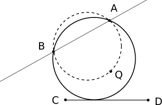
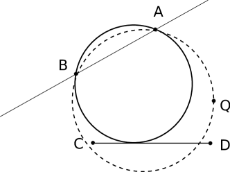
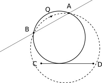
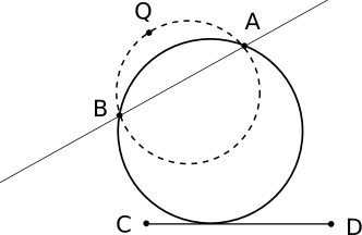
Figure 3: Reducing $\textsf{Incircle}(A,B,CD,Q)$ to $\textsf{Incircle}(A,B,Q,CD)$. Top/Bottom row: $Q$ lies to the left/right of the oriented line $\ell_{AB}$. Left/Right column: $Q$ lies inside/outside $V(A,B,CD)$. The dotted circle is the Voronoi circle of $A$, $B$ and $Q$.

Let $Q$ be the query point, and $K$ be the center of $V(A,B,CD)$. As we will see in the next subsection, the $x$-coordinate of $K$ is a root of a quadratic equation $P(x)=p_{2}x^{2}+p_{1}x+p_{0}$, where the algebraic degrees of $p_{2}$, $p_{1}$ and $p_{0}$ are 1, 2 and 3, respectively. Moreover, in this case $y_{K}=\frac{\alpha_{1}}{\beta}x_{K}+\frac{\alpha_{0}}{\beta}$, where the algebraic degrees of $\alpha_{1}$, $\alpha_{0}$ and $\beta$ are 1, 2 and 1, respectively (i.e., $\delta_{\alpha}=\delta_{x}=1$). By Subsection 5.1 we can evaluate $\textsf{Incircle}(A,B,CD,Q)$ using algebraic expressions of maximum degree $2\cdot{}1+1+4=7$. Below, we are going to show how to lower this maximum algebraic degree to 6.

Clearly, for the Voronoi circle $V(A,B,CD)$ to be defined, both $A$ and $B$ must be on the same side with respect to $\ell_{CD}$. Consider now $Q$: if $Q$ does not lie on the side of $\ell_{CD}$ that $A$ and $B$ lie, we have $\textsf{Incircle}(A,B,CD,Q)>0$. Testing the sideness of $I$, $I\in\{A,B,Q\}$, against $\ell_{CD}$ simply means testing the sign of $y_{I}-y_{C}$, which is a quantity of algebraic degree 1.

Suppose now that $Q$ lies on the same side of $\ell_{CD}$ as $A$ and $B$, and assume, without loss of generality, that $\textsf{Orientation}(A,C,D)>0$ (the argument in the case $\textsf{Orientation}(A,C,D)<0$, or when one of $A$ and $B$ lies on $\ell_{CD}$, is analogous). Consider the result $\sigma$ of the orientation predicate $\textsf{Orientation}(A,B,Q)$. In the special case $\sigma=0$ (i.e., $Q$ lies on the line $\ell_{AB}$), we observe that $Q$ lies inside the Voronoi circle $V(A,B,CD)$ if and only if $Q$ lies on $\ell_{AB}$ and between $A$ and $B$. This can be determined by evaluating the signs of differences $x_{Q}-x_{A}$ and $x_{Q}-x_{B}$, which are both quantities of algebraic degree 1.

If $\sigma\neq{}0$, we are going to reduce $\textsf{Incircle}(A,B,CD,Q)$ to $\textsf{Incircle}(A,B,Q,CD)$ (see also Fig. 3). Suppose first that $\sigma>0$, i.e., $Q$ lies to the left of the oriented line $\ell_{AB}$. Since $A$, $B$ and $CD$ appear on $V(A,B,CD)$ in that order when we traverse it in the counterclockwise sense, we conclude that $Q$ lies inside $V(A,B,CD)$ (resp., lies on $V(A,B,CD)$) if and only if the circle defined by $A$, $B$ and $Q$, does not intersect with (resp., touches) the line $\ell_{CD}$. To see this, simply “push” the Voronoi circle towards $Q$, while keeping its center on the bisector of $A$ and $B$. Hence, $\textsf{Incircle}(A,B,CD,Q)=-\textsf{Incircle}(A,B,Q,CD)$. In a similar manner, if $\sigma<0$, i.e., $Q$ lies to the right of the oriented line $\ell_{AB}$, $Q$ lies inside $V(A,B,CD)$ (resp., lies on $V(A,B,CD)$) if and only if the circle defined by $A$, $B$ and $Q$ intersects the line $\ell_{CD}$. Hence, $\textsf{Incircle}(A,B,CD,Q)=\textsf{Incircle}(B,A,Q,CD)$.

Summarizing our analysis above, we first need to determine on which side of $\ell_{CD}$ $Q$ lies: this a degree 1 predicate. If needed, the next step is to compute $\textsf{Orientation}(A,B,Q)$, which is a degree 2 predicate. If $\textsf{Orientation}(A,B,Q)=0$ we need two additional tests of degree 1 to answer $\textsf{Incircle}(A,B,CD,Q)$; otherwise, we observe that

$$\textsf{Incircle}(A,B,CD,Q)=\begin{cases}-\textsf{Incircle}(A,B,Q,CD),&\text{if\ }\textsf{Orientation}(A,B,Q)>0\\ {\color[rgb]{1,1,1}-}\textsf{Incircle}(B,A,Q,CD),&\text{if\ }\textsf{Orientation}(A,B,Q)<0\end{cases}$$

As per Section 3.2, $\textsf{Incircle}(A,B,Q,CD)$ or $\textsf{Incircle}(B,A,Q,CD)$ can be answered using quantities of algebraic degree at most 6.

6.2 The query object is a segment

For this case we are going to follow the generic analysis presented in Section 5.2. Let $QS$ be the query segment, and let $K$ be the center of $V(A,B,CD)$. $K$ is an intersection point of the bisector of $A$ and $B$ and the parabola with focal point $A$ and directrix the supporting line $\ell_{CD}$ of $CD$. Solving the corresponding system of equations we deduce that, in the general case where $A$ and $B$ are not equidistant from $\ell_{CD}$ (i.e., if $y_{A}\neq{}y_{B}$), the $x$-coordinate of the Voronoi center $x_{K}$, is a root of the quadratic polynomial $P(x)=p_{2}x^{2}+p_{1}x+p_{0}$, where $p_{2}=y_{B}-y_{A}\neq{}0$, $p_{1}=(y_{B}-y_{C})(x_{A}-x_{B})-2x_{B}p_{2}$, $p_{0}=p_{2}x_{B}^{2}+(y_{C}-y_{B})[(x_{B}^{2}-x_{A}^{2})+(y_{A}-y_{C})p_{2}]$, while the $y$-coordinate of the Voronoi center $y_{K}$, is a root of the quadratic polynomial $T(y)=t_{2}y^{2}+t_{1}y+t_{0}$, where $t_{2}=4(y_{B}-y_{A})^{2}$, $t_{1}=4(2y_{C}-y_{A}-y_{B})(x_{B}-x_{A})^{2}+4(y_{B}-y_{A})(y_{A}^{2}-y_{B}^{2})$, $t_{0}=(x_{A}-x_{B})^{2}(2y_{A}^{2}+2y_{B}^{2}-4y_{C}^{2}+(x_{A}-x_{B})^{2})+(y_{A}^{2}-y_{B}^{2})^{2}$. Moreover, $y_{K}$ and $x_{K}$ are linearly dependent: $y_{K}=\frac{\alpha_{1}}{\beta}x_{K}+\frac{\alpha_{0}}{\beta}$, where $\alpha_{1}=2(x_{A}-x_{B})$, $\alpha_{0}=x_{B}^{2}+y_{B}^{2}-x_{A}^{2}-y_{A}^{2}$ and $\beta=2(y_{B}-y_{A})$. The roots $x_{1}\leq{}x_{2}$ of the polynomial $P(x)$ (resp. $y_{1}\leq{}y_{2}$ of $T(y)$) correspond to the centers of the two possible Voronoi circles $V(A,B,CD)$ and $V(B,A,CD)$. The roots of $P(x)$ or of $T(y)$) of interest are shown in the following two tables.

Relative positions of $A$, $B$ and $CD$	Root of $P(x)$ of interest
$y_{C}<y_{A}<y_{B}$	$x_{1}$
$y_{C}<y_{B}<y_{A}$	$x_{2}$
$y_{B}<y_{A}<y_{C}$	$x_{2}$
$y_{A}<y_{B}<y_{C}$	$x_{1}$

Relative positions of $A$, $B$	Root of $T(y)$ of interest
$x_{A}<x_{B}$	$y_{2}$
$x_{A}>x_{B}$	$y_{1}$

The degrees of $p_{2}$, $p_{1}$, $p_{0}$, $t_{2}$, $t_{1}$ and $t_{0}$ are 1, 2, 3, 2, 3 and 4, respectively. Furthermore, the degrees of $\alpha_{1}$, $\alpha_{0}$ and $\beta$ are 1, 2 and 1, respectively. Applying the analysis in Subsection 5.2 (where $\delta_{\alpha}=\delta_{x}=1$, $\delta_{y}=2$), we deduce that we can answer the Incircle predicate using expressions of algebraic maximum algebraic degree $\max\{2\cdot{}1+1+2,2+2\}=5$.

For the special case $y_{A}=y_{B}$, we easily get $x_{K}=\frac{1}{2}(x_{A}+x_{B})$ and $y_{K}=\frac{U_{2}}{U_{1}}$, where $U_{2}=(x_{B}-x_{A})^{2}+4(y_{A}^{2}-y_{C}^{2})$, $U_{1}=8(y_{A}-y_{C})$. In this case, if $QS$ is $x$-axis parallel, we need to determine the sign of the quantity $d(K,\ell_{QS})-d(K,CD)=|y_{K}-y_{Q}|-|y_{K}-y_{C}|$, or, equivalently, the sign of the quantity $|U_{2}-U_{1}y_{Q}|-|U_{2}-U_{1}y_{C}|$, which is of algebraic degree 2. If $QS$ is $y$-axis parallel, we need to evaluate the sign of the quantity $d(K,\ell_{QS})-d(K,CD)=|x_{K}-x_{Q}|-|y_{K}-y_{C}|$, or, equivalently, the sign of the quantity $|U_{1}(x_{A}+x_{B}-2x_{Q})|-2|U_{2}-U_{1}y_{Q}|$, which is also of algebraic degree 2. Given, that the algebraic degree for the $PPSP$ case is 6 (see previous subsection), we conclude that we can answer the Incircle predicate in the $PPSS$ case by computing the signs of expressions of algebraic degree at most 6.

7 The $PSS$ case

7.1 The query object is a point

In this section we consider the case where the Voronoi circle is defined by two segments, a point and the query object is a point. Let $A$, $CD$ and $FG$ be the point and the two segments defining the Voronoi circle and let $Q$ be the query point. Since each of $CD$, $FG$ may be $x$-axis or $y$-axis parallel we have four cases to consider: (1) $CD$ and $FG$ are $x$-axis parallel, (2) $CD$ and $FG$ are $y$-axis parallel, (3) $CD$ is $x$-axis parallel and $FG$ is $y$-axis parallel, and (4) $CD$ is $y$-axis parallel and $FG$ is $x$-axis parallel. However, Cases (2) and (4) reduce to Cases (1) and (4), respectively, by simply performing a reflection transformation through the line $y=x$ (see Section 2.2). More precisely, in both cases we have $\textsf{Incircle}(A,CD,FG,Q)=\textsf{Incircle}(\mathcal{R}(A),\mathcal{R}(FG),\mathcal{R}(CD),\mathcal{R}(Q))$. Thus, for Case (2), $\mathcal{R}(CD)$ and $\mathcal{R}(FG)$ are $x$-axis parallel, while, for Case (4), $\mathcal{R}(CD)$ is $x$-axis parallel and $\mathcal{R}(FG)$ is $y$-axis parallel. Therefore it suffices to consider Cases (1) and (3). In what follows, we follow the generic procedure described in Subsection 5.1, and refer to the notation introduced there.

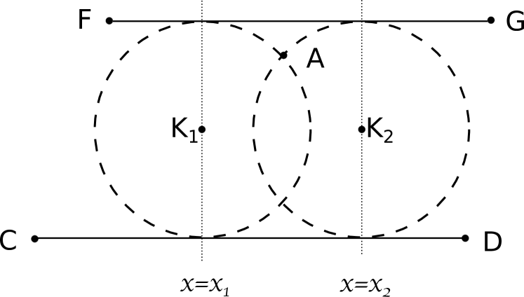
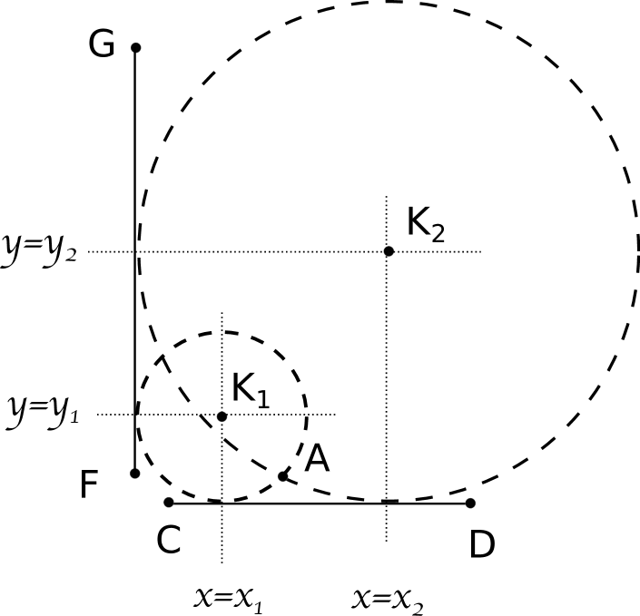
Figure 4: Voronoi circle defined by the point $A$ and the line segments $CD$ and $FG$. Left: $CD$, $FG$ are $x$-axis parallel. Right: $CD$ is $x$-axis parallel and $FG$ is $y$-axis parallel.

7.1.1 $CD$ and $FG$ are $x$-axis parallel

We first notice that if $Q$ does not lie inside the band $B_{x}$ delimited by the $\ell_{CD}$ and $\ell_{FG}$, it cannot be inside the Voronoi circle $V(A,CD,FG)$. This can be easily checked by evaluating the signs of $y_{Q}-y_{C}$ and $y_{Q}-y_{F}$, which are quantities of algebraic degree 1. Suppose now that $Q$ is inside $B_{x}$ and notice that $A$ has to lie in $B_{x}$ in order for the Voronoi circle $V(A,CD,FG)$ to exist.

Let $K$ be the center of $V(A,CD,FG)$. The $y$-coordinate of $K$ is, trivially, $y_{K}=\frac{1}{2}(y_{C}+y_{F})$, whereas the radius $\rho$ of the Voronoi circle is equal to $\rho=\frac{1}{2}|y_{C}-y_{F}|$. Given that $A$ is a point on $V(A,CD,FG)$, we have that $d^{2}(K,A)=\rho^{2}$. Using the expressions for $y_{K}$ and $\rho$, we deduce that $x_{K}$ is a root of the polynomial $P(x)=x^{2}+p_{1}x+p_{0}$, where $p_{1}=2x_{A}$ and $p_{0}=x_{A}^{2}+(y_{A}-y_{C})(y_{A}-y_{F})$. If $x_{1}\leq{}x_{2}$ are the two roots of $P(x)$, the root that corresponds to $x_{K}$ is given in the table below (see also Fig. 4(left)).

Relative positions of $A$ and $CD$	Root of $P(x)$ of interest
$y_{A}>y_{C}$	$x_{2}$
$y_{A}<y_{C}$	$x_{1}$

Moreover, in this case we have $\alpha_{1}=0$, $\alpha_{0}=y_{C}+y_{F}$ and $\beta=2$. Therefore, the algebraic degrees involved in the evaluation of the Incircle predicate are $\delta_{\alpha}=\delta_{x}=0$. As per Subsection 5.1, the $\textsf{Incircle}(A,CD,FG,Q)$ predicate can be evaluated using algebraic expressions of maximum degree $2\cdot{}0+0+4=4$.

7.1.2 $CD$ is $x$-axis parallel and $FG$ is $y$-axis parallel

The lines $\ell_{CD}$ and $\ell_{FG}$ subdivide the plane into four quadrants $R_{1}$, $R_{2}$, $R_{3}$ and $R_{4}$. The bisector of $R_{1}$ and $R_{3}$ is the line $\ell_{1,3}$ with equation $y=x+y_{C}-x_{F}$, whereas the bisector of $R_{2}$ and $R_{4}$ is the line $\ell_{2,4}$ with equation $y=-x+y_{C}+x_{F}$.

The center $K$ of the Voronoi circle $V(A,CD,FG)$ lies on both the bisector of $\ell_{CD}$ and $\ell_{FG}$, as well as on the parabola that is at equal distance from $A$ and $\ell_{CD}$; the equation of the latter is:

$$(x-x_{A})^{2}-(y_{A}-y_{C})(2y-y_{A}-y_{C})=0.$$ (3)

Assuming that $A$ lies in $R_{1}\cup{}R_{3}$, the bisector of $\ell_{CD}$ and $\ell_{FG}$ is $\ell_{1,3}$. Substituting $y$ in terms of $x$, using the equation of $\ell_{1,3}$, we deduce that the $x$-coordinate $x_{K}$ of $K$ is a root of the quadratic polynomial $P(x)=x^{2}+p_{1}x+p_{0}$, where $p_{1}=2(y_{C}-y_{A}-x_{A})$, and $p_{0}=(y_{C}-y_{A})^{2}+x_{A}^{2}-2x_{F}(y_{C}-y_{A})$. Similarly, if $A$ lies in $R_{2}\cup{}R_{4}$, $x_{K}$ is a root of the quadratic polynomial $P(x)=x^{2}+p_{1}x+p_{0}$, where $p_{1}=2(y_{A}-y_{C}-x_{A})$, $p_{0}=(y_{C}-y_{A})^{2}+x_{A}^{2}+2x_{F}(y_{C}-y_{A})$. If $x_{1}\leq{}x_{2}$ are the two roots of $P(x)$, the root that corresponds to $x_{K}$ is the same as in the case where $FG$ is $x$-axis parallel. Moreover, in this case we have $\alpha_{1}=1$, $\alpha_{0}=y_{C}-x_{F}$, $\beta=1$, if $A\in{}R_{1}\cup{}R_{3}$, and $\alpha_{1}=-1$, $\alpha_{0}=y_{C}+x_{F}$, $\beta=1$, if $A\in{}R_{2}\cup{}R_{4}$. In both cases, the algebraic degrees involved in the evaluation of the Incircle predicate are $\delta_{\alpha}=\delta_{x}=0$. Again, as per Subsection 5.1, the $\textsf{Incircle}(A,CD,FG,Q)$ predicate can be evaluated using algebraic expressions of maximum degree $2\cdot{}0+0+4=4$.

7.2 The query object is a segment

Let $QS$ be the query segment, while the Voronoi circle is defined by the point $A$ and the segments $CD$ and $FG$. Let $K=(x_{K},y_{K})$ be the center of the Voronoi circle. As in the previous subsection, it suffices to consider the cases where, either both $CD$ and $FG$ are $x$-axis parallel, or $CD$ is $x$-axis parallel and $FG$ is $y$-axis parallel. Recall that, in both cases, we have shown that $x_{K}$ is always a root of a quadratic polynomial $P(x)=x^{2}+p_{1}x+p_{0}$, where the algebraic degrees of $p_{1}$ and $p_{0}$ are 1 and 2, respectively.

7.2.1 $CD$ and $FG$ are $x$-axis parallel

If $QS$ is also $x$-axis parallel we first need to determine if $QS$ lies inside the band $B_{x}$ delimited by $\ell_{CD}$ and $\ell_{FG}$. This is easily done by checking if $Q$ lies inside $B_{x}$, which in turn means checking the signs of $y_{Q}-y_{C}$ and $y_{Q}-y_{F}$, as described in the previous subsection. Clearly, if $Q$ is not inside the band $B_{x}$, then $\textsf{Incircle}(A,CD,FG,QS)>0$. Assume now that $QS$ lies inside $B_{x}$. The first step is to evaluate the $\textsf{Incircle}(A,CD,FG,Q)$ and, if necessary, $\textsf{Incircle}(A,CD,FG,S)$. If $\textsf{Incircle}(A,CD,FG,Q)<0$ or $\textsf{Incircle}(A,CD,FG,S)<0$, then we immediately know that $\textsf{Incircle}(A,CD,FG,QS)<0$. Otherwise, we simply need to determine on which side of the line $x=x_{K}$ $Q$ and $S$ lie: $QS$ intersects the Voronoi circle $V(A,CD,FG)$ if and only if $Q$ and $S$ lie on different sides of $x=x_{K}$. Determining the side of $x=x_{K}$ on which the point $I$, $I\in\{Q,S\}$, lies is equivalent to computing the sign of the difference $x_{K}-x_{I}$. This, in turn, reduces to computing the signs of the expressions $P(x_{I})$ and $P^{\prime}(x_{I})$, which are expressions of algebraic degree 2 and 1, respectively.

In the case where $QS$ is $y$-axis parallel, we proceed according to the generic approach presented in Subsection 5.2. In this case $y_{K}=\frac{1}{2}(y_{C}+y_{F})$, i.e., $\alpha_{1}=0$, $\alpha_{0}=y_{C}+y_{F}$ and $\beta=2$. Moreover, $T(y)$ is a linear polynomial $T(y)=2y-(y_{C}+y_{F})$, thus the algebraic degrees of $T(y_{I})$ and $T^{\prime}(y_{I})$, $I\in\{Q,S\}$, are $\delta_{y}+1=1$ and $\delta_{y}=0$, respectively. By applying the analysis of Subsection 5.2, with $\delta_{x}=\delta_{\alpha}=\delta_{y}=0$, we conclude that we can answer the Incircle predicate by evaluating the signs of expressions of algebraic degree at most $\max\{2\cdot{}0+0+4,0+1\}=4$.

7.2.2 $CD$ is $x$-axis parallel and $FG$ is $y$-axis parallel

For the purposes of resolving this case, we are going to follow the analysis of Subsection 5.2. In the previous subsection we argued that in this case the center $K=(x_{K},y_{K})$ of the Voronoi circle $V(A,CD,FG)$ lies on the intersection of the parabola with equation (3) and either the line $y=x+y_{C}-x_{F}$ (if $A\in{}R_{1}\cup{}R_{3}$) or the line $y=-x+y_{C}+x_{F}$ (if $A\in{}R_{2}\cup{}R_{4}$). Solving in terms of $y$ we deduce that $y_{K}$ is a root of the quadratic polynomial $T(y)=y^{2}+t_{1}y+t_{0}$, where $t_{1}=-2(y_{A}+x_{A}+x_{F}-2y_{C})$, $t_{0}=(x_{A}+x_{F})^{2}+y_{A}^{2}-2y_{C}(x_{A}+x_{F})$, if $A\in{}R_{1}\cup{}R_{3}$, whereas $t_{1}=2(x_{A}-y_{A}-x_{F})$, $t_{0}=(x_{A}-x_{F})^{2}+y_{A}^{2}-2x_{A}y_{C}+2y_{C}x_{F}$, if $A\in{}R_{2}\cup{}R_{4}$. Notice that in both cases the algebraic degrees of $t_{1}$ and $t_{0}$ are 1 and 2, respectively. Furthermore, if $y_{1}\leq{}y_{2}$ are the two roots of $T(y)$, the root of $T(y)$ of interest is given in the following table (see also Fig. 4(right)).

Relative positions of $A$ and $FG$	Root of $T(y)$ of interest
$x_{A}>x_{F}$	$y_{2}$
$x_{A}<x_{F}$	$y_{1}$

Finally, as already described in the previous subsection, in this case we have $\alpha_{1}=1$, $\alpha_{0}=y_{C}-x_{F}$, $\beta=1$, if $A\in{}R_{1}\cup{}R_{3}$, and $\alpha_{1}=-1$, $\alpha_{0}=y_{C}+x_{F}$, $\beta=1$, if $A\in{}R_{2}\cup{}R_{4}$. We are now ready to apply the analysis of Subsection 5.2, with $\delta_{\alpha}=\delta_{x}=\delta_{y}=0$. We thus conclude that the predicate $\textsf{Incircle}(A,CD,FG,QS)$ can be evaluated using algebraic quantities of degree at most $\max\{2\cdot{}0+0+4,0+2\}=4$.

8 Conclusion and future work

In this paper we have studied the Incircle predicate involved in the computation of the Euclidean Voronoi diagram for axes-aligned line segments. We have described in detail, and in a self-contained manner, how to evaluate this predicate. We have shown that we can always resolve it using polynomial expressions in the input quantities that are of maximum algebraic degree 6.

Our analysis is thus far theoretical. We would like to implement the approach presented in this paper and compare it against the generic implementation in CGAL [13]. Finally, we would like to study the rest of the predicates involved in the computation of the Voronoi diagram, as well as consider the ortho-45^∘ case, i.e., the case where the segments are allowed to lie on lines parallel to the lines $y=x$ and $y=-x$.

References

- [1] J.-D. Boissonnat, O. Devillers, R. Schott, M. Teillaud, and M. Yvinec. Applications of random sampling to on-line algorithms in computational geometry. Discrete Comput. Geom., 8:51–71, 1992.
- [2] J.-D. Boissonnat and F.P. Preparata. Robust plane sweep for intersecting segments. SIAM J. Comput., 29(5):1401–1421, 2000.
- [3] J.-D. Boissonnat and M. Yvinec. Algorithmic Geometry. Cambridge University Press, UK, 1998. Translated by Hervé Brönnimann.
- [4] C. Burnikel. Exact Computation of Voronoi Diagrams and Line Segment Intersections. Ph.D thesis, Universität des Saarlandes, March 1996.
- [5] O. Devillers, A. Fronville, B. Mourrain, and M. Teillaud. Algebraic methods and arithmetic filtering for exact predicates on circle arcs. Comp. Geom: Theory & Appl., Spec. Issue, 22:119–142, 2002.
- [6] R. L. Drysdale, III and D. T. Lee. Generalized Voronoi diagrams in the plane. In Proc. 16th Allerton Conf. Commun. Control Comput., pages 833–842, 1978.
- [7] Ioannis Z. Emiris and Menelaos I. Karavelas. The predicates of the Apollonius diagram: algorithmic analysis and implementation. Computational Geometry: Theory and Applications, 33(1-2):18–57, January 2006. Special Issue on Robust Geometric Algorithms and their Implementations.
- [8] S. J. Fortune. A sweepline algorithm for Voronoi diagrams. Algorithmica, 2:153–174, 1987.
- [9] Chris Gold. The Dual is the Context: Spatial Structures for GIS. In Proceedings of the 7th International Symposium on Voronoi Diagrams in Science and Engineering (VD2010), pages 3–10, Québec City, Québec, Canada, June 28–30, 2010.
- [10] Puneet Gupta and Evanthia Papadopoulou. Yield analysis and optimization. In C.J. Alpert, D.P. Mehta, and S.S. Sapatnekar, editors, The Handbook of Algorithms for VLSI Physical Design Automation, chapter 7.3. Taylor & Francis CRC Press, November 2008.
- [11] M. Held. VRONI: An engineering approach to the reliable and efficient computation of Voronoi diagrams of points and line segments. Comput. Geom. Theory Appl., 18:95–123, 2001.
- [12] T. Imai. A topology oriented algorithm for the Voronoi diagram of polygons. In Proc. 8th Canad. Conf. Comput. Geom., pages 107–112. Carleton University Press, Ottawa, Canada, 1996.
- [13] Menelaos Karavelas. 2D segment Delaunay graphs. In CGAL User and Reference Manual. CGAL Editorial Board, 3.7 edition, 2010.
- [14] Menelaos I. Karavelas. A robust and efficient implementation for the segment Voronoi diagram. In Proceedings of the International Symposium on Voronoi Diagrams in Science and Engineering (VD2004), pages 51–62, Hongo, Tokyo, Japan, September 13–15, 2004.
- [15] Menelaos I. Karavelas and Ioannis Z. Emiris. Root comparison techniques applied to the planar additively weighted Voronoi diagram. In Proc. 14th ACM-SIAM Symp. on Discrete Algorithms (SODA), pages 320–329, January 2003.
- [16] D. G. Kirkpatrick. Efficient computation of continuous skeletons. In Proc. 20th Annu. IEEE Sympos. Found. Comput. Sci., pages 18–27, 1979.
- [17] R. Klein, K. Mehlhorn, and S. Meiser. Randomized incremental construction of abstract Voronoi diagrams. Comput. Geom.: Theory & Appl., 3(3):157–184, 1993.
- [18] D. T. Lee. Medial axis transformation of a planar shape. IEEE Trans. Pattern Anal. Mach. Intell., PAMI-4(4):363–369, 1982.
- [19] G. Liotta, F.P. Preparata, and R. Tamassia. Robust proximity queries: An illustration of degree-driven algorithm design. SIAM J. Comput., 28(3):864–889, 1999.
- [20] David L. Millman and Jack Snoeyink. Computing planar Voronoi diagrams in double precision: a further example of degree-driven algorithm design. In Proceedings of the 26th Annual Symposium on Computational Geometry (SoCG’10), pages 386–392, Snowbird, Utah, USA, 2010.
- [21] Evanthia Papadopoulou. Critical area computation for missing material defects in VLSI circuits. IEEE Trans. on CAD of Integrated Circuits and Systems, 20(5):583–597, 2001.
- [22] M. Seel. The AVD LEP user manual.
- [23] K. Sugihara, M. Iri, H. Inagaki, and T. Imai. Topology-oriented implementation - an approach to robust geometric algorithms. Algorithmica, 27(1):5–20, 2000.
- [24] C. K. Yap. An algorithm for the Voronoi diagram of a set of simple curve segments. Discrete Comput. Geom., 2:365–393, 1987.
- [25] C. K. Yap and T. Dubé. The exact computation paradigm. In D.-Z. Du and F. K. Hwang, editors, Computing in Euclidean Geometry, volume 4 of Lecture Notes Series on Computing, pages 452–492. World Scientific, Singapore, 2nd edition, 1995.