Abstract

We discuss the choice of input parameters for the renormalization of the chargino and neutralino sector in the minimal supersymmetric standard model (MSSM) in the on–shell scheme. We show that one should chose the masses of a bino–like, a wino–like and a higgsino–like state as inputs in order to avoid large corrections to the masses of the other eigenstates in this sector. We also show that schemes where the higgsino–like input state is a neutralino are more stable than those where the mass of the higgsino–like chargino is used as input. The most stable scheme uses the masses of the wino–like chargino as well as the masses of the bino– and higgsino–like neutralinos as inputs.

1 Introduction

Among possible solutions of the hierarchy problem [1, 2, 3, 4], supersymmetric extensions of the Standard Model (SM) of particle physics [5, 6] have the advantage that effects of the hypothetical new “superparticles” required in these constructions can be computed perturbatively. This distinguishes them e.g. from scenarios where electroweak symmetry breaking is accomplished by some new strong dynamics. At the same time, future measurements at the LHC [7] and a possible $e^{+}e^{-}$ linear collider [8] can easily have statistical uncertainties at or below the percent level, making correspondingly accurate theoretical calculations highly desirable. This will require the calculation of electroweak corrections at least at the one–loop level. Independent motivation for such calculations comes from the possibility that neutralinos form the dark matter in the universe, since the determination of the overall dark matter density of the universe has now been determined with an error of a few percent [9].

In all these cases the renormalization of the chargino and neutralino sector plays a central role. In most SUSY breaking scenarios the lighter charginos and neutralinos are among the lighter superparticles, i.e. among the first ones to be discovered by future $e^{+}e^{-}$ supercolliders. At the LHC the most important search channels start from the production of squarks and gluinos, which subsequently decay into charginos and/or neutralinos.

The renormalization scheme of choice is on–shell renormalization, for (at least) two reasons. First, there is a fairly direct relation between the physical chargino and neutralino masses and the parameters that need to be renormalized; this relation becomes trivial in the limit where the spontaneous breaking of the electroweak gauge symmetry can be neglected. Moreover, masses will probably be among the first quantities that are measured accurately.

The on–shell renormalization of the neutralino and chargino sectors in the minimal supersymmetric standard model (MSSM) with conserved $R-$parity has been discussed in [10, 11, 12]. In full generality, the chargino and neutralino mass matrices depend on six independent parameters that need to be renormalized. However, two of these (the masses of the $W$ and $Z$ bosons) already appear in the SM; they are renormalized through the same conditions as in the SM (albeit with additional contributions to the relevant two–point functions with superparticles in the loop). A third parameter, the ratio of vacuum expectation values (VEVs) $\tan\beta$, is usually renormalized in the MSSM Higgs sector. This leaves only three independent parameters whose renormalization has to be fixed through on–shell conditions for charginos and neutralinos. This means that only three of the six chargino and neutralino masses can be used as independent input parameters; their values are exact to all orders in the on–shell scheme. The other three masses can then be predicted, but the numerical values of these predictions are subject to loop corrections.

Previously different calculations used different sets of input masses, corresponding to different variants of the on–shell scheme. For example, in ref. [10], both chargino masses and the lightest neutralino mass are used as inputs. In [13] the decay of the next to lightest neutralino to the lightest neutralino was studied at one loop level using the on–shell renormalization scheme. The input masses were conveniently assumed to be the masses of the two lightest neutralinos and the heaviest chargino.

Since the lighter neutralino states are more accessible at colliders, using their masses as inputs seems favorable from the experimental point of view. However, reliable perturbative predictions can be made only if the perturbative expansion is stable, i.e. if loop corrections are not very large. From this point of view using the masses of both charginos and the lightest neutralino as input can be problematic: the corrections to the masses of some of the other three neutralinos can become large if the lightest neutralino is an almost pure higgsino or wino [14, 15]. The reason is that all three input masses then only depend very weakly on the $U(1)_{Y}$ gaugino (bino) mass parameter. A large (finite part of the) counterterm may therefore be needed in order to correct small loop corrections to the input masses, so that these masses remain unchanged, as required in on–shell renormalization; the large counterterm will then lead to large changes of other neutralino masses. By a very similar argument, in this situation small experimental errors on the input masses can lead to very large errors on the bino mass parameter even when quantum corrections are neglected. An analogous instability can arise when using the masses of the two lightest neutralinos and the heavier chargino as inputs. Note also that both these schemes require the mass of the heavier chargino as input, which is one of the heaviest states in this sector; this considerably weakens the argument in favor of using only the masses of the lighter neutralino states as inputs.

If the mass of the higgsino–like chargino is used as input an additional perturbative instability occurs if the $SU(2)$ gaugino (wino) and higgsino mass parameters are of similar magnitude. It has been noticed in [10, 14, 15] that using both chargino masses as input leads to undefined renormalized masses for exact equality of the absolute values of the wino and higgsino mass parameters; not surprisingly, corrections remain very large, albeit finite, if the difference between these two parameters is nonzero but small. We find that this instability also occurs in schemes where the mass of the higgsino–like chargino and two neutralino masses are used as inputs.

In this paper we address these two stability issues by explicitly calculating chargino and neutralino masses at one–loop level using the on–shell renormalization scheme. We compare seven different choices for the three input masses, combining two, one or zero chargino masses with either the mass(es) of the lightest neutralino state(s) or with the masses of neutralino states of given character (bino–, wino– or higgsino–like). We demonstrate explicitly that the choice of any three input masses, which include a higgsino–like, a wino–like and a bino–like mass eigenstate, avoids the first instability, independent of whether chargino or neutralino masses are used. Requiring in addition perturbative stability also for similar magnitudes of the wino and higgsino mass parameters singles out schemes where the masses of the (most) bino– and higgsino–like neutralinos are used as inputs. Schemes using three neutralino masses as inputs show an additional, but much weaker, instability for approximately equal $SU(2)$ and $U(1)_{Y}$ gaugino masses; this second instability is absent if the mass of the wino–like chargino, rather than that of the wino–like neutralino, is used as input together with the two neutralino masses listed above.

In this paper we assume all relevant mass parameters to be real. Experimental constraints on CP violation, mainly from EDM measurements, require their phases to be small, unless superpartners of first (and second) generation fermions are very heavy [16, 17].

This article is organized as follows. In Section 2 we discuss briefly seven different variants of the on–shell scheme, in the context of the MSSM with exact $R-$parity. Section 3 discusses the practical implementation of our schemes. In Section 4 we compare the above seven schemes, defined by different sets of input masses. Explicit expressions for the counterterms in schemes where two or three neutralino masses are used as inputs are given in Appendices A and B, respectively, while Appendix C shows how to distinguish the wino– and higgsino–like chargino state using $Z\tilde{\chi}^{+}\tilde{\chi}^{-}$ couplings.

2 Formalism

In this section we discuss the on–shell renormalization of the chargino and neutralino sector of the MSSM with exact $R-$parity [10, 15]. To this end we first review tree–level results for chargino and neutralino masses and mixings. We then describe general features of the on–shell renormalization scheme as applied to this sector, before introducing three variants of this scheme, each of which has two or three subvariants.

2.1 Tree–Level Results

The tree level mass terms for the charginos, in the gauge eigenbasis, can be written as [5]

$$-\mathcal{L}^{\rm c}_{\rm mass}=\psi^{-T}M^{c}\psi^{+}+h.c.$$ (1)

where

$$\psi^{+}=(\widetilde{W}^{+},~{}~{}\tilde{h}^{+}_{2})^{T},~{}~{}\psi^{-}=(\widetilde{W}^{-},~{}~{}\tilde{h}^{-}_{1})^{T}$$ (2)

are column vectors whose components are Weyl spinors. The mass matrix $M^{\rm c}$ is given by

$$M^{\rm c}=\left(\begin{array}[]{cc}M_{2}&\sqrt{2}M_{W}\sin\beta\\ \sqrt{2}M_{W}\cos\beta&\mu\\ \end{array}\right).$$ (3)

Here $M_{2}$ is the SUSY breaking $SU(2)$ gaugino (wino) mass, $\mu$ is the supersymmetric higgsino mass, $M_{W}$ is the mass of the $W$ boson, and $\tan\beta$ is the ratio of VEVs of the two neutral Higgs fields of the MSSM. $M^{\rm c}$ may be diagonalized using unitary matrices $U$ and $V$ to obtain the diagonal mass matrix,

$$M^{\rm c}_{D}=U^{*}M^{\rm c}V^{-1}=\left(\begin{array}[]{cc}m_{\tilde{\chi}_{1}^{+}}&0\\ 0&m_{\tilde{\chi}_{2}^{+}}\\ \end{array}\right).$$ (4)

Without loss of generality, we order the eigenstates such that $0<m_{\tilde{\chi}_{1}^{+}}\leq m_{\tilde{\chi}_{2}^{+}}$. Note that scenarios with $m_{\tilde{\chi}_{1}^{+}}\>\raisebox{-2.15277pt}{$\stackrel{{\scriptstyle\textstyle<}}{{\sim}}$}\>100$ GeV are excluded by chargino searches at LEP [18]. The left– and right–handed components of the corresponding Dirac mass eigenstates, the charginos $\tilde{\chi}^{+}_{i}$ with $i=1$ or $2$, are

$$P_{L}\tilde{\chi}^{+}_{i}=V_{ij}\psi^{+}_{j},~{}~{}P_{R}\tilde{\chi}^{+}_{i}=U^{*}_{ij}\overline{\psi^{-}_{j}}\,,$$ (5)

where $P_{L}$ and $P_{R}$ are chiral projectors, $\overline{\psi^{-}_{j}}$ is the hermitean conjugate of the Weyl fermion $\psi^{-}_{j}$, and summation over $j$ is understood in Eqs.(5).

In the gauge eigenbasis, the tree level neutralino mass terms are given by [5]

$$-\mathcal{L}^{\rm n}_{\rm mass}=\frac{1}{2}\psi^{0T}M^{n}\psi^{0}+h.c.,$$ (6)

where

$$\psi^{0}=\left(\begin{array}[]{cccc}\tilde{B^{0}},&\widetilde{W}^{3},&\tilde{h}_{1}^{0},&\tilde{h}_{2}^{0}\end{array}\right)^{T},$$ (7)

is again a column vector whose components are Weyl fermions, and the neutralino mass matrix $M^{\rm n}$ is given by

$$M^{\rm n}=\left(\begin{array}[]{cccc}M_{1}&0&-M_{Z}s_{W}c_{\beta}&M_{Z}s_{W}s_{\beta}\\ 0&M_{2}&M_{Z}c_{W}c_{\beta}&-M_{Z}c_{W}s_{\beta}\\ -M_{Z}s_{W}c_{\beta}&M_{Z}c_{W}c_{\beta}&0&-\mu\\ M_{Z}s_{W}s_{\beta}&-M_{Z}c_{W}s_{\beta}&-\mu&0\end{array}\right)\,.$$ (8)

Here $s_{W},s_{\beta},c_{W}$ and $c_{\beta}$ stand for $\sin\theta_{W},\sin\beta,\cos\theta_{W}$ and $\cos\beta$, respectively, where $\theta_{W}$ is the weak mixing angle. $M_{Z}$ is the mass of the $Z$ boson, and $M_{1}$ is the SUSY breaking $U(1)_{Y}$ gaugino (bino) mass. Finally, $M_{2}$ and $\mu$ already appeared in the chargino mass matrix (3).

$M^{\rm n}$ may be diagonalized by a unitary matrix $N$ to obtain the diagonalized mass matrix $M^{\rm n}_{D}$,

$$M^{\rm n}_{D}=N^{*}M^{\rm n}N^{-1}=\left(\begin{array}[]{cccc}m_{\tilde{\chi}^{0}_{1}}&0&0&0\\ 0&m_{\tilde{\chi}^{0}_{2}}&0&0\\ 0&0&m_{\tilde{\chi}^{0}_{3}}&0\\ 0&0&0&m_{\tilde{\chi}^{0}_{4}}\end{array}\right).$$ (9)

Again, without loss of generality, we order the eigenvalues such that

$$0\leq m_{\tilde{\chi}^{0}_{1}}\leq m_{\tilde{\chi}^{0}_{2}}\leq m_{\tilde{\chi}^{0}_{3}}\leq m_{\tilde{\chi}^{0}_{4}}.$$

Note that an arbitrarily light neutralino is still phenomenologically possible, if no relations between $M_{1},\,M_{2}$ and/or $\mu$ are imposed [19].

The left–handed components of the corresponding mass eigenstates, described by four–component Majorana neutralinos $\tilde{\chi}_{i}^{0}$ with $i\in\{1,2,3,4\}$, may be obtained as,

$$P_{L}\tilde{\chi}^{0}_{i}=N_{ij}\psi_{j}^{0},$$ (10)

where summation over $j$ is again implied; the right–handed components of the neutralinos are determined by the Majorana condition $\tilde{\chi}_{i}^{C}=\tilde{\chi}_{i}$, where the superscript $C$ stands for charge conjugation.

The parameters $M_{2}$ and $\beta$ can always be made real and positive through phase rotations of fields. If the parameters $M_{1}$ and $\mu$ are also real, as we assume, the chargino mixing matrices $U$ and $V$ can be chosen to be purely real. However, the neutralino mixing matrix $N$ can only chosen to be real if negative neutralino “masses” (better: eigenvalues of $M^{\rm n}$) are tolerated. Physical masses must not be negative, of course. In that case the entries of $N$ can be either real or purely imaginary. Genuinely complex entries of $N$, as well as $U$ and $V$, are only required if $M_{1}$ and/or $\mu$ have non–trivial CP–odd phases.

2.2 Generalities of On–Shell Renormalization

At the quantum level, diagrams with internal and/or external chargino and/or neutralino lines will receive two–point function corrections on all these lines. These corrections are in general infinite. In order to absorb such infinities through renormalization, the mass matrices and the mass eigenstates need to be redefined. Here we discuss this renormalization at the one–loop level.

The one–loop mass eigenstates can be related to the tree level mass eigenstates through wave function renormalization:

$$\tilde{\chi_{i}}^{\rm bare}=(\delta_{ij}+\frac{1}{2}\delta Z_{ij}P_{L}+\frac{1}{2}\delta Z_{ij}^{*}P_{R})~{}\tilde{\chi_{j}}^{\rm renormalized}.$$ (11)

This relation holds for both the chargino sector, with $\tilde{\chi}_{i}\equiv\tilde{\chi}_{i}^{+},\,i\in\{1,2\}$, and the neutralino sector, with $\tilde{\chi}_{i}\equiv\tilde{\chi}_{i}^{0},\,i\in\{1,2,3,4\}$. Note that the wave function renormalization matrices $\delta Z^{\rm c}$ and $\delta Z^{\rm n}$ in the chargino and neutralino sectors are not diagonal. In the on–shell renormalization scheme loop–induced changes of the identities of the mass eigenstates can be described entirely through these wave function renormalizations. The entries of the mixing matrices $N,U$ and $V$ can therefore be chosen to be identical to their tree level values [15]. Explicit expressions for the wave function renormalization constants are not needed for the calculation of the chargino and neutralino masses, on which we focus in this paper.

These masses receive explicit corrections from one–loop diagrams, which can be written as

$$\delta m_{f}=\frac{1}{2}m_{f}\left[\widetilde{\operatorname{\mathfrak{Re}}}\Sigma^{VL}_{ff}(m_{f}^{2})+\widetilde{\operatorname{\mathfrak{Re}}}\Sigma^{VR}_{ff}(m_{f}^{2})\right]+\frac{1}{2}\left[\widetilde{\operatorname{\mathfrak{Re}}}\Sigma^{SL}_{ff}(m_{f}^{2})+\widetilde{\operatorname{\mathfrak{Re}}}\Sigma^{SR}_{ff}(m_{f}^{2})\right],$$ (12)

where $f$ denotes a fermion species with mass $m_{f}$. $\widetilde{\operatorname{\mathfrak{Re}}}$ denotes the real parts of the loop integrals involved, leaving imaginary parts of couplings unchanged (in the CP–conserving case these can only appear through the neutralino mixing matrix $N$, as remarked at the end of the previous Subsection). Moreover, the $\Sigma$ refer to various terms in the general two–point function of fermion $f$ in momentum space:

$$\Sigma_{ff}(p)=/p\left[P_{L}\Sigma^{VL}(p)+P_{R}\Sigma^{VR}(p)\right]+P_{L}\Sigma^{SL}(p)+P_{R}\Sigma^{SR}(p)\,,$$ (13)

where $P_{L}$ and $P_{R}$ are again the chiral projectors. Note that only diagonal two–point functions contribute to the corrections to physical masses at one–loop level in the on–shell scheme.

The corrections of Eq.(12) are in general divergent. These divergencies are absorbed into counterterms to the mass matrices $M^{\rm c}$ and $M^{\rm n}$ of Eqs.(3) and (8), respectively, i.e.

$$M^{\rm bare}=M^{\rm renormalized}+\delta M.$$ (14)

As usual, we define the physical (on–shell) masses as poles of the real parts of the (one–loop corrected) propagators. The physical chargino masses are then given by,

$$m^{\rm os}_{\tilde{\chi}_{i}^{+}}=m_{\tilde{\chi}_{i}^{+}}+(U^{*}\delta M^{\rm c}V^{-1})_{ii}-\delta m_{\tilde{\chi}_{i}^{+}}\,;$$ (15)

the corresponding expression for the neutralinos is

$$m^{\rm os}_{\tilde{\chi}_{i}^{0}}=m_{\tilde{\chi}_{i}^{0}}+(N^{*}\delta M^{\rm n}N^{-1})_{ii}-\delta m_{\tilde{\chi}_{i}^{0}}\,.$$ (16)

The masses $m_{\tilde{\chi}_{i}^{+,0}}$ appearing on the right–hand sides of Eqs.(15) and (16) are the (finite) tree–level masses. $U,V$ and $N$ are the mixing matrices in the chargino and neutralino sectors, respectively, which, as already noted, do not get modified by loop corrections. $\delta m_{\tilde{\chi}_{i}^{+,0}}$ are the explicit loop corrections of Eq.(12) as applied to the charginos and neutralinos. Finally, $\delta M^{\rm c,n}$ are the counterterm matrices of Eq.(14) for the chargino and neutralino sector, which we yet have to determine.

Renormalizability requires that the counterterm matrices have exactly the same form as the tree–level mass matrices, i.e. all non–vanishing entries are replaced by the corresponding counterterms while the vanishing entries receive no correction. To one–loop order counterterms to products like $M_{W}\sin\beta$ can be written as $(\delta M_{W})\sin\beta+M_{W}\delta\sin\beta$, and so on.

Altogether there are thus seven different counterterms: $\delta M_{W},\,\delta M_{Z},\,\delta\theta_{W},\,\delta\tan\beta,\,\delta M_{1}$, $\delta M_{2}$ and $\delta\mu$. The first three of these already appear in the SM. We renormalize them according to the on–shell prescription of electroweak renormalization, where $M_{W}$ and $M_{Z}$ are physical (pole) masses, and $\cos\theta_{W}=M_{W}/M_{Z}$. This gives [20]:

$$\delta M_{W}^{2} = \widetilde{\operatorname{\mathfrak{Re}}}\Sigma_{WW}(M_{W}^{2})\,;$$

$$\delta M_{Z}^{2} = \widetilde{\operatorname{\mathfrak{Re}}}\Sigma_{ZZ}(M_{Z}^{2})\,;$$

$$\delta\cos\theta_{W} = \frac{M_{W}}{M_{Z}}\left(\frac{\delta M_{W}}{M_{W}}-\frac{\delta M_{Z}}{M_{Z}}\right)\,.$$ (17)

Here $\Sigma_{WW}$ and $\Sigma_{ZZ}$ are the transverse components of the diagonal $W$ and $Z$ two–point functions in momentum space, respectively; again only the real parts of the loop functions should be included as indicated by the $\widetilde{\operatorname{\mathfrak{Re}}}$ symbols. Note that, while the definitions of these three counterterms are formally as in the SM, in the MSSM there are many new contributions to $\Sigma_{WW}$ and $\Sigma_{ZZ}$ involving loops of superparticles and additional Higgs bosons.

The counterterms (2.2) imply that the sum of the squares of the VEVs of the two neutral Higgs components is already fixed. However, the ratio of these VEVs, $\tan\beta$, does not affect the $W$ and $Z$ masses, hence its counterterm has not yet been determined. Following refs. [21, 22] we fix it by the requirement that the two–point function connecting the CP–odd Higgs boson $A$ to the (longitudinal part of the) $Z-$boson vanishes when $A$ is on–shell. This gives

$$\delta\tan\beta=\frac{1}{2M_{Z}\cos^{2}\beta}\operatorname{\mathfrak{Im}}(\Sigma_{AZ}(m_{A}^{2}))\,.$$ (18)

Hence only the counterterms to $M_{1},\,M_{2}$ and $\mu$ remain to be fixed in the chargino and neutralino sector. This means that we can only require that three of the six physical masses in this sector are not changed by loop corrections, i.e. only three of the six “tree–level” masses are physical (all–order) masses. The other three masses will receive finite, but non–zero corrections. In order to complete the definition of our renormalization scheme, we have to decide which three masses to use as input masses. There are many ways to do so; this is the topic of the following Subsection.

2.3 Choosing Input Masses

For a fixed point in parameter space, there are $\left(\begin{array}[]{c}6\\ 3\end{array}\right)=20$ different ways to select three out of six masses. However, as we will see shortly, any scheme that always chooses masses with fixed subscripts $i,j,k$ as inputs is bound to lead to perturbative instability in large regions of parameter space. Instead, one should choose the masses of chargino and/or neutralino states with specific properties as inputs; the indices of the input states will then vary over parameter space.

We illustrate this by considering three different schemes, each of which has two or three variants. The most widely used inputs are the masses of both charginos and of the lightest neutralino [10, 15]. We call this scheme 1a. Using both chargino masses as inputs guarantees that the finite parts of the counterterms $\delta M_{2}$ and $\delta\mu$ are usually small, since at least one chargino mass will have strong sensitivity to either of these counterterms. However, as already mentioned in the Introduction, this choice leads to instabilities if $|N_{11}|\ll 1$ [14, 15]. In this case the tree–level value of $m_{\tilde{\chi}_{1}^{0}}$ depends only very weakly on $M_{1}$. Correspondingly the counterterm $\delta M_{1}$ may require a very large finite part to cancel the finite part of the explicit corrections to $m_{\tilde{\chi}_{1}^{0}}$ in Eq.(16). This in turn will lead to a very large correction to the mass of the (most) bino–like neutralino. In terms of parameter space, this instability will occur whenever $|M_{1}|-M_{2}\gg M_{Z}$ or $|M_{1}|-|\mu|\gg M_{Z}$, in which case $\tilde{\chi}_{1}^{0}$ is wino– or higgsino–like.

A suitable alternative is to instead use the mass of the bino–like neutralino as an input [14, 15]. We call this scheme 1b. In the limit of small mixing, this mass is approximately given by $|M_{1}|$, and it will retain strong sensitivity to $M_{1}$ even in the presence of significant mixing.

As already mentioned, in the on–shell scheme the input masses are interpreted as exact physical masses, i.e. their total one–loop corrections should vanish. Eqs.(15) and (16) then lead to the following equations:

$$(U^{*}\delta M^{c}V^{-1})_{11} = \delta m_{\tilde{\chi}_{1}^{+}},$$

$$(U^{*}\delta M^{c}V^{-1})_{22} = \delta m_{\tilde{\chi}_{2}^{+}},$$

$$(N^{*}\delta M^{n}N^{-1})_{ii} = \delta m_{\tilde{\chi}_{i}^{0}}~{}\text{(no summation)},$$ (19)

where $i=1$ in scheme 1a, while $i$ denotes the (most) bino–like neutralino in scheme 1b. Note that both chargino equations in (2.3) depend on both $\delta\mu$ and $\delta M_{2}$, as well as on $\delta M_{W}$ and $\delta\tan\beta$ which have already been determined in Eqs.(2.2) and (18), respectively. Similarly, the third (neutralino) equation in (2.3) depends on all the counterterms. However, since the dependence on counterterms is linear, eqs.(2.3) can readily be solved analytically.

Alternatively, one can use the masses of one chargino and two neutralinos inputs. The counterterms $\delta M_{1},\delta M_{2}$ and $\delta\mu$ are then determined by the following equations:

$$(N^{*}\delta M^{n}N^{-1})_{ii} = \delta m_{\tilde{\chi}_{i}^{0}},$$

$$(N^{*}\delta M^{n}N^{-1})_{jj} = \delta m_{\tilde{\chi}_{j}^{0}},$$

$$(U^{*}\delta M^{c}V^{-1})_{kk} = \delta m_{\tilde{\chi}_{k}^{+}}~{}\text{(no summation)}.$$ (20)

In scheme 2a we take $i=1,j=2$ and $k=1$, i.e. the lightest chargino mass and the two lightest neutralino masses are used as inputs. These are the lightest particles in this sector, hence their masses are likely to be the first to be determined experimentally. However, this scheme is likely to lead to perturbative instabilities whenever the differences between $|M_{1}|,\,M_{2}$ and $|\mu|$ are large. For example, if $M_{2}-|\mu|\gg M_{Z}$, $\tilde{\chi}_{1}^{+}$ and $\tilde{\chi}_{2}^{0}$ will both be higgsino–like, and none of the input masses will be sensitive to $M_{2}$, leading to a potentially large finite part of $\delta M_{2}$. If $|\mu|-M_{2}\gg M_{Z}$ and $|\mu|-|M_{1}|\gg M_{Z}$, none of the input states is higgsino like; hence none of the input masses depends sensitively on $\mu$, leading to a potentially large finite part of $\delta\mu$. In scheme 2b $i$ and $j$ therefore denote the bino– and wino–like neutralino, respectively, while $k$ denotes the higgsino–like chargino. This ensures that there is at least one input mass that is sensitive to each counterterm. This is true also in scheme 2c, where $i$ and $j$ denote the bino– and higgsino–like neutralino, respectively, while $k$ denotes the wino–like chargino.

With three neutralino masses as inputs, the counterterms $\delta M_{1},\,\delta M_{2}$ and $\delta\mu$ are all determined from Eq.(16):

$$(N^{*}\delta M^{n}N^{-1})_{ii} = \delta m_{\tilde{\chi}_{i}^{0}},$$

$$(N^{*}\delta M^{n}N^{-1})_{jj} = \delta m_{\tilde{\chi}_{j}^{0}},$$

$$(N^{*}\delta M^{n}N^{-1})_{kk} = \delta m_{\tilde{\chi}_{k}^{0}}~{}\text{(no summation)}.$$ (21)

In scheme 3a we simply take the three lightest neutralinos as input states, i.e. $i=1,\,j=2$ and $k=3$ in Eqs.(2.3). This runs the risk that two of the input states are higgsino–like, in which case the third input mass cannot determine both $\delta M_{1}$ and $\delta M_{2}$ reliably. For example, if $M_{2}-|M_{1}|\gg M_{Z}$ and $M_{2}-|\mu|\gg M_{Z}$, none of the input masses is sensitive to $\delta M_{2}$, since the wino–like neutralino is the heaviest one. In scheme 3b $i,\,j$ and $k$ therefore denote the bino–like, wino–like and higgsino–like neutralino, respectively.

For each set of input masses, the corresponding set of linear equations can be solved to obtain $\delta M_{1}$, $\delta M_{2}$ and $\delta\mu$. The solutions, in the context of scheme 1a, have been obtained using the mixing matrices in [10] and without using the mixing matrices in [14, 15]. The same solution can be used for scheme 1b, with the substitution $N_{1\alpha}\rightarrow N_{i\alpha}$, where $i$ denotes the bino–like neutralino. Explicit solutions for schemes 2 and 3 can be found in Appendices A and B, respectively.

The seven schemes are summarized in Table 1. The second column lists the states whose masses are used as inputs. Here $\tilde{\chi}_{b},\,\tilde{\chi}_{w}$ and $\tilde{\chi}_{h}$ stand for a bino–, wino– and higgsino–like state, respectively. The third column lists regions of parameter space, defined through strong inequalities, where at least one counterterm is poorly determined, leading to potentially large corrections to some mass(es); the poorly determined counterterm is given in parentheses. These regions only exist for schemes 1a, 2a and 3a; in fact, one can easily convince oneself that such regions of potential perturbative instability exist in all schemes that fix the indices of the input states a priori, independent of the characters of these states.

Scheme	Input states	Regions of instability (counterterm)
1a	$\tilde{\chi}_{1}^{+},\,\tilde{\chi}_{2}^{+},\,\tilde{\chi}_{1}^{0}$	$|M_{1}|-|\mu|\gg M_{Z}\ (\delta M_{1})$
		$|M_{1}|-M_{2}\gg M_{Z}\ (\delta M_{1})$
1b	$\tilde{\chi}_{1}^{+},\,\tilde{\chi}_{2}^{+},\,\tilde{\chi}_{b}^{0}$
		$M_{2}-|\mu|\gg M_{Z}\ (\delta M_{2})$
2a	$\tilde{\chi}_{1}^{+},\,\tilde{\chi}_{1}^{0},\,\tilde{\chi}_{2}^{0}$	$|\mu|-M_{2}\gg M_{Z}$ and $|\mu|-|M_{1}|\gg M_{Z}\ (\delta\mu)$
		$|M_{1}|-|\mu|\gg M_{Z}\ (\delta M_{1})$
2b	$\tilde{\chi}_{h}^{+},\,\tilde{\chi}^{0}_{b},\,\tilde{\chi}^{0}_{w}$
2c	$\tilde{\chi}_{w}^{+},\,\tilde{\chi}^{0}_{b},\,\tilde{\chi}^{0}_{h}$
		$M_{2}-|\mu|\gg M_{Z}$ and $|M_{1}|-|\mu|\gg M_{Z}\ (\delta M_{1}$ or $\delta M_{2}$)
3a	$\tilde{\chi}_{1}^{0},\,\tilde{\chi}_{2}^{0},\,\tilde{\chi}_{3}^{0}$	$M_{2}-|\mu|\gg M_{Z}$ and $|M_{1}|\>\raisebox{-2.15277pt}{$\stackrel{{\scriptstyle\textstyle<}}{{\sim}}$}\>|\mu|\ (\delta M_{2})$
		$|M_{1}|-|\mu|\gg M_{Z}$ and $M_{2}\>\raisebox{-2.15277pt}{$\stackrel{{\scriptstyle\textstyle<}}{{\sim}}$}\>|\mu|\ (\delta M_{1})$
3b	$\tilde{\chi}^{0}_{b},\,\tilde{\chi}_{w}^{0},\,\tilde{\chi}_{h}^{0}$

Table 1: Summary of the schemes discussed in this paper. The second column lists the states whose masses are used as inputs; here $\tilde{\chi}_{b},\,\tilde{\chi}_{w}$ and $\tilde{\chi}_{h}$ stands for a bino–, wino– and higgsino–like state, respectively. The last column lists the regions of parameter space where schemes 1a, 2a and 3a may become perturbatively unstable, together with the counterterm that is poorly determined in that region. In the first instability region of scheme 3a, only one linear combination of $\delta M_{1}$ and $\delta M_{2}$ is well determined, depending on the relative ordering of $|M_{1}|$ and $M_{2}$. Note that the different regions of instability may overlap.

This concludes the description of the renormalization schemes we are using. Before we turn to numerical results, we briefly discuss some issues that might arise in the practical implementation of our formalism.

3 Practical Considerations

In this Section we discuss some issues regarding the practical implementation of our calculation. In particular, we define the bino–, wino– and higgsino–like states in terms of observable quantities. We then discuss how to extract the on–shell parameters $M_{1},\,M_{2}$ and $\mu$ from the three input masses in the three schemes. Finally, we describe how to combine our formalism with spectrum calculators.

3.1 Definition of the States

We saw at the end of the previous Section that schemes where the three states whose masses are taken as inputs include a bino–like, a wino–like and a higgsino–like state are better behaved than schemes where the indices of the input states are fixed a priori. This raises the question how these input states are defined.

We begin with the neutralino sector. The bino–like state is defined as the neutralino $\tilde{\chi}_{i}^{0}$ with the largest bino component, i.e. $|N_{i1}|\geq|N_{j1}|\ \forall j\neq i$. This can (at least in principle) be determined experimentally by finding the neutralino with the strongest coupling to right–handed electrons, i.e. with largest absolute value of the $\tilde{\chi}_{1}^{0}e_{R}\tilde{e}_{R}$ coupling.

The (most) wino–like neutralino is the state $\tilde{\chi}_{i}^{0}$ with largest wino component, i.e. $|N_{i2}|\geq|N_{j1}|\ \forall j\neq i$. Having already determined the bino–like neutralino, the wino–like state is the remaining neutralino with the strongest coupling to left–handed sleptons, i.e. the (non–bino) state with largest absolute values of the $\tilde{\chi}_{i}^{0}e_{L}\tilde{e}_{L}$ and $\tilde{\chi}_{i}^{0}\nu_{L}\tilde{\nu}_{L}$ couplings.

Finally, we define the (most) higgsino–like state as the one with largest $(|N_{i3}|^{2}+|N_{i4}|^{2})$. Unfortunately this sum does not directly correspond to a measurable coupling. However, using unitarity of the mixing matrix we can write $|N_{i3}|^{2}+|N_{i4}|^{2}=1-|N_{i1}|^{2}-|N_{i2}|^{2}$, i.e. the most higgsino–like state is the one with weakest couplings to first generation leptons. Moreover, once the bino– and wino–like states have been identified, in most cases it does not matter very much which of the two remaining states is defined to be “the” higgsino–like state.

In the chargino sector, one can define the wino–like state as the state which has larger coupling to a (s)neutrino or to a left–handed (s)electron; the other state is then higgsino–like. Alternatively, one can take the strength of the $\tilde{\chi}_{i}^{+}\tilde{\chi}_{i}^{-}Z^{0}$ coupling as defining property: since the wino is an $SU(2)$ triplet while the higgsino is a doublet, the former couples more strongly to the $Z$. We show in Appendix C that this also allows a unique definition of the wino– and higgsino–like states.

3.2 Extraction of the On–Shell Parameters

Experimentally one will (hopefully eventually) measure several neutralino and chargino masses. In order to apply our formalism, one needs to calculate the input values of $M_{1},\,M_{2}$ and $\mu$ from the three input masses. This is necessary in order to predict the other three chargino and neutralino masses, which were not used as inputs. This inversion from masses to parameters is also required when comparing results of different schemes (see below).

In schemes 1a and 1b this inversion can be done analytically [10]. Here both chargino masses are inputs. The chargino mass matrix can easily be diagonalized analytically; this can be inverted to derive analytical expressions for $M_{2}$ and $\mu$ in terms of the chargino masses (and $\tan\beta$, which we assume to be known independently). In general there are four solutions for $M_{2}$ and $\mu$. To begin with, the eigenvalue equations (of $M^{\rm c}M^{\rm c\dagger}$ or $M^{\rm c\dagger}M^{\rm c}$) are symmetric under $M_{2}\leftrightarrow\mu$. This degeneracy can be lifted once we know whether the lighter or the heavier chargino is (more) wino like; this determines whether $M_{2}$ is smaller or larger than $|\mu|$. Notice that even in this scheme knowledge of the qualitative properties of the chargino states is required to complete the inversion. The second degeneracy occurs since the sign of $\mu$ has not been fixed; recall that we define $M_{2}$ to be real and positive. This degeneracy can be lifted by measuring some chargino coupling or cross section [23] in addition to the masses, since the two solutions will have different mixing matrices $U$ and $V$. Alternatively one can use information from the neutralino sector to lift this degeneracy, since the two solutions will lead to somewhat different neutralino spectra. To this end, one can simply try both solutions, and see which one more accurately reproduces the measured neutralino spectrum.

Having determined $M_{2}$ and $\mu$ from the chargino sector, the remaining parameter $M_{1}$ can be determined analytically from the neutralino sector [10]. Again, there is a two–fold degeneracy, having to do with the sign of $M_{1}$. This degeneracy would not occur if we were able to determine the eigenvalue of the neutralino mass matrix (8) rather than only its absolute value, which is the physical mass. In fact, the relative sign between two eigenvalues, with indices $i$ and $j$, of this matrix is physical [5]: if the relative sign is positive, the $Z\tilde{\chi}_{i}^{0}\tilde{\chi}_{j}^{0}$ coupling will be purely axial vector, whereas for negative relative sign it will be purely vector. This can be determined through $e^{+}e^{-}\rightarrow\tilde{\chi}_{i}^{0}\tilde{\chi}_{j}^{0}$, where a vector (axial vector) coupling leads to an $S-\ (P-)$wave behavior of the cross section, i.e. to a suppression of the cross section by one (three) factors of the neutralino center–of–mass three–momentum.

In the remaining schemes an analytical inversion from input masses to input parameters is not practical. A numerical solution of the inversion equations is straightforward, though. Again these equations will have several solutions, which differ by the signs of $M_{1}$ and/or $\mu$, and/or by the ordering of the absolute values of $M_{1}$, $M_{2}$ and $\mu$. The latter degeneracy can again be lifted if information about the characters of the states is available. For example, $|M_{1}|$ will generally be smaller than $M_{2}$ if the bino–like neutralino is lighter than the wino–like one, and so on. The sign issue can be resolved as in scheme 1.

Note that in this manner one determines $M_{1},\,M_{2}$ and $\mu$ in an on–shell scheme, as required for our calculation. In order to relate these to $\overline{\rm DR}$ parameters, one needs information about the entire superparticle and Higgs spectrum [24].

3.3 Combination with Spectrum Calculators

Predictions for the masses of superparticles and Higgs bosons for given values of the relevant parameters of the MSSM Lagrangian are nowadays usually obtained with the help of publicly available programs like ISASUSY [25], SuSpect [26], SOFTSUSY [27] and SPHENO [28]. As per the SUSY Les Houches Accords (SLHA) [29, 30] and the Supersymmetric Parameter Analysis (SPA) convention [31], values for parameters in the Lagrangian are given in the $\overline{\rm DR}$ scheme, not in the on–shell scheme. This is true also for the “weak–scale” output parameters $M_{1},\,M_{2}$ and $\mu$ of the spectrum calculators (which are typically defined at a SUSY breaking scale rather than the weak scale). These parameters should not be used as inputs in the mass matrices (3) and (8), since our input parameters are on–shell parameters; that is, in the limit of no mixing, where all differences between $|M_{1}|,\,M_{2}$ and $|\mu|$ are much bigger than $M_{Z}$, these parameters become physical (on–shell) masses in our scheme, which is not the case for the running ($\overline{\rm DR}$) parameters.

Fortunately modern spectrum calculators already perform the transformation from $\overline{\rm DR}$ to on–shell parameters internally, in the limit of no mixing in the neutralino and chargino sector. Hence one can identify our on–shell input parameters $M_{1},\,M_{2}$ and $-\mu$ with whatever the spectrum calculators input as the $(1,1),\,(2,2)$ and $(3,4)$ entries of the neutralino mass matrix, respectively. Alternatively one can perform the conversion oneself, using the results of ref. [24].

However, spectrum calculators generally do not use on–shell $W$ and $Z$ masses in the off–diagonal elements of the chargino and neutralino mass matrices. In fact, physically there is no reason why on–shell masses should be preferable here. We have used them since the on–shell renormalization of the electroweak sector is very well established, and since we do not expect large radiative corrections from these sources anyway. Similarly, spectrum calculators do not enforce $\cos\theta_{W}=M_{W}/M_{Z}$, which in our scheme is necessary since otherwise some divergencies remain. The off–diagonal entries of the chargino and neutralino mass matrices [other than the $(3,4)$ and $(4,3)$ entries of the latter] should therefore not be copied from the spectrum calculators, but have to be entered “by hand” following Eqs.(3) and (8). For this reason, the mixing matrices $U,\,V$ and $N$ should not be taken from the spectrum calculators, either; rather, they should be calculated by explicitly diagonalizing the chargino and mass matrices, constructed as per the above description, e.g. by using some standard matrix diagonalization routines.

4 Numerical Results

In this section we numerically compute the physical masses of the charginos and neutralinos, given by Eqs.(15) and (16). We have used FeynArts [32, 33], FormCalc [34] and LoopTools [35] for the computations of the relevant two–point functions. Feynman gauge has been used throughout. For regularization we have used the constrained differential renormalization method [36]. At one loop level this method has been proved to be equivalent [35] to regularization by the dimensional reduction method [37]. All numerical examples presented below employ the following parameters:

$$A=400~{}\text{GeV},\,M_{\rm SUSY}=450~{}\text{GeV},\,\tan\beta=5,\,M_{A}=250~{}\text{GeV}.$$

For simplicity we took the $A$ parameters and the supersymmetry breaking soft sfermion masses $M_{\rm SUSY}$ to be universal as well as flavor conserving.

In the first Subsection we survey the parameter space by scanning $\mu$ or $M_{1}$. We will see that some counterterms can become singular, leading to ill–defined one–loop masses at the pole and, in some cases, to very large corrections near the pole. This issue is discussed in depth in the second Subsection. The final Subsection contains numerical comparisons between schemes for a couple of benchmark points.

4.1 Surveys of Parameter Space

In the following figures we show the differences between one–loop and tree–level masses in percent, defined by

$$\Delta^{0}_{i} = \dfrac{m^{\rm 1-loop,\,os}_{\tilde{\chi}_{i}^{0}}-m^{\rm tree}_{\tilde{\chi}_{i}^{0}}}{m^{\rm tree}_{\tilde{\chi}_{i}^{0}}}\times 100,\ \ \ i\in\{1,2,3,4\}$$

$$\Delta^{+}_{i} = \dfrac{m^{\rm 1-loop,\,os}_{\tilde{\chi}_{i}^{+}}-m^{\rm tree}_{\tilde{\chi}_{i}^{+}}}{m^{\rm tree}_{\tilde{\chi}_{i}^{+}}}\times 100,\ \ \ i\in\{1,2\}\,.$$ (22)

Of course, these differences vanish for the three input states. We have fixed $M_{1}=89.29~{}\text{GeV},~{}M_{2}=369.78~{}\text{GeV}$ in all the plots against $\mu$, and $M_{2}=200~{}\text{GeV},~{}\mu=300~{}\text{GeV}$ in all the plots against $M_{1}$.

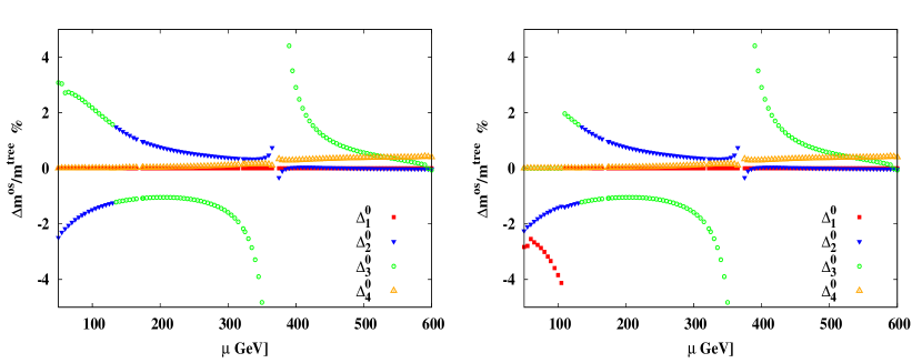
                              (a)                                                                   (b)

Figure 1: Radiative corrections (in %) to all the neutralino masses against $\mu$. The masses of two charginos and one neutralino have been used as inputs. Frame (a) is for scheme 1a, where the mass of the lightest neutralino is used as input, whereas frame (b) is for scheme 1b, where instead the mass of the most bino–like neutralino is used as input.

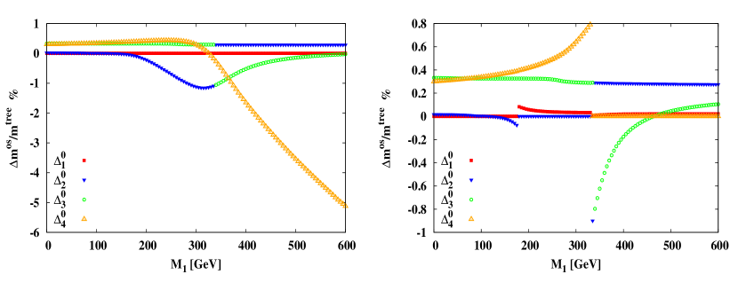
                              (a)                                                                   (b)

Figure 2: Radiative corrections (in %) to all the neutralino masses against $M_{1}$. Frame (a) is for scheme 1a, and frame (b) is for scheme 1b. Note that the two frames employ different scales along the $y-$axis.

In Figure 1 we plot the corrections to the neutralino masses in scheme 1 against $\mu$, with the left (right) frame corresponding to scheme 1a (1b). Both frames show singularities at $\mu=M_{2}$. The reason is that, in these schemes, the expressions for $\delta M_{2}$ and $\delta\mu$ are undefined at $M_{2}=|\mu|$, because $\delta M_{2}$ and $\delta\mu$ are proportional to $\left(M_{2}^{2}-\mu^{2}\right)^{-1}$ [14, 15]. Hence the renormalized masses are undefined if $M_{2}=|\mu|$. Moreover, some corrections remain relatively large as long as $M_{2}$ and $|\mu|$ are close to each other. In particular, the mass of $\tilde{\chi}_{3}^{0}$, which is mostly higgsino–like in this region, receives a large correction, mostly from $\delta\mu$. This pole is rather broad, e.g. $\Delta^{0}_{3}$ can exceed $20\%$ if $\left||\mu|-M_{2}\right|\leq 5$ GeV.

Figs. 1 also show discontinuities at $\mu\simeq 131.50$ GeV. Here a level crossing occurs, i.e. the absolute value of the negative eigenvalue of the neutralino mass matrix $M^{\rm n}$, which used to give $m_{\tilde{\chi}_{3}^{0}}$, decreases past a positive eigenvalue of $M^{\rm n}$ to give $m_{\tilde{\chi}_{2}^{0}}$. However, if we track the corrections corresponding to the negative eigenvalue, there is no discontinuity. A similar situation is encountered for $\mu\sim-100$ GeV, which is not shown in our plots.

With this set of parameters, schemes 1a and 1b perform equally well, i.e. the corrections have similar magnitudes. The results are different for $|\mu|\leq M_{1}$, when the lightest neutralino is no longer bino–like. This leads to another discontinuity in scheme 1b at $\mu\simeq 110$ GeV: for smaller (larger) $\mu$ the most bino–like neutralino is $\tilde{\chi}_{3}^{0}\ (\tilde{\chi}_{1}^{0})$. When approaching this point from above, $\Delta^{0}_{3}$ therefore switches from a positive value to zero, while $\Delta^{0}_{1}$ becomes non–vanishing (and negative, for this choice of parameters). Moreover, $\delta M_{1}$ becomes large in scheme 1a if $|\mu|\ll M_{1}$, as anticipated in the discussion in Subsec.2.3; see also Table 1. This leads to a sizable correction to the mass of the bino–like neutralino.

This does not cause serious instability in Fig. 1, since the small value of $M_{1}$ chosen implies that $\left|M_{1}-\mu\right|$ cannot exceed $M_{Z}$, i.e. $\tilde{\chi}_{1}^{0}$ retains a significant bino component for all values of $\mu$ shown. Note also that LEP searches for $\tilde{\chi}_{1}^{+}\tilde{\chi}_{1}^{-}$ and $\tilde{\chi}_{1}^{0}\tilde{\chi}_{2}^{0}$ production anyway exclude the region $\mu\leq 120$ GeV. The problematic behavior of scheme 1a for $|\mu|<M_{1}-M_{Z}$ becomes more evident in Fig. 2, where we vary $M_{1}$ instead of $\mu$. As $M_{1}$ grows large, the bino component of the lightest neutralino decreases, $N_{11}\propto M_{Z}/(M_{1}-\mu)$. Hence $\delta M_{1}$ becomes large in scheme 1a, giving a large correction to the mass of the bino–like neutralino, which is $\tilde{\chi}_{4}^{0}$ for $M_{1}>M_{2}$ in this figure. Note that in anomaly–mediated supersymmetry breaking one expects $M_{1}\simeq 2.8M_{2}$ [5]. As a consequence $|M_{1}|-|\mu|>M_{Z}$ can easily be realized in such a scenario.

Fig. 2 shows some discontinuities at $M_{1}\simeq 335$ GeV. Just below this value $\tilde{\chi}_{2}^{0}$ is the most bino–like neutralino, but at $M_{1}=335$ GeV $\tilde{\chi}_{4}^{0}$ becomes more bino–like. Shortly thereafter, at $M_{1}\simeq 340$ GeV, there is a level crossing between $\tilde{\chi}_{2}^{0}$ and $\tilde{\chi}_{3}^{0}$; the corresponding eigenvalues of the neutralino mass matrix have opposite sign. Note that all corrections remain below 1% in magnitude near these discontinuities.

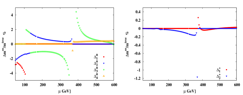
                              (a)                                                                   (b)

Figure 3: Radiative corrections (in %) to (a) the neutralino masses and (b) the chargino masses against $\mu$. Results are for scheme 2b, where the masses of the higgsino–like chargino and of the wino– and bino–like neutralinos are used as inputs.

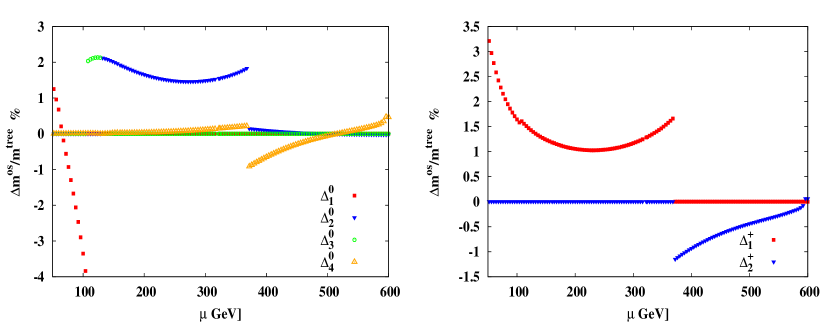
                              (a)                                                                   (b)

Figure 4: Radiative corrections (in %) to (a) the neutralino masses and (b) the chargino masses against $\mu$. Results are for scheme 2c, where the masses of the wino–like chargino and of the bino– and higgsino–like neutralinos are used as inputs.

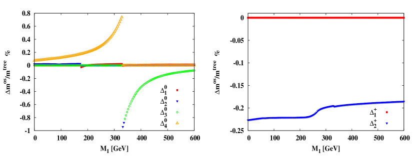
                              (a)                                                                   (b)

Figure 5: Radiative corrections (in %) to (a) the neutralino masses and (b) the chargino masses against $M_{1}$. Results are for scheme 2c, where the masses of the wino–like chargino, bino– and higgsino–like neutralinos are used as inputs.

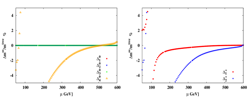
                              (a)                                                                   (b)

Figure 6: Radiative corrections (in %) to (a) the neutralino masses and (b) the chargino masses against $\mu$. Results are for scheme 3a, where the masses of the lightest three neutralinos are used as inputs.

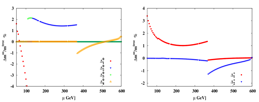
                              (a)                                                                   (b)

Figure 7: Radiative corrections (in %) to (a) the neutralino masses and (b) the chargino masses against $\mu$. Results are for scheme 3b, where the masses of the bino–, wino– and higgsino–like neutralinos are used as inputs.

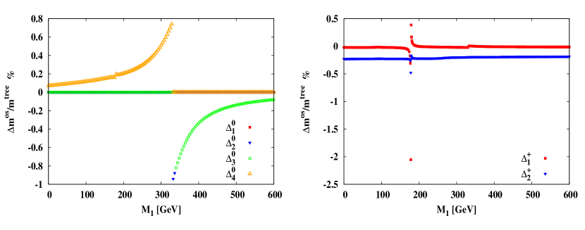
                              (a)                                                                   (b)

Figure 8: Radiative corrections (in %) to (a) the neutralino masses and (b) the chargino masses against $M_{1}$. Results are for scheme 3b, where the masses of the bino–, wino– and higgsino–like neutralinos are used as inputs.

In Fig. 3, we demonstrate that scheme 2b also performs equally well with our choice of parameters. However, the counterterms again show a singularity at $M_{2}\simeq|\mu|$ (although not exactly at $M_{2}=|\mu|$), where the denominator $D$ of the counterterms, given in Eq.(26), vanishes. This again leads to large corrections to the mass of the higgsino–like neutralino $\tilde{\chi}_{3}^{0}$ in the vicinity of the singularity, very similar to both versions of scheme 1.

In contrast, we find that scheme 2a (not shown) performs poorly whenever $M_{2}$ and $|\mu|$ are very different, as anticipated in the discussion of Table 1. In fact, numerically it is considerably worse than scheme 1a. In the latter only $\delta M_{1}$ is occasionally poorly determined; the corresponding corrections are determined by the $U(1)_{Y}$ coupling. In scheme 2a, $\delta\mu$ or $\delta M_{2}$ can be poorly determined, which receive corrections proportional to the larger $SU(2)$ coupling. As a result the region of parameter space with large corrections is not only larger in scheme 2a than in scheme 1a, the size of the correction in these regions also tends to be larger.

Scheme 2c does not have any singularity near $M_{2}=|\mu|$. In Fig. 4 it produces stable and small corrections to all three chargino and neutralino masses that are not inputs for the entire range of $\mu$. The curves in this figure show several discontinuities, but these are harmless, since they do not endanger perturbative stability. In particular, in frame (a) we observe the same discontinuity as in Fig. 1, since the states $\tilde{\chi}_{3}^{0}$ and $\tilde{\chi}_{2}^{0}$ cross each other at this point. The discontinuities at $\mu\simeq 110$ GeV have the same origin as in scheme 1b, see the discussion of Fig. 1(b). Finally, at $\mu\simeq 370$ GeV (i.e. $M_{2}\simeq\mu$), the wino–like state changes from $\tilde{\chi}_{2}^{+}$ to $\tilde{\chi}_{1}^{+}$ as $\mu$ increases. This affects $\delta M_{2}$ significantly, giving rise to (harmless) discontinuities in both frames of Fig. 4.

In Fig. 5 we illustrate results for scheme 2c as function of $M_{1}$. The discontinuities in the corrections to neutralino masses near $M_{1}=335$ GeV have the same origin as in scheme 1b, see Fig. 2(b). All corrections are well behaved for $|M_{1}|\simeq|\mu|$.

Fig. 6 demonstrates that scheme 3a also behaves poorly. For $\mu\>\raisebox{-2.15277pt}{$\stackrel{{\scriptstyle\textstyle<}}{{\sim}}$}\>200$ GeV all three input states, which are the lightest three neutralinos in this scheme, have small wino component. As a consequence the $\delta M_{2}$ is poorly determined, leading to huge corrections to the masses of the wino–like states $\tilde{\chi}_{4}^{0}$ and $\tilde{\chi}_{2}^{+}$, largely from $\delta M_{2}$. The scheme also shows instability around $M_{1}=\mu$, giving very large corrections to the masses of both charginos and the wino–like neutralino.

Scheme 3b does not have any singularity near $M_{2}=|\mu|$. In Fig. 7, like scheme 2c, it also produces stable and small corrections to all three chargino and neutralino masses that are not inputs for the entire range of $\mu$. In frame (a) we observe the same discontinuity as in Fig. 1, since the states $\tilde{\chi}_{3}^{0}$ and $\tilde{\chi}_{2}^{0}$ cross each other at this point. The discontinuities at $\mu\simeq 110$ GeV have the same origin as in scheme 1b, see the discussion of Fig. 1(b). The harmless discontinuities at $\mu\simeq 370$ GeV (i.e. $M_{2}\simeq\mu$), are essentially the same as in Fig. 4.

In Fig. 8 we show results for scheme 3b as function of $M_{1}$. The discontinuities in the corrections to neutralino masses near $M_{1}=335$ GeV have the same origin as in scheme 1b, see Fig. 2(b). In the case at hand this also leads to a small discontinuity in $\Delta_{1}^{+}$. All corrections are well behaved for $|M_{1}|\simeq|\mu|$, but there is some instability around $M_{1}=178.14$ GeV. Here the denominator $D$, given in Eq.(33), of the counterterms vanishes. As a result, the neutralino and chargino masses become ill–defined at this point. The effect of this pole is most visible in the mass of the lightest chargino which, being wino–like, receives dominant correction from $\delta M_{2}$. However, even this corrections drops to $\sim 2\%$ when $M_{1}$ is just $1$ GeV away from the pole, i.e. this pole is much narrower than the poles at $M_{2}=|\mu|$ in schemes 1a and 1b, and the poles at $M_{2}\simeq|\mu|$ in schemes 2a and 2b. These poles are discussed in more detail in the following Subsection.

4.2 Singularities in the Counterterms

                              (a)                                                                   (b)

Figure 9: Contours of constant radiative corrections to (a) the higgsino–like neutralino mass around $M_{2}\simeq\mu$ in scheme 1b, (b) the wino–like chargino mass around $M_{1}\sim M_{2}$ in scheme 3b have been plotted against $\mu$ and $M_{1}$ respectively. Only corrections exceeding $10\%$ have been shown. The patch in (b), at $M_{1}\sim 300$ GeV, is actually at $M_{1}\sim-300$ GeV, i.e. it is plotted against $-M_{1}$.

In Fig. 9 the occurrence of poles, i.e. true divergences in the “finite” parts of the counterterms (as opposed to harmless discontinuities due to level crossings and the like), is analyzed further. These are not due to divergent loop integrals, but due to zeroes of the denominators in the expressions for the counterterms [Eqs.(26) and (33), and the corresponding expression for scheme 1]. We have assumed $M_{1}=180$ GeV and $\mu=300$ GeV in Figs. 9a and 9b, respectively. Here we show the maximal (relative) corrections. In scheme 1b these occur for the higgsino–like neutralino, i.e. Fig. 9a shows $\Delta_{2}^{0}$ (for $\mu\>\raisebox{-2.15277pt}{$\stackrel{{\scriptstyle\textstyle<}}{{\sim}}$}\>168$ GeV as well as $168\ {\rm GeV}\>\raisebox{-2.15277pt}{$\stackrel{{\scriptstyle\textstyle<}}{{\sim}}$}\>\mu\>\raisebox{-2.15277pt}{$\stackrel{{\scriptstyle\textstyle<}}{{\sim}}$}\>174\ {\rm GeV}$ and $M_{2}>\mu$) or $\Delta_{3}^{0}$ (for $\mu\>\raisebox{-2.15277pt}{$\stackrel{{\scriptstyle\textstyle>}}{{\sim}}$}\>174$ GeV as well as $168\ {\rm GeV}\>\raisebox{-2.15277pt}{$\stackrel{{\scriptstyle\textstyle<}}{{\sim}}$}\>\mu\>\raisebox{-2.15277pt}{$\stackrel{{\scriptstyle\textstyle<}}{{\sim}}$}\>174\ {\rm GeV}$ and $M_{2}<\mu$). In scheme 3b the mass of the wino–like chargino instead receives the largest correction, i.e. Fig. 9b, shows $\Delta_{2}^{+}$ (for $M_{2}>\mu$) or $\Delta^{+}_{1}$ (for $M_{2}<\mu$). Finally, scheme 2b shows instability both at $M_{2}\simeq|\mu|$ and at $M_{1}\simeq M_{2}$.

As already mentioned, it is easy to see that $\delta M_{2}$ and $\delta\mu$ diverge in both versions of scheme 1 at $M_{2}=|\mu|$ [14, 15]. In schemes 2 and 3 the expressions for the denominators of the counterterms, given in Eqs.(26) and (33), respectively, are too complicated to allow the derivation of analytical expressions for the pole positions in terms of the input parameters $M_{1},\,M_{2},\,\mu$ and $\tan\beta$. However, it is easy to see that in the limit of small mixing only one term in each of these expressions is large, leading to non–vanishing (and sizable) denominators. Cancellations leading to poles can only occur in the presence of large mixing, which requires at least one of the differences $\left||M_{1}|-M_{2}\right|,\ \left||M_{1}|-|\mu|\right|,\ \left|M_{2}-|\mu|\right|$ to be relatively small. Note that this is a necessary condition, not a sufficient one.

In fact, Eqs.(26) and (33) show that singularities can only occur if at least two of the input states are strongly mixed. This explains the absence of poles at $M_{2}\simeq|\mu|$ in schemes 2c and 3b. Here the most higgsino–like neutralino is chosen as input state. Note that even at $M_{2}=|\mu|$ only one of the two higgsino–like neutralinos mixes strongly with the wino; the other state corresponds to an eigenvalue with opposite sign ($\simeq-|\mu|$), and shows little mixing. Small mixing means large higgsino component, i.e. this weakly mixed state is picked up by our algorithm as the most higgsino–like one. At $M_{2}=|\mu|$ (and sufficiently large $\left||M_{1}|-M_{2}\right|$) the input states in these schemes are thus a relatively pure bino (neutralino), a relatively pure higgsino (neutralino), and a strongly mixed wino–higgsino state (a chargino in scheme 2c, a neutralino in scheme 3b). The fact that two input states show little mixing is sufficient to single out one term in eqs.(26) and (33) as dominant one, making significant cancellations impossible. A similar argument explains why none of our schemes has instabilities for $|M_{1}|\simeq|\mu|$ (unless one also has $M_{2}\simeq|\mu|$; see below).

Scheme 3b shows a singularity at $M_{1}\simeq M_{2}$ where two input neutralino states are strong mixtures of the bino and wino current states, leading to a cancellation between the last two terms in Eq.(33) with all other terms being small. Note that the pole occurs only when $|M_{1}-|\mu||>|M_{2}-|\mu||$. We did not find any pole if $|M_{1}-\mu|\lesssim 80$ GeV. In this interval one of the bino–wino mixed states (usually the more wino–like one) also has a substantial higgsino component, and correspondingly reduced gaugino components. Thus there are no longer two input states with very similar bino and wino components.

This pole at $M_{1}\simeq M_{2}$ is very narrow. This is partly due to cancellations of the numerators of the expressions for the counterterms, which can be understood as follows. Near the pole, indices $i$ and $j$ denote strong mixtures between bino and wino states, and $k$ denotes a higgsino state with little mixing (unless $\left||\mu|-M_{2}\right|$ is also small). In that case only two terms in each of Eqs.(34)–(36) are not suppressed. These terms are antisymmetric in $i\leftrightarrow j$, hence strong mixing also induces strong cancellations; however, these cancellations are not perfect, since mixing pushes the masses $m_{\tilde{\chi}_{i}^{0}}$ and $m_{\tilde{\chi}_{j}^{0}}$ apart.

The finite parts of the counterterms themselves can therefore become quite large, often exceeding the tree–level values of these parameters. Even then corrections to physical masses need not be large, due to cancellations in Eqs.(15) and (16). By construction these cancellations are perfect for the three input states. If an output state is of similar nature as one of the input states, there will then also be strong cancellations for the mass of this output state. For example, in scheme 1b with $M_{2}\simeq|\mu|$, the strong wino–higgsino mixtures in the neutralino sector have similar wino and higgsino components as the two input chargino states, leading to strong cancellations. The largest correction then results for the (almost) unmixed higgsino state in the neutralino sector, as shown in Fig. 9a. The same argument explains why in the “generic” situation with relatively small mixing, in all our b and c schemes the mass of the most strongly mixed state will receive the largest correction, since it is most different from all the input states, which are the least mixed ones in these schemes.

In scheme 3b with $M_{1}\simeq M_{2}$, both strongly mixed gaugino–like neutralinos, which are the cause of the pole, are input states, and hence have perfect cancellations. These states mix relatively weakly with the higgsino–like states. The counterterm $\delta\mu$, which diverges at the pole, comes with coefficient $-2N_{k3}^{*}N_{k4}^{*}$ in Eq.(16). In the limit of vanishing higgsino–gaugino mixing, this is the same for the two higgsino–like states, one having $N_{k3}\simeq N_{k4}\simeq i/\sqrt{2}$ (purely imaginary), while the other had $N_{k3}\simeq-N_{k4}=1/\sqrt{2}$ (purely real, but with opposite signs). This explains why the correction to the mass of the single output state in the neutralino sector remains very small near this pole, see Fig. 8.

One of the two chargino states is also higgsino–like, and the cancellation will go through. However, the second chargino is wino–like. Since there is no wino–like neutralino, only strongly mixed ones, the cancellation in the equation for the mass of this wino–like chargino is quite incomplete. This explains why this state receives the largest correction, as shown in Fig. 9b.

The cancellations we discussed so far work (to some extent) near all poles, and help to confine their effects to quite narrow strips of parameter space, as shown in Fig. 9. The fact that the instability region of scheme 3b at $M_{1}\simeq M_{2}$ is much narrower than that of scheme 1b (or 2b) at $M_{2}\simeq|\mu|$ is due to the fact that wino–bino mixing, which causes the former, only occurs at second order in an expansion of the neutralino masses and eigenstates in powers of $M_{Z}$, while wino–higgsino mixing, which causes the latter, already occurs at first order; wino–bino mixing is also suppressed by an extra factor of $\sin\theta_{W}$. As a result, significant wino–bino mixing occurs over a much smaller region of parameter space than large wino–higgsino mixing.

Finally, if $-M_{1}\simeq M_{2}\simeq|\mu|$ there are two bino–higgsino mixed states and two wino–higgsino mixed states in the neutralino sector. Thus scheme 3b also suffers from instability around this point because two input states are strongly mixed. This explains the patch in Fig. 9b at $M_{1}\sim-300$ GeV. Note that here the “finite” parts of the counterterms diverge only in a very small region in the $(M_{1},M_{2})$ plane, extending for about 1 MeV in $M_{2}$ and about 300 MeV in $M_{1}$; this instability is thus qualitatively different from the one at $M_{1}\simeq M_{2}$, where a pole occurs along a line that is unbounded towards large $M_{2}$.

The singularity at $M_{1}\simeq M_{2}$ does not exist in scheme 2c, since in this scheme again only one of the three input states, the most bino–like neutralino, is strongly mixed in this region of parameter space. The input chargino state is mostly wino–like, unless one in addition has $M_{2}\simeq|\mu|$, and the second input neutralino is again mostly higgsino (even if $M_{2}\simeq|\mu|$, as explained above).

For fixed $\mu$ and $\tan\beta$ Scheme 2c can therefore at worst become singular in a very narrow patch in the $(M_{1},M_{2})$ plane, in the region $-M_{1}\simeq M_{2}\simeq|\mu|$. We saw above that this leads to two bino–higgsino mixed states and two wino–higgsino mixed states in the neutralino sector. The chargino sector also contains two strongly mixed (wino–higgsino) states. Note that the denominator $D$ of Eq.(26) is not a continuous function of the input parameters, since the indices $i,j,k$ defining the input states take different values in different regions of parameter space. This makes it rather difficult to systematically search for zeroes of this denominator. A straightforward numerical scan of $M_{1}$ and $M_{2}$ with step size of $0.01$ GeV did not find any evidence for a zero of the denominator. We did find points with large (finite parts of) $\delta M_{1},\,\delta M_{2}$ and $\delta\mu$ in a very narrow region of parameter space, similar to the patch in Fig. 9b. However, even in that region the renormalized masses remain well behaved in scheme 2c, the maximal correction not exceeding $4\%$. This is due to the two types of cancellation discussed above. Note that all our other schemes lead to considerable larger corrections around this point. We thus conclude that scheme 2c is the most stable of the seven schemes we investigated.

4.3 Comparison Between Schemes

It is generally expected that the physical masses calculated using two different renormalization schemes at one–loop level can differ only by terms of two–loop order. In the case at hand this is true whenever the schemes are well behaved. We demonstrate this explicitly by comparing results for schemes 1b and 3b. We then show another example where this no longer holds, since one of the schemes produces large corrections close to one of the singularities discussed in the previous Subsection. We do not discuss schemes 1a, 2a and 3a in this Subsection, since we already saw that they perform poorly in large regions of parameter space, see Table 1.

We use the following “tree level” parameters to calculate the on–shell renormalized masses in scheme (1b):

$$\text{Set~{}A:}~{}~{}M_{1}=90~{}\text{GeV},~{}M_{2}=200~{}\text{GeV},~{}\mu=300~{}\text{GeV},~{}\tan\beta=5.$$

The masses thus obtained are shown in column 3 of Table 2. We then take $m_{\tilde{\chi}_{1}^{0}}$, $m_{\tilde{\chi}_{2}^{0}}$ and $m_{\tilde{\chi}_{3}^{0}}$, thus obtained, as input masses for scheme 3b. Note that these are respectively the masses of the most bino–, wino– and higgsino–like neutralino. From these three masses, we compute numerically $M_{1}$, $M_{2}$ and $\mu$:

$$\text{Set~{}B:}~{}~{}M_{1}=89.9697~{}\text{GeV},~{}M_{2}=199.7935~{}\text{GeV},~{}\mu=301.0052~{}\text{GeV},~{}\tan\beta=5.$$

We then calculate the one–loop masses in scheme 3b. The resulting spectrum is shown in column 4 of Table 2. We also list in parentheses the one–loop masses calculated using parameter set A within scheme 3b. As shown in column 5, the differences between the two one–loop predictions, using scheme 1b with Set A and scheme 3b with set B, are much smaller than the differences between tree–level and one–loop corrections (except for the input masses, of course, where the latter differences vanish). This is a non–trivial check of our calculation.

Note that using the same numerical values for $M_{1},\,M_{2}$ and $\mu$ in both schemes leads to differences between one–loop masses that are themselves of one–loop order, as shown by the numbers in parentheses in column 5 of Table 2. Only after fixing three physical masses to be the same in both schemes do the predictions for all other masses become nearly identical. The reason is that $M_{1},\,M_{2}$ and $\mu$ are themselves scheme dependent quantities.

Particle	$m^{\rm tree}_{\tilde{\chi}}\ [{\rm GeV}]$	$m^{\rm 1-loop,\,os}_{\tilde{\chi}}\ [{\rm GeV}]$		$\delta m_{\tilde{\chi}}\ [{\rm GeV}]$
	[set A]	scheme 1b	scheme 3b	col. (3) -col. (4)
		[set A]	[set B (set A)]
$\tilde{\chi}_{1}^{+}$	$170.4007$	$170.4007$	$170.4030~{}(170.3714)$	$-0.0023~{}(0.0293)$
$\tilde{\chi}_{2}^{+}$	$337.5026$	$337.5026$	$337.5169~{}(336.7472)$	$-0.0143~{}(0.7554)$
$\tilde{\chi}_{1}^{0}$	$84.8425$	$84.8425$	$84.8425~{}(84.8425)$	$0.0~{}(0.0)$
$\tilde{\chi}_{2}^{0}$	$172.1478$	$172.1545$	$172.1545~{}(172.1478)$	$0.0~{}(0.0067)$
$\tilde{\chi}_{3}^{0}$	$305.4830$	$306.4778$	$306.4778~{}(305.4830)$	$0.0~{}(0.9948)$
$\tilde{\chi}_{4}^{0}$	$338.4927$	$339.6138$	$339.6313~{}(338.8642)$	$-0.0175~{}(0.7496)$

Table 2: Masses of the charginos and neutralinos. The second column lists tree–level predictions for input set A. Columns 3 and 4 list one–loop predictions for schemes 1b and 3b; in the latter case, the first entry is for input set B, which has been chosen such that $m_{\tilde{\chi}_{1}^{0}},\,m_{\tilde{\chi}_{2}^{0}}$ and $m_{\tilde{\chi}_{3}^{0}}$ have the same values as in scheme 1b (third column), whereas the numbers in parentheses use input set A. The last column is the difference between the third and fourth columns.

However, as mentioned before, scheme 1b is undefined when $M_{2}=|\mu|$. We also saw that for $M_{2}\simeq|\mu|$ the finite part of the counterterm $\delta\mu$ remains large, so that the mass of a higgsino–like neutralino receives a large correction. This pole is absent in scheme 3b. As a consequence, for the same set of physical masses, the one–loop masses in these two schemes can be quite different. In Table 3 we demonstrate this by explicit computation.

We use the following tree level parameters to calculate the on–shell renormalized masses in scheme 1b:

$$\text{Set~{}C:}~{}~{}M_{1}=90~{}\text{GeV},M_{2}=350~{}\text{GeV},\mu=355~{}\text{GeV},\tan\beta=5.$$

The resulting physical masses are given in column 3 of table (3). Note the very large correction ($>50$ GeV) to $m_{\tilde{\chi}_{3}^{0}}$. As before, we then take $m_{\tilde{\chi}_{1}^{0}}$, $m_{\tilde{\chi}_{0}^{2}}$ and $m_{\tilde{\chi}_{3}^{0}}$, thus obtained, as input masses for scheme 3b. These are respectively the masses of the bino–, wino– and higgsino–like neutralino. From these three masses, we compute numerically $M_{1}$, $M_{2}$ and $\mu$:

$$\text{Set~{}D:}~{}~{}M_{1}=89.2056~{}\text{GeV},~{}M_{2}=319.1479~{}\text{GeV},~{}\mu=418.1529~{}\text{GeV},~{}\tan\beta=5.$$

Note that $\mu$ had to be increased by more than 60 GeV in order to reproduce the one–loop prediction for $m_{\tilde{\chi}_{3}^{0}}$ from scheme 1b. This increase of $\mu$ would also have led to sizable increases of $m_{\tilde{\chi}_{1}^{+}}$ and $m_{\tilde{\chi}_{2}^{0}}$, had we not simultaneously reduced $M_{2}$ by more than 30 GeV. Only $M_{1}$ retains approximately the same value in both Sets.

Particle	$m^{\rm tree}_{\tilde{\chi}}\ [{\rm GeV}]$	$m^{\rm 1-loop,\,os}_{\tilde{\chi}}\ [{\rm GeV}]$		$\delta m_{\tilde{\chi}}\ [{\rm GeV}]$
	[set C]	scheme 1b	scheme 3b	col. (3) -col. (4)
		[set C]	[set D (set C)]
$\tilde{\chi}_{1}^{+}$	$288.3284$	$288.3284$	$288.0337~{}(287.9178)$	$0.2947~{}(0.4106)$
$\tilde{\chi}_{2}^{+}$	$422.2986$	$422.2986$	$452.4840~{}(417.3805)$	$-30.1854~{}(4.9181)$
$\tilde{\chi}_{1}^{0}$	$86.3675$	$86.3675$	$86.3675~{}(86.3675)$	$0.0~{}(0.0)$
$\tilde{\chi}_{2}^{0}$	$289.8939$	$288.7260$	$288.7260~{}(289.8939)$	$0.0~{}(-1.1679)$
$\tilde{\chi}_{3}^{0}$	$359.1238$	$421.9883$	$421.9883~{}(359.1238)$	$0.0~{}(62.8645)$
$\tilde{\chi}_{4}^{0}$	$422.8623$	$424.2374$	$454.7079~{}(418.8926)$	$-30.4705~{}(5.3448)$

Table 3: Masses of neutralinos and charginos. The meaning of the various entries is as in Table 2, except that parameter sets A and B have been replaced by sets C and D, respectively.

The resulting one–loop masses in scheme 3b are listed in column 4 of Table 3. In parentheses we also give the one–loop masses calculated using parameter set C using scheme 3b. Column 5 shows that the differences between the one–loop predictions for $m_{\tilde{\chi}_{2}^{+}}$ and $m_{\tilde{\chi}_{4}^{0}}$ are very large. This is due to the large differences in the input parameters between Set C and Set D, which in turn was enforced by the large correction to $m_{\tilde{\chi}_{3}^{0}}$ in scheme 1b.

We emphasize that in the case at hand, the predictions of scheme 1b are clearly not reliable, due to the vicinity of the pole at $M_{2}=\mu$ which leads to a breakdown of the perturbative expansion in this scheme. In scheme 3b the differences between tree–level and one–loop masses do not exceed 1% for both set C and set D. Moreover, differences between physical masses are again very small if scheme 3b is compared to scheme 2c, which also has no pole at $M_{2}\simeq\mu$.

5 Conclusion

In this paper we have analyzed variants of the on–shell renormalization of the chargino and neutralino sector of the MSSM. There are six physical particles with in general different masses in this sector, but only three free parameters whose counterterms are determined from this sector. Hence only three masses can be chosen as “input masses”, which by definition are unchanged to all orders in perturbation theory; the remaining three masses will receive quantum corrections, which we computed to one–loop order.

We introduced seven different versions of the on–shell scheme in Sec. 2. These schemes differ by the states whose masses are used as inputs. General considerations led us to expect that all schemes where the indices of the three input states are fixed a priori can show instability over large regions of parameter space, as listed in Table 1 for schemes 1a, 2a and 3a; we confirmed this by explicit calculations in Subsec. 4.1. In these regions at least one of three counterterms $\delta M_{1},\,\delta M_{2}$ and $\delta\mu$ is poorly determined, since none of the input masses is very sensitive to it. These large regions of instability can be avoided by choosing the masses one bino–like, one wino–like and one higgsino–like state as input; the definition of these states, and other practical matters, have been discussed in Sec. 3. This ensures that there is at least one input mass that is sensitive to each counterterm.

Unfortunately this is not sufficient to avoid all regions of instability. In particular, we see that all schemes where the mass of the higgsino–like chargino is used as an input become unstable for $M_{2}\simeq|\mu|$, because finite parts of the counterterms $\delta M_{2}$ and $\delta\mu$ become very large, leading to a very large correction to the mass of the (most) higgsino–like neutralino. This instability is caused by numerical cancellations in the denominators of the expressions for the counterterms, which can only occur if at least two input states are strongly mixed states. We saw in Subsecs. 4.2 and 4.3 that this instability can lead to a collapse of the perturbative expansion over a significant region of parameter space. It can be avoided if instead the mass of the higgsino–like neutralino is used as input; this state does not mix strongly even if $M_{2}\simeq|\mu|$ or $|M_{1}|\simeq|\mu|$.

Finally, we found another similar pole, with however in general much smaller numerical values of the corrections somewhat away from the pole, if the masses of both the bino– and wino–like neutralino are used as inputs. This instability is due to bino–wino mixing, which occurs at $M_{1}\simeq M_{2}$. It can be avoided by chosing the mass of the wino–like chargino, rather than the wino–like neutralino, as input, since the charginos are obviously not affected by bino–wino mixing.

We conclude that the perturbatively most stable version of the on–shell scheme is the one where the masses of the wino–like chargino, and of the bino– and higgsino–like neutralinos are used as inputs; the scheme where the masses of the bino–, wino– and higgsino–like neutralinos are used as input performs as well over most, but not all, of parameter space.

We emphasize that a poor choice of renormalization scheme can lead to unphysically large corrections not only to some masses, but also to cross sections. For example, the exchange of heavier neutralino states can play an important role in the cross section for the annihilation of a pair of the lightest neutralinos into final states containing gauge and/or Higgs bosons [38]; the total neutralino annihilation cross section determines their present relic density if they are stable. The proper choice of renormalization scheme should therefore be important for a variety of one–loop calculations in the MSSM that have been, and are being, performed.

Acknowledgment

We would like to thank Thomas Hahn and Karina Williams for helping with the installation of the Feyn packages, and Nicolas Bernal for help with Gnuplot. This work was partially supported by the DFG Transregio TR33 “The Dark Side of the Universe”, and partly by the German Bundesministerium für Bildung und Forschung (BMBF) under Contract No. 05HT6PDA.

Appendix A

Here we give expressions for $\delta M_{1}$, $\delta M_{2}$ and $\delta\mu$ in terms of the $\delta m_{\tilde{\chi}}$ of Eq.(12) as well as the counterterms to the off–diagonal entries of the chargino and neutralino mass matrices, which can be derived from Eqs.(2.2) and (18). These expressions have been obtained by solving equations (2.3), i.e. they are valid for all versions of scheme 2, with different variants corresponding to different choices of the indices $i,j,k$ (see Table 1). The counterterms can be written as

$$\delta M_{1} = \dfrac{N_{M_{1}}}{D},$$ (23)

$$\delta M_{2} = \dfrac{N_{M_{2}}}{D},$$ (24)

$$\delta\mu = \dfrac{N_{\mu}}{2D},$$ (25)

where

$$D=2N^{*}_{i3}N^{*}_{i4}N^{*^{2}}_{j1}U^{*}_{k1}V^{*}_{k1}-2N^{*^{2}}_{i1}N^{*}_{j3}N^{*}_{j4}U^{*}_{k1}V^{*}_{k1}+N^{*^{2}}_{i2}N^{*^{2}}_{j1}U^{*}_{k2}V^{*}_{k2}-N^{*^{2}}_{i1}N^{*^{2}}_{j2}U^{*}_{k2}V_{k2},$$ (26)

$$N_{\mu}=-\left((\delta m_{\tilde{\chi}^{0}_{i}}-2\delta M^{n}_{i3}N^{*}_{i1}N^{*}_{i3}-2\delta M^{n}_{23}N^{*}_{i2}N^{*}_{i3}-2\delta M^{n}_{14}N^{*}_{i1}N^{*}_{i4}\right.$$ (27)

$$\left.-2\delta M^{n}_{24}N^{*}_{i2}N^{*}_{i4})N^{*^{2}}_{j1}+N^{*^{2}}_{i1}(-\delta m_{\tilde{\chi}^{0}_{j}}+2\delta M^{n}_{13}N^{*}_{j1}N^{*}_{j3}+2\delta M^{n}_{23}N^{*}_{j2}N^{*}_{j3}\right.$$

$$\left.+2\delta M^{n}_{14}N^{*}_{j1}N^{*}_{j4}+2\delta M^{n}_{24}N^{*}_{j2}N^{*}_{j4})\right)U^{*}_{k1}V^{*}_{k1}+\left(-N^{*^{2}}_{i2}N^{*^{2}}_{j1}+N^{*^{2}}_{i1}N^{*^{2}}_{j2}\right)$$

$$\left(-\delta m_{\tilde{\chi}^{+}_{k}}+\delta M^{c}_{21}U^{*}_{k2}V^{*}_{k1}+\delta M^{c}_{12}U^{*}_{k1}V^{*}_{k2}\right),$$

$$N_{M_{2}} = 2\delta m_{\tilde{\chi}^{+}_{k}}N^{*}_{i3}N^{*}_{i4}N^{*^{2}}_{j1}-2\delta m_{\tilde{\chi}^{+}_{k}}N^{*^{2}}_{i1}N^{*}_{j3}N^{*}_{j4}-2\delta M^{c}_{21}N^{*}_{i3}N^{*}_{i4}N^{*^{2}}_{j1}U^{*}_{k2}V^{*}_{k1}$$ (28)

$$+ 2\delta M^{c}_{21}N^{*^{2}}_{i1}N^{*}_{j3}N^{*}_{j4}U^{*}_{k2}V^{*}_{k1}-2\delta M^{c}_{12}N^{*}_{i3}N^{*}_{i4}N^{*^{2}}_{j1}U^{*}_{k1}V^{*}_{k2}-\delta m_{\tilde{\chi}^{0}_{j}}N^{*^{2}}_{i1}U^{*}_{k2}V^{*}_{k2}$$

$$+ \delta M^{c}_{12}N^{*^{2}}_{i1}N^{*}_{j3}N^{*}_{j4}U^{*}_{k1}V^{*}_{k2}+\delta m_{\tilde{\chi}^{0}_{i}}N^{*^{2}}_{j1}U^{*}_{k2}V^{*}_{k2}-2\delta M^{n}_{13}N^{*}_{i1}N^{*}_{i3}N^{*^{2}}_{j1}U^{*}_{k2}V^{*}_{k2}$$

$$- 2\delta M^{n}_{23}N^{*}_{i2}N^{*}_{i3}N^{*^{2}}_{j1}U^{*}_{k2}V^{*}_{k2}-2\delta M^{n}_{14}N^{*}_{i1}N^{*}_{i4}N^{*^{2}}_{j1}U^{*}_{k2}V^{*}_{k2}-2\delta M^{n}_{24}N^{*}_{i2}N^{*}_{i4}N^{*^{2}}_{j1}U^{*}_{k2}V^{*}_{k2}$$

$$+ 2\delta M^{n}_{13}N^{*^{2}}_{i1}N^{*}_{j1}N^{*}_{j3}U^{*}_{k2}V^{*}_{k2}+2\delta M^{n}_{23}N^{*^{2}}_{i1}N^{*}_{j2}N^{*}_{j3}U^{*}_{k2}V^{*}_{k2}+2\delta M^{n}_{14}N^{*^{2}}_{i1}N^{*}_{j1}N^{*}_{j4}U^{*}_{k2}V^{*}_{k2}$$

$$+ 2\delta M^{n}_{24}N^{*^{2}}_{i1}N^{*}_{j2}N^{*}_{j4}U^{*}_{k2}V^{*}_{k2},$$

$$N_{M_{1}} = 2\delta m_{\tilde{\chi}^{+}_{k}}N^{*}_{i3}N^{*}_{i4}N_{j2}^{*^{2}}-2\delta m_{\tilde{\chi}^{+}_{k}}N_{i2}^{*^{2}}N^{*}_{j3}N^{*}_{j4}-2\delta m_{\tilde{\chi}^{0}_{j}}N^{*}_{i3}N^{*}_{i4}U^{*}_{k1}V^{*}_{k1}-\delta m_{\tilde{\chi}^{0}_{j}}N_{i2}^{*^{2}}U^{*}_{k2}V^{*}_{k2}$$ (29)

$$- 2\delta M^{n}_{14}N^{*}_{i1}N^{*}_{i4}N_{j2}^{*^{2}}U^{*}_{k2}V^{*}_{k2}-2\delta M^{n}_{24}N^{*}_{i2}N^{*}_{i4}N_{j2}^{*^{2}}U^{*}_{k2}V^{*}_{k2}+2\delta M^{n}_{13}N_{i2}^{*^{2}}N^{*}_{j1}N^{*}_{j3}U^{*}_{k2}V^{*}_{k2}$$

$$+ 2\delta M^{n}_{23}N_{i2}^{*^{2}}N^{*}_{j2}N^{*}_{j3}U^{*}_{k2}V^{*}_{k2}+2\delta M^{n}_{14}N_{i2}^{*^{2}}N^{*}_{j1}N^{*}_{j4}U^{*}_{k2}V^{*}_{k2}+2\delta M^{n}_{24}N_{i2}^{*^{2}}N^{*}_{j2}N^{*}_{j4}U^{*}_{k2}V^{*}_{k2}$$

$$- 2\delta M^{c}_{12}N^{*}_{i3}N^{*}_{i4}N_{j2}^{*^{2}}U^{*}_{k1}V^{*}_{k2}+2\delta M^{c}_{12}N_{i2}^{*^{2}}N^{*}_{j3}N^{*}_{j4}U^{*}_{k1}V^{*}_{k2}+4\delta M^{n}_{13}N^{*}_{i3}N^{*}_{i4}N^{*}_{j1}N^{*}_{j3}U^{*}_{k1}V^{*}_{k1}$$

$$+ 4\delta M^{n}_{23}N^{*}_{i3}N^{*}_{i4}N^{*}_{j2}N^{*}_{j3}U^{*}_{k1}V^{*}_{k1}-2\delta M^{n}_{13}N^{*}_{i1}N^{*}_{i3}N_{j2}^{*^{2}}U^{*}_{k2}V^{*}_{k2}-2\delta M^{n}_{23}N^{*}_{i2}N^{*}_{i3}N_{j2}^{*^{2}}U^{*}_{k2}V^{*}_{k2}$$

$$+ 4\delta M^{n}_{14}N^{*}_{i3}N^{*}_{i4}N^{*}_{j1}N^{*}_{j4}U^{*}_{k1}V^{*}_{k1}+4\delta M^{n}_{24}N^{*}_{i3}N^{*}_{i4}N^{*}_{j2}N^{*}_{j4}U^{*}_{k1}V^{*}_{k1}+2\delta m_{\tilde{\chi}^{0}_{i}}N^{*}_{j3}N^{*}_{j4}U^{*}_{k1}V^{*}_{k1}$$

$$- 4\delta M^{n}_{24}N^{*}_{i2}N^{*}_{i4}N^{*}_{j3}N^{*}_{j4}U^{*}_{k1}V^{*}_{k1}-2\delta M^{c}_{21}N^{*}_{i3}N^{*}_{i4}N_{j2}^{*^{2}}U^{*}_{k2}V^{*}_{k1}+2\delta M^{c}_{21}N_{i2}^{*^{2}}N^{*}_{j3}N^{*}_{j4}U^{*}_{k2}V^{*}_{k1}$$

$$- 4\delta M^{n}_{13}N^{*}_{i1}N^{*}_{i3}N^{*}_{j3}N^{*}_{j4}U^{*}_{k1}V^{*}_{k1}-4\delta M^{n}_{23}N^{*}_{i2}N^{*}_{i3}N^{*}_{j3}N^{*}_{j4}U^{*}_{k1}V^{*}_{k1}-4\delta M^{n}_{14}N^{*}_{i1}N^{*}_{i4}N^{*}_{j3}N^{*}_{j4}U^{*}_{k1}V^{*}_{k1}$$

$$+ \delta m_{\tilde{\chi}^{0}_{i}}N_{j2}^{*^{2}}U^{*}_{k2}V^{*}_{k2}.$$

Appendix B

Here we give $\delta M_{1}$, $\delta M_{2}$ and $\delta\mu$ for scheme 3, obtained from solving equations (2.3). Different variants of this scheme correspond to different choices of $i,j,k$ (see Table 1). The counterterms are given by

$$\delta M_{1} = \dfrac{N_{M_{1}}}{D},$$ (30)

$$\delta M_{2} = \dfrac{N_{M_{2}}}{D},$$ (31)

$$\delta\mu = \dfrac{N_{\mu}}{2D},$$ (32)

where,

$$D = (N^{*}_{i3}N^{*}_{i4}N^{*^{2}}_{j2}N^{*^{2}}_{k1}-N^{*^{2}}_{i2}N^{*}_{j3}N^{*}_{j4}N^{*^{2}}_{k1}-N^{*}_{i3}N^{*}_{i4}N^{*^{2}}_{j1}N^{*^{2}}_{k2}+N^{*^{2}}_{i1}N^{*}_{j3}N^{*}_{j4}N^{*^{2}}_{k2}$$ (33)

$$+N^{*^{2}}_{i2}N^{*^{2}}_{j1}N^{*}_{k3}N^{*}_{k4}-N^{*^{2}}_{i1}N^{*^{2}}_{j2}N^{*}_{k3}N^{*}_{k4}),$$

$$N_{\mu} = -\delta m_{\tilde{\chi}^{0}_{k}}N^{*^{2}}_{i2}N^{*^{2}}_{j1}+\delta m_{\tilde{\chi}^{0}_{k}}N^{*^{2}}_{i1}N^{*^{2}}_{j2}+\delta m_{\tilde{\chi}^{0}_{j}}N^{*^{2}}_{i2}N^{*^{2}}_{k1}-\delta m_{\tilde{\chi}^{0}_{i}}N^{*^{2}}_{j2}N^{*^{2}}_{k1}$$ (34)

$$+ 2\delta M^{n}_{13}N^{*}_{i1}N^{*}_{i3}N^{*^{2}}_{j2}N^{*^{2}}_{k1}+2\delta M^{n}_{23}N^{*}_{i2}N^{*}_{i3}N^{*^{2}}_{j2}N^{*^{2}}_{k1}+2\delta M^{n}_{14}N^{*}_{i1}N^{*}_{i4}N^{*^{2}}_{j2}N^{*^{2}}_{k1}$$

$$+ 2\delta M^{n}_{24}N^{*}_{i2}N^{*}_{i4}N^{*}_{j2}N^{*^{2}}_{k1}-2\delta M^{n}_{13}N^{*^{2}}_{i2}N^{*}_{j1}N^{*}_{j3}N^{*^{2}}_{k1}-2\delta M^{n}_{23}N^{*^{2}}_{i2}N^{*}_{j2}N^{*}_{j3}N^{*^{2}}_{k1}$$

$$- 2\delta M^{n}_{14}N^{*^{2}}_{i2}N^{*}_{j1}N^{*}_{j4}N^{*^{2}}_{k1}-2\delta M^{n}_{24}N^{*^{2}}_{i2}N^{*}_{j2}N^{*}_{j4}N^{*^{2}}_{k1}-\delta m_{\tilde{\chi}^{0}_{j}}N^{*^{2}}_{i1}N^{*^{2}}_{k2}+\delta m_{\tilde{\chi}^{0}_{i}}N^{*^{2}}_{j1}N^{*^{2}}_{k2}$$

$$- 2\delta M^{n}_{13}N^{*}_{i1}N^{*}_{i3}N^{*^{2}}_{j1}N^{*^{2}}_{k2}-2\delta M^{n}_{23}N^{*}_{i2}N^{*}_{i3}N^{*^{2}}_{j1}N^{*^{2}}_{k2}-2\delta M^{n}_{14}N^{*}_{i1}N^{*}_{i4}N^{*^{2}}_{j1}N^{*^{2}}_{k2}$$

$$- 2\delta M^{n}_{24}N^{*}_{i2}N^{*}_{i4}N^{*^{2}}_{j1}N^{*^{2}}_{k2}+2\delta M^{n}_{13}N^{*^{2}}_{i1}N^{*}_{j1}N^{*}_{j3}N^{*^{2}}_{k2}+2\delta M^{n}_{23}N^{*^{2}}_{i1}N^{*}_{j2}N^{*}_{j3}N^{*^{2}}_{k2}$$

$$+ 2\delta M^{n}_{14}N^{*^{2}}_{i1}N^{*}_{j1}N^{*}_{j4}N^{*^{2}}_{k2}+2\delta M^{n}_{24}N^{*^{2}}_{i1}N^{*}_{j2}N^{*}_{j4}N^{*^{2}}_{k2}+2\delta M^{n}_{13}N^{*^{2}}_{i2}N^{*^{2}}_{j1}N^{*}_{k1}N^{*}_{k3}$$

$$- 2\delta M^{n}_{13}N^{*^{2}}_{i1}N^{*^{2}}_{j2}N^{*}_{k1}N^{*}_{k3}+2\delta M^{n}_{23}N^{*^{2}}_{i2}N^{*^{2}}_{j1}N^{*}_{k2}N^{*}_{k3}-2\delta M^{n}_{23}N^{*^{2}}_{i1}N^{*^{2}}_{j2}N^{*}_{k2}N^{*}_{k3}$$

$$+ 2\delta M^{n}_{14}N^{*^{2}}_{i2}N^{*^{2}}_{j1}N^{*}_{k1}N^{*}_{k4}-2\delta M^{n}_{14}N^{*^{2}}_{i1}N^{*^{2}}_{j2}N^{*}_{k1}N^{*}_{k4}+2\delta M^{n}_{24}N^{*^{2}}_{i2}N^{*^{2}}_{j1}N^{*}_{k2}N^{*}_{k4}$$

$$- 2\delta M^{n}_{24}N^{*^{2}}_{i1}N^{*^{2}}_{j2}N^{*}_{k2}N^{*}_{k4},$$

$$N_{M_{2}} = -\delta m_{\tilde{\chi}^{0}_{k}}N^{*}_{i3}N^{*}_{i4}N^{*^{2}}_{j1}+\delta m_{\tilde{\chi}^{0}_{k}}N^{*^{2}}_{i1}N^{*}_{j3}N^{*}_{j4}+\delta m_{\tilde{\chi}^{0}_{j}}N^{*}_{i3}N^{*}_{i4}N^{*^{2}}_{k1}+\delta m_{\tilde{\chi}^{0}_{i}}N^{*^{2}}_{j1}N^{*}_{k3}N^{*}_{k4}$$ (35)

$$- 2\delta M^{n}_{13}N^{*}_{i3}N^{*}_{i4}N^{*}_{j1}N^{*}_{j3}N^{*^{2}}_{k1}-2\delta M^{n}_{23}N^{*}_{i3}N^{*}_{i4}N^{*}_{j2}N^{*}_{j3}N^{*^{2}}_{k1}-2\delta M^{n}_{14}N^{*}_{i3}N^{*}_{i4}N^{*}_{j1}N^{*}_{j4}N^{*^{2}}_{k1}$$

$$- 2\delta M^{n}_{24}N^{*}_{i3}N^{*}_{i4}N^{*}_{j2}N^{*}_{j4}N^{*^{2}}_{k1}-\delta m_{\tilde{\chi}^{0}_{i}}N^{*}_{j3}N^{*}_{j4}N^{*^{2}}_{k1}+2\delta M^{n}_{13}N^{*}_{i1}N^{*}_{i3}N^{*}_{j3}N^{*}_{j4}N^{*^{2}}_{k1}$$

$$+ 2\delta M^{n}_{23}N^{*}_{i2}N^{*}_{i3}N^{*}_{j3}N^{*}_{j4}N^{*^{2}}_{k1}+2\delta M^{n}_{14}N^{*}_{i1}N^{*}_{i4}N^{*}_{j3}N^{*}_{j4}N^{*^{2}}_{k1}+2\delta M^{n}_{24}N^{*}_{i2}N^{*}_{i4}N^{*}_{j3}N^{*}_{j4}N^{*^{2}}_{k1}$$

$$+ 2\delta M^{n}_{13}N^{*}_{i3}N^{*}_{i4}N^{*^{2}}_{j1}N^{*}_{k1}N^{*}_{k3}-2\delta M^{n}_{13}N^{*^{2}}_{i1}N^{*}_{j3}N^{*}_{j4}N^{*}_{k1}N^{*}_{k3}+2\delta M^{n}_{23}N^{*}_{i3}N^{*}_{i4}N^{*^{2}}_{j1}N^{*}_{k2}N^{*}_{k3}$$

$$- 2\delta M^{n}_{23}N^{*^{2}}_{i1}N^{*}_{j3}N^{*}_{j4}N^{*}_{k2}N^{*}_{k3}+2\delta M^{n}_{14}N^{*}_{i3}N^{*}_{i4}N^{*^{2}}_{j1}N^{*}_{k1}N^{*}_{k4}-2\delta M^{n}_{14}N^{*^{2}}_{i1}N^{*}_{j3}N^{*}_{j4}N^{*}_{k1}N^{*}_{k4}$$

$$+ 2\delta M^{n}_{24}N^{*}_{i3}N^{*}_{i4}N^{*^{2}}_{j1}N^{*}_{k2}N^{*}_{k4}-2\delta M^{n}_{24}N^{*^{2}}_{i1}N^{*}_{j3}N^{*}_{j4}N^{*}_{k2}N^{*}_{k4}-\delta m_{\tilde{\chi}^{0}_{j}}N^{*^{2}}_{i1}N^{*}_{k3}N^{*}_{k4}$$

$$- 2\delta M^{n}_{13}N^{*}_{i1}N^{*}_{i3}N^{*^{2}}_{j1}N^{*}_{k3}N^{*}_{k4}-2\delta M^{n}_{23}N^{*}_{i2}N^{*}_{i3}N^{*^{2}}_{j1}N^{*}_{k3}N^{*}_{k4}-2\delta M^{n}_{14}N^{*}_{i1}N^{*}_{i4}N^{*^{2}}_{j1}N^{*}_{k3}N^{*}_{k4}$$

$$- 2\delta M^{n}_{24}N^{*}_{i2}N^{*}_{i4}N^{*^{2}}_{j1}N^{*}_{k3}N^{*}_{k4}+2\delta M^{n}_{13}N^{*^{2}}_{i1}N^{*}_{j1}N^{*}_{j3}N^{*}_{k3}N^{*}_{k4}+2\delta M^{n}_{23}N^{*^{2}}_{i1}N^{*}_{j2}N^{*}_{j3}N^{*}_{k3}N^{*}_{k4}$$

$$+ 2\delta M^{n}_{14}N^{*^{2}}_{i1}N^{*}_{j1}N^{*}_{j4}N^{*}_{k3}N^{*}_{k4}+2\delta M^{n}_{24}N^{*^{2}}_{i1}N^{*}_{j2}N^{*}_{j4}N^{*}_{k3}N^{*}_{k4},$$

and,

$$N_{M_{1}} = \delta m_{\tilde{\chi}^{0}_{k}}N^{*}_{i3}N^{*}_{i4}N^{*^{2}}_{j2}-\delta m_{\tilde{\chi}^{0}_{k}}N^{*^{2}}_{i2}N^{*}_{j3}N^{*}_{j4}-\delta m_{\tilde{\chi}^{0}_{j}}N^{*}_{i3}N^{*}_{i4}N^{*^{2}}_{k2}+2\delta M^{n}_{13}N^{*}_{i3}N^{*}_{i4}N^{*}_{j1}N^{*}_{j3}N^{*^{2}}_{k2}$$ (36)

$$+ 2\delta M^{n}_{23}N^{*}_{i3}N^{*}_{i4}N^{*}_{j2}N^{*}_{j3}N^{*^{2}}_{k2}+2\delta M^{n}_{14}N^{*}_{i3}N^{*}_{i4}N^{*}_{j1}N^{*}_{j4}N^{*^{2}}_{k2}+2\delta M^{n}_{24}N^{*}_{i3}N^{*}_{i4}N^{*}_{j2}N^{*}_{j4}N^{*^{2}}_{k2}$$

$$+ \delta m_{\tilde{\chi}^{0}_{i}}N^{*}_{j3}N^{*}_{j4}N^{*^{2}}_{k2}-2\delta M^{n}_{13}N^{*}_{i1}N^{*}_{i3}N^{*}_{j3}N^{*}_{j4}N^{*^{2}}_{k2}-2\delta M^{n}_{23}N^{*}_{i2}N^{*}_{i3}N^{*}_{j3}N^{*}_{j4}N^{*^{2}}_{k2}$$

$$- 2\delta M^{n}_{14}N^{*}_{i1}N^{*}_{i4}N^{*}_{j3}N^{*}_{j4}N^{*^{2}}_{k2}-2\delta M^{n}_{24}N^{*}_{i2}N^{*}_{i4}N^{*}_{j3}N^{*}_{j4}N^{*^{2}}_{k2}-2\delta M^{n}_{13}N^{*}_{i3}N^{*}_{i4}N^{*^{2}}_{j2}N^{*}_{k1}N^{*}_{k3}$$

$$+ 2\delta M^{n}_{13}N^{*^{2}}_{i2}N^{*}_{j3}N^{*}_{j4}N^{*}_{k1}N^{*}_{k3}-2\delta M^{n}_{23}N^{*}_{i3}N^{*}_{i4}N^{*^{2}}_{j2}N^{*}_{k2}N^{*}_{k3}+2\delta M^{n}_{23}N^{*^{2}}_{i2}N^{*}_{j3}N^{*}_{j4}N^{*}_{k2}N^{*}_{k3}$$

$$- 2\delta M^{n}_{14}N^{*}_{i3}N^{*}_{i4}N^{*^{2}}_{j2}N^{*}_{k1}N^{*}_{k4}+2\delta M^{n}_{14}N^{*^{2}}_{i2}N^{*}_{j3}N^{*}_{j4}N^{*}_{k1}N^{*}_{k4}-2\delta M^{n}_{24}N^{*}_{i3}N^{*}_{i4}N^{*^{2}}_{j2}N^{*}_{k2}N^{*}_{k4}$$

$$+ 2\delta M^{n}_{24}N^{*^{2}}_{i2}N^{*}_{j3}N^{*}_{j4}N^{*}_{k2}N^{*}_{k4}+\delta m_{\tilde{\chi}^{0}_{j}}N^{*^{2}}_{i2}N^{*}_{k3}N^{*}_{k4}-\delta m_{\tilde{\chi}^{0}_{i}}N^{*^{2}}_{j2}N^{*}_{k3}N^{*}_{k4}$$

$$+ 2\delta M^{n}_{13}N^{*}_{i1}N^{*}_{i3}N^{*^{2}}_{j2}N^{*}_{k3}N^{*}_{k4}+2\delta M^{n}_{23}N^{*}_{i2}N^{*}_{i3}N^{*^{2}}_{j2}N^{*}_{k3}N^{*}_{k4}+2\delta M^{n}_{14}N^{*}_{i1}N^{*}_{i4}N^{*^{2}}_{j2}N^{*}_{k3}N^{*}_{k4}$$

$$+ 2\delta M^{n}_{24}N^{*}_{i2}N^{*}_{i4}N^{*^{2}}_{j2}N^{*}_{k3}N^{*}_{k4}-2\delta M^{n}_{13}N^{*^{2}}_{i2}N^{*}_{j1}N^{*}_{j3}N^{*}_{k3}N^{*}_{k4}-2\delta M^{n}_{23}N^{*^{2}}_{i2}N^{*}_{j2}N^{*}_{j3}N^{*}_{k3}N^{*}_{k4}$$

$$- 2\delta M^{n}_{14}N^{*^{2}}_{i2}N^{*}_{j1}N^{*}_{j4}N^{*}_{k3}N^{*}_{k4}-2\delta M^{n}_{24}N^{*^{2}}_{i2}N^{*}_{j2}N^{*}_{j4}N^{*}_{k3}N^{*}_{k4}.$$

Appendix C

We show by explicit calculation that using the $\tilde{\chi}_{i}^{+}\tilde{\chi}_{i}^{-}Z$ couplings, it is possible to determine which of the two charginos is more wino–like, or, equivalently, whether $M_{2}$ is bigger or smaller than $|\mu|$. The relevant terms we compare are

$$C_{i}=(-V_{i1}^{2}-\dfrac{1}{2}V_{i2}^{2}+s_{W}^{2})^{2}+(-U_{i1}^{2}-\dfrac{1}{2}U_{i2}^{2}+s_{W}^{2})^{2},~{}\forall~{}i\in~{}\{1,2\}\,,$$ (37)

which determine the sum of the squares of the left– and right–handed couplings. These terms contribute, for example, to the chargino pair production cross section through $Z-$boson exchange in the $s-$channel in $e^{+}e^{-}$ or $pp$ collisions. Recall that we use the convention $M_{2}>0$ and assume vanishing CP phases in the chargino mass matrix. However, $\mu$ can be either positive or negative. The unitary mixing matrices $U$ and $V$ are real. They satisfy

$$U_{ii}^{2}=U_{jj}^{2},~{}U_{ij}^{2}=U_{ji}^{2},$$

$$V_{ii}^{2}=V_{jj}^{2},~{}V_{ij}^{2}=V_{ji}^{2},$$ (38)

where $\{i,j\}\in\{1,2\}$.

Recall that, for given $\tan\beta$, we can solve the equations for the physical masses $m_{\tilde{\chi}_{i}^{+}}$ for the parameters $M_{2}$ and $\mu$, with a four–fold ambiguity. Part of this ambiguity is due to the fact that the expressions for the physical masses are invariant under the exchange of $M_{2}$ and $\mu$. Here we show that the quantities $C_{i}$ of Eq.(37) can be used to resolve this ambiguity. We show this separately for positive and negative $\mu$.

• $case~{}1:$ $\mu>0$
  Let $a,b$ be the possible solutions for $M_{2},\mu$; $a,b>0$. For $\{M_{2},\mu\}=\{a,b\}$, let $\mathcal{U}$ and $\mathcal{V}$ be the unitary mixing matrices satisfying Eq.(4). Then, for $\{M_{2},\mu\}=\{b,a\}$, the corresponding matrices are given by $\mathcal{VO}$ and $\mathcal{UO}$ respectively, where

  $$\cal{O}=\left(\begin{array}[]{cc}0&1\\ 1&0\end{array}\right).$$ (39)

  Using relations (Appendix C), it is straightforward to observe that in $M^{c}$, $a\leftrightarrow b$ corresponds to $C_{1}\leftrightarrow C_{2}$.

• $case~{}2:$ $\mu<0$
  Let $a,b$ be the possible solutions for $M_{2},|\mu|$; $a,b>0$. For $\{M_{2},\mu\}=\{a,-b\}$, let $\mathcal{U}$ and $\mathcal{V}$ be the unitary mixing matrices satisfying Eq.(4). Then, for $\{M_{2},\mu\}=\{b,-a\}$, the corresponding matrices are given by $\mathcal{V\tilde{O}}$ and $\mathcal{U\tilde{O}}^{T}$ respectively, where

  $$\cal{\tilde{O}}=\left(\begin{array}[]{cc}0&1\\ -1&0\end{array}\right).$$ (40)

  Again, $\{a,-b\}\leftrightarrow\{b,-a\}$ corresponds to $C_{1}\leftrightarrow C_{2}$.

We thus see that by comparing $C_{1}$ with $C_{2}$ it is possible in both cases to determine the ordering of $M_{2}$ and $|\mu|$. However, if $M_{2}\simeq|\mu|$, it can be difficult to infer whether $M_{2}>|\mu|$ or vice versa. This is of some importance, since precisely in this region of parameter space schemes where the mass of the more higgsino–like chargino is used as input show an instability, as we saw in Sec. 4.

References

- [1] E. Witten, “Dynamical Breaking of Supersymmetry,” Nucl.Phys. B188 (1981) 513.
- [2] N. Sakai, “Naturalness in Supersymmetric Guts,” Z.Phys. C11 (1981) 153.
- [3] S. Dimopoulos and H. Georgi, “Softly Broken Supersymmetry and SU(5),” Nucl.Phys. B193 (1981) 150.
- [4] R. K. Kaul and P. Majumdar, “Cancellation of quadratically divergent mass corrections in globally supersymmetric sponteneously broken gauge theories,” Nucl.Phys. B199 (1982) 36.
- [5] M. Drees, R. Godbole, and P. Roy, “Theory and phenomenology of sparticles: An account of four-dimensional N=1 supersymmetry in high energy physics,”. Hackensack, USA: World Scientific (2004) 555 p.
- [6] H. Baer and X. Tata, “Weak scale supersymmetry: From superfields to scattering events,”.
- [7] A. Collab., “ATLAS Detector and Physics Performance Technical Design Report,”.
- [8] T. L. S. Group, “Physics Interplay of the LHC and the ILC,” arXiv:hep-ph/0410364.
- [9] R. Keisler, C. Reichardt, K. Aird, B. Benson, L. Bleem, et al., “A Measurement of the Damping Tail of the Cosmic Microwave Background Power Spectrum with the South Pole Telescope,” arXiv:1105.3182 [astro-ph.CO]. * Temporary entry *.
- [10] T. Fritzsche and W. Hollik, “Complete one-loop corrections to the mass spectrum of charginos and neutralinos in the MSSM,” Eur. Phys. J. C24 (2002) 619–629, arXiv:hep-ph/0203159.
- [11] W. Oller, H. Eberl, W. Majerotto, and C. Weber, “Analysis of the chargino and neutralino mass parameters at one-loop level,” Eur. Phys. J. C29 (2003) 563–572, arXiv:hep-ph/0304006.
- [12] H. Eberl, M. Kincel, W. Majerotto, and Y. Yamada, “One-loop corrections to the chargino and neutralino mass matrices in the on-shell scheme,” Phys. Rev. D64 (2001) 115013, arXiv:hep-ph/0104109.
- [13] M. Drees, W. Hollik, and Q. Xu, “One-loop calculations of the decay of the next-to-lightest neutralino in the MSSM,” JHEP 02 (2007) 032, arXiv:hep-ph/0610267.
- [14] J. Guasch, W. Hollik, and J. Sola, “Fermionic decays of sfermions: A complete discussion at one-loop order,” JHEP 10 (2002) 040, arXiv:hep-ph/0207364.
- [15] N. Baro and F. Boudjema, “Automatised full one-loop renormalisation of the MSSM II: The chargino-neutralino sector, the sfermion sector and some applications,” Phys. Rev. D80 (2009) 076010, arXiv:0906.1665 [hep-ph].
- [16] T. Ibrahim and P. Nath, “The neutron and the lepton EDMs in MSSM, large CP violating phases, and the cancellation mechanism,” Phys. Rev. D58 (1998) 111301, arXiv:hep-ph/9807501.
- [17] M. Pospelov and A. Ritz, “Electric dipole moments as probes of new physics,” Annals Phys. 318 (2005) 119–169, arXiv:hep-ph/0504231.
- [18] Particle Data Group Collaboration, K. Nakamura et al., “Review of particle physics,” J.Phys.G G37 (2010) 075021.
- [19] H. K. Dreiner, S. Heinemeyer, O. Kittel, U. Langenfeld, A. M. Weber, et al., “Mass Bounds on a Very Light Neutralino,” Eur.Phys.J. C62 (2009) 547–572, arXiv:0901.3485 [hep-ph].
- [20] W. Marciano and A. Sirlin, “Radiative Corrections to Neutrino Induced Neutral Current Phenomena in the SU(2)-L x U(1) Theory,” Phys.Rev. D22 (1980) 2695.
- [21] P. H. Chankowski, S. Pokorski, and J. Rosiek, “Complete on-shell renormalization scheme for the minimal supersymmetric Higgs sector,” Nucl. Phys. B423 (1994) 437–496, arXiv:hep-ph/9303309.
- [22] A. Dabelstein, “The One loop renormalization of the MSSM Higgs sector and its application to the neutral scalar Higgs masses,” Z. Phys. C67 (1995) 495–512, arXiv:hep-ph/9409375.
- [23] K. Desch, J. Kalinowski, G. A. Moortgat-Pick, M. Nojiri, and G. Polesello, “SUSY parameter determination in combined analyses at LHC / LC,” JHEP 0402 (2004) 035, arXiv:hep-ph/0312069 [hep-ph].
- [24] D. M. Pierce, J. A. Bagger, K. T. Matchev, and R.-j. Zhang, “Precision corrections in the minimal supersymmetric standard model,” Nucl.Phys. B491 (1997) 3–67, arXiv:hep-ph/9606211 [hep-ph].
- [25] H. Baer, F. E. Paige, S. D. Protopopescu, and X. Tata, “ISAJET 7.81: A Monte Carlo Event Generator for p p, pbar p, and e+ e- Interactions, http://www.nhn.ou.edu/ isajet/,”.
- [26] A. Djouadi, J.-L. Kneur, and G. Moultaka, “SuSpect: A Fortran code for the supersymmetric and Higgs particle spectrum in the MSSM,” Comput.Phys.Commun. 176 (2007) 426–455, arXiv:hep-ph/0211331 [hep-ph].
- [27] B. Allanach, “SOFTSUSY: a program for calculating supersymmetric spectra,” Comput.Phys.Commun. 143 (2002) 305–331, arXiv:hep-ph/0104145 [hep-ph].
- [28] W. Porod, “SPheno, a program for calculating supersymmetric spectra, SUSY particle decays and SUSY particle production at e+ e- colliders,” Comput.Phys.Commun. 153 (2003) 275–315, arXiv:hep-ph/0301101 [hep-ph].
- [29] P. Z. Skands, B. Allanach, H. Baer, C. Balazs, G. Belanger, et al., “SUSY Les Houches accord: Interfacing SUSY spectrum calculators, decay packages, and event generators,” JHEP 0407 (2004) 036, arXiv:hep-ph/0311123 [hep-ph].
- [30] B. Allanach, C. Balazs, G. Belanger, M. Bernhardt, F. Boudjema, et al., “SUSY Les Houches Accord 2,” Comput.Phys.Commun. 180 (2009) 8–25, arXiv:0801.0045 [hep-ph].
- [31] J. A. Aguilar-Saavedra, A. Ali, B. C. Allanach, R. L. Arnowitt, H. A. Baer, et al., “Supersymmetry parameter analysis: SPA convention and project,” Eur.Phys.J. C46 (2006) 43–60, arXiv:hep-ph/0511344 [hep-ph].
- [32] T. Hahn, “Generating Feynman diagrams and amplitudes with FeynArts 3,” Comput. Phys. Commun. 140 (2001) 418–431, arXiv:hep-ph/0012260.
- [33] T. Hahn and C. Schappacher, “The implementation of the minimal supersymmetric standard model in FeynArts and FormCalc,” Comput. Phys. Commun. 143 (2002) 54–68, arXiv:hep-ph/0105349.
- [34] T. Hahn and M. Perez-Victoria, “Automatized one-loop calculations in four and D dimensions,” Comput. Phys. Commun. 118 (1999) 153–165, arXiv:hep-ph/9807565.
- [35] T. Hahn and M. Perez-Victoria, “Automatized one-loop calculations in four and D dimensions,” Comput. Phys. Commun. 118 (1999) 153–165, arXiv:hep-ph/9807565.
- [36] F. del Aguila, A. Culatti, R. Munoz Tapia, and M. Perez-Victoria, “Techniques for one-loop calculations in constrained differential renormalization,” Nucl. Phys. B537 (1999) 561–585, arXiv:hep-ph/9806451.
- [37] W. Siegel, “Supersymmetric Dimensional Regularization via Dimensional Reduction,” Phys. Lett. B84 (1979) 193.
- [38] M. Drees and M. M. Nojiri, “The Neutralino relic density in minimal supergravity,” Phys.Rev. D47 (1993) 376–408, arXiv:hep-ph/9207234 [hep-ph].