Capturing correlations in chaotic diffusion by approximation methods

Abstract

We investigate three different methods for systematically approximating the diffusion coefficient of a deterministic random walk on the line which contains dynamical correlations that change irregularly under parameter variation. Capturing these correlations by incorporating higher order terms, all schemes converge to the analytically exact result. Two of these methods are based on expanding the Taylor-Green-Kubo formula for diffusion, whilst the third method approximates Markov partitions and transition matrices by using a slight variation of the escape rate theory of chaotic diffusion. We check the practicability of the different methods by working them out analytically and numerically for a simple one-dimensional map, study their convergence and critically discuss their usefulness in identifying a possible fractal instability of parameter-dependent diffusion, in case of dynamics where exact results for the diffusion coefficient are not available.

I Introduction

Diffusion is a fundamental macroscopic transport process in many-particle systems. It is quantifiable by the diffusion coefficient, which describes the linear growth in the mean-squared displacement of an ensemble of particles. The source of this growth is often considered to be a Brownian or random process of collisions between particles. However, on a microscopic scale the equations governing these collisions in physical systems are deterministic and typically chaotic. By studying diffusion in chaotic dynamical systems we can attempt to take these deterministic rules into account and understand the phenomenon of diffusion from first principles Dorfman (1999); Gaspard (1998); Klages (2007); Cvitanović et al. (2009). Of particular interest is the study of the diffusion coefficient under parameter variation in chaotic dynamical systems such as one-dimensional maps Geisel and Nierwetberg (1982); Schell et al. (1982); Fujisaka and Grossmann (1982); Korabel and Klages (2004), area preserving two dimensional maps Rechester and White (1980); Cary and Meiss (1981); Venegeroles (2007) and particle billiards Machta and Zwanzig (1983); Harayama and Gaspard (2001); Harayama et al. (2002); Mátyás and Klages (2004). Where exact analytical results for chaotic dynamical systems exist Klages (1996); Klages and Dorfman (1995, 1999); Groeneveld and Klages (2002); Cristadoro (2006); Knight and Klages (2011), one finds that the diffusion coefficient is typically a complicated fractal function of control parameters. This phenomenon can be understood as a topological instability of the deterministic diffusive dynamics under parameter variation Klages (1996); Klages and Dorfman (1995, 1999); Klages (2007).

So far exact analytical solutions for the diffusion coefficient could only be derived for simple cases of low-dimensional dynamics. In higher dimensions even very fundamental properties of diffusion coefficients are often unknown, such as whether they are smooth or fractal functions of control parameters Harayama and Gaspard (2001); Jepps and Rondoni (2006); Klages (2007). For example, much effort was spent two decades ago studying more complicated systems like a two-dimensional family of sawtooth maps Cary and Meiss (1981); Dana et al. (1989); Eckhardt (1993). However, despite a good understanding of the orbit structure Percival and Vivaldi (1987a, b) it was not possible to conclude whether the diffusion coefficient is fractal or not Sano (2002). If one wishes to achieve a microscopic understanding of diffusion in more realistic physical systems, one therefore has to rely either on numerical simulations or on approximation methods.

In this paper we compare three different methods for approximating parameter dependent diffusion coefficients with each other by working them out analytically and numerically for a simple one-dimensional map. This model has the big advantage that it is very amenable to rigorous analysis. Its diffusion coefficient has been calculated exactly in Knight and Klages (2011) and was found to be a fractal function of a control parameter. Our goal is to assess the individual capabilities and limitations of these approximation methods in terms of practicability, physical interpretation, convergence towards the exact result, and identification of an underlying fractal structure in the diffusion coefficient. We also address recent criticism by Gilbert and Sanders Gilbert and Sanders (2009), who claimed that one of these methods, as originally proposed in Klages and Korabel (2002), is mathematically wrong and unphysical.

In section II we define the deterministic dynamical system that provides our test case, which is a simple piecewise linear one-dimensional map. In section III the first approximation method is introduced, called correlated random walk in Klages and Korabel (2002), which consists of truncating the Taylor-Green-Kubo formula for diffusion. This method enables us to analytically build up a series of approximations which gives evidence for a fractal structure. In previous work this approximation scheme has successfully been applied to understand parameter dependent diffusion in models that are much more complicated than the one considered here Mátyás and Klages (2004); Korabel and Klages (2004); Harayama et al. (2002); Klages (2007). Motivated by the criticism of Gilbert and Sanders (2009), in this paper we provide further insight into the functioning of this method by working it out rigorously for our specific example. In section IV the persistent random walk method for diffusion is studied. This method was originally proposed within stochastic theory in the form of a persistent random walk Haus and Kehr (1987); Weiss (1994). It consists of approximating the Taylor-Green-Kubo formula by including memory in a self-consistent, persistent way. Recently this method has been worked out for chaotic diffusion in Hamiltonian particle billiards Gilbert and Sanders (2009, 2010); Gilbert et al. (2011). Here we apply this scheme to the different case of a one-dimensional map, and we obtain a series of approximations analytically and then numerically. In section V we look at a third method, defined by a slight variation Klages and Dorfman (1995); Klages (1996); Klages and Dorfman (1999) of the escape rate theory of chaotic diffusion Gaspard and Nicolis (1990); Gaspard and Dorfman (1995); Breymann, Tél, and Vollmer (1996); Gaspard (1998); Dorfman (1999); Vollmer (2002) in that absorbing boundary conditions are replaced by periodic ones. This method thus consists of evaluating the diffusion coefficient in terms of the decay rate of the dynamical system towards the equilibrium state, instead of using the escape rate. The decay rate is in turn obtained by an approximation to the relevant Markov transition matrix. By this method we are able to build up a series of approximations which, through the functional form of the interpolation that we find, gives very strong evidence for fractality. Basic ideas defining this method have been sketched in Klages (2007), however, this is the first time that it has been fully worked out to understand fractal diffusion coefficients. Section VI forms the conclusion.

II A one-dimensional map exhibiting chaotic diffusion

We use the simplest setting possible, where deterministic diffusion is generated by a parameter dependent one-dimensional dynamical system. The equations of motion are determined by a map $M_{h}(x):{\mathbb{R}}\rightarrow{\mathbb{R}}$ so that

$$x_{n+1} = M_{h}(x_{n})$$ (1)

$$= M^{n+1}_{h}(x)\ \ x\in{\mathbb{R}},h\geq 0,n\in{\mathbb{N}},$$

with $x=x_{0}$ Geisel and Nierwetberg (1982); Schell et al. (1982); Fujisaka and Grossmann (1982); Klages and Dorfman (1995). In our case, the map $M_{h}(x)$ is based on the Bernoulli shift or doubling map, combined with a lift parameter $h$, which gives the simple parameter dependent map of the interval

$$M_{h}(x)=\left\{\begin{array}[]{rl}2x+h&0\leq x<\frac{1}{2}\\ 2x-1-h&\frac{1}{2}\leq x<1\end{array}\right..$$ (2)

This map exhibits ‘escape’, i.e., points leave the unit interval under iteration. It is copied and lifted over the real line by

$$M_{h}(x+z)=M_{h}(x)+z,\ \ z\in{\mathbb{Z}}$$ (3)

in order to obtain a map from the real line to itself, see Fig. 1(a). The symmetry in this system ensures that there is no mean drift Groeneveld and Klages (2002). Note that the invariant density of the map Eq. (2) modulo 1 remains by construction simply uniform throughout the whole parameter range. This is in contrast to the related piecewise linear maps studied in Klages (1996); Klages and Dorfman (1995, 1999); Klages (2007), where the density becomes a highly complicated step function under parameter variation, which profoundly simplifies the situation. The model was first introduced in Gaspard and Klages (1998), where its parameter dependent diffusion coefficient $D(h)$ was obtained numerically, while in Gaspard (1992); Dorfman (1999) the diffusion coefficient for a special single parameter value was calculated analytically. Exact analytical solutions for $D(h)$ for all $h\geq 0$ of this and related models were recently obtained in Knight and Klages (2011). Since there is a periodicity with integer values of $h$, here we restrict ourselves to the parameter regime of $h\in[0,1]$ without loss of generality. In Gaspard and Klages (1998); Knight and Klages (2011) it was found that $D(h)$ displays both fractal and linear behaviour, see Fig. 1(b). To our knowledge, this is one of the simplest models that exhibits a fractal diffusion coefficient. Being nevertheless amenable to rigorous analysis, it thus forms a convenient starting point to learn about the power of different approximation methods for understanding complicated diffusion coefficients.

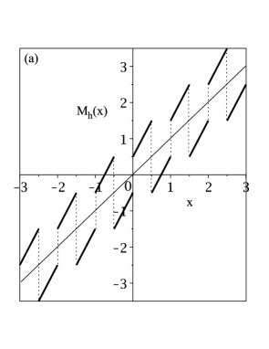
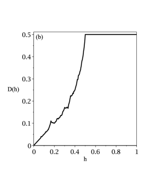
Figure 1: The lifted Bernoulli shift map. A section of the map $M_{h}(x)$, Eqs. (2) and (3), is illustrated in (a) for the value of the control parameter $h=0.5$. The corresponding parameter dependent diffusion coefficient $D(h)$, exactly calculated in Knight and Klages (2011), is shown in (b).

III Correlated random walk

Our first approximation method starts with the diffusion coefficient expressed in terms of the velocity autocorrelation function of the map, called the Taylor-Green-Kubo formula, see Dorfman (1999); Klages and Korabel (2002) for derivations,

$$D(h) = \lim_{n\to\infty}\left(\sum_{k=0}^{n}\int_{0}^{1}v_{0}(x)v_{k}(x)\rho^{*}(x)dx\right)$$ (4)

$$-\frac{1}{2}\int_{0}^{1}v_{0}^{2}(x)\rho^{*}(x)dx\>,$$

where $\rho^{*}(x)$ is the invariant density of the map Eq. (2) modulo 1, this being equal to one throughout the parameter range as we have a family of doubling maps. The velocity function $v_{k}(x)$ calculates the integer displacement of a point at the $k^{th}$ iteration,

$$v_{k}(x)=\left\lfloor x_{k+1}\right\rfloor-\left\lfloor x_{k}\right\rfloor.$$ (5)

In order to create an $n^{th}$ order approximation we simply truncate Eq. (4) at a given $n$ Klages and Korabel (2002). Hence we obtain the finite sum

$$D_{n}(h)=\sum_{k=0}^{n}\int_{0}^{1}v_{0}(x)v_{k}(x)dx-\frac{1}{2}\int_{0}^{1}v^{2}_{0}(x)dx\>,$$ (6)

which can physically be understood as a time dependent diffusion coefficient. Looking at how the sequence of $D_{n}(h)$ converges towards $D(h)$ thus corresponds to incorporating more and more memory in the decay of the velocity autocorrelation function and checking how this decay varies as a function of $h$ for a given $n$. Note that the functional form of $D_{n}(h)$ for finite $n$ is to some extent already determined by our choice of integer displacements in Eq. (5), however, we have checked that for the given model the deviations between using integer and non-integer displacements for finite time are minor. Secondly, we remark that by using this straightforward truncation scheme we have neglected further cross-correlation terms that do not grow linearly in $n$, cf. Dorfman (1999). Still, by definition we have $D_{n}(h)\to D(h)\>(n\to\infty)$. Going to lowest order, for $n=0$ we immediately see that

$$D_{0}(h)=\frac{h}{2}\>,$$ (7)

which is the simple uncorrelated random walk solution for the diffusion coefficient Knight and Klages (2011). In Fig. (2) one can see that $D_{0}(h)$ is asymptotically exact for $h\rightarrow 0$.

Of more interest however are the higher values of $n$ capturing the higher order correlations that come into play. To evaluate these we define a jump function $J^{n}_{h}(x):[0,1]\rightarrow{\mathbb{R}}$,

$$J^{n}_{h}(x)=\sum_{k=0}^{n}v_{k}\left(x\right)\>,$$ (8)

which gives the integer displacement of a point $x$ after $n$ iterations. Equation (8) can be written recursively as Knight and Klages (2011)

$$J^{n}_{h}(x)=v_{0}(x)+J^{n-1}_{h}\left(\tilde{M}_{h}(x)\right),$$ (9)

where $\tilde{M}_{h}(x)$ is Eq. (2) taken modulo $1$. This recursive formula will help when we solve the integral in Eq. (6). Let $T_{h}^{n}(x):[0,1]\rightarrow{\mathbb{R}}$ be defined as

$$T^{n}_{h}(x)=\int_{0}^{x}J^{n}(y)dy,\ \ T^{-1}_{h}(x):=0.$$ (10)

Using Eq. (9) we can solve Eq. (10) recursively as

$$T^{n}_{h}(x)=s_{h}(x)+\frac{1}{2}T^{n-1}\left(\tilde{M}_{h}(x)\right)$$ (11)

with

$$s_{h}(x)=\int_{0}^{x}v_{0}(y)dy=xv_{0}(x)+c,$$ (12)

where the constants of integration $c$ can be evaluated using the continuity of $T_{h}^{n}(x)$ and the fact that $T_{h}^{n}(0)=T_{h}^{n}(1)=0$ as there is no mean drift in this system. We obtain the following functional recursion relation for $T^{n}_{h}(x)$:

$$T_{h}^{n}(x)=\left\{\begin{array}[]{lll}\frac{1}{2}T^{n-1}_{h}(2x+h)&-\frac{1}{2}T_{h}^{n-1}(h)&\ \ 0\leq x<\frac{1-h}{2}\\ \frac{1}{2}T^{n-1}_{h}(2x+h-1)&-\frac{1}{2}T_{h}^{n-1}(h)+x+\left(\frac{h-1}{2}\right)&\ \ \frac{1-h}{2}\leq x<\frac{1}{2}\\ \frac{1}{2}T^{n-1}_{h}(2x-h)&-\frac{1}{2}T_{h}^{n-1}(h)-x+\left(\frac{h+1}{2}\right)&\ \ \frac{1}{2}\leq x<\frac{1+h}{2}\\ \frac{1}{2}T^{n-1}_{h}(2x-1-h)&-\frac{1}{2}T_{h}^{n-1}(h)&\ \ \frac{1+h}{2}\leq x<1\end{array}\right.\ \ .$$ (13)

Using Eq. (13) in Eq. (6) via Eqs. (8) and (10) we can evaluate our $n^{th}$ order approximation as

$$D_{n}(h)=\frac{h}{2}+T_{h}^{n-1}(h).$$ (14)

So we see that the higher order correlations are all captured by the cumulative integral functions $T^{n}_{h}(x)$. In order to evaluate Eq. (14) we construct a recursive relation from Eq. (13),

$$T^{n}_{h}(h)=\sum_{k=0}^{n}\frac{1}{2^{k}}t_{h}\left(\tilde{M}_{h}^{k}(h)\right)-\sum_{k=1}^{n}\frac{1}{2^{k}}T_{h}^{n-k}(h),$$ (15)

where

$$t_{h}(x)=\left\{\begin{array}[]{rl}0&\ \ 0\leq x<\frac{1-h}{2}\\ x+\frac{h-1}{2}&\ \ \frac{1-h}{2}\leq x<\frac{1}{2}\\ -x+\frac{h+1}{2}&\ \ \frac{1}{2}\leq x<\frac{1+h}{2}\\ 0&\ \ \frac{1+h}{2}\leq x<1\end{array}\right.$$ (16)

is $s_{h}(x)$ with the $-\frac{1}{2}T_{h}^{n}(h)$ terms removed. In order to simplify Eq. (15) we write it entirely in terms of Eq. (16). Let

$$\tau_{h}(n)=\sum_{k=1}^{n}\frac{1}{2^{k}}T_{h}^{n-k}(h).$$ (17)

We can write Eq. (17) recursively as

$$\tau_{h}(n)=\frac{1}{2}T_{h}^{n-1}(h)+\frac{1}{2}\tau_{h}(n-1).$$ (18)

Substituting Eqs. (17) and (18) into (15) we obtain

$$T^{n}_{h}(h)=\sum_{k=0}^{n}\frac{1}{2^{k}}t_{h}\left(\tilde{M}_{h}^{k}(h)\right)-\frac{1}{2}T_{h}^{n-1}(h)-\frac{1}{2}\tau_{h}(n-1).$$ (19)

Then substituting Eq. (15) back into Eq. (19)

$$T^{n}_{h}(h)=\sum_{k=0}^{n}\frac{1}{2^{k}}t_{h}\left(\tilde{M}_{h}^{k}(h)\right)-\frac{1}{2}\left(\sum_{k=0}^{n-1}\frac{1}{2^{k}}t_{h}\left(\tilde{M}_{h}^{k}(h)\right)\right)+\frac{1}{2}\tau_{h}(n-1)-\frac{1}{2}\tau_{h}(n-1)$$ (20)

we arrive at our final expression

$$T^{n}_{h}(h)=\frac{1}{2^{n}}t_{h}\left(\tilde{M}_{h}^{n}(h)\right)+\sum_{k=0}^{n-1}\frac{1}{2^{k+1}}t_{h}\left(\tilde{M}_{h}^{k}(h)\right).$$ (21)

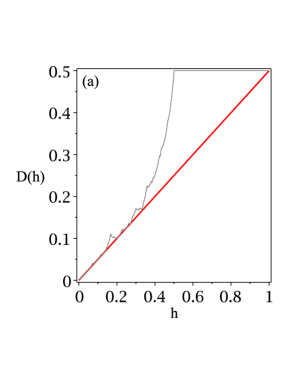
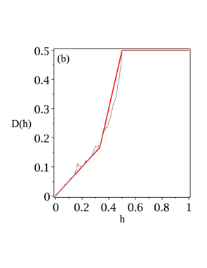
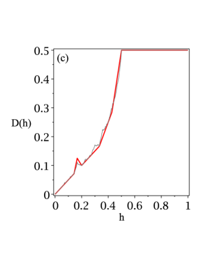
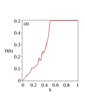
Figure 2: (Colour online) Correlated random walk . In this figure the first four approximations to the parameter dependent diffusion coefficient $D(h)$ are illustrated in bold (red) along with the actual diffusion coefficient. In (a) the zeroth order is shown, which is simply the random walk solution, in (b),(c) and (d) the first, second, and third order approximations, respectively. At each stage one obtains a set of extrema with linear interpolation, which converge quickly to the exact diffusion coefficient $D(h)$. The amount of extrema increases exponentially with $n$, hence we see the fractal structure emerging.

It is helpful to rewrite Eq. (15) in the form of Eq. (21) as it allows us to show that under this method, $D_{n}(h)$ converges exactly to $D(h)$ in finite time for particular values of $h$, see Fig. (2) for an illustration. This means that for a specific set of parameter values, we can fully capture the correlations of the map with a finite time approximation. This convergence is dependent upon the behaviour of the orbit of the point $x=h$ under the map $\tilde{M}_{h}(x)$. In particular, if this orbit is pre-periodic, and the values of the points in the periodic loop correspond to $0$ in Eq. (16), then the time dependent diffusion coefficient $D_{n}(h)$ will converge to the exact value $D(h)$ on the $n^{th}$ step, where $n$ is given by the transient length of the orbit of $h$ plus one. For example, let $h=2/5$,

$$\tilde{M}_{2/5}(2/5) = 1/5$$

$$\tilde{M}_{2/5}(1/5) = 4/5$$

$$\tilde{M}_{2/5}(4/5) = 1/5\>.$$ (22)

So $h=2/5$ is pre-periodic of transient length one. In addition

$$t_{h}(2/5) = 1/10$$

$$t_{h}(1/5) = 0$$

$$t_{h}(4/5) = 0\>,$$ (23)

thus $t_{2/5}\left(\tilde{M}_{2/5}^{n}(2/5)\right)=0$ for $n>1$. Hence we see finite time convergence to $D(h)$. This finite time convergence at a certain set of points is helpful in understanding the structure of $D(h)$ as the fractal diffusion coefficient can be seen emerging around these points in the same manner as an iterated function system like a Koch curve, see Fig. (2).

Being able to analytically expose the fractal structure of parameter dependent diffusion coefficients is the main strength of this method. In addition, the convergence of the series of approximations is very quick due to the finite time convergence at certain values of $h$. Moreover, the fact that one only needs to directly put in the map dynamics makes it very user-friendly. However, due to the recurrence relation that this method is based on, applying it analytically is restricted to one-dimensional systems or higher dimensional systems whose dynamics can be projected down to one-dimensional systems, such as baker maps Gaspard and Klages (1998); Gaspard (1998); Dorfman (1999); Vollmer (2002); Klages (2007). In order to answer questions about more realistic, physical systems, one would need to resort to numerical analysis. By using families of time and parameter dependent diffusion coefficients such as defined by Eq. (6) this is, on the other hand, straightforward, as has been successfully demonstrated for many different types of systems Mátyás and Klages (2004); Korabel and Klages (2004); Harayama et al. (2002); Klages and Korabel (2002); Klages (2007).

This approximation method, represented by Eq. (6), was criticized by Gilbert and Sanders in Gilbert and Sanders (2009) in two ways: First, it was stated that ‘this ad hoc truncation has no physical meaning: if $<v_{0}v_{l}>\neq 0$, it is not true that higher-order correlations $<v_{0}v_{k}>$ vanish’. However, there is no assumption in Eq. (6) that higher-order correlations disappear. On the contrary, this expansion is to be truncated at different time steps for exploring the impact of higher-order correlations on the convergence of the series by systematically incorporating them step by step. Interestingly, as we have shown above, there do exist parameter values for this model at which all higher order correlations disappear. This set, whose number of elements becomes infinite for $n\to\infty$, holds the key to understanding the emergence of the fractal structure in the diffusion coefficient. There is a clear physical interpretation of this set of parameter values in terms of the orbits of the associated critical points of the map, as exemplified above. Under parameter variation these orbits generate complicated sequences of forward and backward scattering, which characterize the diffusive dynamics by physically explaining the origin of the fractal structure in terms of the topological instability of the associated microscopic scattering processes. This physical interpretation, called ‘turnstile dynamics’, has been explained in detail in Klages (1996); Klages and Dorfman (1995, 1999); Klages (2007); Knight and Klages (2011).

Secondly, by applying a higher-dimensional equivalent of Eq. (6) to the billiard models discussed in Gilbert and Sanders (2009) Gilbert and Sanders claimed that in Klages and Korabel (2002) ‘the stationary distribution was erroneously assumed to be uniform’. We first clarify that there is no room for ‘assuming’ any stationary distribution in this equation. The mathematically exact derivation of the Taylor-Green-Kubo formula Eq. (4) is based on time translational invariance of the dynamics, cf. Dorfman (1999); Klages and Korabel (2002), and can only be carried out if the density $\rho^{*}(x)$ in Eq. (6) is strictly the invariant one. Hence, there is no choice, and for our map as well as for the Hamiltonian particle billiards studied in Gilbert and Sanders (2009) this density has to be the invariant one, which in turn for all these systems is uniform. Gilbert and Sanders claim to ‘correct this mistake’ by deriving a second-order approximation of their billiard models which is different from the one obtained from the method outlined in this section as applied to billiards, compare Eq. (11) in Gilbert and Sanders (2009) with Eq. (21) in Klages and Korabel (2002). Their Eq. (11), which they use for their simulations, thus seems to represent a mix between the method outlined in this section and the one described in the following section.

IV Persistent random walk

The next method we look at again starts with the Taylor-Green-Kubo formula for diffusion Eq. (4). However, rather than truncating it, we now approximate the correlations in a more self-consistent way by including memory effects persistently. The key difference to the previous method is that this approach models an exponential decay of the velocity autocorrelation function beyond the lowest order approximation. This method first emerged within stochastic theory as a persistent random walk Haus and Kehr (1987); Weiss (1994) and was recently applied to understand chaotic diffusion in Hamiltonian particle billiards Gilbert and Sanders (2009, 2010); Gilbert et al. (2011).

The main task of evaluating the diffusion coefficient with this method is to find an expression for the correlation function at the $n^{th}$ time step by only including memory effects of a given length. We start by defining the velocity autocorrelation function as a sum over all possible velocities weighted by the corresponding parts of the invariant measure $\mu^{*}$ of the system,

$$\left\langle v_{0}(x)v_{n}(x)\right\rangle=\sum_{v_{0}(x),\ldots,v_{n}(x)}v_{0}(x)v_{n}(x)\mu^{*}(\{v_{0}(x),\ldots,v_{n}(x)\}).$$ (24)

The different parts of the invariant measure in Eq. (24) are approximated by the transition probabilities of the system, depending on the length of memory considered. These in turn are trivially obtained from the invariant probability density function $\rho^{*}(x)$. As a $0^{th}$ order approximation of this method, no memory is considered at all, that is, the movement of a particle is entirely independent of its preceding behaviour. In this case the correlations evaluate simply as

$$\left\langle v_{0}(x)v_{n}(x)\right\rangle=0\ \ (n>0),$$ (25)

thus we need only consider $\left<v^{2}_{0}(x)\right>$. By Eq. (4) the approximate diffusion coefficient is obtained as

$$D_{0}(h)=\frac{1}{2}\int_{0}^{1}\left\langle v^{2}_{0}(x)\right\rangle dx=\frac{h}{2}\>,$$ (26)

which reproduces again the random walk solution, as expected. For the higher order approximations, one must refine the level of memory that is used based upon the microscopic dynamics of the map.

IV.1 One step memory approximation

We now include one step of memory in the system, i.e., we assume that the behaviour of a point at the $n^{th}$ step is only dependent on the $(n-1)^{th}$ step. In Gilbert and Sanders (2009) Eq. (24) was evaluated for approximating the diffusion coefficient in a particle billiard. For this purpose it was assumed that a point moves to a neighbouring lattice point at each iteration. Hence the velocity function $v_{n}(x)$ could only take the values $\ell$ or $-\ell$, where $\ell$ defines the lattice spacing. In order to evaluate the one step memory approximation for the map $M_{h}(x)$, we need to modify the method to include the probability that a point stays at a lattice point and does not move, hence our velocity function can take the values $1,-1$ or $0$. Let $P(b|a)$ be the conditional probability that a point takes the velocity $b$ given that at the previous step it had velocity $a$ with $a,b\in\left\{0,1,-1\right\}$. We use these probabilities to obtain a one step memory approximation. We can write our velocity autocorrelation function as

$$\left\langle v_{0}v_{n}\right\rangle=\sum_{v_{0},...,v_{n}}v_{0}v_{n}p(v_{0})\prod_{i=1}^{n}P(v_{i}|v_{i-1}),$$ (27)

where we let $v_{k}(x)=v_{k}$ for brevities sake and $p(a)$ is the probability that a point takes the velocity $a$ at the first step. We can capture the combinatorics of the sum over all possible paths by rewriting Eq. (27) as a matrix equation,

$$\left\langle v_{0}v_{n}\right\rangle=\left(\begin{array}[]{ccc}0&1&-1\end{array}\right)\left(\begin{array}[]{ccc}P_{00}&P_{01}&P_{0-1}\\ P_{10}&P_{11}&P_{1-1}\\ P_{-10}&P_{-11}&P_{-1-1}\end{array}\right)^{n}\left(\begin{array}[]{c}0\\ p(1)\\ -p(-1)\end{array}\right)$$ (28)

where $P_{ba}=P(b|a)$. Equation (28) can be simplified by using the fact that all the paths with a ‘0’ state cancel each other out, therefore not contributing to diffusion, and by using the symmetries in the system, i.e.,

$$P_{-1-1} = P_{11}$$

$$P_{-11} = P_{1-1}$$

$$p(-1) = p(1)$$ (29)

Hence Eq. (27) can be simplified to

$$\left\langle v_{0}v_{n}\right\rangle=\left(\begin{array}[]{cc}1&-1\end{array}\right)\left(\begin{array}[]{cc}P_{11}&P_{1-1}\\ P_{1-1}&P_{11}\end{array}\right)^{n}\ \left(\begin{array}[]{c}1\\ -1\end{array}\right)p(1),$$ (30)

which is a simple quadratic form. By diagonalisation the expression for the $n^{th}$ velocity autocorrelation function is obtained to

$$\left\langle v_{0}v_{n}\right\rangle=2p(1)\left(P_{11}-P_{1-1}\right)^{n}$$ (31)

yielding the exponential decay of the velocity autocorrelation function $<v_{0}v_{n}>\sim\exp(n\log(P_{11}-P_{1-1}))$ referred to above. Substituting Eq. (31) into the Taylor-Green-Kubo formula Eq. (4) by using the fact that $p(1)=h/2$ gives

$$D(h) = \sum_{n=0}^{\infty}\left\langle v_{0}v_{n}\right\rangle-\frac{1}{2}\left\langle v_{0}^{2}\right\rangle$$ (32)

$$= h\left(\sum_{n=0}^{\infty}\left(P_{11}-P_{1-1}\right)^{n}\right)-\frac{h}{2}$$

$$= \frac{h}{1-P_{11}+P_{1-1}}-\frac{h}{2}.$$

The relevant parameter dependent probabilities can be worked out from the invariant density $\rho^{*}(x)$ of the system and are

$$P_{11}=\left\{\begin{array}[]{ll}0&\ \ 0\leq h<\frac{1}{3}\\ 1-\frac{(1-h)}{2h}&\ \ \frac{1}{3}\leq h<\frac{1}{2}\\ \frac{1}{2}&\ \ \frac{1}{2}\leq h<1\end{array}\right.$$ (33)

and

$$P_{1-1}=\left\{\begin{array}[]{ll}0&\ \ 0\leq h<\frac{1}{3}\\ 0&\ \ \frac{1}{3}\leq h<\frac{1}{2}\\ 1-\frac{1}{2h}&\ \ \frac{1}{2}\leq h<1\end{array}\right.\ \ .$$ (34)

Substituting Eqs. (33) and (34) into Eq. (32) we obtain a persistent one-step memory approximation for the diffusion coefficient of the map $M_{h}(x)$. Figure (3) shows a plot of the final result as a function of the control parameter in comparison to the exact diffusion coefficient $D(h)$.

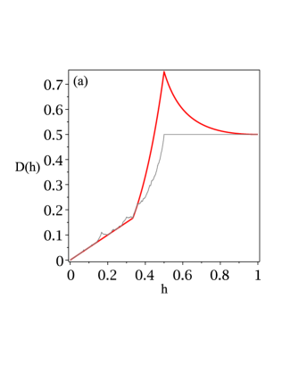
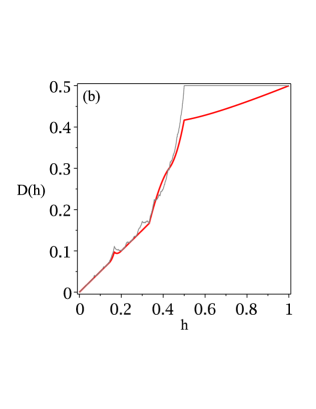
Figure 3: (Colour online) Persistent random walk approximation . In this figure the first order approximation Eq. (32) to the exact parameter dependent diffusion coefficient $D(h)$ is illustrated in (a), the second order Eq. (36) is shown in (b). Approximations are in bold (red) along with the diffusion coefficient. The major topological changes in the dynamics are picked out by piecewise-differentiable approximations.

IV.2 Two step memory approximation

We now extend the approximation to include two steps of memory, i.e., the behaviour of a point at the $n^{th}$ step depends on what has happened at the $(n-1)^{th}$ and $(n-2)^{th}$ step. Let $P(c|b,a)$ be the conditional probability that a point has velocity $c$ given that it had velocity $b$ at the previous step and $a$ at the step before that with $a,b,c\in\left\{0,1,-1\right\}$. For this two step approximation, the velocity autocorrelations are given by

$$\left\langle v_{0}v_{n}\right\rangle=\sum_{v_{0},...,v_{n}}v_{0}v_{n}p(v_{0},v_{1})\prod_{i=2}^{n}P(v_{i}|v_{i-1},v_{i-2}),$$ (35)

where $p(a,b)$ is the probability that a point takes velocity $a$ at the first step followed by $b$. Again we proceed by the method of Gilbert and Sanders (2010) and rewrite Eq. (35) as a matrix equation in order to capture the combinatorics of the sum,

$$\left\langle v_{0}v_{n}\right\rangle=\underline{r}\cdot\underline{\underline{A}}^{n}\cdot\underline{s}$$ (36)

where $\underline{r}$ evaluates $v_{n}$, $\underline{s}$ evaluates $v_{0}p(v_{0},v_{1})$ and $\underline{\underline{A}}$ is the $9\times 9$ probability transition matrix for the system. Unfortunately, Eq. (36) cannot be evaluated analytically (see the Appendix), so we resort to numerical evaluations. The result is depicted in Fig. 3. We see that this method picks out the same topological changes in the map dynamics that the previous method did and interpolates between them, however, the convergence at these points is not as accurate.

The strength of this method is in modeling the exponential decay of correlations that is often found in diffusive systems, particularly in Hamiltonian particle billiards B´alint and Toth (2008). When applied to these systems the method is not restricted by dimension making it very useful in this setting. However, generating by default an exponential decay of correlations is not an ideal approach for diffusive systems in which correlations do not decay exponentially. In contrast to the correlated random walk approach, this method is not designed to reveal possibly fractal structures of parameter dependent diffusion coefficients. It also requires a lot of input about the relevant transition probabilities, making it unpractical when it comes to analysing higher order approximations. In particular, if one was to consider nonhyperbolic systems Korabel and Klages (2004), or even hyperbolic systems with less simple invariant measures Klages and Dorfman (1995); Klages (1996); Klages and Dorfman (1999); Klages and Korabel (2002), then deriving the transition probabilities of Eqs. (33) and (34) would be much more complicated.

V Approximating Markov partitions

The final method that we look at does not involve the Taylor-Green-Kubo formula. Using the framework of the escape rate theory applied to dynamical systems Gaspard and Nicolis (1990); Gaspard and Dorfman (1995); Breymann, Tél, and Vollmer (1996); Gaspard (1998); Dorfman (1999); Vollmer (2002), we consider a truncated map $M_{h}(x)$ defined on $[0,L]$. By applying absorbing boundary conditions to this map, thus generating an open system, standard escape rate theory expresses the diffusion coefficient in terms of the escape rate from a fractal repeller Klages and Dorfman (1999). Here we use a slight variation of this approach by using periodic boundaries. For calculating diffusion coefficients in simple maps this setting is technically easier, because it produces simpler transfer operators than absorbing boundaries Klages (1996). We thus consider a closed system, whose initial density decays exponentially to an invariant one, as quantified by the parameter-dependent decay rate $\gamma_{dec}(h)$. As was shown in Klages (1996); Klages and Dorfman (1995, 1999), by this modified approach, and in complete analogy to ordinary escape rate theory, the diffusion coefficient can be obtained to

$$D(h)=\lim_{L\rightarrow\infty}\frac{L^{2}}{4\pi^{2}}\gamma_{dec}(h).$$ (37)

The decay rate can in turn be calculated exactly if the Frobenius-Perron equation can be mapped onto a Markov transition matrix. In case of $M_{h}(x)$ the second largest eigenvalue $\chi_{1}(h)$ of this transition matrix determines the decay rate according to Klages (1996); Klages and Dorfman (1995, 1999)

$$\gamma_{dec}(h)=ln\left(\frac{2}{\chi_{1}(h)}\right).$$ (38)

Unfortunately, constructing Markov transition matrices exactly for even the simplest parameter dependent maps can be a very complicated task. Our approximate method starts as follows (see Klages (1996); Klages and Dorfman (1999) for details): For a given value of the parameter $h$, we restrict the dynamics to the unit interval by using Eq. (2) modulo $1$. We then consider the set of iterates of the critical point $x=0.5$, which for certain parameter values form a set of Markov partition points. This set is then copied and lifted back onto the system of size $L$ into each unit interval. By supplementing this partition with periodic boundary conditions, it defines a Markov partition for the whole system on $[0,L]$. The key problem is that the behaviour of the orbit of the critical point under parameter variation is very irregular. Therefore we approximate Markov partitions by truncating this orbit for a given parameter value after a certain number of iterations. Typically, the resulting set of points will then not yield a Markov partition for this parameter value. In order to make up for this, we introduce a weighted approximation into our transition matrix to account for any non-Markovian behaviour. For example, if partition part $i$ gets mapped onto a fraction of partition part $j$ then the entry $a_{i,j}$ in the approximate transition matrix will be equal to this fraction; see also Klages (2007) for the basic idea of this approach.

The motivation behind this method is that at each stage of the approximation, whose level is defined by the number of iterates of the critical point, there will be certain values of the parameter whose Markov partitions are exact. So at least for these parameter values we will obtain the precise diffusion coefficient $D(h)$, with interpolations between these points as defined by the approximate transition matrix. That way, we will have full control and understanding over the convergence of our approximations.

We first work out the zeroth order approximation, for which we take the unit intervals as partition parts; see Fig. 4 for an illustration of $M_{h}(x)$ at system size $L=3$. The corresponding approximate transition matrix $\underline{\underline{T}}(h)$ is cyclic and reads

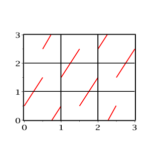
$$\underline{\underline{T}}(h)=\left(\begin{array}[]{ccc}2-2h&h&h\\ h&2-2h&h\\ h&h&2-2h\end{array}\right)\$$

Figure 4: (Colour online) Approximate Markov transition matrix . Illustrated here is the map $M_{h}(x)$ truncated on $[0,L]$ with $L=3$ and periodic boundary conditions. The map is given by the diagonal lines (red) and the zeroth order approximation to the Markov partition is shown by the thick black lines. The partition parts are simply the unit intervals. Note the periodic boundary conditions. The corresponding transition matrix $\underline{\underline{T}}(h)$ is shown below the map. Note that this partition is only Markov when $h=0$ or $1$.

$$\underline{\underline{T}}(h)=\left(\begin{array}[]{ccccc}2-2h&h&0&\ldots&h\\ h&2-2h&h&\ldots&0\\ 0&h&2-2h&h&\ldots\\ \vdots&\vdots&h&\ddots&h\\ h&0&\ldots&h&2-2h\end{array}\right)\>,$$ (39)

therefore the eigenvalues can be evaluated analytically Klages and Dorfman (1995, 1999) as

$$\chi_{1}(h) = 2-2h+2h\cos(2\pi/L)$$ (40)

$$\simeq 2-2h+2h\left(1-\frac{2\pi^{2}}{L^{2}}\right)\>(L\rightarrow\infty)\>.$$

By combining this result with Eq. (38), the decay rate is given as a function of the parameter and length $L$ to

$$\gamma_{dec}(h)=\ln\left(\frac{1}{1-h+h\cos(2\pi/L)}\right)\simeq\frac{h2\pi^{2}}{L^{2}}\>(L\rightarrow\infty).$$ (41)

Using Eq. (41) in Eq. (37), the diffusion coefficient is finally given by

$$D(h)=\frac{h}{2}\>,$$ (42)

which again yields the familiar random walk approximation.

The next stage of approximation involves two partition parts per unit interval, and for this we simply include the critical point $x=0.5$ as a partition point. So our partition parts are the half-unit intervals on the real line. For the next iteration level we include the first iteration of $x=0.5$, $\tilde{M}_{h}(0.5)=1-h$ as a partition point and its mirror image about $x=0.5$ which is $h$, and for each higher approximations we include one more iterate. However, with these higher approximations we no longer obtain a cyclic matrix, so we have to resort to numerics to evaluate the decay rate and the diffusion coefficient. The first three approximations obtained by this method are displayed in Fig. 5.

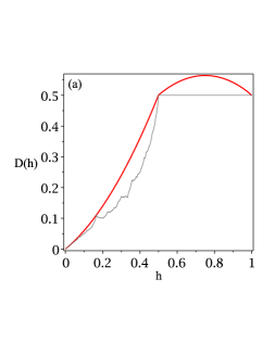
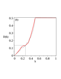
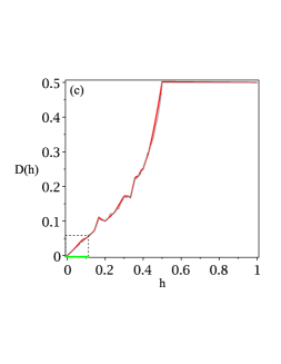
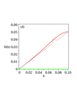
Figure 5: (Colour online) Approximating transition matrices . In this figure, the first order approximation to the parameter dependent diffusion coefficient $D(h)$ obtained by this method is illustrated in (a), and the second and third orders are illustrated in (b) and (c), respectively, whilst a blow up of (c) is shown in (d). The approximations are shown in bold (red) along with the diffusion coefficient diffusion coefficient. We see that the functional form of the interpolation in (a) is repeated in (b) at a smaller scale (see the contents of the dashed line box). This functional form is again repeated on a still smaller scale in (c) as illustrated in (d). This self-similarity provides evidence that the final function $D(h)$ is fractal.

The main strength of this method is that we know by definition where our approximations are going to converge exactly in finite time, namely at Markov partition parameter values $h$ picked out by each subsequent approximation. In addition, the functional form of the interpolation between these points highlights areas of self-similarity and therefore gives one evidence for fractal behaviour even at low-level approximations, see Fig. 5. However, this method quickly relies on numerical computation and again requires considerable input from the user making it unpractical at higher level approximations. It seems unlikely that this method can easily be generalized to higher-dimensional systems, due to the difficulty to construct (approximate) Markov partitions and associated transition matrices.

VI Conclusion

We have studied three different approximation methods applied to a particular chaotic dynamical system. For this model the exact parameter-dependent diffusion coefficient was known beforehand Knight and Klages (2011). Taking it as a reference, the motivation was to learn about the capabilities and the weaknesses of the individual methods. These are of course not a comprehensive list of the many possible ways to approximate the diffusion coefficient of a system, see, for example, Rechester and White (1980); Venegeroles (2007) for diffusion in sawtooth and standard maps. However, what they do illustrate is the fact that even in our simple one-dimensional model studied here, the results that one obtains are very much dependent upon the individual method that one uses, and these results vary greatly between the different methods.

By the first method, which relied on a systematic truncation of the Taylor-Green-Kubo formula, we saw the fractal structure building up fully analytically over a series of correlated random walk approximations, as we were able to exactly capture the correlations of the system in finite time at certain parameter values. This yielded in turn quick convergence to the exact results. Using a persistent random walk approach, the second method retained an exponential decay of correlations even in finite time approximations. However, for the model under consideration this approximation yielded convergence that was significantly weaker than in case of the other two methods. By using a variation of the escape rate approach to chaotic diffusion combined with approximate transition matrices, the third method had our attention focused on areas of self-similarity giving us particularly strong evidence for fractal structures in the parameter dependent diffusion coefficient. This method generated again very quick convergence. Comparing the three different methods with each other demonstrates that one is able to tailor the approximate results one gets by applying a specific method to the specific questions one wishes to answer, or to the specific setting.

As a side aspect, we addressed recent criticism of the first method by Gilbert and Sanders Gilbert and Sanders (2009). Here we chose a different class of systems than the Hamiltonian particle billiards that they considered in their paper. This had the advantage that the different approximation methods could be studied more rigorously. We conclude that the persistent random walk method favoured in Gilbert and Sanders (2009) may be more appropriate for dispersing billiards, because an integral part of this method is modeling an exponential decay of correlations, as it is quite common in these systems. However, one may question the usefulness of this method for diffusive dynamical systems where exponential decay is not guaranteed. Here other methods, such as the first and the third one discussed above, may yield superior results in terms of speed of convergence and identification of possible fractal structures in diffusion coefficients. Particularly the first method has the advantage that it is conceptually very simple and quite universally applicable, without making any assumptions on the decay of correlations.

Accordingly, we find the quest for a ‘unique’ way to approximate the diffusion coefficient of a dynamical system, as suggested in Gilbert and Sanders (2009), unnecessarily restrictive. In our view, each of the three approximation methods discussed here has, for a given model, its own virtue. When one looks to understand, or display, a particular property of a system and cannot achieve this analytically, resorting to one of these approximation methods is thus a sensible course of action.

We finally emphasize that the structure of the diffusion coefficients in more physical systems such as Lorentz gases and sawtooth maps are still not fully understood Klages (2007); Venegeroles (2007). Particularly, to which extent these systems’ diffusion coefficients are fractal remains an open question. Further refining approximation methods, such as the ones presented in this paper, to highlight areas of self-similarity in parameter dependent diffusion coefficients in these systems, or to show the emergence of fractal structures, would be of great help in answering these questions.

Appendix A Recurrence relation for the two-step approximation

Equation (36) in a more explicit form is written as

$$\left\langle v_{0}v_{n}\right\rangle=\left(\begin{array}[]{c}0\\ 0\\ 0\\ 1\\ 1\\ 1\\ -1\\ -1\\ -1\\ \end{array}\right)^{T}\left(\begin{array}[]{ccccccccc}P_{000}&P_{001}&P_{00-1}&0&0&0&0&0&0\\ 0&0&0&P_{010}&P_{011}&P_{01-1}&0&0&0\\ 0&0&0&0&0&0&P_{0-10}&P_{0-11}&P_{0-1-1}\\ P_{100}&P_{101}&P_{10-1}&0&0&0&0&0&0\\ 0&0&0&P_{110}&P_{111}&P_{11-1}&0&0&0\\ 0&0&0&0&0&0&P_{1-10}&P_{1-11}&P_{1-1-1}\\ P_{-100}&P_{-101}&P_{-10-1}&0&0&0&0&0&0\\ 0&0&0&P_{-110}&P_{-111}&P_{-11-1}&0&0&0\\ 0&0&0&0&0&0&P_{-1-10}&P_{-1-11}&P_{-1-1-1}\end{array}\right)^{n}\ \left(\begin{array}[]{c}0\\ p(1,0)\\ -p(-1,0)\\ 0\\ p(1,1)\\ -p(-1,1)\\ 0\\ p(1,-1)\\ -p(-1,-1)\end{array}\right),$$

which can be simplified using the symmetries in the probabilities like $P_{100}=P_{-100}$ and $p(1,0)=p(-1,0)$. In addition, if we let $m_{ij}^{n}$ be the $ij^{th}$ entry of $\underline{\underline{A}}^{n}$ we can use the fact that the symmetries of $\underline{\underline{A}}$ are the same as $\underline{\underline{A}}^{n}$ and reduce Eq.  (36) to a $3$x$3$ matrix equation,

$$\left\langle v_{0}v_{n}\right\rangle=\left(\begin{array}[]{ccc}2&2&2\end{array}\right)\left(\begin{array}[]{ccc}(m_{42}^{n}-m_{43}^{n})&(m_{45}^{n}-m_{49}^{n})&(m_{48}^{n}-m_{46}^{n})\\ (m_{52}^{n}-m_{53}^{n})&(m_{55}^{n}-m_{59}^{n})&(m_{58}^{n}-m_{56}^{n})\\ (m_{62}^{n}-m_{63}^{n})&(m_{65}^{n}-m_{69}^{n})&(m_{68}^{n}-m_{66}^{n})\end{array}\right)\ \left(\begin{array}[]{c}p(1,0)\\ p(1,1)\\ p(1,-1)\end{array}\right).$$ (43)

In order to obtain an analytical expression for the matrix in Eq. (43), we would like to obtain a solvable recurrence relation, however, this matrix is equal to

$$\left(\begin{array}[]{ccc}P_{100}&P_{101}&P_{10-1}\\ 0&0&0\\ 0&0&0\end{array}\right)\left(\begin{array}[]{ccc}0&0&0\\ (m_{33}^{n-1}-m_{32}^{n-1})&(m_{39}^{n-1}-m_{35}^{n-1})&(m_{36}^{n-1}-m_{38}^{n-1})\\ (m_{32}^{n-1}-m_{33}^{n-1})&(m_{35}^{n-1}-m_{39}^{n-1})&(m_{38}^{n-1}-m_{36}^{n-1})\end{array}\right)$$ (50)

$$+ \left(\begin{array}[]{ccc}0&0&0\\ P_{110}&P_{111}&P_{-1-11}\\ 0&0&0\end{array}\right)\left(\begin{array}[]{ccc}(m_{42}^{n-1}-m_{43}^{n-1})&(m_{45}^{n-1}-m_{49}^{n-1})&(m_{48}^{n-1}-m_{46}^{n-1})\\ (m_{52}^{n-1}-m_{53}^{n-1})&(m_{55}^{n-1}-m_{59}^{n-1})&(m_{58}^{n-1}-m_{56}^{n-1})\\ (m_{62}^{n-1}-m_{63}^{n-1})&(m_{65}^{n-1}-m_{69}^{n-1})&(m_{68}^{n-1}-m_{66}^{n-1})\end{array}\right)$$ (57)

$$+ \left(\begin{array}[]{ccc}0&0&0\\ 0&0&0\\ P_{1-10}&P_{1-11}&P_{1-1-1}\end{array}\right)\left(\begin{array}[]{ccc}(m_{43}^{n-1}-m_{42}^{n-1})&(m_{49}^{n-1}-m_{45}^{n-1})&(m_{46}^{n-1}-m_{48}^{n-1})\\ (m_{53}^{n-1}-m_{62}^{n-1})&(m_{69}^{n-1}-m_{65}^{n-1})&(m_{66}^{n-1}-m_{68}^{n-1})\\ (m_{63}^{n-1}-m_{52}^{n-1})&(m_{59}^{n-1}-m_{55}^{n-1})&(m_{56}^{n-1}-m_{58}^{n-1})\end{array}\right)$$ (64)

and unlike for the one-step approximation, a recurrence relation is unobtainable, which is due to the introduction of a zero state in the velocities.

References

- Dorfman (1999) J. Dorfman, An introduction to chaos in nonequilibrium statistical mechanics (Cambridge University Press, Cambridge, 1999).
- Gaspard (1998) P. Gaspard, Chaos, scattering, and statistical mechanics (Cambridge University Press, Cambridge, 1998).
- Klages (2007) R. Klages, Microscopic chaos, fractals and transport in nonequilibrium statistical mechanics, vol. 24 of Advanced Series in Nonlinear Dynamics (World Scientific, Singapore, 2007).
- Cvitanović et al. (2009) P. Cvitanović, R. Artuso, R. Mainieri, G. Tanner, and G. Vattay, Chaos: Classical and quantum (Niels Bohr Institute, Copenhagen, 2009), URL http://chaosbook.org.
- Geisel and Nierwetberg (1982) T. Geisel and J. Nierwetberg, Phys. Rev. Lett. 48, 7 (1982).
- Schell et al. (1982) M. Schell, S. Fraser, and R. Kapral, Phys. Rev. A 26, 504 (1982).
- Fujisaka and Grossmann (1982) H. Fujisaka and S. Grossmann, Z. Physik B 48, 261 (1982).
- Korabel and Klages (2004) N. Korabel and R. Klages, Physica D 187, 66 (2004).
- Rechester and White (1980) A.B. Rechester and R.B White, Phys. Rev. Lett. 44, 1586 (1980).
- Cary and Meiss (1981) J.R. Cary and J.D. Meiss, Phys. Rev. A 24, 2664 (1981).
- Venegeroles (2007) R. Venegeroles, Phys. Rev. Lett. 99, 014101 (2007).
- Machta and Zwanzig (1983) J. Machta and R. Zwanzig, Phys. Rev. Lett. 50, 1959 (1983).
- Harayama and Gaspard (2001) T. Harayama and P. Gaspard, Phys. Rev. E 64, 036215 (2001).
- Harayama et al. (2002) T. Harayama, R. Klages, and P. Gaspard, Phys. Rev. E 66, 026211 (2002).
- Mátyás and Klages (2004) L. Mátyás and R. Klages, Physica D 187, 165 (2004).
- Klages (1996) R. Klages, Deterministic diffusion in one-dimensional chaotic dynamical systems (Wissenschaft & Technik-Verlag, Berlin, 1996).
- Klages and Dorfman (1995) R. Klages and J.R. Dorfman, Phys. Rev. Lett. 74, 387 (1995).
- Klages and Dorfman (1999) R. Klages and J.R. Dorfman, Phys. Rev. E 59, 5361 (1999).
- Groeneveld and Klages (2002) J. Groeneveld and R. Klages, J. Stat. Phys. 109, 821 (2002).
- Cristadoro (2006) G. Cristadoro, J. Phys. A: Math. Gen. 39, L151 (2006).
- Knight and Klages (2011) G. Knight and R. Klages, Nonlinearity 24, 227 (2011).
- Jepps and Rondoni (2006) O. Jepps and L. Rondoni, J. Phys. A: Math. Gen. 39, 1311 (2006).
- Dana et al. (1989) I. Dana, N.W. Murray, and I.C Percival, Phys. Rev. Lett. 62, 233 (1989).
- Eckhardt (1993) B. Eckhardt, Phys. Lett. A 172, 411 (1993).
- Percival and Vivaldi (1987a) I. Percival and F. Vivaldi, Physica D 27, 373 (1987a).
- Percival and Vivaldi (1987b) I. Percival and F. Vivaldi, Physica D 25, 105 (1987b).
- Sano (2002) M. M. Sano, Phys. Rev. E 66, 046211 (2002).
- Gilbert and Sanders (2009) T. Gilbert and D. P. Sanders, Phys. Rev. E 80, 041121 (2009).
- Klages and Korabel (2002) R. Klages and N. Korabel, J. Phys. A: Math. Gen. 35, 4823 (2002).
- Haus and Kehr (1987) J. Haus and K. W. Kehr, Phys. Rep. 150, 264 (1987).
- Weiss (1994) G. Weiss, Aspects and applications of the random walk (North-Holland, Amsterdam, 1994).
- Gilbert and Sanders (2010) T. Gilbert and D. P. Sanders, J. Phys. A: Math. Theor. 43, 035001 (2010).
- Gilbert et al. (2011) T. Gilbert, H. C. Nguyen, and D. P. Sanders, J. Phys. A: Math. Theor. 44, 065001 (2011).
- Gaspard and Nicolis (1990) P. Gaspard and G. Nicolis, Phys. Rev. Lett. 65, 1693 (1990).
- Gaspard and Dorfman (1995) P. Gaspard and J.R. Dorfman, Phys. Rev. E 52, 3525 (1995).
- Breymann, Tél, and Vollmer (1996) W. Breymann, T. Tél and J. Vollmer, Phys. Rev. Lett. 77, 2945 (1996).
- Vollmer (2002) J. Vollmer, Phys. Rep. 372, 131 (2002).
- Gaspard and Klages (1998) P. Gaspard and R. Klages, Chaos 8, 409 (1998).
- Gaspard (1992) P. Gaspard, J. Stat. Phys. 68, 673 (1992).
- B´alint and Toth (2008) P. Blint and I. Toth, Ann. Inst. Henri Poincare 9, 1309 (2008).