IFT-UAM/CSIC-11-56 FTUAM-11-53 YITP-SB-11-27 ICCUB-11-161 LEPTOGENESIS FROM SOFT SUPERSYMMETRY BREAKING
(Soft Leptogenesis)

Abstract

Soft leptogenesis is a scenario in which the cosmic baryon asymmetry is produced from a lepton asymmetry generated in the decays of heavy sneutrinos (the partners of the singlet neutrinos of the seesaw) and where the relevant sources of CP violation are the complex phases of soft supersymmetry-breaking terms. We explain the motivations for soft leptogenesis, and review its basic ingredients: the different CP-violating contributions, the crucial role played by thermal corrections, and the enhancement of the efficiency from lepton flavour effects. We also discuss the high temperature regime $T>10^{7}\,$GeV in which the cosmic baryon asymmetry originates from an initial asymmetry of an anomalous $R$-charge, and soft leptogenesis reembodies in $R$-genesis.

PACS numbers: 13.30.Fs, 14.60.St, 12.60.Jv, 14.80.Ly

1 The Baryon Asymmetry of the Universe

1.1 Observations

Up to date no traces of cosmological antimatter have been observed. The presence of a small amount of antiprotons and positrons in cosmic rays can be consistently explained by their secondary origin in energetic cosmic particles collisions or in highly energetic astrophysical processes, but no antinuclei, even as light as anti-deuterium or as tightly bounded as anti-$\alpha$ particles, has ever been detected.

The absence of annihilation radiation $p\bar{p}\to\dots\pi^{0}\to\dots 2\gamma$ excludes significant matter-antimatter admixtures in objects up to the size of galactic clusters[1] $\sim 20\,$Mpc, while observational limits on anomalous contributions to the cosmic diffuse $\gamma$-ray background and the absence of distortions in the cosmic microwave background allows to conclude that little antimatter is to be found within $\sim 1\,$Gpc, and that within our horizon an equal amount of matter and antimatter is empirically excluded.[2] Of course, at larger super-horizon scales the vanishing of the average asymmetry cannot be excluded, and this would indeed be the case if the fundamental Lagrangian is $C$ and $CP$ symmetric and charge invariance is broken spontaneously.[3]

Quantitatively, the value of baryon asymmetry of the Universe is inferred from observations in two independent ways. The first way is by confronting the abundances of the light elements, $D$, ${}^{3}{\rm He}$, ${}^{4}{\rm He}$, and ⁷Li, with the predictions of Big Bang nucleosynthesis (BBN).[4, 5, 6, 7, 8, 9] The crucial time for primordial nucleosynthesis is when the thermal bath temperature falls below $T\ \hbox to0.0pt{\raise 3.0pt\hbox{$<$}\hss}{\lower 3.0pt\hbox{$\sim$}}\ 1\,$MeV. With the assumption of only three light neutrinos, these predictions depend on essentially a single parameter, that is the difference between the number of baryons and anti-baryons normalized to the number of photons:

$$\eta\equiv\frac{n_{B}-n_{\bar{B}}}{n_{\gamma}}{\Big{|}}_{0},$$ (1)

where the subscript $0$ means “at present time”. By using only the abundance of deuterium, that is particularly sensitive to $\eta$, Ref. Iocco:2008va quotes:

$$10^{10}\,\eta=5.7\pm 0.6\quad\qquad\qquad(95\%\>{\rm c.l.})\,.$$ (2)

In this same range there is also an acceptable agreement among the various abundances, once theoretical uncertainties as well as statistical and systematic errors are accounted for.[6]

The second way is from measurements of the cosmic microwave background (CMB) anisotropies (for pedagogical reviews, see Refs. Hu:2001bc,Dodelson:2003ft). The crucial time for CMB is that of recombination, when the temperature dropped low enough that, in spite of the extremely large entropy, protons and electrons could form neutral hydrogen, which happened at $T\ \hbox to0.0pt{\raise 3.0pt\hbox{$<$}\hss}{\lower 3.0pt\hbox{$\sim$}}\ 1\,$eV. CMB observations measure the relative baryon contribution to the energy density of the Universe multiplied by the square of the (reduced) Hubble constant $h\equiv H_{0}/(100\,{\rm km}\>{\rm sec}^{-1}\,{\rm Mpc}^{-1})$:

$$\Omega_{B}h^{2}\equiv h^{2}\frac{\rho_{B}}{\rho_{\rm crit}}\,,$$ (3)

that is related to $\eta$ through $10^{10}\eta=274\;\Omega_{B}\ h^{2}$. The physical effect of the baryons at the onset of matter domination, which occurs quite close to the recombination epoch, is to provide extra gravity which enhances the compression into potential wells. The consequence is enhancement of the compressional phases which translates into enhancement of the odd peaks in the spectrum. Thus, a measurement of the odd/even peak disparity constrains the baryon energy density. A fit to the most recent observations (WMAP7 data only, assuming a $\Lambda$CDM model with a scale-free power spectrum for the primordial density fluctuations) gives at 68% c.l.[12]

$$10^{2}\,\Omega_{B}h^{2}=2.258^{+0.057}_{-0.056}\,.$$ (4)

There is a third way to express the baryon asymmetry of the Universe, that is by normalizing the baryon asymmetry to the entropy density $s=g_{*}(2\pi^{2}/45)T^{3}$, where $g_{*}$ is the number of degrees of freedom in the plasma, and $T$ is the temperature:

$$Y_{\Delta B}\equiv\frac{n_{B}-n_{\bar{B}}}{s}{\Big{|}}_{0}\,.$$ (5)

The relation with the previous definitions is given by the conversion factor $s_{0}/n_{\gamma 0}=7.04$. $Y_{\Delta B}$ is a convenient quantity in theoretical studies of the generation of the baryon asymmetry from very early times, because it is conserved throughout the thermal evolution of the Universe.

In terms of $Y_{\Delta B}$ the BBN results (2) and the CMB measurement (4) (at $95\%c.l.$) read:

$$Y_{\Delta B}^{BBN}=(8.10\pm 0.85)\times 10^{-11},\qquad Y_{\Delta B}^{CMB}=(8.79\pm 0.44)\times 10^{-11}.$$ (6)

The impressive consistency between the determinations of the baryon density of the Universe from BBN and CMB that, besides being completely independent, also refer to epochs with a six orders of magnitude difference in temperature, provides a striking confirmation of the hot Big Bang cosmology.

1.2 Theory

From the theoretical point of view, the question is where the Universe baryon asymmetry comes from. Could it simply be the result of a fine tuned initial condition, one that would require just one quark in excess over 6,000,000 antiquarks and an exactly conserved baryon (or more appropriately $B-L$) number? The inflationary cosmological model excludes this possibility, and since we do not know any other way to construct a consistent cosmology without inflation, this veto is a very strong one. The argument goes as follows: the inflationary stage, that is the epoch in which the volume of the Universe undergoes exponential expansion, can only be successful if it lasts at least 65 Hubble times $H_{I}t_{I}\ \hbox to0.0pt{\raise 3.0pt\hbox{$>$}\hss}{\lower 3.0pt\hbox{$\sim$}}\ 65$. During this epoch the energy density of relativistic baryons would drop exponentially as $\exp(-4H_{I}t)$. However, exponential expansion requires that the total energy density is (approximately) constant. From Eq. (6) we see that just about seven Hubble times backward from the end of inflation $\rho_{B}$ would become ${\cal O}(1)$ and dominate the (non-constant) Universe energy density, and this would destroy inflation. This simple argument implies that baryon number cannot be conserved, which opens the way to the possibility of generating the Universe baryon asymmetry dynamically, a scenario that is known as baryogenesis. In fact, as Sakharov pointed out,[13] the ingredients required for baryogenesis are three:

1. Baryon number violation: This condition is required in order to evolve from an initial state with $Y_{\Delta B}=0$ to a state with $Y_{\Delta B}\neq 0$.

2. C and CP violation: If either C or CP were conserved, then processes involving baryons would proceed at precisely the same rate as the C- or CP-conjugate processes involving antibaryons, with the overall effects that no baryon asymmetry is generated.

3. Out of equilibrium dynamics: Equilibrium distribution functions are determined solely by the particle energy $E$ and chemical potential $\mu$

   $$n_{\rm eq}=\left(e^{(E-\mu)/T}\pm 1\right)^{-1},$$ (7)

   and when charges (such as $B$) are not conserved, the corresponding chemical potentials vanish. On the other hand, because of the CPT theorem masses of particles and antiparticles are the same, and thus their equilibrium distributions must also be the same, which yields:

   $$n_{B}=n_{\bar{B}}=\int\frac{d^{3}p}{(2\pi^{3})}n_{\rm eq}.$$ (8)

Although these ingredients are all present in the Standard Model (SM), so far all attempts to reproduce quantitatively the observed baryon asymmetry have failed.

1. Baryon number is violated in the SM, and baryon number violating processes (sphalerons) are fast in the early Universe.[14] $B$ violation is due to the triangle anomaly, and leads to processes that involve nine left-handed quarks (three from each generation) and three left-handed leptons (one from each generation). Sphaleron processes cannot mediate proton decay because of the selection rule

   $$\Delta B=\Delta L=\pm 3.$$ (9)

   At zero temperature, the amplitude of the baryon number violating processes is proportional to[15] $e^{-8\pi^{2}/g^{2}}$, which is too small to have any observable effect. At high temperatures, however, these transitions become unsuppressed,[14] the first condition is then quantitatively realized, and would not impede successful baryogenesis.

2. The weak interactions of the SM violate C maximally while CP is violated by the Kobayashi-Maskawa complex phase of the Yukawa couplings.[16] CP violation in the SM can be parametrized by the Jarlskog invariant[17] which is of order $10^{-20}$. Since there are practically no kinematic enhancement factors in the thermal bath,[18, 19, 20] it is then impossible to generate $Y_{\Delta B}\sim 10^{-10}$.

3. Departures from thermal equilibrium occur in the SM at the electroweak phase transition.[21, 22] Here, the non-equilibrium condition is provided by the interactions of particles with the bubble wall, as it sweeps through the plasma. The experimental lower bound on the Higgs mass implies, however, that this transition is not strongly first order, as required for successful baryogenesis.[23]

This shows that baryogenesis requires new physics that extends the SM in at least two ways: It must introduce new sources of CP violation and it must either provide a departure from thermal equilibrium in addition to the electroweak phase transition (EWPT) or modify the EWPT itself. Some possible new physics mechanisms for baryogenesis are the following:

GUT baryogenesis[24, 25, 26, 27, 28, 29, 30, 31, 32, 33] generates the baryon asymmetry in the out-of-equilibrium decays of heavy bosons in Grand Unified Theories (GUTs). The GUT baryogenesis scenario has difficulties with the non-observation of proton decay, which puts a lower bound on the mass of the decaying boson, and therefore on the reheat temperature after inflation. Simple inflation models do not give such a high reheat temperature. Furthermore, in the simplest GUTs, $B+L$ is violated but $B-L$ is not. Consequently, the $B+L$ violating SM sphalerons, which are in equilibrium at $T\ \hbox to0.0pt{\raise 3.0pt\hbox{$<$}\hss}{\lower 3.0pt\hbox{$\sim$}}\ 10^{12}\,$GeV, would destroy this asymmetry.

Electroweak baryogenesis[21, 34, 35] is a scenario in which the departure from thermal equilibrium is provided by the EWPT. Models for electroweak baryogenesis need a modification of the SM scalar potential such that the EWPT becomes first order, as well as new sources of CP violation. One example[36] is the 2HDM (two Higgs doublet model), where the Higgs potential has more parameters and, unlike the SM potential, violates CP. Another well known example is the Minimal Supersymmetric SM (MSSM), where a light stop modifies the Higgs potential in the required way[37, 38] and where there are new, flavour-diagonal, CP-violating phases. Electroweak baryogenesis and, in particular, MSSM baryogenesis, might soon be subject to experimental tests at the CERN Large Hadron Collider (LHC).

Affleck-Dine mechanism.[39, 40] The asymmetry arises in a classical scalar field, which later decays to particles. The field starts with a large expectation value, and rolls towards the origin. At the initial configuration displaced from the origin there can be contributions to the potential from baryon or lepton number violating interactions, that impart a net asymmetry to the rolling field. Generically, this mechanism could produce an asymmetry in any combination of $B$ and $L$.

Spontaneous Baryogenesis.[41, 42] In this scenario, baryon number is an approximate symmetry spontaneously broken at some large scale. A baryon asymmetry can develop while baryon violating interactions are still in thermal equilibrium by using the effective breaking of CPT invariance caused by the Universe expansion, which breaks time-invariance. Furthermore, both the ground state and fundamental interactions in these theories can be CP conserving: the Universe as a whole is CP symmetric, but a period of exponential expansion blew domains of antimatter well outside our horizon. No sacred principles are violated, and although at first sight the mechanism could seem quite exotic, it is in fact rather natural.

Leptogenesis. This scenario was first proposed by Fukugita and Yanagida in Ref. Fukugita:1986hr, and in its simplest and theoretically best motivated realization is intrinsically related to the seesaw mechanism for neutrino masses.[44, 45, 46, 47, 48] To implement the seesaw, new Majorana $SU(2)_{L}$ singlet neutrinos with a large mass scale $M$ are added to the SM particle spectrum. The complex Yukawa couplings of these new particles provide new sources of CP violation, departure from thermal equilibrium can occur if their lifetime is not much shorter than the age of the Universe when $T\sim M$, and their Majorana masses imply that lepton number is not conserved. A lepton asymmetry can then be generated dynamically, and SM sphalerons will partially convert it into a baryon asymmetry.[49] A popular and well studied possibility is “thermal leptogenesis” where the heavy Majorana neutrinos are produced by scatterings in the thermal bath starting from a vanishing initial abundance, so that their number density can be calculated solely in terms of the seesaw parameters and of the reheat temperature of the Universe.

1.3 Prerequisites

This review focuses on a particular realization of thermal leptogenesis, that was first proposed in Refs. Grossman:2003,DAmbrosio:2003, in which the lepton asymmetry is generated in the decays of heavy sneutrinos (the supersymmetric partners of the Majorana neutrinos of the seesaw) and where the relevant sources of CP violation are the complex phases of soft supersymmetry-breaking terms. It is then clear that for reading this review some acquaintance with standard leptogenesis as well as with its supersymmetric version is necessary. Thermal leptogenesis has been studied in detail by many people, and many general papers and pedagogical reviews are available. Early studies that mainly focused on hierarchical singlet neutrinos include Refs. Luty:1992un,Gherghetta:1993kn,Plumacher:1996kc,Plumacher:1997ru. The importance of including the wave function renormalization of the decaying singlet neutrinos in calculating the CP asymmetry was recognized in Ref. Covi:1996wh. Various reviews were written at this stage, and a pedagogical presentation that introduces the Boltzmann equations for thermal leptogenesis can be found in Ref. Buchmuller:2000as. A partial set of thermal corrections to leptogenesis processes were first given in Ref. Covi:1997dr, while more complete and detailed calculations can be found in Refs. Giudice:2003jh.

All these studies did not include flavour effects that were first discussed in Refs. Barbieri:2000,Endoh:2004, but whose importance was fully recognized only later in Refs. Abada:2006a,Nardi:2006b,Abada:2006b. They can play an even more important role in soft leptogenesis (see Section 5) than in standard leptogenesis. A pedagogical introduction to flavour effects can be found in the review Ref. Davidson:2008 together with all technical details. Short but self-contained resumes are also given in TASI lectures[67] as well as in conference proceedings.[68, 69, 70] Finally, a comprehensive study of supersymmetric leptogenesis in which the effects of non-superequilibration (see Section 6) have been included for the first time can be found in Ref. Fong:2010qh.

1.4 Reading this review

This review is organized as follows: in Section 2 the basis of soft leptogenesis (SL) are reviewed and the main results are recapped. The relevant Lagrangian for SL is introduced in Section 2.1. The CP asymmetries are derived in Section 2.2 by using two different approaches. In Section 2.2.1 a field theoretical approach is followed, while in Section 2.2.2 the same quantities are evaluated with a quantum mechanical approach. Beyond this section only the results of the field theoretical approach are used, and thus the reader can skip the details of the quantum mechanical approach, without affecting the understanding of the rest of the review. In SL thermal effects are needed to prevent a vanishing total CP asymmetry. This is a fundamental issue and is reviewed in detail in Section 2.3.

Section 3 begins with a general discussion (Section 3.1) of how the appropriate effective theory to study dynamical processes in the early Universe can be formulated. Its aim is to render clear the different steps taken in studying SL with increasing degree of precision. The first step is discussed in Section 3.2 where the dynamics of SL in the so-called ‘one flavour approximation’ is addressed, and an initial set of Boltzmann equations is derived, in which flavour as well as other important effects are left out. This Section is crucial to understand the dynamics of SL and to follow the qualitative discussion presented in Section 3.4, although the quantitative results, that are given in Section 3.5, can give at best a rough estimate of the baryon asymmetry yield of SL.

The resonant enhancement of the CP asymmetries from self-energy contributions is an important ingredient of SL, and for this type of contributions quantum corrections to the dynamical equations can be important. This issue is reviewed in Section 4 that, however, being a bit technical can be skipped at a first reading.

The inclusion of lepton flavour effects in SL studies is mandatory, because SL always occurs in the flavoured regime. The role of lepton flavours is reviewed in Section 5. The flavoured CP asymmetries are introduced in Section 5.1, and two flavour structures representative of different soft supersymmetry breaking patterns are discussed in Section 5.2. Lepton flavour violation from soft breaking slepton masses is part of the phenomenology of supersymmetry, and if the related processes are sufficiently rapid all flavour effects would be efficiently damped. This issue is discussed in Section 5.3, and it is addressed again in relation with low energy data in Section 5.7. The network of flavoured Boltzmann equations, including also Higgs and other spectator effects, is presented in Section 5.4, and in Section 5.5 the numerical results obtained with these equations are discussed. Finally, the impact that flavour enhancements of the final baryon asymmetry can have on the soft supersymmetry-breaking parameter space is discussed in Section 5.6.

In the high temperature regime ($T\ \hbox to0.0pt{\raise 3.0pt\hbox{$>$}\hss}{\lower 3.0pt\hbox{$\sim$}}\ 10^{7}\,$GeV) SL, as described in the previous sections, is no more the appropriate theory. Important modifications take place, that are related with the fact that reactions that depend on the soft gaugino masses and on the higgsino mixing parameter $\mu$ become irrelevant, and a new effective theory, that has been named $R$-genesis,[72] should be considered instead. This is the topic of Section 6. Various details of the construction of $R$-genesis are discussed in Sections 6.1 and 6.2, and the corresponding Boltzmann equations are given in Section 6.3. A simplified scenario that illustrates rather clearly what is new in $R$-genesis with respect to SL is presented in Section 6.4, and numerical results are discussed in Section 6.5.

The prospect of (not) being able to experimentally verify the standard SL scenario is briefly discussed in Section 7. The variations of SL with their possible experimental signatures are reviewed in Section 7.1.

The main topics discussed in the review are resumed in the conclusions in Section 8, while the more technical details are collected in two appendices.

2 Soft Leptogenesis: the Basic Ingredients

The basic ingredients for generating a lepton asymmetry in SL are the CP asymmetries induced in the decays of the right-handed sneutrinos (RHSN) by the complex phases of the soft supersymmetry(SUSY)-breaking terms. Starting from the relevant soft leptogenesis Lagrangian, in this section we compute the CP asymmetries following first a field theoretical approach, and then a quantum mechanical approach. In spite of minor differences between the results obtained with the two approaches, it is found that in both cases to an excellent approximation the total CP asymmetries for decays into scalars and into fermions vanish in the zero temperature limit. In fact, a general proof for the vanishing of the one-loop CP asymmetries in decays can be given without resorting to explicit computations, and will be presented in Section 2.3.

2.1 Lagrangian for soft leptogenesis

The superpotential for the supersymmetric seesaw model is:

$$W = W_{\rm MSSM}+Y_{i\alpha}\epsilon_{ab}{\hat{N}}^{c}_{i}{\hat{\ell}}_{\alpha}^{a}{\hat{H}_{u}^{b}}+\frac{1}{2}M_{i}{\hat{N}^{c}}_{i}{\hat{N}^{c}}_{i},$$ (10)

where $a,b=0,1$ are the $SU(2)_{L}$ indices with $\epsilon_{01}=-\epsilon_{10}=1$, $\alpha=e,\mu,\tau$ is the lepton flavour index and $i=1,2,...$ labels the generations of right-handed neutrinos (RHN) chiral superfields defined according to usual convention in terms of their left-handed Weyl spinor components (${\hat{N}_{i}^{c}}$ contains scalar component $\widetilde{N}_{i}\equiv\widetilde{\nu}_{R_{i}}^{*}$ and fermion component $\left(\nu_{R_{i}}\right)^{c}\,$). $\,{\hat{\ell}}_{\alpha}=\left(\hat{\nu}_{L_{\alpha}},\hat{\alpha}_{L}^{-}\right)^{T}$, $\,{\hat{H}_{u}}=\left(\hat{H}_{u}^{+},\hat{H}_{u}^{0}\right)^{T}$ are the left chiral superfields of the lepton and up-type Higgs $SU(2)_{L}$ doublets respectively. Without loss of generality, one can work in the basis where the Majorana mass matrix $M$ is diagonal. Notice that due to the Majorana mass term, one cannot consistently assign lepton number to $\hat{N}_{i}\,$ such that the superpotential (10) remains invariant under global $U(1)_{L_{\alpha}}$. In other words, both $L\,$ and $L_{\alpha}\,$ are broken by the superpotential (10).

Starting from Eq. (10), the interaction Lagrangian density involving $N_{i}\equiv\nu_{R_{i}}+\left(\nu_{R_{i}}\right)^{c}$ and $\widetilde{N}_{i}$ can be written as follows:

$$\!\!\!-\mathcal{L}_{\rm int}=Y_{i\alpha}\epsilon_{ab}\left(M_{i}^{*}\widetilde{N}_{i}^{*}\widetilde{\ell}_{\alpha}^{a}H_{u}^{b}+\overline{\widetilde{H}_{u}^{c,b}}P_{L}\ell_{\alpha}^{a}\widetilde{N}_{i}\right.\left.+\overline{\widetilde{H}_{u}^{c,b}}P_{L}N_{i}\widetilde{\ell}_{\alpha}^{a}+\overline{N}_{i}P_{L}\ell_{\alpha}^{a}H_{u}^{b}\right)\!+{\rm h.c.},\;\;\;\;$$ (11)

where $P_{L,R}=\frac{1}{2}\left(1\mp\gamma_{5}\right)$ are respectively the left and right chiral projectors. In Eq. (11) the $SU(2)_{L}$ doublets are $\widetilde{\ell}_{\alpha}=\left(\widetilde{\nu}_{L_{\alpha}},\widetilde{\alpha}_{L}^{-}\right)^{T}$, $H_{u}=\left(H_{u}^{+},H_{u}^{0}\right)^{T}$, and $\widetilde{H}_{u}^{c}=\left(\widetilde{H}_{u}^{+,c},\widetilde{H}_{u}^{0,c}\right)^{T}$. Notice that since $\widetilde{H}_{u}^{+}=\widetilde{H}_{u,L}^{+}$ is the left-handed positively charged Weyl higgsino, $\widetilde{H}_{u}^{+,c}=\widetilde{H}_{u,R}^{-}$ is the right-handed negatively charged Weyl higgsino.

The relevant soft SUSY-breaking terms involving $\widetilde{N}_{i}$, the $SU(2)_{L}$ gauginos $\widetilde{\lambda}_{2}^{\pm,0}$, the $U(1)_{Y}$ gauginos $\widetilde{\lambda}_{1}$ and the three sleptons $\widetilde{\ell}_{\alpha}$ in the basis in which the charged lepton Yukawa couplings are diagonal, are given by

$$\!-\mathcal{L}_{\rm soft} = \widetilde{M}_{ij}^{2}\widetilde{N}_{i}^{*}\widetilde{N}_{j}+\left(AY_{i\alpha}\epsilon_{ab}\widetilde{N}_{i}\widetilde{\ell}_{\alpha}^{a}H_{u}^{b}+\frac{1}{2}BM_{i}\widetilde{N}_{i}\widetilde{N}_{i}+{\rm h.c.}\right)$$ (12)

$$+\frac{1}{2}\left(m_{2}\overline{\widetilde{\lambda}_{2}^{\pm,0}}P_{L}\widetilde{\lambda}_{2}^{\pm,0}+m_{1}\overline{\widetilde{\lambda}_{1}}P_{L}\widetilde{\lambda}_{1}+{\rm h.c.}\right),$$

where for simplicity proportionality of the bilinear and trilinear soft breaking terms to the corresponding SUSY invariant couplings has been assumed: $B_{i}=BM_{i}$ and $A_{i\alpha}=AY_{i\alpha}$. In Section 5 this assumption will be dropped in favour of a more general flavour structure for the trilinear couplings $A_{i\alpha}=AZ_{i\alpha}$ and, as we will see, this can result in important qualitative and quantitative differences.

Even if the off-diagonal terms in the soft breaking mass matrix $\widetilde{M}_{ij}$ are assumed to be negligible $\widetilde{M}_{i\neq j}\ll\widetilde{M}_{ii}$, the presence of the $B$ term implies that the RHSN and anti-RHSN states mix in the mass matrix with mass eigenstates

$$\widetilde{N}_{+i} = \frac{1}{\sqrt{2}}\left(e^{i\Phi_{i}/2}\widetilde{N}_{i}+e^{-i\Phi_{i}/2}\widetilde{N}_{i}^{*}\right),$$ (13)

$$\widetilde{N}_{-i} = -\frac{i}{\sqrt{2}}(e^{i\Phi_{i}/2}\widetilde{N}_{i}-e^{-i\Phi_{i}/2}\widetilde{N}_{i}^{*}),$$ (14)

where $\Phi_{i}\equiv\arg\left(BM_{i}\right)$. The corresponding mass eigenvalues are

$$M_{i\pm}^{2}=M_{i}^{2}+\widetilde{M}_{ii}^{2}\pm\left|BM_{i}\right|.$$ (15)

In the following we will set, without loss of generality, $\Phi_{i}=0$, which is equivalent to assigning the phases only to $A$ and $Y_{i\alpha}$. Including the soft terms from Eq. (12), the Lagrangian involving the interactions of the (s)leptons and Higgs(inos) with the RHSN mass eigenstates $\widetilde{N}_{\pm i}$, the RHN $N_{i}$, and with the $SU(2)_{L}$ and $U(1)_{Y}$ gauginos, is given by

$$-\mathcal{L}_{SL}\!\! = \frac{Y_{i\alpha}}{\sqrt{2}}\epsilon_{ab}\left\{\widetilde{N}_{+i}\left[\overline{\widetilde{H}_{u}^{c,b}}P_{L}\ell_{\alpha}^{a}+\left(A+M_{i}\right)\widetilde{\ell}_{\alpha}^{a}H_{u}^{b}\right]\right.$$ (16)

$$\left.+i\widetilde{N}_{-i}\left[\overline{\widetilde{H}_{u}^{c,b}}P_{L}\ell_{\alpha}^{a}+\left(A-M_{i}\right)\widetilde{\ell}_{\alpha}^{a}H_{u}^{b}\right]\right\}$$

$$+Y_{i\alpha}\epsilon_{ab}\left(\overline{\widetilde{H}_{u}^{c,b}}P_{L}N_{i}\widetilde{\ell}_{\alpha}^{a}+\overline{N}_{i}P_{L}\ell_{\alpha}^{a}H_{u}^{b}\right)$$

$$+g_{2}\left(\sigma_{\pm}\right)_{ab}\left(\overline{\widetilde{\lambda}_{2}^{\pm}}P_{L}\ell_{\alpha}^{a}\widetilde{\ell}_{\alpha}^{b*}+\overline{\widetilde{H}_{u}^{c,a}}P_{L}\widetilde{\lambda}_{2}^{\pm}H_{u}^{b*}\right)$$

$$+\frac{g_{2}}{\sqrt{2}}\left(\sigma_{3}\right)_{ab}\left(\overline{\widetilde{\lambda}_{2}^{0}}P_{L}\ell_{\alpha}^{a}\widetilde{\ell}_{\alpha}^{b*}+\overline{\widetilde{H}_{u}^{c,a}}P_{L}\widetilde{\lambda}_{2}^{0}H_{u}^{b*}\right)$$

$$+\frac{g_{Y}}{\sqrt{2}}\delta_{ab}\left[\overline{\widetilde{\lambda}_{1}}\left(y_{\ell L}P_{L}\!-\!y_{\ell R}P_{R}\right)\ell_{\alpha}^{a}\widetilde{\ell}_{\alpha}^{b*}+\overline{\widetilde{H}_{u}^{c,a}}P_{L}\widetilde{\lambda}_{1}H_{u}^{b*}\right]\!+\!{\rm h.c.},$$

where $g_{2}$ and $g_{Y}$ are respectively the $SU(2)_{L}$ and $U(1)_{Y}$ gauge couplings, $y_{\ell L}=-1$ and $y_{\ell R}=2$ denote respectively the hypercharges of the left- and right-handed (s)leptons, and $\sigma_{\pm}=\left(\sigma_{1}\pm i\sigma_{2}\right)/2$ with $\sigma_{i}$ the Pauli matrices.

All the parameters appearing in the superpotential (10) and in the Lagrangian (12) (or equivalently in the first three lines of Eq. (16)) are in principle complex quantities. However, superfield phase redefinition allows to remove several phases. In the following, for simplicity, we concentrate on SL arising from a single RHSN generation $i=1$ and to simplify notations we will drop that index ($Y_{\alpha}\equiv Y_{1\alpha},\,Z_{\alpha}\equiv Z_{1\alpha},\,B=B_{11},$ etc.). After superfield phase rotations, the relevant Lagrangian terms restricted to $i=1$ are characterized by only three independent physical phases:

$$\phi_{A} \equiv \arg\left(AB^{*}\right),$$ (17)

$$\phi_{g_{2}} \equiv \frac{1}{2}\arg\left(Bm_{2}^{*}\right),$$ (18)

$$\phi_{g_{Y}} \equiv \frac{1}{2}\arg\left(Bm_{1}^{*}\right),$$ (19)

which can be assigned to $A$, and to the gaugino coupling operators $g_{2},\,g_{Y}$ respectively. Thus, in the calculation of the CP asymmetry described below $M,\,B,\,m_{2},\,m_{1}$ and $Y_{\alpha}$ correspond to real and positive parameters, while $A,\,g_{2}$ and $g_{Y}$ are complex quantities with respective phases $\phi_{A},\,\phi_{g_{2}}$, and $\phi_{g_{Y}}$.

The tree-level RHSN decay width is given by

$$\Gamma_{\widetilde{N}_{\pm}}=\frac{M}{4\pi}\sum_{\alpha}Y_{\alpha}^{2}\left[1\pm\frac{\mbox{Re}(A)}{M}\left(1-\frac{B}{2M}\right)+\frac{|A|^{2}}{2M^{2}}+\frac{B^{2}}{8M^{2}}+\mathcal{O}(\delta_{S}^{3})\right],$$ (20)

where

$$\delta_{S} \equiv \frac{A}{M},\frac{B}{M},\frac{m_{2}}{M},\frac{\widetilde{M}}{M},$$ (21)

and $\delta_{S}\ll 1$ is assumed. Neglecting SUSY-breaking effects in the RHSN masses and in the vertex, we have

$$\Gamma_{\widetilde{N}_{+}}\simeq\Gamma_{\widetilde{N}_{-}}\simeq\Gamma\equiv\frac{M}{4\pi}{\displaystyle\sum_{\alpha}Y_{\alpha}^{2}}.$$ (22)

2.2 CP asymmetries

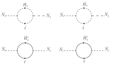
Figure 1: Feynman diagrams contributing to the RHSN self-energies at one-loop.

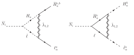
Figure 2: Feynman diagrams contributing to the RHSN decay vertex at one-loop.

The total CP asymmetry in the decays of $\widetilde{N}_{\pm}$ is defined as:

$$\epsilon_{\alpha}=\frac{\displaystyle\sum_{i=\pm,a_{\alpha}}\left[\gamma(\widetilde{N}_{i}\rightarrow a_{\alpha})-\gamma(\widetilde{N}_{i}\rightarrow\bar{a}_{\alpha})\right]}{\displaystyle\sum_{i=\pm,a_{\beta},\beta}\left[\gamma(\widetilde{N}_{i}\rightarrow a_{\beta})+\gamma(\widetilde{N}_{i}\rightarrow\bar{a}_{\beta})\right]},$$ (23)

where $\gamma(\widetilde{N}_{i}\to a_{\alpha})$ is the thermally averaged decay rate for the decay of $\widetilde{N}_{i}$ into final state $a_{\alpha}$ ($a_{\alpha}\equiv s_{\alpha},f_{\alpha}$ with $s_{\alpha}=\tilde{\ell}^{a}_{\alpha}H_{u}^{b}$ and $f_{\alpha}=\ell_{\alpha}^{a}\widetilde{H}_{u}^{c,b}$).

Ignoring thermal effects and taking into account only the mass splitting in the decay width and amplitudes, Eq. (23) becomes

$$\epsilon_{\alpha}(T=0) = \frac{\displaystyle\sum_{i=\pm,a_{\alpha}}\left(|\hat{\mathcal{A}}_{i}^{a_{\alpha}}|^{2}-|\overline{\hat{\mathcal{A}}_{i}^{\bar{a}_{\alpha}}}|^{2}\right)/M_{i}}{\displaystyle\sum_{i=\pm,a_{\beta},\beta}\left(|\hat{\mathcal{A}}_{i}^{a_{\beta}}|^{2}+|\overline{\hat{\mathcal{A}}_{i}^{\bar{a}_{\beta}}}|^{2}\right)/M_{i}},$$ (24)

where $\hat{\mathcal{A}}_{i}^{{a}_{\alpha}}$ is the amplitude for the decay of $\widetilde{N}_{i}$ into $a_{\alpha}$.

To fully account for finite temperature corrections several different effects must be considered:

1. Thermal corrections to (s)leptons and Higgs(inos) propagators,

2. Final state statistical factors,

3. Thermal masses of (s)leptons and Higgs(inos),

4. Thermal corrections to gauge and Yukawa couplings,

5. Particle motion in the thermal bath.

In the two pioneering papers[50, 51] it was shown that the most relevant thermal effects in SL are those of type (B) that arise from final state Bose-enhancement and Fermi-blocking for RHSN decays respectively into scalars and fermions. These effects spoil the cancellation between the decay asymmetries into scalars and fermions, and are large enough to render SL viable. In Ref. Grossman:2003 only effects of type (B) were taken into account. In Ref. DAmbrosio:2003 effects of types (C) and (D) were also included, but it was found that they did not change significantly the overall picture. However, in all these studies, effect (E) was always ignored. Later, the authors of Ref. Giudice:2003jh studied the full-fledged thermal effects (A)-(D), and concluded that all the effects previously neglected did not introduce significant changes. As regards specifically the effects of type (E), Refs. Covi:1997dr,Giudice:2003jh showed that in the case of SM type I leptogenesis the related corrections are at most $\sim 20\%$ with respect to the $T=0$ case, which suggests that they can be neglected also in SL.

Including only the main thermal effects (B), (C) and (D) the total CP asymmetry (23) simplifies to:

$$\epsilon_{\alpha}=\epsilon_{+\alpha}^{s}+\epsilon_{-\alpha}^{s}+\epsilon_{+\alpha}^{f}+\epsilon_{-\alpha}^{f},$$ (25)

where

$$\epsilon^{s}_{\pm\alpha}=\frac{\displaystyle\left(|\hat{\mathcal{A}}_{\pm}^{s_{\alpha}}|^{2}-|\overline{\hat{\mathcal{A}}_{\pm}^{\bar{s}_{\alpha}}}|^{2}\right)c^{s_{\alpha}}_{\pm}/M_{i}}{\displaystyle\sum_{i=\pm,a_{\beta},\beta}\left(|\hat{\mathcal{A}}_{i}^{a_{\beta}}|^{2}+|\overline{\hat{\mathcal{A}}_{i}^{\bar{a}_{\beta}}}|^{2}\right)c^{a_{\beta}}_{i}/M_{i}}\;,$$ (26)

$$\epsilon_{\pm\alpha}^{f}=\frac{\left(|\hat{\mathcal{A}}_{\pm}^{f_{\alpha}}|^{2}-|\overline{\hat{\mathcal{A}}_{\pm}^{\bar{f}_{\alpha}}}|^{2}\right)c^{f_{\alpha}}_{\pm}/M_{i}}{\displaystyle\sum_{i=\pm,a_{\beta},\beta}\left(|\hat{\mathcal{A}}_{i}^{a_{\beta}}|^{2}+|\overline{\hat{\mathcal{A}}_{i}^{\bar{a}_{\beta}}}|^{2}\right)c^{a_{\beta}}_{i}/M_{i}}\;.$$ (27)

In these equations the finite temperature corrections from thermal phase-space, final state Bose-enhancement for decays into scalars and Fermi-blocking for decays into fermions have been factored out in the thermal coefficients $c^{s_{\alpha}}_{\pm},c^{f_{\alpha}}_{\pm}$, so that $\hat{\mathcal{A}}_{i}^{a_{\alpha}}$ and $\overline{\hat{\mathcal{A}}_{i}^{\bar{a}_{\alpha}}}$ are the zero temperature amplitudes. Note that as long as the zero temperature lepton and slepton masses and small neutrino Yukawa couplings are neglected, the thermal coefficients are flavour independent, and if the mass splitting between $\widetilde{N}_{+}$ and $\widetilde{N}_{-}$ is also ignored, they are the same also for $i=\pm$. In the approximation in which $\widetilde{N}_{\pm}$ decay at rest the thermal coefficients are given by:

$$c^{f}_{\pm}\equiv c^{f}(T) = (1-x_{\ell}-x_{\widetilde{H}_{u}})\lambda(1,x_{\ell},x_{\widetilde{H}_{u}})\,\left[1-f_{\ell}^{eq}\right]\left[1-f_{\widetilde{H}_{u}}^{eq}\right],$$ (28)

$$c^{s}_{\pm}\equiv c^{s}(T) = \lambda(1,x_{H_{u}},x_{\tilde{\ell}})\,\left[1+f_{H_{u}}^{eq}\right]\left[1+f_{\widetilde{\ell}}^{eq}\right],$$ (29)

where

$$\lambda(1,x,y)=\sqrt{(1+x-y)^{2}-4x},\qquad x_{a}\equiv\frac{m_{a}(T)^{2}}{M^{2}}\,,$$ (30)

and

$$f^{eq}_{H_{u},\tilde{\ell}}=\frac{1}{\exp[E_{H_{u},\widetilde{\ell}}/T]-1}, f^{eq}_{\widetilde{H}_{u},\ell}=\frac{1}{\exp[E_{\widetilde{H}_{u},\ell}/T]+1},$$ (31)

are the Bose-Einstein and Fermi-Dirac equilibrium distributions, respectively, with

$$E_{\ell,\widetilde{H}_{u}}=\frac{M}{2}(1+x_{\ell,\widetilde{H}_{u}}-x_{\widetilde{H}_{u},\ell}),\qquad E_{H_{u},\widetilde{\ell}}=\frac{M}{2}(1+x_{H_{u},\widetilde{\ell}}-x_{\widetilde{\ell},H_{u}}).$$ (32)

The CP asymmetry is generated at the loop level from the interference between the tree-level and the one-loop diagrams shown in Figs. 1 and 2, that correspond to different sources of CP violation: the first one arises from the self-energy corrections (Fig. 1) while the second arises from vertex corrections (Fig. 2). In the following we describe how the decay asymmetries are computed within two different approaches: the first one relies on field theory, the second one on quantum mechanics.

2.2.1 Field theoretical approach

When $\Gamma\gg\Delta M_{\pm}\equiv M_{+}-M_{-}$, the two RHSN states are not well-separated particles.[51] In this case, the result for the asymmetry depends on how the initial state is prepared. In what follows we assume that the RHSN are in a thermal bath with a thermalization time $\Gamma^{-1}$ shorter than the typical oscillation time $\Delta M_{\pm}^{-1}$. In this case coherence is lost, and it is appropriate to compute the CP asymmetries in terms of the mass eigenstates (14). The relevant decay amplitudes can be obtained following the effective field-theoretical approach described in Refs. Pilaftsis:1997,Pilaftsis:2004,Pilaftsis:2005a,Pilaftsis:2005b,Pilaftsis:2008, which takes into account CP violation due to mixing and decay (as well as their interference) of nearly degenerate states, by using resummed propagators for unstable mass eigenstate particles. The decay amplitude $\hat{\mathcal{A}}_{i}^{a_{\alpha}}$ of the unstable external state $\widetilde{N}_{i}$ into final state $a_{\alpha}$ ($a_{\alpha}\equiv s_{\alpha},f_{\alpha}$ with $s_{\alpha}=\tilde{\ell}^{a}_{\alpha}H_{u}^{b}$ and $f_{\alpha}=\ell_{\alpha}^{a}\widetilde{H}_{u}^{c,b}$) is described by a superposition of amplitudes with stable final states:

$$\hat{\mathcal{A}}_{\pm}^{a_{\alpha}} \!=\! \left(A_{\pm}^{a_{\alpha}}+i{\mathcal{V}_{\pm}^{a_{\alpha}}}^{{\rm abs}}(p^{2})\right)-\left(A_{\mp}^{a_{\alpha}}+i{\mathcal{V}_{\mp}^{a_{\alpha}}}^{{\rm abs}}(p^{2})\right)\times\frac{i\Sigma_{\mp\pm}^{{\rm abs}}}{M_{\pm}^{2}-M_{\mp}^{2}+i\Sigma_{\mp\mp}^{{\rm abs}}},$$ (33)

$$\overline{\hat{\mathcal{A}}_{\pm}^{\bar{a}_{\alpha}}} \!=\! \left({A_{\pm}^{a_{\alpha}}}^{*}\!+i{\mathcal{V}_{\pm}^{a_{\alpha}}}^{{\rm abs}*}(p^{2})\right)-\left({A_{\mp}^{a_{\alpha}}}^{*}\!\!+i{\mathcal{V}_{\mp}^{a_{\alpha}}}^{{\rm abs}*}(p^{2})\right)\!\times\!\frac{i\overline{\Sigma}_{\mp\pm}^{{\rm abs}}}{M_{\pm}^{2}\!-M_{\mp}^{2}\!+i\overline{\Sigma}_{\mp\mp}^{{\rm abs}}}\,.\;\;\;$$ (34)

In these equations $A_{\pm}^{a_{\alpha}}$ are the tree-level amplitudes:

$$\!\!\!A_{+}^{s_{\alpha}} = \frac{Y_{\alpha}}{\sqrt{2}}(A^{*}+M)\epsilon_{ab},\;\;\;\;\;\;\;\;\;\;\ \ \quad A_{-}^{s_{\alpha}}=-i\frac{Y_{\alpha}}{\sqrt{2}}(A^{*}-M)\epsilon_{ab},$$ (35)

$$\!\!\!A_{+}^{f_{k}} = \frac{Y_{\alpha}}{\sqrt{2}}[\bar{u}(p_{\ell})P_{R}v(p_{\widetilde{H}_{u}^{c}})]\epsilon_{ab},\;\;\;\quad A_{-}^{f_{\alpha}}=-i\frac{Y_{\alpha}}{\sqrt{2}}[\bar{u}(p_{\ell})P_{R}v(p_{\widetilde{H}_{u}^{c}})]\epsilon_{ab}.$$ (36)

$\Sigma_{ij}^{{\rm abs}}$ are the absorptive parts of the $\widetilde{N}_{i}\to\widetilde{N}_{j}$ self-energies (see Fig. 1) which can be obtain by directly evaluating the imaginary part of the Feynman integral or by using Cutkosky’s cutting rules:[80]

$$\Sigma_{\mp\mp}^{(1){\rm abs}} = \Gamma\;M\left[\frac{1}{2}+\frac{M_{\mp}^{2}}{2M^{2}}+\frac{|A|^{2}}{2M^{2}}\mp\frac{\mbox{Re}(A)}{M}\right],$$ (37)

$$\Sigma_{\mp\pm}^{(1){\rm abs}} = -\Gamma\;\mbox{Im}(A).$$ (38)

${\mathcal{V}_{\pm}^{a_{\alpha}}}^{{\rm abs}}$ are the absorptive parts of the vertex corrections (see Fig. 2):

$${\mathcal{V}_{+}^{s_{\alpha}}}^{{\rm abs}}\left(p^{2}\right) = \epsilon_{ab}\frac{Y_{\alpha}}{\sqrt{2}}\frac{3m_{2}}{32\pi}(g_{2})^{2}\ln\frac{m_{2}^{2}}{p^{2}+m_{2}^{2}}\;,$$ (39)

$${\mathcal{V}_{-}^{s_{\alpha}}}^{\rm abs}\left(p^{2}\right) = -i\epsilon_{ab}\frac{Y_{\alpha}}{\sqrt{2}}\frac{3m_{2}}{32\pi}(g_{2})^{2}\ln\frac{m_{2}^{2}}{p^{2}+m_{2}^{2}}\;,$$ (40)

$${\mathcal{V}_{+}^{f_{\alpha}}}^{{\rm abs}}\left(p^{2}\right) = \epsilon_{ab}\frac{Y_{\alpha}}{\sqrt{2}}\frac{3m_{2}}{32\pi p^{2}}(A^{*}+M)(g_{2}^{*})^{2}\ln\frac{m_{2}^{2}}{p^{2}+m_{2}^{2}}\times[\bar{u}(p_{\ell})P_{R}v(p_{\widetilde{H}_{u}^{c}})],\quad$$ (41)

$${\mathcal{V}_{-}^{f_{\alpha}}}^{{\rm abs}}\left(p^{2}\right) = -i\epsilon_{ab}\frac{Y_{\alpha}}{\sqrt{2}}\frac{3m_{2}}{32\pi p^{2}}(A^{*}-M)(g_{2}^{*})^{2}\ln\frac{m_{2}^{2}}{p^{2}+m_{2}^{2}}\times[\bar{u}(p_{\ell})P_{R}v(p_{\widetilde{H}_{u}^{c}})],\quad$$ (42)

where only the contribution from $SU(2)_{L}$ gauginos has been included. The contribution from $U(1)_{Y}$ gaugino can be obtained by simply substituting $\alpha_{2}\to\alpha_{Y}\equiv\frac{|g_{Y}|^{2}}{4\pi}$ and $3\to 1$ in Eqs. (39)–(42).

Substituting Eqs. (33) and (34) into Eqs. (26) and (27) and using that $\Sigma_{\mp\mp}^{{\rm abs}}=\overline{\Sigma}_{\mp\mp}^{{\rm abs}}$ and $\Sigma_{\mp\pm}^{{\rm abs}*}=\overline{\Sigma}_{\mp\pm}^{{\rm abs}}$, one gets:

$$|\hat{\mathcal{A}}_{\pm}^{a_{\alpha}}|^{2}-|\overline{\hat{\mathcal{A}}_{\pm}^{\bar{a}_{\alpha}}}|^{2} \simeq -4\left\{-\mbox{Im}\left[{A_{\pm}^{a_{\alpha}}}^{*}A_{\mp}^{a_{\alpha}}\Sigma_{\mp\pm}^{{\rm abs}}\right]\frac{M_{\pm}^{2}-M_{\mp}^{2}}{(M_{\pm}^{2}-M_{\mp}^{2})^{2}+|\Sigma_{\mp\mp}^{{\rm abs}}|^{2}}\right.$$ (43)

$$+\mbox{Im}\left[{A_{\pm}^{a_{\alpha}}}^{*}{\mathcal{V}_{\pm}^{a_{\alpha}}}^{{\rm abs}}(M^{2}_{\pm})\right]$$

$$\left.+\mbox{Im}\left[{\mathcal{V}_{\pm}^{a_{\alpha}}}^{{\rm abs}*}(M^{2}_{\pm})A_{\mp}^{a_{\alpha}}\Sigma_{\mp\pm}^{{\rm abs}}-{A_{\pm}^{a_{\alpha}}}^{*}{\mathcal{V}_{\mp}^{a_{\alpha}}}^{{\rm abs}}(M^{2}_{\pm})\Sigma_{\mp\pm}^{{\rm abs}}\right]\right.$$

$$\left.\times\frac{\Sigma_{\mp\mp}^{{\rm abs}}}{(M_{\pm}^{2}-M_{\mp}^{2})^{2}+|\Sigma_{\mp\mp}^{{\rm abs}}|^{2}}\right\},$$

where the $\simeq$ sign means that terms of order $\delta_{S}^{3}$ and higher are ignored, with $\delta_{S}$ defined in Eq. (21). The three terms inside curly brackets in Eq. (43) correspond respectively to CP violation in $\widetilde{N}$ mixing from the off-diagonal one-loop self-energies that will be denoted below with $S$ (=‘self-energy’), CP violation due to the gaugino-mediated one-loop vertex corrections to the $\widetilde{N}$ decay[81] denoted by $V$ (=‘vertex’), and CP violation in the interference of vertex and self-energies denoted by $I$ (=‘interference’). On the other hand, the amplitudes appearing in the denominators in Eqs. (26) – (27) verify the tree-level relations $|\hat{\mathcal{A}}_{\pm}^{a_{\alpha}}|^{2}+|\overline{\hat{\mathcal{A}}_{\pm}^{\bar{a}_{\alpha}}}|^{2}=2|A_{\pm}^{a_{\alpha}}|^{2}$, with $|A_{\pm}^{s_{\alpha}}|^{2}=Y_{\alpha}^{2}\left[|A|^{2}+M^{2}\pm 2M\mbox{Re}(A)\right]$ and $|A_{\pm}^{f_{\alpha}}|^{2}=Y_{\alpha}^{2}M_{\pm}^{2}$.

Using the explicit forms in Eqs. (35) – (42) one can verify that the the three contributions $S$, $V$ and $I$ to the CP asymmetry from scalar and fermion decays satisfy :

$$\epsilon_{\pm\alpha}^{sS}=\Delta^{s}(T)\epsilon^{S}_{\pm\alpha},\;\;\;\;\;\;\;\;\epsilon_{\pm\alpha}^{fS}=-\Delta^{f}(T)\epsilon^{S}_{\pm\alpha},$$

$$\epsilon_{\pm\alpha}^{sV}=\Delta^{s}(T)\epsilon^{V}_{\pm\alpha},\;\;\;\;\;\;\;\;\epsilon_{\pm\alpha}^{fV}=-\Delta^{f}(T)\epsilon^{V}_{\pm\alpha},$$

$$\epsilon_{\pm\alpha}^{sI}=\Delta^{s}(T)\epsilon^{I}_{\pm\alpha},\;\;\;\;\;\;\;\;\epsilon_{\pm\alpha}^{fI}=-\Delta^{f}(T)\epsilon^{I}_{\pm\alpha},$$ (44)

with

$$\!\!\!\epsilon_{\pm\alpha}^{S} = -P_{\alpha}\frac{A}{M}\sin\left(\phi_{A}\right)\frac{2B\Gamma}{4B^{2}+\Gamma^{2}},$$ (45)

$$\!\!\!\!\!\!\epsilon_{\pm\alpha}^{V} = -\frac{3P_{\alpha}\alpha_{2}}{8}\frac{m_{2}}{M}\ln\frac{m_{2}^{2}}{m_{2}^{2}+M^{2}}\left[\frac{A}{M}\sin\left(\phi_{A}+2\phi_{g}\right)-\frac{B}{M}\sin\left(2\phi_{g}\right)\pm\sin\left(2\phi_{g}\right)\right]\!,\quad\ \$$ (46)

$$\!\!\!\epsilon_{\pm\alpha}^{I} = \frac{3P_{\alpha}\alpha_{2}}{4}\frac{m_{2}}{M}\frac{A}{M}\ln\frac{m_{2}^{2}}{m_{2}^{2}+M^{2}}\sin\left(\phi_{A}\right)\cos\left(2\phi_{g}\right)\frac{\Gamma^{2}}{4B^{2}+\Gamma^{2}},$$ (47)

and

$$\Delta_{s,f}(T)\equiv\frac{c^{s,f}(T)}{c^{s}(T)+c^{f}(T)}.$$ (48)

In the expressions Eqs. (45)-(47) we have introduced $\alpha_{2}=\frac{|g_{2}|^{2}}{4\pi}$, and the physical complex phases $\phi_{A}$ and $\phi_{g}\equiv\phi_{g_{2}}$ have been explicitly written, so that all the parameters $A$ and $Y_{\alpha}$ etc. are understood to be real and positive. We will adopt this convention also in the following, unless explicitly stated in the text. The flavour projectors are defined as

$$P_{\alpha}=\frac{Y_{\alpha}^{2}}{{\displaystyle\sum_{\beta}}Y_{\beta}^{2}},$$ (49)

and satisfy the conditions

$$\sum_{\alpha}P_{\alpha}=1\quad{\rm and}\quad 0\leq P_{\alpha}\leq 1\,.$$ (50)

Summing up the contributions from the decays of $\widetilde{N}_{+}$ and $\widetilde{N}_{-}$ into scalars and fermions, one obtains the three contributions to the total CP asymmetry Eq. (23):[82]

$$\epsilon_{\alpha}^{S}(T) = P_{\alpha}\bar{\epsilon}^{S}\Delta_{BF}(T),$$ (51)

$$\epsilon_{\alpha}^{V}(T) = P_{\alpha}\bar{\epsilon}^{V}\Delta_{BF}(T),$$ (52)

$$\epsilon_{\alpha}^{I}(T) = P_{\alpha}\bar{\epsilon}^{I}\Delta_{BF}(T),$$ (53)

where

$$\bar{\epsilon}^{S} \equiv -\frac{A}{M}\sin\left(\phi_{A}\right)\frac{4B\Gamma}{4B^{2}+\Gamma^{2}},$$ (54)

$$\bar{\epsilon}^{V} \equiv -\frac{3\alpha_{2}}{4}\frac{m_{2}}{M}\ln\frac{m_{2}^{2}}{m_{2}^{2}+M^{2}}\left[\frac{A}{M}\sin\left(\phi_{A}+2\phi_{g}\right)-\frac{B}{M}\sin\left(2\phi_{g}\right)\right],$$ (55)

$$\bar{\epsilon}^{I} \equiv \frac{3\alpha_{2}}{2}\frac{m_{2}}{M}\frac{A}{M}\ln\frac{m_{2}^{2}}{m_{2}^{2}+M^{2}}\sin\left(\phi_{A}\right)\mbox{cos}\left(2\phi_{g}\right)\frac{\Gamma^{2}}{4B^{2}+\Gamma^{2}},$$ (56)

and the thermal factor $\Delta_{BF}(T)$ is given by

$$\Delta_{BF}(T) \equiv \Delta^{s}(T)-\Delta^{f}(T).$$ (57)

Eq. (51) contains the contribution to the asymmetry due to CP violation in RHSN mixing discussed in the original works.[50, 51] Eqs. (52) and (53) give respectively the contribution to the asymmetry from CP violation in decay and in the interference between mixing and decay. These last two contributions have parametric dependence similar to the ones obtained in Ref. Grossman:2004. However, as it is explicitly shown in Eqs. (44), the scalar and fermionic CP asymmetries cancel each other at zero temperature,[82] because as $T\to 0$ both $c^{s}(T),\,c^{f}(T)\to 1$. Consequently up to second order in the soft parameters, all contributions to the SL CP lepton asymmetry require thermal effects in order to be significant. More precisely, $\epsilon_{\alpha}^{V}(T)$ and $\epsilon_{\alpha}^{I}(T)$ vanish exactly in the $T=0$ limit, in agreement with a general proof that will be presented in Section 2.3. As regards $\epsilon_{\alpha}^{S}(T)$, it does not vanish exactly; however, the surviving terms are of order $\mathcal{O}(\delta_{S}^{3})$ and thus completely negligible.

Fig. 3 displays the thermal factors $\Delta_{BF}$ (black solid curve), $\Delta^{s}$ (blue dashed curve) and $\Delta^{f}$ (red dotted curve) as a function of $z\equiv M/T$. For $z\lesssim 0.8$, the decays of RHSN to scalars and fermions are kinematically forbidden. In the small interval $0.8\lesssim z\lesssim 1.2$ the fermionic channel becomes accessible although the scalar channel is still closed; this is because the thermal masses for the fermions are half than the ones for the scalars. For $z\gtrsim 1.2$, the scalar channel opens up as well, however because of thermal effects the cancellation between $\Delta^{s}$ and $\Delta^{f}$ is not very effective, and for relatively small values of $z$ a sizable total asymmetry survives. For $z\ \hbox to0.0pt{\raise 3.0pt\hbox{$>$}\hss}{\lower 3.0pt\hbox{$\sim$}}\ 10$ thermal effects are strongly suppressed and the cancellation becomes almost exact.

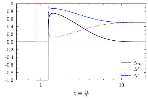
Figure 3: The thermal factors $\Delta_{BF}$ (black solid curve), $\Delta^{s}$ (blue dashed curve) and $\Delta^{f}$ (red dotted curve) as a function of $z\equiv M/T$.

As a final remark, let us note that in this derivation thermal corrections to the loop diagrams responsible for the CP asymmetries have been neglected. That is, the imaginary part of the one-loop graphs has been obtained by directly evaluating the imaginary part of the Feynman integrals or by Cutkosky’s cutting rules at $T=0$.[80]

2.2.2 Quantum mechanical approach

In this section we describe the computation of the CP asymmetry using a quantum mechanical (QM) approach, based on an effective (non Hermitian) Hamiltonian.[50, 51, 81] In this language an analogy can be drawn between the $\widetilde{N}$–$\widetilde{N}^{\dagger}$ system and the system of neutral mesons such as $K^{0}$–$\overline{K}^{0}$, for which the time evolution is determined, in the non-relativistic limit, by the Hamiltonian:

$$H = \left(\begin{array}[]{cc}M&\frac{B}{2}\\ \frac{B}{2}&M\end{array}\right)-\frac{i}{2}\left(\begin{array}[]{cc}\Gamma&\frac{\Gamma A^{*}}{M}\\ \frac{\Gamma A}{M}&\Gamma\end{array}\right),$$ (62)

with $\Gamma$ given in Eq. (22).

In Refs. Grossman:2003,DAmbrosio:2003,Grossman:2004 the QM formalism was applied for weak initial states $\widetilde{N}$ and $\widetilde{N}^{\dagger}$. In practice, the formalism can be applied to study the evolution of initial states that are either weak or mass eigenstates. In order to illustrate the dependence of the results on the choice of initial conditions, we compute the asymmetry for both types of initial states. Let us define the basis:

$$\tilde{N}_{1}=\left(g\tilde{N}+h\tilde{N}^{\dagger}\right),\qquad\tilde{N}_{2}=e^{i\theta}\left(h\tilde{N}-g\tilde{N}^{\dagger}\right).$$ (63)

The mass basis introduced in Eq. (14), corresponds to $(g,h,\theta)=(\frac{1}{\sqrt{2}},\frac{1}{\sqrt{2}},-\frac{\pi}{2})$. Pure $\widetilde{N}$ and $\widetilde{N}^{\dagger}$ initial states correspond instead to $(g,h,\theta)=(1,0,\pi)$.

Including the one-loop contribution from gaugino exchange, the decay amplitudes of $\widetilde{N}_{1}$ and $\widetilde{N}_{2}$ into fermions $f_{\alpha}=\ell_{\alpha}^{a}\widetilde{H}_{u}^{c,b}$ are:

$$A_{1}^{f_{\alpha}} = \left\{Y_{\alpha}h-\frac{3Y_{\alpha}}{2M^{2}}\left(gM+hA^{*}\right)\left(g_{2}^{*}\right)^{2}\frac{m_{2}}{16\pi}I_{f}\right\}[\overline{u}\left(p_{\ell}\right)P_{R}v(p_{\widetilde{H}_{u}^{c}})]\epsilon_{ab},$$

$$\overline{A_{1}^{\bar{f}_{\alpha}}} = \left\{Y_{\alpha}g-\frac{3Y_{\alpha}}{2M^{2}}\left(hM+gA\right)\left(g_{2}\right)^{2}\frac{m_{2}}{16\pi}I_{f}\right\}[\overline{u}(p_{\widetilde{H}_{u}^{c}})P_{L}v\left(p_{\ell}\right)]\epsilon_{ab},$$

$$A_{2}^{f_{\alpha}} = -e^{-i\theta}\left\{Y_{\alpha}g-\frac{3Y_{\alpha}}{2M^{2}}\left(hM-gA^{*}\right)\left(g_{2}^{*}\right)^{2}\frac{m_{2}}{16\pi}I_{f}\right\}[\overline{u}\left(p_{\ell}\right)P_{R}v(p_{\widetilde{H}_{u}^{c}})]\epsilon_{ab},$$

$$\overline{A_{2}^{\bar{f}_{\alpha}}} = e^{-i\theta}\left\{Y_{\alpha}h-\frac{3Y_{\alpha}}{2M^{2}}\left(hA-gM\right)\left(g_{2}\right)^{2}\frac{m_{2}}{16\pi}I_{f}\right\}[\overline{u}(p_{\widetilde{H}_{u}^{c}})P_{L}v\left(p_{\ell}\right)]\epsilon_{ab},$$ (64)

where $\overline{A}$ denotes the decay amplitudes into antifermions. The corresponding decay amplitudes into scalar $s_{\alpha}=\widetilde{\ell}_{\alpha}^{a}H_{u}^{b}$ are:

$$A_{1}^{s_{\alpha}} = \left\{Y_{\alpha}\left(gM+hA^{*}\right)-\frac{3Y_{\alpha}}{2}h\left(g_{2}\right)^{2}\frac{m_{2}}{16\pi}I_{s}\right\}\epsilon_{ab},$$

$$\overline{A_{1}^{\bar{s}_{\alpha}}} = \left\{Y_{\alpha}\left(hM+gA\right)-\frac{3Y_{\alpha}}{2}g\left(g_{2}^{*}\right)^{2}\frac{m_{2}}{16\pi}I_{s}\right\}\epsilon_{ab},$$

$$A_{2}^{s_{\alpha}} = e^{-i\theta}\left\{Y_{\alpha}\left(hM-gA^{*}\right)+\frac{3Y_{\alpha}}{2}g\left(g_{2}\right)^{2}\frac{m_{2}}{16\pi}I_{s}\right\}\epsilon_{ab},$$

$$\overline{A_{2}^{\bar{s}_{\alpha}}} = e^{-i\theta}\left\{Y_{\alpha}\left(hA-gM\right)-\frac{3Y_{\alpha}}{2}h\left(g_{2}^{*}\right)^{2}\frac{m_{2}}{16\pi}I_{s}\right\}\epsilon_{ab}.$$ (65)

In Eqs. (64) and (65):

$$\mbox{Re}(I_{f}) \equiv f_{R}=-\frac{1}{\pi}\left[\frac{1}{2}\left(\ln\frac{m_{2}^{2}}{m_{2}^{2}+M^{2}}\right)^{2}+\mbox{Li}_{2}\left(\frac{m_{2}^{2}}{m_{2}^{2}+M^{2}}\right)-\zeta(2)\right],$$

$$\mbox{Re}(I_{s}) \equiv s_{R}=\frac{1}{\pi}\left[\frac{1}{2}\left(\ln\frac{m_{2}^{2}}{m_{2}^{2}+M^{2}}\right)^{2}+\mbox{Li}_{2}\left(\frac{m_{2}^{2}}{m_{2}^{2}+M^{2}}\right)-\zeta(2)\right.$$

$$+B_{0}\left(M^{2},m_{2},0\right)+B_{0}\left(M^{2},0,m_{2}\right)\Biggr{]},$$

$$\mbox{Im}(I_{f}) \equiv f_{I}=\mbox{Im}(I_{s})\equiv s_{I}=-\ln\frac{m_{2}^{2}}{m_{2}^{2}+M^{2}}.$$ (66)

In terms of $\widetilde{N}_{1}$ and $\widetilde{N}_{2}$ the eigenvectors of the Hamiltonian are:

$$\left|\tilde{N}_{L}\right\rangle = \left(gp+hq\right)\left|\tilde{N}_{1}\right\rangle+e^{-i\theta}\left(hp-gq\right)\left|\tilde{N}_{2}\right\rangle,$$

$$\left|\tilde{N}_{H}\right\rangle = \left(gp-hq\right)\left|\tilde{N}_{1}\right\rangle+e^{-i\theta}\left(hp+gq\right)\left|\tilde{N}_{2}\right\rangle,$$ (67)

where

$$\frac{q}{p} = -1-\frac{\Gamma A}{BM}\sin\left(\phi_{A}\right)-\frac{\Gamma^{2}A^{2}}{M^{2}B^{2}}\cos^{2}\left(\phi_{A}\right)-\frac{i}{2}\frac{\Gamma^{2}A^{2}}{M^{2}B^{2}}\sin\left(2\phi_{A}\right).$$ (68)

At time $t$ the states $\widetilde{N}_{1}$ and $\widetilde{N}_{2}$ evolve into

$$\left|\tilde{N}_{1,2}(t)\right\rangle = \frac{1}{2}\left\{\left[e_{L}(t)+e_{H}(t)\pm C_{0}\left(e_{L}(t)-e_{H}(t)\right)\right]\left|\tilde{N}_{1,2}\right\rangle\right.$$ (69)

$$\left.+e^{\mp i\theta}C_{1,2}\left(e_{L}(t)-e_{H}(t)\right)\left|\tilde{N}_{2,1}\right\rangle\right\}\;,$$

where

$$C_{0}=gh\left(\frac{p}{q}+\frac{q}{p}\right),\;\;\;\;C_{1}=h^{2}\frac{p}{q}-g^{2}\frac{q}{p},\;\;\;\;C_{2}=h^{2}\frac{q}{p}-g^{2}\frac{p}{q},\;\;\;\;$$ (70)

and

$$e_{H,L}(t) \equiv e^{-i(M_{H,L}-\frac{i}{2}\Gamma_{H,L})t}.$$ (71)

The total time integrated CP asymmetry is

$$\epsilon_{\alpha}^{QM}=\frac{\displaystyle\sum_{i=1,2,a_{\alpha}}\Gamma(\widetilde{N}_{i}\rightarrow a_{\alpha})-\Gamma(\widetilde{N}_{i}\rightarrow\bar{a}_{\alpha})}{\displaystyle\sum_{i=1,2,a_{\beta},\beta}\Gamma(\widetilde{N}_{i}\rightarrow a_{\beta})+\Gamma(\widetilde{N}_{i}\rightarrow\bar{a}_{\beta})}\ ,$$ (72)

where the time integrated rates $\Gamma(\widetilde{N}_{i}\rightarrow a_{\alpha})$ can be obtained from Eq. (69):

$$\Gamma(\widetilde{N}_{i}\rightarrow a_{\alpha}) = \frac{1}{4}\frac{c^{a_{\alpha}}}{16\pi M}\biggl{(}\left|A^{a_{\alpha}}_{i}\right|^{2}G_{i+}+\left|A_{j\neq i}^{a_{\alpha}}\right|^{2}G_{j-}$$ (73)

$$+2\left[\mbox{Re}\left({A^{a_{\alpha}}_{i}}^{*}A^{a_{\alpha}}_{j\neq i}\right)G_{ii}^{R}-\mbox{Im}\left({A^{a_{\alpha}}_{i}}^{*}A^{a_{\alpha}}_{j\neq i}\right)G_{ii}^{I}\right]\biggr{)},$$

and the rates $\Gamma(\widetilde{N}_{i}\rightarrow\bar{a}_{\alpha})$ for antiparticles are obtained by replacing $A^{a_{\alpha}}_{i}\rightarrow\overline{A^{\bar{a}_{\alpha}}_{i}}$. In Eq. (73) we have introduced the time integrated projections

$$G_{1(2)+} = 2\left(\frac{1}{1-y^{2}}+\frac{1}{1+x^{2}}\right)+2\left|C_{0}\right|^{2}\left(\frac{1}{1-y^{2}}-\frac{1}{1+x^{2}}\right)$$ (74)

$$\pm 8\left[\mbox{Re}\left(C_{0}\right)\frac{y}{1-y^{2}}-\mbox{Im}\left(C_{0}\right)\frac{x}{1+x^{2}}\right],$$

$$G_{1(2)-} = 2\left|C_{1,2}\right|^{2}\left(\frac{1}{1-y^{2}}-\frac{1}{1+x^{2}}\right),$$ (75)

$$G_{11(22)}^{R} = 2\left\{\mbox{Re}\left[e^{\mp i\theta}C_{1(2)}\right]\frac{y}{1-y^{2}}-\mbox{Im}\left[e^{\mp i\theta}C_{1(2)}\right]\frac{x}{1+x^{2}}\right\}$$ (76)

$$\pm 2\mbox{Re}\left[e^{\mp i\theta}C_{0}^{*}C_{1(2)}\right]\left(\frac{1}{1-y^{2}}-\frac{1}{1+x^{2}}\right),$$

$$G_{11(22)}^{I} = 2\left\{\mbox{Im}\left[e^{\mp i\theta}C_{1(2)}\right]\frac{y}{1-y^{2}}+\mbox{Re}\left[e^{\mp i\theta}C_{1(2)}\right]\frac{x}{1+x^{2}}\right\}$$ (77)

$$\pm 2\mbox{Im}\left[e^{\mp i\theta}C_{0}^{*}C_{1(2)}\right]\left(\frac{1}{1-y^{2}}-\frac{1}{1+x^{2}}\right),$$

written in terms of the mass and width differences:

$$x = \frac{M_{H}-M_{L}}{\Gamma}=\frac{B}{\Gamma}-\frac{1}{2}\frac{\Gamma A^{2}}{BM^{2}}\sin^{2}\left(\phi_{A}\right),$$

$$y = \frac{\Gamma_{H}-\Gamma_{L}}{2\Gamma}=\frac{A}{M}\cos\left(\phi_{A}\right)-\frac{B}{2M}.$$ (78)

Using Eqs. (73)–(77) one can write the numerator in Eq. (72) as

$$\sum_{i}\Gamma(\widetilde{N}_{i}\rightarrow a_{\alpha})-\Gamma(\widetilde{N}_{i}\rightarrow\bar{a}_{\alpha})\equiv\Delta\Gamma^{a_{\alpha},R}+\Delta\Gamma^{a_{\alpha},NR}+\Delta\Gamma^{a_{\alpha},I},$$ (79)

with

$$\Delta\Gamma^{a_{\alpha},R} = \frac{1}{2}\frac{c^{a_{\alpha}}}{16\pi M}\frac{x^{2}+y^{2}}{\left(1-y^{2}\right)\left(1+x^{2}\right)}\Biggl{\{}\left|C_{0}\right|^{2}{\cal F}_{1+}-\frac{\left(\left|C_{1}\right|^{2}-\left|C_{2}\right|^{2}\right)}{2}{\cal F}_{1-}$$ (80)

$$+2\left[\mbox{Re}{\cal F}_{2-}\mbox{Re}\left(e^{-i\theta}C_{0}^{*}C_{1}\right)\right.\left.-\mbox{Re}{\cal F}_{3+}\mbox{Re}\left(e^{i\theta}C_{0}^{*}C_{2}\right)\right]$$

$$-2\left[\mbox{Im}{\cal F}_{2-}\mbox{Im}\left(e^{-i\theta}C_{0}^{*}C_{1}\right)\right.\left.-\mbox{Im}{\cal F}_{3+}\mbox{Im}\left(e^{i\theta}C_{0}^{*}C_{2}\right)\right]\Biggr{\}},$$

$$\Delta\Gamma^{a_{\alpha},NR} = \frac{c^{a_{\alpha}}}{16\pi M}\frac{1}{\left(1-y^{2}\right)}\Biggl{\{}2y\mbox{Re}(C_{0}){\cal F}_{1-}+{\cal F}_{1+}$$ (81)

$$+y\left[\mbox{Re}{\cal F}_{2-}\mbox{Re}\left(e^{-i\theta}C_{1}\right)\right.\left.+\mbox{Re}{\cal F}_{3-}\mbox{Re}\left(e^{i\theta}C_{2}\right)\right]$$

$$-y\left[\mbox{Im}{\cal F}_{2-}\mbox{Im}\left(e^{-i\theta}C_{1}\right)\right.\left.+\mbox{Im}{\cal F}_{3-}\mbox{Im}\left(e^{i\theta}C_{2}\right)\right]\Biggr{\}},$$

$$\Delta\Gamma^{a_{\alpha},I} = \frac{c^{a_{\alpha}}}{16\pi M}\frac{x}{\left(1+x^{2}\right)}\Biggl{\{}-2\mbox{Im}(C_{0}){\cal F}_{1-}$$ (82)

$$-\left[\mbox{Re}{\cal F}_{2-}\mbox{Re}\left(e^{-i\theta}C_{1}\right)\right.\left.+\mbox{Re}{\cal F}_{3-}\mbox{Re}\left(e^{i\theta}C_{2}\right)\right]$$

$$-\left[\mbox{Im}{\cal F}_{2-}\mbox{Im}\left(e^{-i\theta}C_{1}\right)\right.\left.+\mbox{Im}{\cal F}_{3-}\mbox{Im}\left(e^{i\theta}C_{2}\right)\right]\Biggr{\}}\;.$$

where

$${\cal F}_{1\pm} = \left|A^{a_{\alpha}}_{1}\right|^{2}-\left|\overline{A^{\bar{a}_{\alpha}}_{1}}\right|^{2}\pm\left|A^{a_{\alpha}}_{2}\right|^{2}\mp\left|\overline{A^{\bar{a}_{\alpha}}_{2}}\right|^{2}\,,$$ (83)

$${\cal F}_{2\pm} = {A^{a_{\alpha}}_{1}}^{*}A^{a_{\alpha}}_{2}\pm\overline{A^{\bar{a}_{\alpha}}_{1}}^{*}\overline{A^{\bar{a}_{\alpha}}_{2}}\,,$$ (84)

$${\cal F}_{3\pm} = {A^{a_{\alpha}}_{2}}^{*}A^{a_{\alpha}}_{1}\pm\overline{A^{\bar{a}_{\alpha}}_{2}}^{*}\overline{A^{\bar{a}_{\alpha}}_{1}}\,.$$ (85)

In writing the above equations we have classified the contributions as resonant ($R$) if they include an overall factor $\frac{x^{2}+y^{2}}{1+x^{2}}$ and non-resonant ($NR$) if no factor of $\frac{1}{1+x^{2}}$ is present, while the remainder has been labeled as interference ($I$). After substituting the explicit values for the amplitudes and the coefficients, and neglecting all the terms that cancel in both bases, the following relations are obtained:

$$\Delta\Gamma^{f_{\alpha},R}=-c^{f}\Delta\Gamma_{\alpha}^{R}, \;\;\;\;\;\;\Delta\Gamma^{s_{\alpha},R}=c^{s}\Delta\Gamma_{\alpha}^{R},$$

$$\Delta\Gamma^{f_{\alpha},NR}=-c^{f}\Delta\Gamma_{\alpha}^{NR}, \;\;\;\;\;\;\Delta\Gamma^{s_{\alpha},NR}=c^{s}\Delta\Gamma_{\alpha}^{NR},$$

$$\Delta\Gamma^{f_{\alpha},I}=-c^{f}\Delta\Gamma_{\alpha}^{I}, \;\;\;\;\;\;\Delta\Gamma^{s_{\alpha},I}=c^{s}\Delta\Gamma_{\alpha}^{I},$$ (86)

with

$$\Delta\Gamma_{\alpha}^{R} = -\frac{1}{4\pi}Y_{\alpha}^{2}\left[(g^{2}-h^{2})^{2}+(2gh)^{2}\cos(2\theta)\right]A\sin(\phi_{A})$$ (88)

$$\times\frac{1}{x}\frac{x^{2}+y^{2}}{(1-y^{2})(1+x^{2})},$$

$$\Delta\Gamma_{\alpha}^{NR} = \frac{3}{16\pi}Y_{\alpha}^{2}\alpha_{2}\ln\frac{m_{2}^{2}}{m_{2}^{2}+M^{2}}\frac{m_{2}}{M}\frac{1}{1-y^{2}}\left[-A\sin(\phi_{A}+2\phi_{g})\right.$$ (89)

$$\;\;\left.+yM\left(2(2gh)^{2}+(g^{2}-h^{2})^{2}\cos(2\theta)\right)\sin(2\phi_{g})\right],$$

$$\Delta\Gamma_{\alpha}^{I} = \frac{3}{16\pi}Y_{\alpha}^{2}\alpha_{2}\ln\frac{m_{2}^{2}}{m_{2}^{2}+M^{2}}\frac{m_{2}}{M}\frac{1}{1+x^{2}}A$$ (90)

$$\times\sin(\phi_{A})\cos(2\theta)\cos(2\phi_{g}).$$

Eqs. (86) explicitly show that the $T=0$ cancellation of the CP asymmetries occurs also in the QM formalism in both cases of RHSN as initial mass or weak eigenstates. Given that the dependence on the thermal factor $\Delta_{BF}(T)$ Eq. (57) is the same as in the field-theoretical approach and, after normalizing to the total decay width, the same projectors $P_{\alpha}$ Eq. (49) multiply the CP asymmetries, the results can again be recast in terms of flavour and temperature independent quantities $\bar{\epsilon}$ defined as:

$$\epsilon_{\alpha}^{(C)QM(is)}(T)=P_{\alpha}\;\bar{\epsilon}^{(C)QM(is)}\;\Delta_{BF}(T),$$ (91)

where the superscript $(C)=R,\,NR,\,I$ refers to the resonant, non-resonant, and interference contributions, while $(is)=w,m$ refers to the case of weak or mass RHSN initial states. Substituting the values for the coefficients for initial weak RHSN, together with the expressions for $x$ and $y$ in Eqs. (2.2.2) and expanding at order $\delta_{S}^{2}$, one gets

$$\bar{\epsilon}^{R,QM,w} = -\frac{A}{M}\sin\left(\phi_{A}\right)\frac{B\Gamma}{B^{2}+\Gamma^{2}},$$ (92)

$$\bar{\epsilon}^{NR,QM,w} = -\frac{3\alpha_{2}}{4}\frac{m_{2}}{M}\ln\frac{m_{2}^{2}}{m_{2}^{2}+M^{2}}\Big{[}\frac{A}{M}\sin(\phi_{A})\cos(2\phi_{g})+\frac{B}{2M}\sin\left(2\phi_{g}\right)\Big{]},\quad$$ (93)

$$\bar{\epsilon}^{I,QM,w} = \frac{3\alpha_{2}}{4}\frac{m_{2}}{M}\frac{A}{M}\ln\frac{m_{2}^{2}}{m_{2}^{2}+M^{2}}\sin\left(\phi_{A}\right)\mbox{cos}\left(2\phi_{g}\right)\frac{\Gamma^{2}}{B^{2}+\Gamma^{2}}\;.\quad$$ (94)

Correspondingly, for initial $\widetilde{N}_{\pm}$ states one gets:

$$\bar{\epsilon}^{R,QM,m} = \frac{A}{M}\sin\left(\phi_{A}\right)\frac{B\Gamma}{B^{2}+\Gamma^{2}},$$ (95)

$$\bar{\epsilon}^{NR,QM,m} = -\frac{3\alpha_{2}}{4}\frac{m_{2}}{M}\ln\frac{m_{2}^{2}}{m_{2}^{2}+M^{2}}\Big{[}\frac{A}{M}\sin(\phi_{A})\cos(2\phi_{g})+\frac{B}{2M}\sin\left(2\phi_{g}\right)\Big{]},\quad$$ (96)

$$\bar{\epsilon}^{I,QM,m} = -\frac{3\alpha_{2}}{4}\frac{m_{2}}{M}\frac{A}{M}\ln\frac{m_{2}^{2}}{m_{2}^{2}+M^{2}}\sin\left(\phi_{A}\right)\mbox{cos}\left(2\phi_{g}\right)\frac{\Gamma^{2}}{B^{2}+\Gamma^{2}}\;.$$ (97)

Comparing Eqs. (95)–(97) with Eqs. (92)–(94) and Eqs. (54)–(56) one sees that the parametric dependence is very similar, although there are some differences in the numerical coefficients. In particular in either the weak or mass basis $\bar{\epsilon}^{R,QM}$, $\bar{\epsilon}^{I,QM}$ and the $B$-dependent (second term) in $\bar{\epsilon}^{NR,QM}$ coincide with $\bar{\epsilon}^{S}$, $\bar{\epsilon}^{I}$ and the B-dependent term in $\bar{\epsilon}^{V}$ derived in the previous section, modulo the redefinition $A\rightarrow 2A$, $B\rightarrow 2B$ and $\sin(\phi_{A})\rightarrow\pm\sin(\phi_{A})$. There are however, some differences in the phase combination which appears in the $B$ independent term in the asymmetries $\bar{\epsilon}_{\alpha}^{NR,QM}$ and $\bar{\epsilon}_{\alpha}^{V}$ as seen in Eqs. (52), (93) and (96). In other words, the choice of initial state only leads to minor differences. But the crucial role of thermal effects to avoid exact cancellations and to allow for a non-vanishing CP asymmetry is the same in both the QM and field-theoretical approaches, and is independent of the particular basis chosen for the initial RHSN states.

2.3 The vanishing of the CP asymmetry in decays at $T=0$

As we have seen in the previous two sections, the original claim that the sources of direct CP violation from vertex corrections involving the gauginos do not require thermal effects to produce a sizable lepton asymmetry in the plasma[81] is incorrect, and after including vertex corrections the CP asymmetries for decays into scalars and into fermions still cancel in the $T=0$ limit. This issue is of some interest, because if thermal corrections are necessary for SL to work, then non-thermal scenarios, like the ones in which RHSN are produced by inflaton decays and the thermal bath remains at a temperature $T\ll M$ during the following leptogenesis epoch, would be completely excluded. In the following, we present a simple but general argument proving that at $T=0$ the direct leptonic CP violation in RHSN decays vanishes at one loop, due to an exact cancellation between the scalar and fermion contributions.

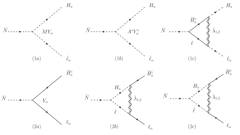
Figure 4: Soft leptogenesis diagrams for RHSN decays into scalars $(1a)$, $(1b)$, $(1c)$ and into fermions $(2a)$, $(2b)$, $(2c)$.

Let us take for simplicity $\Phi=0$ in Eq. (14) (this amounts to assign the phases $\phi_{A}$ and $\phi_{g}$ in Eqs. (17) and (18) respectively to $A$ and $m_{2}$). Since the lepton flavour $\alpha$ will not play a role in this proof, we will suppress in this section the corresponding label. Let us introduce for the various amplitudes the shorthand notation $A^{\pm}_{\ell}\equiv A(\widetilde{N}_{\pm}\to\ell\widetilde{H}_{u}^{c})$, $A^{\widetilde{N}\,(\widetilde{N}^{*})}_{\ell}\equiv A\left(\widetilde{N}\,(\widetilde{N}^{*})\to\ell\widetilde{H}_{u}^{c}\right)$ with similar expressions for the other final states. From Eq. (14) we can write

$$2\,\left|A^{\pm}_{\ell}\right|^{2} = \left|A^{\widetilde{N}}_{\ell}\right|^{2}+\left|A^{\widetilde{N}^{*}}_{\ell}\right|^{2}\pm 2\,\mathrm{Re}\left(A^{\widetilde{N}}_{\ell}\cdot A^{\widetilde{N}}_{\bar{\ell}}\right)\,,$$ (98)

$$2\,\left|A^{\pm}_{\bar{\ell}}\right|^{2} = \left|A^{\widetilde{N}}_{\bar{\ell}}\right|^{2}+\left|A^{\widetilde{N}^{*}}_{\bar{\ell}}\right|^{2}\pm 2\,\mathrm{Re}\left(A^{\widetilde{N}}_{\bar{\ell}}\cdot A^{\widetilde{N}}_{\ell}\right)\,,$$ (99)

where the complex conjugate amplitudes in the last terms of both these equations have been rewritten as follows: $(A^{\widetilde{N}^{*}}_{\ell})^{*}=A_{\widetilde{N}^{*}}^{\ell}=A^{\widetilde{N}}_{\bar{\ell}}$ and $(A^{\widetilde{N}^{*}}_{\bar{\ell}})^{*}=A_{\widetilde{N}^{*}}^{\bar{\ell}}=A^{\widetilde{N}}_{\ell}$ by using CPT invariance in the second step. The direct CP asymmetry for $\widetilde{N}_{\pm}$ decays into fermions is given by the difference between Eqs. (98) and (99):

$$2\,\left(\left|A^{\pm}_{\ell}\right|^{2}-\left|A^{\pm}_{\bar{\ell}}\right|^{2}\right)=\left(\left|A^{\widetilde{N}^{*}}_{\ell}\right|^{2}-\left|A^{\widetilde{N}^{*}}_{\bar{\ell}}\right|^{2}\right)+\left(\left|A^{\widetilde{N}}_{\ell}\right|^{2}-\left|A^{\widetilde{N}}_{\bar{\ell}}\right|^{2}\right)\,.$$ (100)

With the replacements $\ell\to\tilde{\ell}$ and $\bar{\ell}\to\tilde{\ell}^{*}$, a completely equivalent expression holds also for the decays into scalars.

The tree-level and one-loop diagrams for the various decay amplitudes into scalars and fermions are given in Fig. 4. We note at this point that $A^{\widetilde{N}}_{\widetilde{\ell}}$ has no one-loop amplitude to interfere with (see diagram $(1\,a)$) and thus, up to one-loop, the full amplitude coincides with the tree-level result, and is CP conserving. $A^{\widetilde{N}}_{\ell}$ is a pure one-loop amplitude (see diagram $(2\,c)$) and therefore is also CP conserving. It follows that:

$$\left|A^{\widetilde{N}}_{\widetilde{\ell}}\right|^{2}=\left|A^{\widetilde{N}^{*}}_{\widetilde{\ell}^{*}}\right|^{2}\,,\qquad{\rm and}\qquad\left|A^{\widetilde{N}}_{\ell}\right|^{2}=\left|A^{\widetilde{N}^{*}}_{\bar{\ell}}\right|^{2}\,.$$ (101)

We can thus change simultaneously the signs of $\left|A^{\widetilde{N}}_{\ell}\right|^{2}$ and $\left|A^{\widetilde{N}^{*}}_{\bar{\ell}}\right|^{2}$ in eq. (100) without affecting the equality, and the same we can do in the analogous equation for the scalars. This gives:

$$2\,\left(\left|A^{\pm}_{\ell}\right|^{2}-\left|A^{\pm}_{\bar{\ell}}\right|^{2}\right) = \left(\left|A^{\widetilde{N}^{*}}_{\ell}\right|^{2}+\left|A^{\widetilde{N}^{*}}_{\bar{\ell}}\right|^{2}\right)-\left(\left|A^{\widetilde{N}}_{\ell}\right|^{2}+\left|A^{\widetilde{N}}_{\bar{\ell}}\right|^{2}\right)\,,$$ (102)

$$2\,\left(\left|A^{\pm}_{\tilde{\ell}}\right|^{2}-\left|A^{\pm}_{\tilde{\ell}^{*}}\right|^{2}\right) = \left(\left|A^{\widetilde{N}^{*}}_{\tilde{\ell}}\right|^{2}+\left|A^{\widetilde{N}^{*}}_{\tilde{\ell}^{*}}\right|^{2}\right)-\left(\left|A^{\widetilde{N}}_{\tilde{\ell}}\right|^{2}+\left|A^{\widetilde{N}}_{\tilde{\ell}^{*}}\right|^{2}\right)\,.$$ (103)

Using CPT invariance

$$\left|A^{\widetilde{N}^{*}}_{\ell}\right|^{2}+\left|A^{\widetilde{N}^{*}}_{\bar{\ell}}\right|^{2} = \left|A_{\widetilde{N}}^{\bar{\ell}}\right|^{2}+\left|A_{\widetilde{N}}^{\ell}\right|^{2},$$ (104)

$$\left|A^{\widetilde{N}^{*}}_{\tilde{\ell}}\right|^{2}+\left|A^{\widetilde{N}^{*}}_{\tilde{\ell}^{*}}\right|^{2} = \left|A_{\widetilde{N}}^{\tilde{\ell}^{*}}\right|^{2}+\left|A_{\widetilde{N}}^{\tilde{\ell}}\right|^{2},$$ (105)

and unitarity

$$\left|A_{\widetilde{N}}^{\bar{\ell}}\right|^{2}+\left|A_{\widetilde{N}}^{\ell}\right|^{2}+\left|A_{\widetilde{N}}^{\tilde{\ell}^{*}}\right|^{2}+\left|A_{\widetilde{N}}^{\tilde{\ell}}\right|^{2} = \left|A^{\widetilde{N}}_{\bar{\ell}}\right|^{2}+\left|A^{\widetilde{N}}_{\ell}\right|^{2}+\left|A^{\widetilde{N}}_{\tilde{\ell}^{*}}\right|^{2}+\left|A^{\widetilde{N}}_{\tilde{\ell}}\right|^{2}\!,$$ (106)

we can readily see that the sum of zero temperature fermionic CP asymmetry Eq. (102) and scalar CP asymmetry Eq. (103) vanishes. We have thus proved that for $\widetilde{N}_{+}$ and $\widetilde{N}_{-}$ independently, at one loop there is an exact cancellation between the scalar and fermion final state contributions, and thus at $T=0$ the direct decay CP asymmetries vanish.

3 One-flavour Approximation and Superequilibration Regime

3.1 Effective theories in the early Universe

In the expanding early Universe, at each temperature $T$ is associated a characteristic time scale given by the Universe age $t_{U}(T)\sim H^{-1}(T)$ ($H(T)$ being the Hubble parameter at $T$). Particle reactions must be treated in a different way depending if their characteristic time scale $\tau$ (given by inverse of their their thermally averaged rates) is:

• Much shorter than the age of the Universe: $\tau\ll t_{U}(T)$;

• Much larger than the age of the Universe: $\tau\gg t_{U}(T)$;

• Comparable with the Universe age: $\tau\sim t_{U}(T)$.

The first type of reactions (i) occur very frequently during one expansion time and their effects can be simply ‘resummed’ by imposing on the thermodynamic system the chemical equilibrium condition appropriate for each specific reaction, that is $\sum_{I}\mu_{I}=\sum_{F}\mu_{F}$, where $\mu_{I}$ denotes the chemical potential of an initial state particle, and $\mu_{F}$ that of a final state particle. The numerical values of the parameters that are responsible for these reactions only determine the precise temperature $T$ when chemical equilibrium is attained and the resummation of all effects into chemical equilibrium conditions holds but, apart from this, have no other relevance, and do not appear explicitly in the effective formulation of the problem.

Reactions of the second type (ii) cannot have any effect on the system, since they basically do not occur. Then all physical processes are blind to the corresponding parameters, that can be set to zero in the effective Lagrangian. By doing this, it is then easy to read out if new global symmetries appear and, if no anomalies are involved, these symmetries correspond to exactly conserved quantities. The corresponding conservation laws must be respected by the equations describing the dynamics of the system.

Reactions of the third type (iii) in general violate some symmetries, and thus spoil the corresponding conservation conditions, but are not fast enough to enforce chemical equilibrium conditions. Only reactions of this type appear explicitly in the formulation of the problem (they generally enter into a set of Boltzmann equations for the evolution of the system) and only the corresponding parameters represent fundamental quantities in the specific effective theory.

Several examples of the importance of using the appropriate early Universe effective theory can be found in leptogenesis studies. Leptogenesis was first formulated in the so-called ‘one flavour approximation’ in which a single $SU(2)_{L}$ lepton doublet of an unspecified flavour is assumed to couple to the lightest singlet seesaw neutrino, and it is thus responsible for the generation of the lepton asymmetry. Indeed, until the works in Refs. Abada:2006a,Nardi:2006b, most leptogenesis studies were carried out within this framework. Nowadays, it is well understood that the ‘one flavour approximation’ gives a rather rough and often unreliable description of leptogenesis dynamics in the regime when the flavours of the leptons are identified by in-equilibrium charged leptons Yukawa reactions. This is because such an ‘approximation’ has no control over the effects that are neglected, and thus the related uncertainty cannot be estimated. On the other hand, if leptogenesis occurs above $T\sim 10^{12}\,$GeV, when all the charged leptons Yukawa reactions have characteristic time scales much larger than $t_{U}$, the ‘one flavour approximation’ is not at all an approximation. Rather, it is the correct high temperature effective theory that must be used to compute the baryon asymmetry. The corresponding effective Lagrangian is obtained by setting to zero, in the first place, all the charged lepton Yukawa couplings, so that the only remaining flavour structure is determined by the Yukawa couplings of the heavy Majorana neutrinos.

In supersymmetric leptogenesis instead, the effective theory that was generally used was in fact only appropriate for temperatures much lower than the typical temperatures $T\gg 10^{8}\,$GeV in which leptogenesis can be successful, and only quite recently it was clarified that in the relevant temperature range a completely different effective theory holds instead.[71] More specifically, it was always assumed that lepton-slepton reactions like e.g. $\ell\ell\leftrightarrow\tilde{\ell}\tilde{\ell}$ that are induced by soft SUSY-breaking gaugino masses are in thermal equilibrium, and this implies equilibration between the leptons and sleptons density asymmetries (superequilibration). Superequilibration (SE) instead, only occurs below $T\sim 10^{7}\,$GeV, and thus supersymmetric leptogenesis always proceeds in the non-superequilibration (NSE) regime.

As regards SL, it always occurs in a temperature regime in which the charged lepton Yukawa couplings cannot be set to zero, and thus flavour effects must be taken into account, while, since SL can be successful from $T\sim 10^{8}\,$GeV downwards, the two possibilities that it will occur in the SE or in the NSE regimes remain open.

Here, as it was done in the original formulation,[50, 51] we first describe SL taking into account only reactions of type (iii). That is, we will neglect all considerations about flavour effects, that are related to reactions of type (i), as well as NSE effects, that are related to reactions of type (ii). These two issues are addressed respectively in Section 5 and in Section 6.

3.2 Boltzmann equations in the unflavoured approximation

In order to quantify the parameter ranges in which SL is successful one needs to solve the relevant set of Boltzmann equations (BE). All technical details about the BE for SL are given in A.

To eliminate the dependence on the expansion of the Universe it is customary to recast the BE in terms of the variables $Y_{X}=n_{X}/s$, that is in terms of particle number densities $n_{X}$ normalized to the entropy density $s=\frac{2\pi^{2}}{45}g_{*}T^{3}$ where $g_{*}$ is the total number of relativistic degrees of freedom. To account for the sources of violation of lepton number one then needs to follow the evolution of $Y_{\widetilde{N}_{i}}$ and, since RHN decays are also $\Delta L=1$ processes, the evolution of $Y_{N}$ must also be considered.

To simplify the understanding of how a sizable density asymmetry is dynamically generated it is convenient to adopt a certain number of approximations.

The first approximation is to neglect lepton flavours, and work in the so-called ‘one flavour approximation’. The relevant quantities one wants to estimate in this case are the fermionic $Y_{\Delta\ell}$ and scalar $Y_{\Delta\widetilde{\ell}}$ lepton asymmetries generated in the leptonic states coupled to the RHSN (that in general correspond to a superposition of the different lepton flavours). They are defined respectively as $Y_{\Delta\ell}=\left(Y_{\ell}-Y_{\bar{\ell}}\right)/g_{\ell}$ and $Y_{\Delta\widetilde{\ell}}=\left(Y_{\widetilde{\ell}}-Y_{\widetilde{\ell}^{*}}\right)/g_{\widetilde{\ell}}$, that is, we define the density asymmetries for single $SU(2)_{L}$ degree of freedom, with $g_{\ell}=g_{\widetilde{\ell}}=2$.

The second approximation is to neglect all “spectator effects”.[83, 84] Of course, besides the lepton density asymmetries, many other asymmetries related to the finite chemical potentials of the Higgs, higgsinos, quarks and squarks, $SU(2)_{L}$ singlet leptons and sleptons, are also present in the plasma, and affect indirectly the outcome of SL through the so-called spectator effects.[83, 84] In this section all effects of this type will be neglected, which amounts to assume that all particles except the heavy (s)neutrinos and the $SU(2)_{L}$ doublet (s)leptons follow either Bose-Einstein or Fermi-Dirac distribution with vanishing chemical potential $f=(e^{E/T}\mp 1)^{-1}$.

A third simplification arises from the fact that at relatively low temperatures ($T\ \hbox to0.0pt{\raise 3.0pt\hbox{$<$}\hss}{\lower 3.0pt\hbox{$\sim$}}\ 10^{7}\,{\rm GeV}$) reactions that transform leptons into sleptons and vice versa are much faster than the Universe expansion rate. Consequently, the chemical potentials of lepton and slepton equilibrate $\mu_{\ell}=\mu_{\widetilde{\ell}}$ or equivalently $\frac{Y_{\Delta\ell}}{Y_{\ell}^{eq}}=\frac{{Y}_{\Delta\widetilde{\ell}}}{Y_{\widetilde{\ell}}^{eq}}$, a condition known as SE. In the NSE regime $T\ \hbox to0.0pt{\raise 3.0pt\hbox{$>$}\hss}{\lower 3.0pt\hbox{$\sim$}}\ 10^{7}\,{\rm GeV}$ interesting new effects arise that, however, introduce highly non-trivial modifications in the description of SL. For this reason in this section SE is assumed even when the relevant temperature regimes fall above $T\sim 10^{7}\,{\rm GeV}$.

Neglecting SUSY-breaking effects in the RHSN masses and in the vertices, all the amplitudes for $N_{+}$ and $N_{-}$ decays are equal, as well as their corresponding equilibrium number densities, $n_{\widetilde{N}_{+}}^{eq}=n_{\widetilde{N}_{-}}^{eq}\equiv n_{\widetilde{N}}^{eq}$. Thus, in this approximation, a unique BE for $Y_{\widetilde{N}_{\rm tot}}\equiv Y_{\widetilde{N}_{+}}+Y_{\widetilde{N}_{-}}$ suffices to account for the RHSN densities that, together with the BE for $Y_{N}$, give two equations for the out-of-equilibrium heavy neutral states. Using the SE condition $2Y_{\ell}=Y_{\widetilde{\ell}}$ one can combine the BE for the unflavoured asymmetries $Y_{\Delta\ell}$ and $Y_{\Delta\widetilde{\ell}}$ into a single equation by defining a global density asymmetry in the $SU(2)_{L}$ lepton doublets

$$Y_{\Delta\ell_{\rm tot}}\equiv 2\left(Y_{\Delta\ell}+Y_{\Delta\widetilde{\ell}}\right),$$ (107)

where the factor of 2 comes from summing over the $SU(2)_{L}$ degrees of freedom. We can also define a total CP asymmetry

$$\epsilon(T)=\epsilon^{s}(T)+\epsilon^{f}(T)\equiv\bar{\epsilon}\cdot\Delta_{BF}(T),$$ (108)

where

$$\epsilon^{s,f}(T)=\pm\sum_{q=S,V,I}\bar{\epsilon}^{q}\Delta^{s,f}(T),\qquad\qquad\bar{\epsilon}\equiv\sum_{q=S,V,I}\bar{\epsilon}^{q},$$ (109)

and the thermal factor $\Delta_{BF}(T)$ is given in Eq. (57). Given that in the one flavour approximation all lepton flavours are treated on an equal footing, it is left understood that in the previous equations the various components of the CP asymmetry have been simply summed over lepton flavour $\bar{\epsilon}^{q}=\sum_{\alpha}\bar{\epsilon}_{\alpha}^{q}$. The relevant parameters that appear in the CP asymmetries then are $A$, $m_{2}$, $B$, $M$ and the two CP-violating phases $\phi_{A}$ and $\phi_{g}$. The BE for the unflavoured case read:

$$\dot{Y}_{N}\! = -\left(\frac{Y_{N}}{Y_{N}^{eq}}-1\right)\left(\gamma_{N}+4\gamma_{t}^{(0)}+4\gamma_{t}^{(1)}+4\gamma_{t}^{(2)}+2\gamma_{t}^{(3)}+4\gamma_{t}^{(4)}\right),$$ (110)

$$\dot{Y}_{\widetilde{N}_{\rm tot}}\!\! = \!-\!\left(\!\frac{Y_{\widetilde{N}_{\rm tot}}}{Y_{\widetilde{N}}^{eq}}-2\!\right)\!\!\left[\frac{\gamma_{\widetilde{N}}}{2}\!+\gamma_{\widetilde{N}}^{(3)}+3\gamma_{22}+2\!\left(\!\gamma_{t}^{(5)}\!+\gamma_{t}^{(6)}+\gamma_{t}^{(7)}+\gamma_{t}^{(9)}\right)\!+\!\gamma_{t}^{(8)}\!\right]\!\!,\quad\ \$$ (111)

$$\dot{Y}_{\Delta\ell_{\rm tot}} = \,\epsilon(T)\,\left(\frac{Y_{\widetilde{N}_{\rm tot}}}{Y_{\widetilde{N}}^{eq}}-2\right)\frac{\gamma_{\widetilde{N}}}{2}-W\,\frac{Y_{\Delta\ell_{\rm tot}}}{Y_{\ell_{\rm tot}}^{eq}},$$ (112)

where the time derivative is defined as $\dot{Y}_{X}\equiv sHz\frac{dY_{X}}{dz}$ with $z\equiv M/T$, $Y_{\widetilde{N}}^{eq}=n_{\widetilde{N}}^{eq}/s$, and $Y_{\ell_{\rm tot}}^{eq}\equiv\frac{45}{4\pi^{2}g_{*}}$. The washout term $W$ in the equation for ${Y}_{\Delta L_{\rm tot}}$ reads:

$$W = \frac{1}{2}\left(\gamma_{\widetilde{N}}+\gamma_{N}\right)+\gamma_{\widetilde{N}}^{(3)}+\frac{Y_{\widetilde{N}_{\rm tot}}}{Y_{\widetilde{N}}^{eq}}\left(\gamma_{t}^{(5)}+\frac{1}{2}\gamma_{t}^{(8)}\right)+\frac{Y_{N}}{Y_{N}^{eq}}\left(2\gamma_{t}^{(0)}+\gamma_{t}^{(3)}\right)$$ (113)

$$+ 2\left(\gamma_{t}^{(1)}+\gamma_{t}^{(2)}+\gamma_{t}^{(4)}+\gamma_{t}^{(6)}+\gamma_{t}^{(7)}+\gamma_{t}^{(9)}\right)+\left(2+\frac{1}{2}\frac{Y_{\widetilde{N}_{\rm tot}}}{Y_{\widetilde{N}}^{eq}}\right)\gamma_{22}\,.$$

Assuming Maxwell-Boltzmann equilibrium distribution, the RHSN and RHN equilibrium abundances can be written as:

$$Y_{\widetilde{N}}^{eq}=\frac{45}{4\pi^{4}g_{*}}z^{2}\mathcal{K}_{2}(z),\;\;\;\;\;\;Y_{N}^{eq}=\frac{45}{2\pi^{4}g_{*}}z^{2}\mathcal{K}_{2}(z).$$ (114)

(See Ref. Garayoa:2009 for a discussion of the validity of the use of integrated BE.)

The derivation of the factorization of the relevant CP asymmetries including the thermal effects is somewhat lengthy but straightforward (see A.2). The different $\gamma$’s are the thermally averaged reaction densities for the different processes (they are defined in A.2.1). In all cases a sum over the CP conjugate final states and lepton flavours is left implicit.

Eqs. (110)–(112) include the $\widetilde{N}_{\pm}$ and $N$ decay and inverse decay processes as well as all the $\Delta L=1$ scattering processes induced by the top-quark Yukawa coupling. $\Delta L=2$ processes involving the on-shell exchange of $N$ or $\widetilde{N}_{\pm}$ are already accounted for by the decay and inverse decay processes. The $\Delta L=2$ off-shell scatterings involving the pole-subtracted $s$-channel and the $u$- and $t$-channels, as well as the the $L$-conserving processes from $N$ and $\widetilde{N}$ pair creation and annihilation, have not been included. The reaction rates for these processes are quartic in the neutrino Yukawa couplings and therefore can be safely neglected as long as these couplings are much smaller than one, as it is the case for the relevant mass range $M\lesssim 10^{9}\,{\rm GeV}$ required for successful SL (see next section). The non-resonant $\Delta L=2$ processes only become important (strongly suppressing the final asymmetry) when the neutrino Yukawa couplings become of order of one which implies $M\gtrsim 10^{14}\,{\rm GeV}$ (see e.g. Ref. Giudice:2003jh). Note that in Eqs. (110)–(112) only the CP asymmetry in the $\widetilde{N}_{\pm}$ two body decays has been included, while CP violating effects in three body decays and in scatterings[76, 78, 65, 86, 87] have been left out. Strictly speaking, when the effects of washout from scatterings are included, for consistency one should include also the corresponding CP asymmetries. However, in the case of standard leptogenesis it has been found that CP asymmetries in scatterings are important (and dominant) only at high temperatures $z\lesssim 0.5$.[86] Hence they are only relevant in the weak washout regime, and in the case of zero initial RHN abundance.[65, 86] In this case, the inclusion of the scattering CP asymmetries suppresses the final lepton asymmetry because it results in a balance between the two opposite sign lepton asymmetries respectively generated during the RHN production phase and when the RHN eventually decay away, giving rise to a strong cancellation which, in the limit of vanishing washout, is actually exact.[65] In SL, however, the inclusion of the CP asymmetries in scatterings is not straightforward, because scattering thermal factors constitute a new set of non trivial quantities. Nevertheless, it is reasonable to expect that at least for the strong washout regime the effects of scattering CP asymmetries are negligible also in SL. Having said that, a careful quantitative study in this direction is still lacking.

3.3 Leptogenesis efficiency

The effectiveness of leptogenesis for producing a final lepton asymmetry $Y_{\Delta\ell_{\rm tot}}^{\infty}\equiv Y_{\Delta\ell_{\rm tot}}(z\to\infty)$ (or $Y_{\Delta_{B-L}}^{\infty}$ if $L$ violation from sphalerons is accounted for) could be conveniently parametrized in terms of the fractional amount of the maximum available asymmetry that is eventually converted into $Y_{\Delta\ell_{\rm tot}}^{\infty}$. However, such a parametrization can be consistently introduced only for standard thermal leptogenesis when it occurs at temperatures above the onset of flavour effects, and this is because only in this case the maximum available asymmetry can be reliably estimated. In this case $Y_{N}^{eq0}\equiv Y_{\widetilde{N}}^{eq}(z\to 0)$ corresponds to the maximum possible density of decaying RHN, and an amount of $L$-asymmetry equals to $\epsilon$ is produced in each decay. Then the maximum available asymmetry is $\epsilon\cdot Y_{N}^{eq0}$, and one can write

$$Y_{\Delta\ell_{\rm tot}}^{\infty}=\eta\cdot\epsilon\,Y_{N}^{eq0}\,,$$ (115)

where $\eta$ is a non-negative parameter satisfying $0\leq\eta\leq 1$ that represents the leptogenesis efficiency.

However, in other scenarios different from unflavoured thermal leptogenesis it is more difficult to determine the maximum amount of available asymmetry. For example, if the RHN are produced non thermally,[60] it can easily happen that $Y_{N}^{0}$ is much larger than $Y_{N}^{eq0}$, and in this case, if $Y_{\Delta\ell_{\rm tot}}^{\infty}$ is still expressed in units of $\epsilon\,Y_{N}^{eq0}$, values of $\eta>1$ will result. Needless to say, this does not mean that the efficiency of the leptogenesis dynamics is higher than 100%, but it simply follows from underestimating the maximum amount of available asymmetry.

In the presence of flavour effects, the available amount of CP violation is no more described by the total CP asymmetry summed over lepton flavours $\epsilon=\sum_{\alpha}\epsilon_{\alpha}$ ($\alpha=e,\mu,\tau$) but rather by the three flavoured CP asymmetries $\epsilon_{\alpha}$, and it can easily occur that the absolute value of some (or even of all) flavoured CP asymmetries are larger than the absolute value of the total CP asymmetry, with some $\epsilon_{\alpha}$ having a sign opposite to the one of $\epsilon$.[84] Clearly, also in this case $\epsilon\cdot Y_{N}^{eq0}$ does not account for the maximum available asymmetry, and since particular flavour configurations can produce $Y_{\Delta\ell_{\rm tot}}^{\infty}$ with a sign opposite to the one of the total CP asymmetry $\epsilon$, using Eq. (115) could even result in negative values of the ‘efficiency’ $\eta$.

In SL, estimating the maximum amount of available asymmetry is basically an impossible task. This is because, besides the effects of lepton flavours (that is mandatory to include in reliable SL numerical studies, see Section 5) the CP asymmetries for RHSN decays into scalars and fermions $\epsilon^{s,f}(T)$ depend on the temperature and, as it is depicted in Fig. 3, the total CP asymmetry obtained from their sum Eq. (108) can have different signs, depending on the temperature interval considered. Nevertheless, it became customary, and it is often convenient, to express the effectiveness of SL in generating a lepton asymmetry in terms of the fractional amount $\eta$ of a large reference asymmetry $2\,\bar{\epsilon}\,Y_{\widetilde{N}}^{eq0}$, that is:

$$\eta=\left|\frac{Y_{\Delta\ell_{\rm tot}}^{\infty}}{2\,\bar{\epsilon}\,Y_{\widetilde{N}}^{eq0}}\right|\,,$$ (116)

with a similar definition if $Y_{\Delta_{B-L}}^{\infty}$ is considered instead. In the denominator of the r.h.s. of Eq. (116) the factor 2 has been included because there are two RHSN states, while $Y_{\widetilde{N}}^{eq0}=45\,/(2\pi^{4}g_{*})$ is defined for one degree of freedom. Solving the BE for SL then effectively means finding the value of $\eta$ for the specific SL setup. The value of $\eta$ takes into account the possible inefficiency in the production of RHSN in the weak washout regime, the erasure of the asymmetry by $L$-violating washout processes, and the temperature dependence of the CP asymmetry through the thermal factor $\Delta_{BF}(T)$. In the more complete treatment of Section 5, $\eta$ will also include the effects of flavours and of spectator processes, and in Section 6 of the non-superequilibration of the particles and sparticles density asymmetries.

Note that, although as discussed above in general cases $\eta$ does not correspond to an efficiency, often in comparing different SL setups with equal initial $Y_{\widetilde{N}}^{0}$ and equal total (or flavoured) CP asymmetries, the ratios of the different $\eta$’s do correspond to the ratios of the corresponding efficiencies, and for this reason we will follow the general convention of referring to $\eta$ as to the SL efficiency. Note also that the relative sign between $\bar{\epsilon}$ and $Y_{\Delta\ell_{\rm tot}}^{\infty}$ can sometimes be important to understand the details of the SL dynamics, however, as defined in Eq. (116), $\eta$ is always a positive quantity. Nevertheless, since the sign of $\bar{\epsilon}$ is determined by soft SUSY-breaking phases whose values are presently unknown, and unlikely to be measured in foreseeable experiments (see Section 7), from the practical point of view no relevant information is lost in characterizing the results through the ‘efficiency’ $\eta$.

3.4 Boltzmann equations: qualitative discussion

Eqs. (110)–(112) constitute a rather nontransparent set of differential equations. In order to illustrate their physical content let us discuss an oversimplified example that, although it refers to $\widetilde{N}$ decays, it still captures the most relevant features of the general mechanism of leptogenesis. Let us write down simplified BE under the assumption that only the decays of $\widetilde{N}$ are relevant to generate the lepton asymmetry $Y_{\Delta\ell_{\rm tot}}=2(Y_{\Delta\ell}+Y_{\Delta\widetilde{\ell}})$ (where the factor of 2 takes into account the two $SU(2)_{L}$ degrees of freedom) and let us describe the evolution of $Y_{\widetilde{N}}$ and $Y_{\Delta\ell_{\rm tot}}$ by including only decays and inverse decays:

$$\frac{dY_{\widetilde{N}}}{dz} = D\left(Y_{\widetilde{N}}-Y_{\widetilde{N}}^{eq}\right),$$ (117)

$$\frac{dY_{\Delta\ell_{\rm tot}}}{dz} = \epsilon\,D\left(Y_{\widetilde{N}}-Y_{\widetilde{N}}^{eq}\right)-W_{ID}Y_{\Delta\ell_{\rm tot}},$$ (118)

where $\epsilon$ is the CP asymmetry parameter, and the decay and washout (inverse decay) terms are respectively given by

$$D=K\frac{z\mathcal{K}_{1}(z)}{\mathcal{K}_{2}(z)},\qquad\qquad W_{ID}=D\,\frac{Y_{\widetilde{N}}^{eq}}{Y_{\ell}^{eq}},$$ (119)

with $\mathcal{K}_{n}$ the modified Bessel function of the second kind of order $n$. From Eq. (118) we see that in thermal equilibrium, when $Y_{\widetilde{N}}=Y_{\widetilde{N}}^{eq}$, the source term vanishes and no asymmetry can be generated. Let us define the decay parameter $K$ as the ratio between the RHSN decay width $\,\Gamma\,$ and the Universe expansion rate at $T=M$ $H(M)=\sqrt{\frac{4g_{*}\pi^{3}}{45}}\frac{M^{2}}{M_{pl}}$:

$$K=\frac{\Gamma}{H(M)}=\frac{m_{\rm eff}}{m^{*}}.$$ (120)

In this equation we have introduced the effective neutrino mass parameter[55]

$$m_{\rm eff}\equiv\frac{1}{M}\displaystyle\sum_{\alpha}Y_{\alpha}^{2}v_{u}^{2},$$ (121)

with $v_{u}=v\,\sin\beta$ (with $v$=174 GeV) the vacuum expectation value (VEV) of the up-type Higgs doublet, and $\tan\beta\equiv v_{u}/v_{d}$ with $v_{d}$ the VEV of the down-type Higgs doublet. Note that although $m_{\rm eff}$ is related to the light neutrino mass matrix, it has no direct connection with its eigenvalues, and therefore it is generally treated as a free parameter. The equilibrium mass appearing in the denominator of the second equality in Eq. (120) is defined as $m^{*}\equiv\frac{8\pi v_{u}^{2}}{9M_{pl}}\sqrt{\frac{g_{*}\pi^{3}}{45}}$, where $M_{pl}=1.22\times 10^{19}\,{\rm GeV}$ is the Planck mass. In the MSSM $g_{*}=228.75$, yielding $m^{*}=7.8\times 10^{-4}\,{\rm eV}$.

Clearly $m_{\rm eff}$, or equivalently $K$, characterizes the condition for the RHSN decays to be in equilibrium or out of equilibrium at $z=1$: the strong washout regime corresponds to $K\gg 1$, the weak washout regime to $K\ll 1$, while the intermediate washout regime corresponds to $K\sim 1$. Another factor that concurs to determine the final result (in the weak washout regime) is the assumed initial abundance of RHSN $\,Y_{\widetilde{N}}(z\to 0)$. Two possibilities are generally considered:

1. Vanishing initial abundance $Y_{\widetilde{N}}(z\to 0)\equiv Y^{0}_{\widetilde{N}}=0$. This case relies on the assumption that the population of RHSN is generated only through neutrino Yukawa interactions in the thermal bath.

2. Thermal initial abundance $Y^{0}_{\widetilde{N}}=Y_{\widetilde{N}}^{eq}(z\to 0)\equiv Y_{\widetilde{N}}^{eq0}$. This possibility can be realized if the RHSN have additional interactions with the particles in the plasma that at early times are fast enough to generate a thermal abundance.

Qualitatively, if $K\gg 1$ decays occur rapidly and quickly generate a lepton asymmetry. However, inverse decays are also fast and efficiently erase it. In this case, irrespectively of the initial abundance, $Y_{\widetilde{N}}$ approaches its thermal abundance already at $z<1$, and any lepton asymmetry generated in the early $\widetilde{N}$ production phase, as well as any preexisting asymmetry generated through some other mechanisms (e.g. from the decays of the heavier $\widetilde{N}$) gets washed out completely. The final lepton asymmetry can be generated only when $z>1$, that is when the $\widetilde{N}$ decays start occurring out of equilibrium (i.e. $Y_{\widetilde{N}}>Y_{\widetilde{N}}^{eq}$ ), and leptogenesis proceeds until the last of $\widetilde{N}$’s have decayed away. In this regime $\eta$, and hence the final lepton asymmetry, decreases with increasing values of $K$ because the time at which an asymmetry can be generated is shifted towards larger values of $z$, where the $\widetilde{N}$ abundance gets exponentially suppressed by the Boltzmann factor. In SL the suppression effect with increasing $K$ is even much larger than in standard leptogenesis because, as discussed above, the CP asymmetry quickly decreases with decreasing temperatures.

When $K\ll 1$ the washout of the lepton asymmetry is negligible, and the initial conditions play an important role. Assuming a thermal initial abundance $Y^{0}_{\widetilde{N}}=Y_{\widetilde{N}}^{eq0}$ and taking (just for exemplification) a constant CP asymmetry $\epsilon(T)=\epsilon$ the final lepton asymmetry saturates to the maximum possible value $Y^{\infty}_{\Delta\ell_{\rm tot}}\approx\epsilon\,Y_{\widetilde{N}}^{eq0}$ that is $\eta=1$. On the other hand, for zero initial abundance $Y^{0}_{\widetilde{N}}=0$ and $K\ll 1$, basically no $\widetilde{N}$’s would decay because none would be produced in first place, and thus no asymmetry can be generated. Relaxing the condition to $K<1$ a “wrong” sign lepton asymmetry is generated as long as inverse decays keep populating the $\widetilde{N}$ degree of freedom (i.e. $Y_{\widetilde{N}}<Y_{\widetilde{N}}^{eq}$). Since the washout is weak, this asymmetry only suffers mild washout effects. Eventually, when at $z>1$ inverse decays start becoming Boltzmann suppressed and slow down, the out of equilibrium $\widetilde{N}$ decays take over (i.e. $Y_{\widetilde{N}}>Y_{\widetilde{N}}^{eq}$) producing a “right” sign asymmetry. Because all washout processes are now Boltzmann suppressed, this asymmetry suffers an even milder erasure than the “wrong” sign one, and the imperfect cancellation between the two asymmetries of opposite signs results in a non-vanishing $Y_{\Delta\ell_{\rm tot}}^{\infty}$. In this regime the final asymmetry increases with the value of $K$ because of two reasons: the first one is that the total $\widetilde{N}$ population is created solely through its Yukawa interactions, and thus the larger is $K$ the larger is the $\widetilde{N}$ abundance. The second reason is that larger $K$ implies stronger washouts processes, and this enhances the imbalance between the “wrong” and “right” sign asymmetries.

Finally, for $K\sim 1$ and vanishing $\widetilde{N}$ initial abundance a thermal abundance is still reached at $z\sim 1$, while all washout processes remain as small as possible. This is the ‘optimal’ regime for thermal leptogenesis, that mediates between the requirement of generating the largest possible $\widetilde{N}$ abundance, while at the same time minimizing washout effects.

3.5 Quantitative results

Reliable quantitative results for $Y_{\Delta\ell_{\rm tot}}$ can only be obtained by solving numerically Eqs. (110)–(112). Before embarking in the details of the analysis, let us remark that $Y_{\Delta\ell_{\rm tot}}$ is not the most convenient quantity for writing the BE for SL. This is because heavy (s)neutrino decays are not the only source of lepton number violation: sphaleron transitions, that are the crucial processes to realize baryogenesis via leptogenesis, also violate lepton number, and in the temperature regime in which SL can take place they proceed with in-equilibrium rates violating $L$ at a fast pace. The quantity that is best suited for numerical studies of leptogenesis is the density asymmetry $Y_{\Delta_{B-L}}$ (or in the flavoured case the asymmetries of the flavour charges $\Delta_{\alpha}\equiv B/3-L_{\alpha}$).[61, 84] This is because sphalerons conserve $B-L$, and thus $\widetilde{N}$ and $N$ related processes are the only ones that can generate such an asymmetry or change its value. However, to relate the asymmetry $Y_{\Delta\ell_{\rm tot}}$ that is generated by $\widetilde{N}$ and $N$ decays exclusively in the $SU(2)_{L}$ lepton doublets to $Y_{\Delta_{B-L}}$ that is given by a sum over the asymmetries of all the particles with non-vanishing $B-L$, requires also a detailed knowledge of the network of $B$ and $L$ conserving processes that are in thermal equilibrium, and this is because through these processes the asymmetry generated in the decays gets spread among all types of particle species. We will delay the details of the evaluation of the $Y_{\Delta_{B-L}}\leftrightarrow Y_{\Delta\ell_{\rm tot}}$ conversion factors to Section 5 and, as anticipated, here we will ignore sphalerons as well as all other spectator effects.[83, 84] This boils down to take simply

$$\frac{dY_{\Delta_{B-L}}}{dz}=-\frac{dY_{\Delta\ell_{\rm tot}}}{dz}\,,$$ (122)

and the efficiency in producing the $B-L$ asymmetry can be expressed in terms of $\eta$ Eq. (116) with the replacement $Y_{\Delta{\ell_{\rm tot}}}^{\infty}\to Y_{\Delta_{B-L}}^{\infty}$.

After SL is over, the $L$ and $B$ asymmetries keep being converted from one into the other by the sphaleron processes until at the EWPT or slightly after it, $B+L$ violation gets switched off. How much $Y_{\Delta B}$ is generated from a certain amount of $Y_{\Delta_{B-L}}$ then depends on the number and types of particles that are present in the bath with large (thermal) abundances when sphaleron processes drop out of equilibrium. Assuming that at the EWPT all supersymmetric particles already decayed away or have negligible residual densities, and that the only remaining relativistic degrees of freedom are the SM states and the up-type and down-type Higgs doublets, the relation between $Y_{\Delta B}^{\infty}$ and $Y_{\Delta_{B-L}}^{\infty}$ is[88]

$$Y_{\Delta B}^{\infty}=\frac{8}{23}\;Y_{\Delta_{B-L}}^{\infty}.$$ (123)

This relation can change somewhat if the EW sphaleron processes decouple after the EWPT[88, 89] or if threshold effects for heavy sparticles or particles like the top quark and Higgs are taken into account.[89, 90]

Solving the BE (110) – (112) one can obtain $\eta$ for different choices of the relevant parameters $m_{\rm eff}$ and $M$. Fig. 7 displays $\eta$ as a function of $m_{\rm eff}$ for $M=10^{7}$ GeV and for the two initial conditions discussed above, and it shows how in the strong washout regime, the efficiency is independent of the initial conditions. This is also illustrated by the evolution of $Y_{\Delta_{B-L}}$ in the strong regime for both thermal and zero initial RHSN abundances (bottom panels of Fig. 5 and Fig. 6).

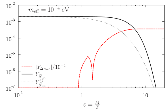
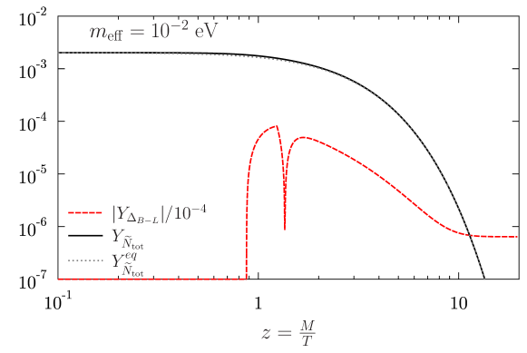
Figure 5: Evolution of $Y_{\widetilde{N}_{\rm tot}}$ (black solid curve) and $Y_{\Delta_{B-L}}$ (red dashed curve) assuming an initial thermal RHSN abundance $Y^{0}_{\widetilde{N}_{\rm tot}}=2Y_{\widetilde{N}}^{eq0}$ for $m_{\rm eff}=10^{-4}\,{\rm eV}$ (top) and $m_{\rm eff}=10^{-2}\,{\rm eV}$ (bottom). The equilibrium RHSN abundance $Y_{\widetilde{N}_{\rm tot}}^{eq}$ is given by the gray dotted curve.

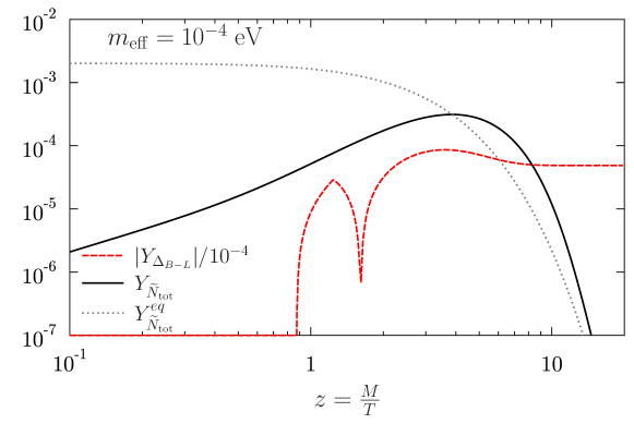
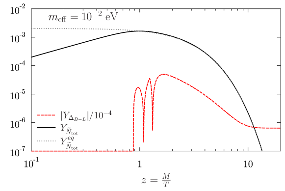
Figure 6: Evolution of $Y_{\widetilde{N}_{\rm tot}}$ (black solid curve) and $Y_{\Delta_{B-L}}$ (red dashed curve) assuming an initial vanishing RHSN abundance, for $m_{\rm eff}=10^{-4}\,{\rm eV}$ (top) and $m_{\rm eff}=10^{-2}\,{\rm eV}$ (bottom). The equilibrium RHSN abundance $Y_{\widetilde{N}_{\rm tot}}^{eq}$ is given by the gray dotted curve.

Notice that with thermal initial RHSN abundance and in the weak washout regime, the efficiency does not flatten out to a maximum value as we would have expected if the CP asymmetry were constant, i.e. temperature independent. What we observe in Fig. 7 is that in this case, $\eta$ (dashed red curve) decreases with decreasing $m_{\rm eff}$ due to the temperature dependence of the CP asymmetry. As $m_{\rm eff}$ decreases and Yukawa interactions become correspondingly weaker, the RHSN decay at a later time (see the top panel of Fig. 5) when the CP asymmetry is smaller (see Fig. 3), and this explains the smaller efficiency. In the strong washout regime, the efficiency decreases with increasing $m_{\rm eff}$ due to increasing washout (see the bottom panel of Fig. 5). If the CP asymmetry were constant, the efficiency would decrease roughly as $\sim 1/m_{\rm eff}$ (see e.g. Ref. Fong:2010a for a discussion of leptogenesis in the strong washout regime). However, larger $m_{\rm eff}$ also shifts towards smaller temperatures the moment when the $B-L$ asymmetry is generated. Because of the strong temperature dependence of the CP asymmetry in SL, this implies that the efficiency decreases faster $\sim 1/m_{\rm eff}$ as can be seen from Fig. 7.

The solid black curve in Fig. 7 shows that with zero initial RHSN abundance, the efficiency $\eta$ quickly drops to zero somewhere around the intermediate washout regime, to rise again for larger values of $m_{\rm eff}$. This corresponds to a change of sign in the ratio $Y_{\Delta_{B-L}}^{\infty}/\bar{\epsilon}$ that occurs for the following reason: during the RHSN production phase (i.e. $Y_{\widetilde{N}_{\rm tot}}<2Y_{\widetilde{N}}^{eq}$), the “wrong” sign lepton asymmetry is generated. In the weak washout regime, a large part of “wrong” sign asymmetry survives because the washouts are weak and also because the “right” sign asymmetry is generated at later times when the CP asymmetry is smaller. As a result, the “right” sign asymmetry cannot overcome the “wrong” sign one (see the top panel of Fig. 6). In the strong washout regime, the washout of the initial “wrong” sign lepton asymmetry is more efficient and also the RHSN will decay earlier when the CP asymmetry is larger. The combination of these two effects results in a final “right” sign lepton asymmetry (see the bottom panel of Fig. 6). In the intermediate regime, a perfect cancellation between the “wrong” and “right” sign lepton asymmetries occurs in the dip observed in Fig. 7 where the efficiency vanishes.

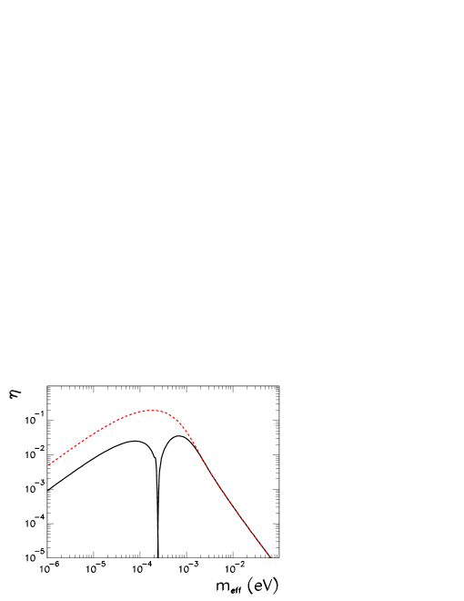
Figure 7: Efficiency factor $\eta$ as a function of $m_{\rm eff}$ for $M=10^{7}$ GeV and $\tan\beta=30$, and for vanishing (solid black curve) and thermal initial RHSN abundance (dashed red curve).

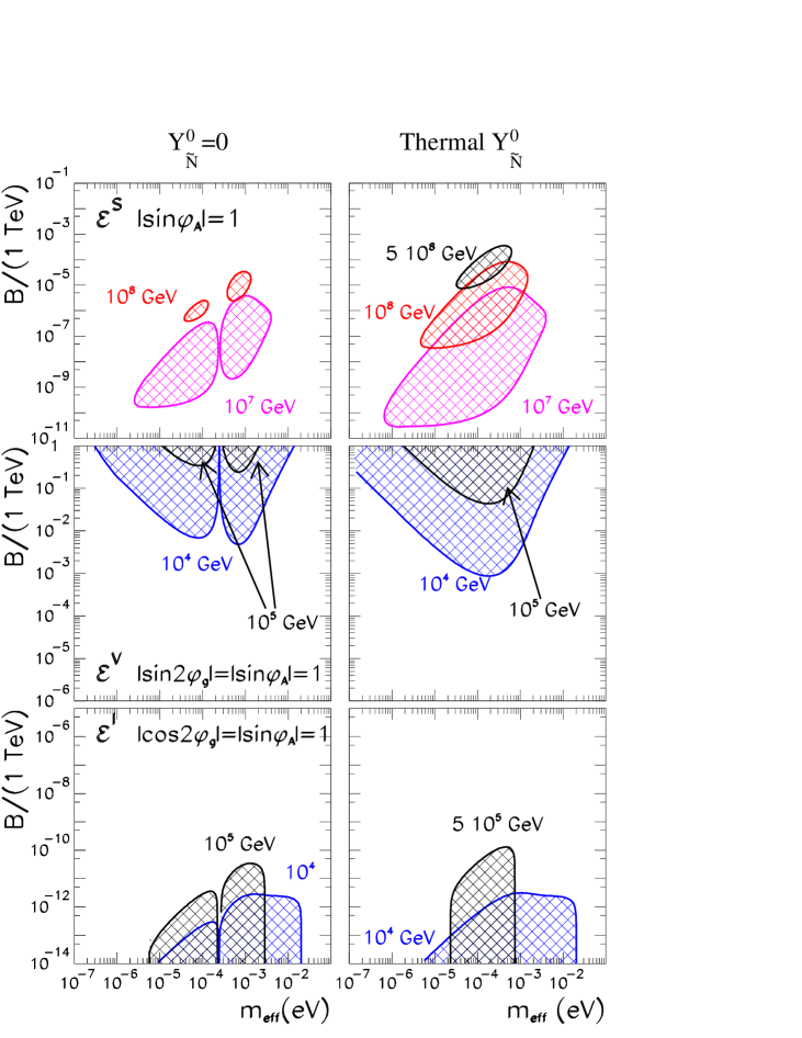
Figure 8: $B,m_{\rm eff}$ regions in which successful SL can be achieved (flavour and spectator effects neglected). In all cases we take $A=m_{2}=10^{3}$ GeV and $\tan\beta=30$ and different values of $M$ and $\phi_{A}$ and $\phi_{g}$ as labeled in the figure (see text for details). The left (right) panels correspond to vanishing (thermal) initial $\widetilde{N}$ abundance .

The upper panels in Fig. 8 show the regions of parameters for which CP violation from pure mixing effects ($\epsilon^{S}$) can produce the observed asymmetry. Due to the resonant nature of this contribution, these effects are sufficiently large only when $B\sim{\cal O}(\Gamma)$ which, as discussed in the the original proposals of SL,[50, 51] implies unconventionally small values of $B$ and an upper bound $M\lesssim 10^{9}\,$GeV.

The central panels of Fig. 8 give the corresponding regions for which CP violation from gaugino-induced vertex effects ($\epsilon^{V}$) can produce the observed baryon asymmetry. Despite being higher order in $\delta_{S}$ and proportional to the square of the gauge couplings ($\alpha_{2}$), this contribution can be relevant because it dominates for conventional values of the $B$ parameter. However, in order to overcome the $\delta_{S}$ and $\alpha_{2}$ suppression this contribution can only be sizable if the RHSN are light $M\lesssim\;10^{6}$ GeV (with the approximation used in this work: $\delta_{S}\ll 1$, $A,m_{2}\sim{\cal O}({\rm TeV})$).

The figure corresponds to values of the parameters such that the second term in Eq.(55) dominates, so that the allowed region depicts a lower bound on $B$. Conversely, when the first term in Eq.(52) dominates, $\epsilon^{V}$ becomes independent of $B$. In this case, for a given value of $M$ and $\delta_{S}$ the produced baryon asymmetry can be sizable within the range of $m_{\rm eff}$ values for which $\eta$ is large enough. For example for $M=10^{5}$ GeV, and $m_{2}=A=1$ TeV and $|\sin(\phi_{A}+2\phi_{g})=1|$ with vanishing initial conditions

$$10^{-5}<\frac{m_{\rm eff}}{\rm eV}<6.5\times 10^{-4}\;\;\;\;\;\;\;{\rm or}\;\;\;\;\;\;8\times 10^{-4}<\frac{m_{\rm eff}}{\rm eV}<3\times 10^{-2},$$ (124)

where each range corresponds to a sign of the CP phase $\sin(\phi_{A}+2\phi_{g})$

Finally we show in the lower panels of Fig. 8 the values of $B$ and $m_{\rm eff}$ for which enough baryon asymmetry can be generated from the interference of mixing and vertex corrections $\epsilon^{I}$ in Eq.(53). Generically speaking, $\epsilon^{I}$ is subdominant with respect to $\epsilon^{S}$, since both involve the same CP phase $\sin(\phi_{A})$ but $\epsilon^{I}$ has additional $\delta_{S}$ and $\alpha_{2}$ suppression:

$$\frac{\bar{\epsilon}^{I}}{\bar{\epsilon}^{S}}=-\frac{3}{8}\alpha_{2}\frac{m_{2}}{M}\ln\frac{m_{2}^{2}}{M^{2}+m_{2}^{2}}\cos(2\phi_{g})\frac{\Gamma}{B}\;.$$ (125)

Consequently, as it is also shown by the figure, $\epsilon^{I}$ can dominate only if $B$ is extremely small ($B\ll\Gamma$), when it becomes independent of $B$. Note also that for $M\lesssim 10^{4}\,$GeV and $m_{\rm eff}\gtrsim 10^{-2}\,$eV the baryon asymmetry generated by this contribution becomes independent of $m_{\rm eff}$. This is because in this regime of strong washouts the $m_{\rm eff}^{2}$ dependence from $\Gamma^{2}$ cancels the approximate $1/m_{\rm eff}^{2}$ dependence of $\eta$.

4 The Possible Role of Quantum Effects

Most studies of thermal leptogenesis (both for the standard seesaw case, as well as for the SL scenario) rely on the classical BE approach that was described in the previous section. The possibility of using quantum BE (QBE) in leptogenesis was first discussed in Ref. Buchmuller:2000, and more recently analyzed in greater detail in Refs. DeSimone:2007b,Anisimov:2010aq,Anisimov:2010dk,Garny:2009rv,Garny:2009qn,Cirigliano:2009yt,Beneke:2010dz. In Ref. DeSimone:2007b, QBE were obtained starting from the non-equilibrium quantum field theory based on the Closed Time-Path (CTP) formulation, and differ from the classical BE in that they contain integrals over the past times. In the classical kinetic theory instead the scattering terms do not include any integral over the past history of the system, which is equivalent to assuming that any collision in the plasma is independent of the previous ones. In the CTP formalism, the energy conservation delta functions appearing in the evaluation of the reaction rates are substituted by retarded time integrals of time-dependent kernels, and cosine functions whose arguments are the energy involved in the reactions. In the limit in which the time range of the kernels is shorter than the relaxation time of the particle abundances, and the time integrals are taken over an infinite time (i.e. neglecting memory effects), the standard time-independent reaction rates are recovered. Furthermore, the CP asymmetry also acquires an additional time-dependent piece, that at any given instant depends upon the previous history of the system.

In Ref. DeSimone:2007b it was argued that the additional time dependence of the CP asymmetry is quantitatively the most relevant effect for leptogenesis. However, if the time variation of the CP asymmetry is shorter than the relaxation time of the particles abundances, the solutions to the quantum and the classical Boltzmann equations are expected to differ only by terms of the order of the ratio of the time-scale of the CP asymmetry to the relaxation time-scale of the distribution. This is typically the case in thermal leptogenesis with hierarchical RHN. Conversely in the resonant leptogenesis scenario, $(M_{j}-M_{i})$ is of the order of the decay rate of the RH neutrinos. As a consequence the typical time-scale to build up coherently the time-dependent CP asymmetry, which is of the order of $(M_{j}-M_{i})^{-1}$, can be larger than the time-scale for the change of the abundance of the RHN. As shown in Refs. DeSimone:2007c,Cirigliano:2008, in the case of resonant leptogenesis this leads to quantitative differences between the classical and quantum approach and, in particular, in the weak washout regime this can enhance the produced asymmetry.

Since in SL the CP asymmetry in mixing (Eq. (51)) is produced resonantly, we can expect that this type of effects could be of some relevance.[106]

4.1 Modification to the CP asymmetry and quantification

We have seen in Section 2.2 that the relevant CP asymmetry in SL is temperature (i.e. time) dependent already in the classical approximation. The inclusion of quantum effects introduces an additional time dependence. As shown in Refs. DeSimone:2007b,DeSimone:2007c,Cirigliano:2008 quantum effects are flavour independent as long as the damping rates of the leptons are taken to be flavour independent. Neglecting also the difference in the width of the two RHSN, one can show that

$$\epsilon^{S}(T)=\bar{\epsilon}^{S}\,\times\,\Delta_{BF}(T)\,\times\,QC(t),$$ (126)

where $\bar{\epsilon}^{S}$ is defined in Eq. (54) and

$$QC(t)=2~{}\sin^{2}\left(\frac{M_{+}-M_{-}}{2}t\right)-\frac{\Gamma}{M_{+}-M_{-}}~{}\sin\left((M_{+}-M_{-})t\right).$$ (127)

The factor $QC(t)$ is the one that remains after taking the past time integral to large time such that only on-shell decay processes contribute to the CP asymmetry (which is equivalent to neglecting memory effects in decay processes). This factor grows for $t\lesssim 1/\Delta M$ and starts oscillating for $t\gtrsim 1/\Delta M$. The oscillation pattern originates from the CP-violating decays of two mixed states $N_{+}$ and $N_{-}$ analogous to the CP violation in neutral meson systems. If the timescale for the decay $\,t\sim 1/\Gamma\,$ is much larger than $1/\Delta M$, the CP asymmetry should average to the classical value. However, if the decay timescale $t\sim 1/\Gamma$ is shorter than $1/\Delta M$, this additional time dependence on CP asymmetry may not be negligible.

As usual, it is convenient to change in Eq. (127) from time $t$ to $z=M/T$. For a Universe undergoing adiabatic expansion the entropy per comoving volume is constant, i.e. $sR^{3}=$ constant, and since $s\propto z^{-3}$ then $R\propto z$. Thus the Hubble parameter is given by $H\equiv R^{-1}dR/dt=z^{-1}dz/dt$. After integration, one gets

$$t=\frac{1}{H(M)}\frac{z^{2}-z_{0}^{2}}{2},$$ (128)

where $z_{0}$ is the temperature at $t=0$. Substituting Eq. (128) into Eq. (127):

$$QC(z) = 2~{}\sin^{2}\left(\frac{1}{2}\frac{M_{+}-M_{-}}{2H(M)}z^{2}\right)-\frac{\Gamma}{M_{+}-M_{-}}~{}\sin\left(\frac{M_{+}-M_{-}}{2H(M)}z^{2}\right),$$ (129)

$$= 2\sin^{2}\left(\frac{m_{\rm eff}}{m^{*}}\,R\,\frac{z^{2}}{8}\right)-\frac{2}{R}\sin\left(\frac{m_{\rm eff}}{m^{*}}\,R\,\frac{z^{2}}{4}\right),$$

where $z_{0}$ has been set equal to $0$ (corresponding to a very high initial temperature) and $M_{+}-M_{-}=B$ has been used (assuming $\widetilde{M}\ll M$ (see Eq. (15)). Finally, the degeneracy parameter $R$ has been defined as:

$$R=\frac{2(M_{+}-M_{-})}{\Gamma}=\frac{2B}{\Gamma}.$$ (130)

In summary, the final CP asymmetry consists of three factors: the first one is the temperature independent piece $\,\bar{\epsilon}^{S}$ which can be rewritten as

$$\bar{\epsilon}^{S}=\frac{{\rm Im}A}{M}\frac{2R}{R+1}.$$ (131)

which, as discussed before, it is resonantly enhanced for $R=1$. The second one is the thermal factor $\Delta_{BF}(T)$ which is non-vanishing only for $z\gtrsim 0.8$ (see Fig. 3). The third one is the quantum correction factor $QC(z)$.

The impact of this additional quantum time-dependence of the CP asymmetry on the final baryon asymmetry can be easily quantified by introducing $QC(z)$ in the relevant BE (110), (111) and (112). Fig. 9 shows the evolution of the asymmetry with and without the inclusion of the quantum correction factor for several values of the washout parameter $m_{\rm eff}$ both for the resonant case $R=1$ and for the very degenerate case $R=2\times 10^{-4}$. The two upper panels correspond to strong and moderate washout regimes, while the lower two correspond to weak and very weak washout regimes.

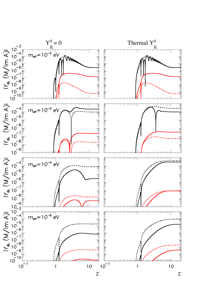
Figure 9: Absolute value of the lepton asymmetry with the quantum time dependence of the CP asymmetry (solid) and without it (dashed) as a function of $z$ for different values of $m_{\rm eff}$ as labeled in the figure. In each panel the two upper curves (black) correspond to the resonant case $R=1$ while the lower two curves (red) correspond to the very degenerate case $R=2\times 10^{-4}$. The left (right) panels correspond to vanishing (thermal) initial RHSN abundance. The figure corresponds to $M=10^{7}$ GeV and $\tan\beta=30$.

The figure illustrates that, as expected, for strong washouts and large degeneracy parameter $R$ (see the upper curves in the upper panels), the quantum effects lead to an oscillation of the produced asymmetry until it averages out to the classical value. Conversely, for very small values of $R$ and strong washouts, quantum effects enhance the final asymmetry. For small enough $R$ the arguments in the periodic functions in $QC(z)$ are very small for all relevant values of $z$ and $m_{\rm eff}$, so that the $\sin^{2}$ term is negligible. By expanding the $\sin$ term we get

$$QC(z)\simeq-\frac{m_{\rm eff}}{m_{*}}\frac{z^{2}}{2},$$ (132)

which, in the strong washout regime, is always larger than 1.

In the weak washout regime, independently of the initial conditions and of the value of the degeneracy parameter $R$, the quantum effects always lead to a suppression of the final asymmetry. This is different from what happens in type I seesaw resonant leptogenesis in which for weak washouts, $R\sim 1$, and vanishing RHN initial abundances, quantum effects lead to an enhancement of the asymmetry produced.[104] The origin of the difference is in the additional time dependence of the CP asymmetry in SL $\Delta_{BF}$. In order to understand how this works, we must remember that in the weak washout regime for type I seesaw resonant leptogenesis, the resulting asymmetry is the one that survives the cancellation between the opposite sign asymmetry generated when RH neutrinos are initially produced, and the asymmetry generated when they decay. Including the time-dependent quantum corrections spoils this cancellation and as a consequence a larger asymmetry is obtained.[104]

However, in SL already in the classical approximation the thermal factor $\Delta_{BF}$ prevents the opposite sign asymmetries cancellation, and the inclusion of the time dependent quantum effects only amounts to an additional multiplicative factor which, in this regime, is smaller than one. Consequently, for SL, even in the resonant-regime quantum effects do no lead to major quantitative differences, at least in the range of parameters for which successful leptogenesis is possible. This is explicitly shown in Fig. 10 that depicts the ranges of the parameters $B$ and $m_{\rm eff}$ for which enough asymmetry is generated ($Y_{\Delta B}^{\infty}\geq 8.35\times 10^{-11}$), with and without the inclusion of the quantum corrections. We see that the main effect of including quantum corrections is that for a given value of $M$ the allowed regions extend up to larger values of $m_{\rm eff}$. This is precisely due to the suppression of the asymmetry in the weak washout regime just discussed. Because of the enhancement in the very degenerate, strong washout regime, for a given value of $M$ the regions also tend to extend to lower values of $B$ and larger values of $m_{\rm eff}$.

A qualitative difference obtained from the inclusion of quantum effects is that, depending on the value of $m_{\rm eff}$, $\eta$ can take both signs independently of the initial RHSN abundance. Thus it is possible to generate the right sign asymmetry with either sign of ${\rm Im}A$ for both thermal and zero initial RHSN abundance. However, apart from this peculiarity, altogether it can be concluded that for a given $M$ the values of the $L$-violating soft bilinear term $B$ required to achieve successful leptogenesis are not substantially modified.

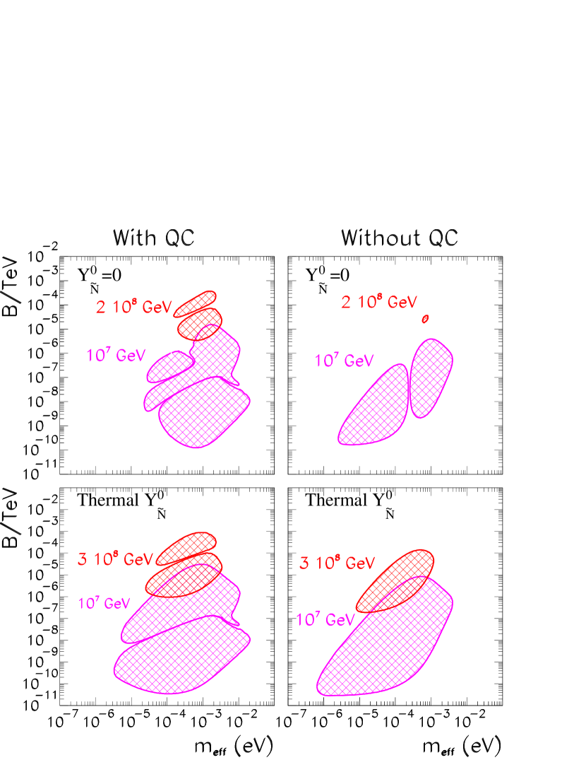
Figure 10: $B,m_{\rm eff}$ regions in which successful SL can be achieved with (left panels) and without (right panels) quantum effects. We take $|{\rm Im}A|=10^{3}$ GeV and $\tan\beta=30$ and different values of $M$ as labeled in the figure. The upper (lower) panels correspond to vanishing (thermal) initial RHSN abundance.

5 The Role of Lepton Flavours

The role of lepton flavour in the standard thermal leptogenesis scenario was first discussed in Ref. Barbieri:2000. However, until the importance of flavour effects was fully clarified[63, 64] they had been included in leptogenesis studies only in a few cases.[62, 107] Nowadays flavour effects have been investigated in full detail[65, 108, 109, 110, 111, 112, 113, 114, 115, 97, 104, 105, 71] and are a mandatory ingredient of any reliable analysis of leptogenesis.

As regards SL, the original works[50, 51] neglected flavour effects and considered the generation of the lepton asymmetry directly in the $\ell$ and $\widetilde{\ell}$ lepton states coupled to the lightest RHSN, a situation commonly referred to as the ‘one flavour approximation’. However, RHSN couple in fact to certain lepton combinations, in which the different flavours are weighted by the respective RHN Yukawa couplings: $\ell\propto\sum_{\alpha}Y_{\alpha}\ell_{\alpha}$ and $\widetilde{\ell}\propto\sum_{\alpha}Y_{\alpha}\widetilde{\ell}_{\alpha}$. Only at very high temperatures $\ell$ and $\widetilde{\ell}$ remain coherent superpositions, and are the correct states to describe the dynamics of leptogenesis. At lower temperatures scatterings induced by the charged lepton Yukawa couplings occur at a sufficiently fast pace to distinguish the different lepton flavour components. In this situation, $\ell$ and $\widetilde{\ell}$ cannot be considered anymore as coherent flavour superpositions, and the dynamics of leptogenesis must be described instead in terms of the flavour eigenstates $\ell_{\alpha}$ and $\widetilde{\ell}_{\alpha}$. The specific temperature when leptogenesis becomes sensitive to lepton flavour dynamics can be estimated by requiring that the rates of processes $\Gamma_{\alpha}$ ($\alpha=e,\mu,\tau$) that are induced by the charged lepton Yukawa couplings $h_{\alpha}$ become faster than the Universe expansion rate $H(T)$. An approximate relation gives[116, 117]

$$\Gamma_{\alpha}(T)\simeq 10^{-2}h_{\alpha}^{2}T\,,$$ (133)

which implies that

$$\Gamma_{\alpha}(T)>H(T)\qquad{\rm when}\qquad T\lesssim T_{\alpha}\,(1+\tan\beta^{2})\,,$$ (134)

where $T_{e}\simeq 4\times 10^{4}\,$GeV, $T_{\mu}\simeq 2\times 10^{9}\,$GeV, and $T_{\tau}\simeq 5\times 10^{11}\,$GeV. Notice that to fully distinguish the three flavours it is sufficient that the $\tau$ and $\mu$ Yukawa reactions attain thermal equilibrium. Therefore, given that SL can successfully proceed only for temperatures below $T_{\mu}$, we can conclude that independently of the value of $\tan\beta$ the three flavour regime is always the appropriate one to study SL. The interesting issue is if the region of parameter space in which SL can be successful is enlarged or reduced when flavour effects are taken into account, and in particular if the requirement of unnaturally small values of the soft $B$ term can get relaxed. These issues are addressed in the following sections.

5.1 Flavored CP asymmetries

In the flavour regime the CP asymmetries for RHSN decays into the single lepton flavours become important. Their flavour structure is determined by the Yukawa couplings $Y_{\alpha}$ as well as by the trilinear couplings $A_{\alpha}$. The soft breaking Lagrangian of the previous section Eq. (12) assumed for simplicity a universal trilinear soft breaking scale $A$ and proportionality of the soft breaking trilinear couplings to the Yukawa couplings, that is $A_{\alpha}=AY_{\alpha}$. In this section a more general flavour structure is considered where the $A$-terms have the generic flavour structure

$$-\mathcal{L}_{\rm soft}^{(A)}=AZ_{i\alpha}\,\epsilon_{ab}\widetilde{N}_{i}\widetilde{\ell}_{\alpha}^{a}H_{u}^{b}+{\rm h.c.}\,.$$ (135)

Considering only the lightest RHSN $\widetilde{N}=\widetilde{N}_{1}$ and adopting as usual a simplified notation $Z_{\alpha}=Z_{1\alpha}$ etc., with the generalized flavour configuration in Eq. (135) we have three relevant physical phases:

$$\phi_{A_{\alpha}}=\arg(AZ_{\alpha}Y_{\alpha}^{*}B^{*}).$$ (136)

and the CP asymmetries (51),(52) and (53) are now written as:

$$\epsilon_{\alpha}^{S,V,I}(T)=P_{\alpha}\,\frac{Z_{\alpha}}{Y_{\alpha}}\,\bar{\epsilon}^{S,V,I}_{\alpha}\,\Delta_{BF}(T),$$ (137)

where

$$\bar{\epsilon}_{\alpha}^{S}\equiv-\frac{A}{M}\sin\left(\phi_{A_{\alpha}}\right)\frac{4B\Gamma}{4B^{2}+\Gamma^{2}}$$ (138)

$$\bar{\epsilon}_{\alpha}^{V}\equiv-\frac{3\alpha_{2}}{4}\frac{m_{2}}{M}\ln\frac{m_{2}^{2}}{m_{2}^{2}+M^{2}}\left[\frac{A}{M}\sin\left(\phi_{A_{\alpha}}+2\phi_{g}\right)-\frac{Y_{\alpha}}{Z_{\alpha}}\frac{B}{M}\sin\left(2\phi_{g}\right)\right],\quad\ \$$ (139)

$$\bar{\epsilon}_{\alpha}^{I}\equiv\frac{3\alpha_{2}}{2}\frac{m_{2}}{M}\frac{A}{M}\ln\frac{m_{2}^{2}}{m_{2}^{2}+M^{2}}\sin\left(\phi_{A_{\alpha}}\right)\cos\left(2\phi_{g}\right)\frac{\Gamma^{2}}{4B^{2}+\Gamma^{2}}\,.$$ (140)

In these equations the physical complex phases $\phi_{A_{\alpha}}$ and $\phi_{g}$ have been explicitly written, so that all the parameters $A$, $Z_{\alpha}$, $Y_{\alpha}$ etc. are real and positive. Unless explicitly stated in the text, this convention is adopted also in what follows. As regards the flavoured reaction rates, they can be simply written in terms of the unflavoured rates by means of the flavour projectors Eq. (49):

$$\gamma_{X}^{\alpha}=P_{\alpha}\gamma_{X}\;.$$ (141)

5.2 Flavour structures

The flavour structure $Z_{\alpha}$ of the $A$ terms Eq. (135) is in principle independent from the flavour structure of the Yukawa couplings $Y_{\alpha}$. However, the study of flavour effects in a completely general flavour configuration would be rather awkward, because of the very large dimensionality of the parameter space. It is thus convenient to define less general possibilities, but chosen in such a way to render possible a qualitative extrapolation of the impact of flavour effects to the general case. In Refs. Fong:2008a and Fong:2010zu the following two scenarios were respectively introduced:

1. Universal Trilinear Scenario (UTS).[118] This case assumes universal soft terms, that is the soft breaking Lagrangian of Eq. (12). It is realized in supergravity or gauge mediation (when the renormalization group running of the parameters is neglected) and corresponds to set

$$Z_{\alpha}=Y_{\alpha}.$$ (142)

Thus, in UTS the only flavour structure arises from the Yukawa couplings and both the flavoured total CP asymmetries $\epsilon_{\alpha}=\epsilon^{S}_{\alpha}+\epsilon^{V}_{\alpha}+\epsilon^{I}_{\alpha}$ and the flavoured washout terms $W_{\alpha}$ are proportional to the same flavour projectors $P_{\alpha}$. It follows that $\epsilon_{\alpha}\propto W_{\alpha}$, and moreover, as seen in Eq. (136), the trilinear couplings have an unique phase $\phi_{A_{\alpha}}=\phi_{A}=\arg(AB^{*})$.

2. Simplified Misaligned Scenario (SMS).[119] To understand the possible effects of flavour dynamics, it is important to study also a case in which the flavoured CP asymmetries $\epsilon_{\alpha}$ and the washouts $W_{\alpha}$ are misaligned. This can be done without increasing the number of independent parameters with respect to UTS by imposing the condition[119]

$$Z_{\alpha}=\frac{\displaystyle\sum_{\beta}|Y_{\beta}|^{2}}{3Y^{*}_{\alpha}}\;,$$ (143)

where we have kept $Z$ and $Y$ explicitly as complex numbers. With this condition the CP asymmetries (except for the last term in Eq. (139)) are equal for all flavours $\epsilon_{\alpha}=\epsilon/3$, while the washouts $W_{\alpha}$ maintain their flavour dependence, so that an arbitrary misalignment can be realized. From Eq. (136) we see that there is again a unique phase $\phi_{A_{\alpha}}=\phi_{A}=\arg(AB^{*})$. Note that both Eq.(142) and Eq. (143) yield the same total asymmetry $\sum_{\alpha}\epsilon_{\alpha}=\epsilon$, so that any difference between the UTS and SMS results can be ascribed directly to the differences in flavour configuration. Note also that in the case of flavour equipartition $P_{e}=P_{\mu}=P_{\tau}=1/3$ the two scenarios are equivalent.

Finally, it should be remarked that in both scenarios it is not possible to have flavour asymmetries of opposite signs, with $|\epsilon^{\alpha}|>|\epsilon|$ for some, or even for all flavours, as it is also excluded the possibility of having non-zero flavour asymmetries and a vanishing total CP asymmetry. This however, is simply due to the reduction in the number of physical phases and, similarly to what happens in standard flavoured leptogenesis,[63, 64, 65] in the most general case asymmetries of opposite signs (and possibly with a vanishing sum) are an open possibility. Given that these types of configurations are always characterized by larger CP asymmetries, the reader should keep in mind that enhancements of the final lepton asymmetry even larger than the ones found in UTS and SMS are certainly possible.

5.3 Lepton flavour equilibration

The possibility of having large enhancements of the baryon asymmetry yield of leptogenesis from flavour effects, relies on the fact that the density asymmetries stored in each flavour are independent from each other, and if for example a flavour that is weakly coupled to the washouts has a particularly large CP asymmetry, the final result will be essentially determined by the dynamics of this flavour.

However, in the presence of lepton flavour violating (LFV) interactions, the density asymmetries in the different flavours are no more independent, and if LFV rates are sufficiently fast, they can bring the different flavours into equilibrium, with the result that the amount of surviving asymmetry will be essentially determined by the flavour that is more strongly washed out: a potentially destructive effect.[120]

In SL, LFV interactions are a natural possibility since they are directly related to off-diagonal entries in the soft mass matrices of the sleptons. For this reason a reliable study of flavoured SL must also include an analysis of LFV effects.

In the basis where charged lepton Yukawa couplings are diagonal, the soft slepton masses read

$$\mathcal{L}_{soft} \supset -\widetilde{m}_{\alpha\beta}^{2}\widetilde{\ell}_{\alpha}^{*}\widetilde{\ell}_{\beta}.$$ (144)

The off-diagonal soft slepton masses $\widetilde{m}_{\alpha\neq\beta}^{2}\equiv\widetilde{m}_{\alpha\beta}^{2}\,\;(\alpha\neq\beta)$ affect the flavour composition of the slepton mass eigenstates so generically we can write

$$\widetilde{\ell}_{\alpha}^{\left(int\right)}=R_{\alpha\beta}\widetilde{\ell}_{\beta},$$ (145)

where $R_{\alpha\beta}$ is a unitary rotation matrix. In this basis the corresponding slepton-gaugino interactions in Eq. (16) become

$$-\mathcal{L}_{\widetilde{\lambda},\widetilde{\ell}} = g_{2}\left(\sigma_{\pm}\right)_{ab}\overline{\widetilde{\lambda}_{2}^{\pm}}P_{L}\ell_{\alpha}^{a}R^{*}_{\alpha\beta}\widetilde{\ell}_{\beta}^{b*}+\frac{g_{2}}{\sqrt{2}}\left(\sigma_{3}\right)_{ab}\overline{\widetilde{\lambda}_{2}^{0}}P_{L}\ell_{\alpha}^{a}R_{\alpha\beta}^{*}\widetilde{\ell}_{\beta}^{b*}$$ (146)

$$+\frac{g_{Y}}{\sqrt{2}}\delta_{ab}\overline{\widetilde{\lambda}_{1}}Y_{\ell L}P_{L}\ell_{\alpha}^{a}R^{*}_{\alpha\beta}\widetilde{\ell}_{\beta}^{b*}\,+\,{\rm h.c.}\;,$$

The mixing matrix can be expressed in terms of the off-diagonal slepton masses as:

$$R_{\alpha\beta} \sim \delta_{\alpha\beta}+\frac{\widetilde{m}_{\alpha\neq\beta}^{2}}{h_{\alpha}^{2}T^{2}}=\delta_{\alpha\beta}+\frac{\widetilde{m}_{\alpha\neq\beta}^{2}v^{2}\cos^{2}\beta}{m_{\alpha}^{2}M^{2}}z^{2},$$ (147)

where in the first line $h_{\alpha}>h_{\beta}$ is the relevant charged Yukawa coupling that determines at leading order the thermal mass splittings of the sleptons, $v$ in the second line is the EW symmetry breaking VEV with $v^{2}=v^{2}_{u}+v^{2}_{d}\simeq 174\,$GeV, $z\equiv\frac{M}{T}$ and $m_{\alpha}\equiv m_{\ell_{\alpha}}(T\!=\!0)$ is the zero temperature mass for the lepton $\ell_{\alpha}$. For simplicity we parametrize the $R_{\alpha\neq\beta}$ entries in a way that they are independent of the particular pair of leptons involved. Let us define $\widetilde{m}_{e\tau}=\widetilde{m}_{\mu\tau}=\widetilde{m}_{od}$ and $\widetilde{m}_{e\mu}=\widetilde{m}_{od}\frac{m_{\mu}}{m_{\tau}}$, where $\widetilde{m}_{od}$ is a unique off-diagonal soft-mass parameter. We then obtain for the off-diagonal entries $(\alpha\beta)=(e\tau),\,(\mu\tau),\,(e\mu)$ of the matrix $R$:

$$R_{\alpha\neq\beta} \sim \frac{\widetilde{m}_{od}^{2}\,v^{2}\cos^{2}\beta}{m_{\tau}^{2}M^{2}}\,z^{2},$$ (148)

where $m_{\tau}$ is the mass of the tau lepton.

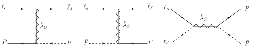
Figure 11: LFV lepton-slepton scatterings mediated by the $SU(2)_{L}$ and $U(1)_{Y}$ gauginos $\widetilde{\lambda}_{G}$.

The terms in Eq. (146) induce LFV lepton-slepton scatterings through the exchange of $SU(2)_{L}$ and $U(1)_{Y}$ gauginos.[120] There are two possible t-channel scatterings $\,\ell_{\alpha}\overline{P}\leftrightarrow\widetilde{\ell}_{\beta}\widetilde{P}^{*}$, $\,\ell_{\alpha}\widetilde{P}\leftrightarrow\widetilde{\ell}_{\beta}P$ and one s-channel scattering $\,\ell_{\alpha}\widetilde{\ell}_{\beta}^{*}\leftrightarrow P\widetilde{P}^{*}$ (we denote $P$ as fermions and $\widetilde{P}$ as scalars) as shown in Fig. 11. For processes mediated by $SU(2)_{L}$ gauginos $P=\ell,Q,\widetilde{H}_{u,d}$, while when mediated by $U(1)_{Y}$ gaugino one must include the $SU(2)_{L}$ singlet states $P=e,u,d$ as well. The corresponding reduced cross sections read:

$$\hat{\sigma}_{t1,G}^{\alpha\beta}\left(s\right) = {\displaystyle\sum_{P}}\frac{g_{G}^{4}\left|R_{\alpha\beta}\right|^{2}\Pi_{P}^{G}}{8\pi}\left[\left(\frac{2m_{\widetilde{\lambda}_{G}}^{2}}{s}+1\right)\ln\left|\frac{m_{\widetilde{\lambda}_{G}}^{2}+s}{m_{\widetilde{\lambda}_{G}}^{2}}\right|-2\right],$$

$$\hat{\sigma}^{\alpha\beta}_{t2,G}\left(s\right) = {\displaystyle\sum_{P}}\frac{g_{G}^{4}\left|R_{\alpha\beta}\right|^{2}\Pi_{P}^{G}}{8\pi}\left[\ln\left|\frac{m_{\widetilde{\lambda}_{G}}^{2}+s}{m_{\widetilde{\lambda}_{G}}^{2}}\right|-\frac{s}{m_{\widetilde{\lambda}_{G}}^{2}+s}\right],$$

$$\hat{\sigma}^{\alpha\beta}_{s,G}\left(s\right) = {\displaystyle\sum_{P}}\frac{g_{G}^{4}\left|R_{\alpha\beta}\right|^{2}\Pi_{P}^{G}}{16\pi}\left(\frac{s}{s-m_{\widetilde{\lambda}_{G}}^{2}}\right)^{2}\;,$$ (149)

where $\Pi_{P}^{G}$ counts the numbers of degrees of freedom of the particle $P$ (isospin, quark flavours and color) involved in the scatterings mediated by the $SU(2)_{L}$ ($G=2$) and $U(1)_{Y}$ ($G=Y$) gauginos respectively. In this last case the hypercharges $y_{\ell L}$ and $y_{P}$ are also included in $\Pi_{P}^{Y}$. If the flavour changing scatterings in Eq. (149) are fast enough, they will lead to lepton flavour equilibration (LFE).[120]

The values of $\widetilde{m}_{od}$ for which this occurs can be estimated by comparing the LFE scattering rates and the $\Delta L=1$ washout rates. Since the dominant $\Delta L=1$ contribution arises from inverse decays, the terms to be compared are:

$$\overline{\Gamma}_{\rm LFE}(T)\equiv\frac{\gamma_{\rm LFE}(T)}{n^{c}_{L}(T)},\qquad\qquad\overline{\Gamma}_{\rm ID}(T)\equiv\frac{\gamma_{\tilde{N}}(T)}{n^{c}_{L}(T)}\,,$$ (150)

where $n^{c}_{L}=T^{3}/2$ is the relevant density factor appearing in the washouts (see next section for more details) and

$$\gamma_{\rm LFE}(T) = {\displaystyle\sum_{G,P}}\Pi^{G}_{P}(\gamma^{\alpha\beta}_{t1,G}+\gamma^{\alpha\beta}_{t2,G}+\gamma^{\alpha\beta}_{s,G})$$ (151)

$$= \frac{T}{64\pi}{\displaystyle\sum_{G}}\int ds\sqrt{s}{\cal K}_{1}\left(\frac{\sqrt{s}}{T}\right)\,\left[\hat{\sigma}^{\alpha\beta}_{t1,G}(s)+\hat{\sigma}^{\alpha\beta}_{t2,G}(s)+\hat{\sigma}^{\alpha\beta}_{s,G}(s)\right]\;,$$

$$\gamma_{\tilde{N}}(T) = n_{\tilde{N}}^{eq}(T)\,\frac{{\cal K}_{1}(z)}{{\cal K}_{2}(z)}\,\Gamma\;.$$ (152)

In the first equality in Eq.(151) $\gamma^{\alpha\beta}_{x,G}$ with ($x=t1,t2,s$) is the thermally averaged LFE reactions for one degree of freedom of the $P$-particle, $\mathcal{K}_{1,2}(z)$ are the modified Bessel function of the second kind of order 1 and 2, $\Gamma$ is the zero temperature width Eq. (22), and $n_{\widetilde{N}}^{eq}(T)$ is the equilibrium number density for $\widetilde{N}$ at $T$.

The LFE reaction densities, the Universe expansion rate $H$, and inverse decay rates all have a different $T$ dependence. In particular $\overline{\Gamma}_{\rm LFE}\sim T^{-3}$ and $H(T)\sim T^{2}$, so that once LFE reactions have attained thermal equilibrium ($\overline{\Gamma}_{\rm LFE}\ \hbox to0.0pt{\raise 3.0pt\hbox{$>$}\hss}{\lower 3.0pt\hbox{$\sim$}}\ H$) they will remain in thermal equilibrium also at lower temperatures. In contrast, for inverse decays the rate first increases, and then decreases exponentially $\overline{\Gamma}_{\rm ID}\sim e^{-M/T}$ dropping out of equilibrium at temperatures not much below $T\sim M$. The relevant temperature where we should compare the rates of these interactions is precisely when the condition $\overline{\Gamma}_{\rm ID}\approx H$ is reached, that is when the lepton asymmetry starts being generated from the out-of-equilibrium $\widetilde{N}_{\pm}$ decays. Defining $z_{dec}$ through the condition $\overline{\Gamma}_{\rm ID}(z_{dec})=H(z_{dec})$, LFE is expected to be quite relevant for flavoured leptogenesis when

$$\overline{\Gamma}_{\rm LFE}\left(z_{dec}\right) \geq \overline{\Gamma}_{ID}\left(z_{dec}\right),$$ (153)

since when this condition is satisfied, LFE processes are already in thermal equilibrium at the onset of the out-of-equilibrium decay era.

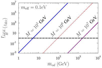
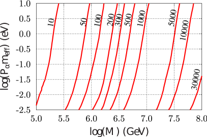
Figure 12: The left panel shows the ratio $\bar{\Gamma}_{\rm LFE}/H$ at $z_{dec}$ as a function of $\widetilde{m}_{od}$ for $m_{\rm eff}=0.1$ eV, $\tan\beta=30$ and three values of $M$. The right panel shows in the ($P_{\alpha}m_{\rm eff},M$) plane contours of constant values of $\widetilde{m}_{od}$ (in GeV) for which $\overline{\Gamma}_{\rm LFE}\left(z_{dec}^{\alpha}\right)\geq P_{\alpha}\overline{\Gamma}_{\rm ID}\left(z_{dec}^{\alpha}\right)$.

The left panel of Fig. 12 shows the ratio $\overline{\Gamma}_{\rm LFE}(z_{dec})/H(z_{dec})$ as a function of $\widetilde{m}_{od}$ for $m_{\rm eff}=0.1$ eV, $\tan\beta=30$, and for different values of $M$. From the figure we can read the characteristic value of $\widetilde{m}_{od}$ for which LFE becomes relevant. Notice that the dominant dependence on $\tan\beta\sim 1/\cos\beta$ ($\tan\beta\gg 1$) arises from $v\cos\beta=v_{d}$ in Eq. (148). Thus the results from other values of $\tan\beta$ can be easily read from the figure by rescaling $\widetilde{m}_{od}(\tan\beta)=\widetilde{m}^{\rm fig}_{od}/(30\cos\beta)$.

Since we are interested in the dynamics of lepton flavours, to be more precise about LFE effects we should in fact consider the temperature at which the inverse decay rate for one specific flavour $\alpha$ goes out of equilibrium. We then define $z_{dec}^{\alpha}$ through the condition $\overline{\Gamma}_{\rm ID}^{\alpha}(z_{dec}^{\alpha})\equiv P_{\alpha}\overline{\Gamma}_{\rm ID}(z_{dec}^{\alpha})=H(z_{dec}^{\alpha})$. For a hierarchical configuration of flavour projectors $P_{\gamma}<P_{\beta}<P_{\alpha}$ we will have $z_{dec}^{\gamma}<z_{dec}^{\beta}<z_{dec}^{\alpha}$, that is the inverse decays involving the lepton doublet $\ell_{\gamma}$ which is the most weakly coupled to $\widetilde{N}_{\pm}$ will go out of equilibrium first, and then $\overline{\Gamma}_{\rm ID}^{\beta}$ and $\overline{\Gamma}_{\rm ID}^{\alpha}$ will follow. Hence, for given values of $m_{\rm eff}$ and $M$, the minimum value $\widetilde{m}_{od}^{min}$ for which LFE effects start being important is given by the following condition:

$$\overline{\Gamma}_{\rm LFE}\left(z_{dec}^{\alpha},\widetilde{m}_{od}^{min}\right) \simeq \overline{\Gamma}_{\rm ID}^{\alpha}\left(z_{dec}^{\alpha}\right).$$ (154)

For $\widetilde{m}_{od}\ll\widetilde{m}_{od}^{min}$ LFE effects can be neglected, since they will attain thermal equilibrium only after leptogenesis is over.

The right panel in Fig. 12 shows in the plane of the flavoured effective decay mass $P_{\alpha}m_{\rm eff}$ and of the RHN mass $M$, various contours corresponding to different values of $\widetilde{m}_{od}$ for which $\overline{\Gamma}_{\rm LFE}\left(z_{dec}^{\alpha}\right)=\Gamma_{\rm ID}^{\alpha}\left(z_{dec}^{\alpha}\right)$. For a given value of $M$ and $m_{\rm eff}$, and for a given set of flavour projections $P_{\gamma}<P_{\beta}<P_{\alpha}$, $\widetilde{m}_{od}^{min}$ is given by the value of the $\widetilde{m}_{od}$ curve for which the vertical line $x=M$ intersects the corresponding contour at $y_{\alpha}=P_{\alpha}\,m_{\rm eff}$. Since $\overline{\Gamma}_{\rm LFE}$ has a rather strong dependence on $\widetilde{m}_{od}$ ($\overline{\Gamma}_{\rm LFE}\propto\widetilde{m}_{od}^{4}$), one expects that the value $\widetilde{m}_{od}^{eq}$ for which LFE effects completely equilibrate the asymmetries in the different lepton flavours will not be much larger than $\widetilde{m}_{od}^{min}$. Indeed our numerical results (see Section 5.7) show that $\widetilde{m}_{od}^{eq}\sim{\cal O}(5-10)\times\widetilde{m}_{od}^{min}$. Clearly, larger values $\widetilde{m}_{od}\gg\widetilde{m}_{od}^{eq}$ do not modify the final results with respect to what is obtained when $\widetilde{m}_{od}=\widetilde{m}_{od}^{eq}$.

5.4 Flavoured Boltzmann equations

In Refs. Barbieri:2000,Abada:2006a,Nardi:2006b the relevant equations including flavour effects associated to the charged lepton Yukawa couplings were derived in the density operator approach. One can define a density matrix for the difference of lepton and antileptons such that $\rho_{\alpha\alpha}=Y_{\Delta\ell_{\alpha}}$. As discussed in Refs. Barbieri:2000,Abada:2006a,Nardi:2006b as long as we are in the regime in which a given set of the charged–lepton Yukawa interactions are out of equilibrium, one can restrict the general equation for the matrix density $\rho$ to a subset of equations for the flavour diagonal directions $\rho_{\alpha\alpha}$. In the transition regimes in which a given Yukawa interaction is approaching equilibrium the off-diagonal entries of the density matrix cannot be neglected.[63, 65, 121] However, as we have discussed, SL always occurs in the three flavour regime, and thus there is no need to worry about this type of effects. In this Section we keep working, as in Section 3, under the assumption of superequilibration. However, we now include the effects of all the relevant fast reactions of type (i) (see Section 3.1) with characteristic time scales much shorter than $H^{-1}(z=1)$, that is we include both flavour and spectator effects. This implies that we need to consider three flavoured lepton density asymmetries that also include the contributions of the $SU(2)_{L}$ singlet (s)leptons, defined as:

$$Y_{\Delta L_{\alpha}}\equiv 2\left(Y_{\Delta\ell_{\alpha}}+Y_{\Delta\widetilde{\ell}_{\alpha}}\right)+Y_{\Delta e_{\alpha}}+Y_{\Delta\widetilde{e}_{\alpha}},$$ (155)

where the factor of 2 comes from summing over the $SU(2)_{L}$ degrees of freedom. The contribution of $e_{\alpha}$ and $\widetilde{e}_{\alpha}$ to the total flavour asymmetries is non-vanishing because scatterings with the Higgs induced by the charged lepton Yukawa couplings transfer part of the asymmetry generated in the $SU(2)_{L}$ lepton doublets to the singlets.

In the BE for the evolution of the RHN and RHSN densities, a sum over flavour can be readily taken, and the resulting equations are not modified with respect to Eqs. (110) and (111). The lepton charges $\Delta L_{\alpha}$ are anomalous, and thus are not only perturbatively violated in RHSN and RHN interactions, but also in nonperturbative sphalerons transitions. This type of effects is however removed by writing evolution equations for the anomaly free flavoured charges $\Delta_{\alpha}\equiv B/3-L_{\alpha}$, with density asymmetries defined as $Y_{\Delta_{\alpha}}\equiv Y_{\Delta B}/3-Y_{\Delta L_{\alpha}}$. Including spectator[83, 84] and LFE[120, 119] effects, the corresponding BE is:

$$-\dot{Y}_{\Delta_{\alpha}} = \epsilon_{\alpha}\left(z\right)\frac{\gamma_{\widetilde{N}}}{2}\left(\frac{Y_{\widetilde{N}_{\rm tot}}}{Y_{\widetilde{N}}^{eq}}-2\right)$$ (156)

$$-\left[\frac{\gamma^{\alpha}_{\widetilde{N}}}{2}+\frac{\gamma^{\alpha}_{N}}{2}+\gamma_{\widetilde{N}}^{\left(3\right)\alpha}+\left(\frac{1}{2}\frac{Y_{\widetilde{N}_{\rm tot}}}{Y_{\widetilde{N}}^{eq}}+2\right)\gamma^{\alpha}_{22}\right]\left({\cal Y}_{\Delta\ell_{\alpha}}+{\cal Y}_{\Delta\widetilde{H}_{u}}\right)$$

$$-2\left(\gamma_{t}^{\left(1\right)\alpha}+\gamma_{t}^{\left(2\right)\alpha}+\gamma_{t}^{\left(4\right)\alpha}+\gamma_{t}^{\left(6\right)\alpha}+\gamma_{t}^{\left(7\right)\alpha}+\gamma_{t}^{\left(9\right)\alpha}\right){\cal Y}_{\Delta\ell_{\alpha}}$$

$$-\left[\left(2\gamma_{t}^{\left(0\right)}+\gamma_{t}^{\left(3\right)\alpha}\right)\frac{Y_{N}}{Y_{N}^{eq}}+\left(\gamma_{t}^{\left(5\right)\alpha}+\frac{1}{2}\gamma_{t}^{\left(8\right)\alpha}\right)\frac{Y_{\widetilde{N}_{\rm tot}}}{Y_{\widetilde{N}}^{eq}}\right]{\cal Y}_{\Delta\ell_{\alpha}}$$

$$-\left(2\gamma_{t}^{\left(0\right)\alpha}+\gamma_{t}^{\left(1\right)\alpha}+\gamma_{t}^{\left(3\right)\alpha}+\gamma_{t}^{\left(4\right)\alpha}+2\gamma_{t}^{\left(5\right)\alpha}\right.\left.+\gamma_{t}^{\left(6\right)\alpha}+\gamma_{t}^{\left(7\right)\alpha}+\gamma_{t}^{\left(8\right)\alpha}+\gamma_{t}^{\left(9\right)\alpha}\right){\cal Y}_{\Delta\widetilde{H}_{u}}$$

$$-\left[\left(\gamma_{t}^{\left(1\right)\alpha}+\gamma_{t}^{\left(2\right)\alpha}+\gamma_{t}^{\left(4\right)\alpha}\right)\frac{Y_{N}}{Y_{N}^{eq}}+\frac{1}{2}\left(\gamma_{t}^{\left(6\right)\alpha}+\gamma_{t}^{\left(7\right)\alpha}+\gamma_{t}^{\left(9\right)\alpha}\right)\frac{Y_{\widetilde{N}_{\rm tot}}}{Y_{\widetilde{N}}^{eq}}\right]{\cal Y}_{\Delta\widetilde{H}_{u}}$$

$$-\sum_{\beta\neq\alpha}\left[84\left(\gamma^{\beta\alpha}_{t1,2}+\gamma^{\beta\alpha}_{t2,2}+\gamma^{\beta\alpha}_{s,2}\right)+76\left(\gamma^{\beta\alpha}_{t1,Y}+\gamma^{\beta\alpha}_{t2,Y}+\gamma^{\beta\alpha}_{s,Y}\right)\right]\left({\cal Y}_{\Delta\ell_{\alpha}}-{\cal Y}_{\Delta\ell_{\beta}}\right),\quad$$

where ${\cal Y}_{\ell_{\alpha}}\equiv Y_{\Delta\ell_{\alpha}}/Y_{\ell}^{eq}$ and ${\cal Y}_{\widetilde{H}_{u}}\equiv Y_{\Delta\widetilde{H}_{u}}/Y_{\widetilde{H}_{u}}^{eq}$ with $Y_{\ell}^{eq}=Y_{\widetilde{H}_{u}}^{eq}=\frac{15}{8\pi^{2}g_{*}}$. Notice that SE implies $2Y_{\Delta\ell_{\alpha}}=Y_{\Delta\widetilde{\ell}_{\alpha}}$ and $2Y_{\Delta\widetilde{H}_{u}}=Y_{\Delta H_{u}}$ and we chose to express the asymmetries in term of the fermionic ones. The higgsino asymmetries enter in two ways: directly, when the Higgs(inos) are involved in the relevant process as external particles, as in RHSN decays and inverse decays; indirectly, when the top and stop quarks are involved in the relevant scatterings, and their chemical potentials are rewritten in terms of $Y_{\Delta\widetilde{H}_{u}}$ (see A.4). The last line in Eq. (156) includes the reaction densities for the LFE processes in Eq. (149), that as discussed above play the role of controlling the effectiveness of flavour effects.

To bring Eq. (156) in the form of a closed differential equations for the charge density asymmetries $Y_{\Delta_{\alpha}}$, the three asymmetries $Y_{\Delta\ell_{\alpha}}$ as well as the higgsino asymmetry $Y_{\Delta\widetilde{H}_{u}}$ must be expressed in terms of $Y_{\Delta_{\alpha}}$ according to:

$$Y_{\Delta\ell_{\alpha}}=\sum_{\beta}A_{\alpha\beta}Y_{\Delta_{\beta}},\qquad\qquad Y_{\Delta\widetilde{H}_{u}}=\sum_{\beta}C_{\beta}Y_{\Delta_{\beta}}.$$ (157)

The matrix $A$ was first introduced in Ref. Barbieri:2000 and the vector $C$ in Ref. Nardi:2006a. The values of their entries are determined by which interactions are in chemical equilibrium, and thus eventually by the specific range of temperature when leptogenesis takes place (see B).

5.5 Results

Unless differently stated, our results are obtained for $M=10^{6}\,$GeV and $\tan\beta=30$, although as long as LFE effects are negligible they are practically independent of $M$. The dependence on $\tan\beta$ is also rather mild since it mainly arises from $m_{\rm eff}$ as given in Eq. (121) through $v_{u}^{2}\simeq v^{2}(1+1/\tan\beta^{2})^{-1}$. For $\tan\beta=30$ the $d$-quark and electron Yukawa couplings are sufficiently large to ensure that around $T\sim 10^{6}\,$GeV the corresponding interactions are, like all other Yukawa interactions, in thermal equilibrium. In this regime the $A$ and $C$ matrices are[71]

$$A=\frac{1}{9\times 237}\left(\begin{array}[]{ccc}-221&16&16\\ 16&-221&16\\ 16&16&-221\end{array}\right), C=-\frac{4}{237}\left(1\;\;1\;\;1\right).$$ (161)

We anticipate that the impact of flavour and spectator corrections on the results will be sizable only in the strong washout regime. This can be easily understood by adding the equations for the three flavour asymmetries, Eq. (156). This results in an equation for $Y_{\Delta_{B-L}}$ that can be recast in the form

$$-\dot{Y}_{\Delta_{B-L}}=\epsilon(z)\left(\frac{Y_{\widetilde{N}_{\rm tot}}}{Y_{\widetilde{N}}^{eq}}-2\right)\frac{\gamma_{\widetilde{N}}}{2}-W\sum_{\alpha\beta}P_{\alpha}\,A_{\alpha\beta}\frac{Y_{\Delta_{\beta}}}{Y_{\ell}^{eq}}-W_{H}\sum_{\alpha}P_{\alpha}\,C_{\alpha}\ \frac{Y_{\Delta_{\alpha}}}{Y_{\ell}^{eq}}\,,$$ (162)

where $\epsilon(z)=\sum_{\alpha}\epsilon_{\alpha}(z)$, $W$ is the washout term related to the lepton density asymmetries given in Eq. (113), and $W_{H}$ is an additional washout term related to the Higgs density asymmetry, whose expression can be easily worked out from Eq. (156). Of course, Eq. (162) cannot be solved alone, since at least other two equations for two density asymmetries $Y_{\Delta_{\alpha}}$ are needed to get a closed system. However, since flavour and spectator effects are encoded in the $\sum_{\alpha\beta}$ and $\sum_{\alpha}$ terms, this equation clearly shows that if $W\,,W_{H}\to 0$ none of these effects will be important.

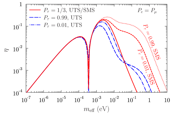
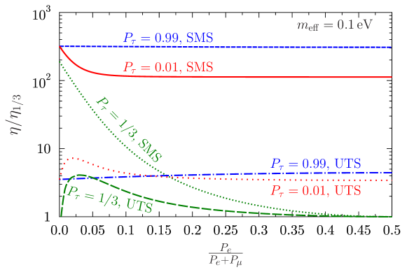
Figure 13: Top panel: the dependence of $\eta$ on the washout parameter $m_{\rm eff}$ for $P_{e}=P_{\mu}$ and different values of $P_{\tau}$. Bottom panel: the dependence of $\eta$ for different flavour configurations $P_{\alpha}$ normalized to $\eta_{1/3}$ that corresponds to the flavour equipartition case $P_{\alpha}=1/3$.

The dependence of the efficiency factor on the flavour projectors $P_{\alpha}$ and on $m_{\rm eff}$ is shown in Fig. 13. The top panel shows the dependence of the efficiency on $m_{\rm eff}$ in the flavour equipartition case and for two other sets of flavour projections. As already mentioned, flavour effects become more relevant when the washouts get stronger. This is confirmed in this picture where it is seen that for the SMS scenario the possible enhancements quickly grow with $m_{\rm eff}$. Note that in SL this dependence is even stronger than in standard leptogenesis. This is due to the fact that the flavoured washout parameters $P_{\alpha}m_{\rm eff}$ also determine the value of $z^{\alpha}_{dec}$ when the lepton asymmetry in the $\alpha$ flavour starts being generated, and since the CP asymmetry has a strong dependence on $z$, different values of $P_{e},\,P_{\mu},\,$ and $P_{\tau}$ imply that the corresponding flavour asymmetries are generated with different values of the CP asymmetry even when, as in the SMS, the fundamental quantity $\bar{\epsilon}$ is flavour independent. In summary, what happens is that the flavour that suffers the weakest washout is also the one for which inverse-decays go out of equilibrium earlier, and thus also the one for which the lepton asymmetry starts being generated when $\bar{\epsilon}\times\Delta_{BF}$ is larger. This realizes a very efficient scheme in which the flavour that is more weakly washed out has effectively the largest CP asymmetry, and this explains qualitatively the origin of the large enhancements that we have found. Furthermore, when $P_{\alpha}m_{\rm eff}\ll m_{*}$ so that the inverse decay of flavour $\alpha$ never reaches equilibrium and the washout of the asymmetry $Y_{\Delta_{\alpha}}$ is negligible, the maximum efficiency is reached.

The bottom panel in Fig. 13 further illustrates how the departure from the equipartition flavour case results in an enhancement of the efficiency, and that particularly large enhancements are possible for the SMS scenario. Note that the top line in the top panel of Fig. 13 labeled $P_{\tau}=0.99$ represents the maximum enhancement that can be obtained in the SMS (relaxing the constraint in Eq. (143) that defines our SMS, larger enhancements are however possible). This is because for $P_{\tau}=0.99$ both the asymmetries $Y_{\Delta_{e}}$ and $Y_{\Delta_{\mu}}$ are generated in the weak washout regime, that is, approximately within the same temperature range, and in the SMS this implies $\epsilon_{e}(T_{e})\approx\epsilon_{\mu}(T_{\mu})$. The related combined efficiency is then simply determined by $(P_{e}+P_{\mu})\,m_{\rm eff}\simeq m_{*}$ and is thus always maximal, independently of the individual values of $P_{e}$ and $P_{\mu}$, as it is apparent from the figure.

We should however spend a word of caution for the reader about interpreting these results in the weak washout regime and, for the SMS, also in the limit of extreme flavour hierarchies ($P_{\alpha}\to 0$). At high temperatures $(z<1)$ the Higgs bosons (higgsinos) develop a sufficiently large thermal mass to decay into sleptons (leptons) and sneutrinos. The new CP asymmetries associated with these decays could be particularly large,[60] and thus sizable lepton flavour asymmetries could be generated at high temperatures. This type of thermal effects are not included in the analysis here described.

Concerning the flavour decoupling limit within the SMS, clearly when $P_{\alpha}\to 0$ no asymmetry can be generated in the flavour $\alpha$. However, in our SMS flavour asymmetries are defined to be independent of the projectors $P$ and thus survive in the $P\to 0$ limit. On physical grounds, one would expect for example that when one decay branching ratio is suppressed, say, as $P<10^{-5}$, the associated CP asymmetry will be at most of ${\cal O}(10^{-7})$ and thus irrelevant for leptogenesis. This means that for extreme flavour hierarchies, the SMS breaks down as a possible physical realization of SL, and thus in what follows we will restrict our considerations to a range of hierarchies $P\ \hbox to0.0pt{\raise 3.0pt\hbox{$>$}\hss}{\lower 3.0pt\hbox{$\sim$}}\ 10^{-3}$.

As a result one finds that for the SMS scenario with hierarchical Yukawa couplings, successful leptogenesis is possible even for $m_{\rm eff}\gg{\cal O}({\rm eV})$. For example, as it is shown in the right panel of Fig. 13, for $P_{e}=P_{\mu}=5\times 10^{-3}$ and $m_{\rm eff}\sim 5$ eV, we obtain $\eta\sim 10^{-3}$, that yields the estimate

$$Y_{\Delta B}^{0}({\rm SMS},P_{e}=P_{\mu}=5\times 10^{-3},m_{\rm eff}=5\,{\rm eV})\sim 10^{-6}\times\overline{\epsilon}\;.$$ (163)

Thus assuming a large, but still acceptable value of $\bar{\epsilon}\sim 10^{-4}$, SL can successfully generate the observed baryon asymmetry for values of $m_{\rm eff}$ that are about two orders of magnitude larger than what is found in the unflavoured standard leptogenesis scenario.

5.6 Natural values of B

We next describe the impact that flavour enhancements can have in relaxing the constraints on the values of $B$ (and $M$). Here we include only the leading CP asymmetry contribution from mixing Eq. (138). From Eqs. (123), (116), and (54), it is easy to derive the maximum value of $B$ for given values of $M$ and $m_{\rm eff}$:

$$B \leq \frac{\Gamma\left(m_{\rm eff},M\right)}{2}\frac{\left|\mbox{Im}A\right|}{M}\frac{y_{\widetilde{N}}\,\eta(m_{\rm eff})}{Y_{\Delta B}^{CMB}}\left[1+\sqrt{1-\left(\frac{M}{\left|\mbox{Im}A\right|}\frac{Y_{\Delta B}^{CMB}}{y_{\widetilde{N}}\,\eta(m_{\rm eff})}\right)^{2}}\right],$$ (164)

where $y_{\widetilde{N}}=\frac{16}{23}Y_{\widetilde{N}}^{eq\,0}$, $\Gamma(m_{\rm eff},M)$ is given in Eq. (22), $\mbox{Im}A=A\sin\phi_{A}$ and $Y_{\Delta B}^{CMB}$ is the observed baryon asymmetry Eq.(6). Consequently we obtain

$$M \leq \frac{\left|\mbox{Im}A\right|y_{\widetilde{N}}\,\eta(m_{\rm eff})}{Y_{B_{obs}}}\;,$$ (165)

$$B \leq \frac{3\sqrt{3}m_{\rm eff}}{32\pi v^{2}}\left(\frac{\left|\mbox{Im}A\right|y_{\widetilde{N}}\,\eta(m_{\rm eff})}{Y_{\Delta B}^{CMB}}\right)^{2}\;,$$ (166)

where $\eta(m_{\rm eff})\equiv\eta(m_{\rm eff},P_{\alpha},Z_{\alpha})$ and all residual dependence of $\eta$ on $M$ has been neglected. As seen in the upper panel of Fig. 13, assuming the SMS and for sufficiently hierarchical $P_{\alpha}$, $\eta(m_{\rm eff})$ decreases first very mildly with $m_{\rm eff}$ and – once all the flavours have reached the strong washout regime– it decreases roughly as $\sim m_{\rm eff}^{-2}$. Thus the product $m_{\rm eff}\times\eta(m_{\rm eff})^{2}$ first grows with $m_{\rm eff}$ till it reaches a maximum and then for sufficiently large $m_{\rm eff}$ it decreases $\sim m_{\rm eff}^{-3}$. Therefore, for a fixed value of the projectors, the upper bound on $B$ does not corresponds simply to the maximum allowed value of $m_{\rm eff}$, but it has a more complicated dependence.

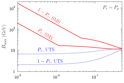
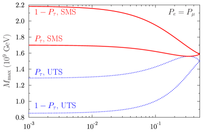
Figure 14: Maximum values of $B$ and $M$ as a function of the flavour projections. To highlight the effects when $P_{\tau}$ is very large or very small, the curves are given as a function of $P_{\tau}$ and of $1-P_{\tau}$.

Fig. 14 shows the maximum values of $B$ and $M$ obtained for both the UTS and SMS cases as a function of the flavour projections. In order to have better resolution when either $P_{\tau}$ or $1-P_{\tau}$ is very small, we plot them both as a function of $P_{\tau}$ or $1-P_{\tau}$. In the figure we set $\mbox{Im}A=1\,$TeV. The figure illustrates that within the UTS, the parameter space for successful leptogenesis is very little modified by departing from the flavour equipartition case (that corresponds to the point where the UTS and SMS curves join). On the contrary, in the SMS case with hierarchical flavour projections $1-P_{\tau}\sim{\rm few}\,\times 10^{-3}$ successful SL is allowed also with $B\sim{\cal O}({\rm TeV})$, that is for quite natural values of the bilinear term. As mentioned above, even for hierarchical projections the maximum allowed values of $B$ and $M$ do not correspond to the maximum allowed value of $m_{\rm eff}$. In particular, for the range of flavour projections shown in the figure we obtain that the maximum values of $B$ and $M$ correspond to $m_{\rm eff}\ \hbox to0.0pt{\raise 3.0pt\hbox{$<$}\hss}{\lower 3.0pt\hbox{$\sim$}}\ 2\,$eV.

5.7 Lepton flavour equilibration and low energy constraints

We finish this section by discussing the impact that the presence of the LFE scatterings discussed in Section 5.3 can have on the enhancement of the efficiency due to flavour effects. We plot in Fig. 15 the dependence of the flavour enhancement of the efficiency as a function of the off-diagonal slepton mass parameter $\widetilde{m}_{od}$. As can be seen in the figure (and as it was expected from the discussion in the previous section) for any given value of $M$, LFE quickly becomes efficient damping completely the lepton flavours enhancements of the efficiency within a very narrow range of values $\widetilde{m}_{od}^{min}\leq\widetilde{m}_{od}\leq\widetilde{m}_{od}^{max}$. The figure corresponds to $\tan\beta=30$ however, as already said, the dependence on $\tan\beta$ arises from $v_{d}=v\cos\beta$ in Eq. (148) and is rather mild. Results from other values of $\tan\beta$ can be easily read from the figure by rescaling $\widetilde{m}^{\beta}_{od}=\widetilde{m}^{\rm fig}_{od}/(30\cos\beta)$.

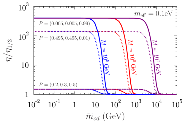
Figure 15: The dependence of the efficiency (normalized to the flavour equipartition case $P_{\alpha}=1/3$) on the off-diagonal soft slepton mass parameter $\widetilde{m}_{od}$, for different values of $M$ and of the flavour projections (see text for details).

Notice that while neglecting LFE the efficiency for a given value of $m_{\rm eff}$ is practically insensitive to the particular value of $M$, this is not the case when the efficiency is evaluated by accounting for LFE effects. In fact, given the different scaling with the temperature of the $\overline{\Gamma}_{\rm LFE}$ and $\overline{\Gamma}_{\rm ID}$ rates, the precise temperature at which leptogenesis occurs is crucial. For example, we see from Fig. 15 that for reasonable values $\widetilde{m}_{od}\ \hbox to0.0pt{\raise 3.0pt\hbox{$<$}\hss}{\lower 3.0pt\hbox{$\sim$}}\ 200\,$GeV and for $M\ \hbox to0.0pt{\raise 3.0pt\hbox{$>$}\hss}{\lower 3.0pt\hbox{$\sim$}}\ 10^{6}\,$GeV, LFE is not effective, and the large enhancements of the efficiency due to flavour effects can survive, while for $M\ \hbox to0.0pt{\raise 3.0pt\hbox{$<$}\hss}{\lower 3.0pt\hbox{$\sim$}}\ 10^{5}\,$GeV all flavour enhancements disappear.

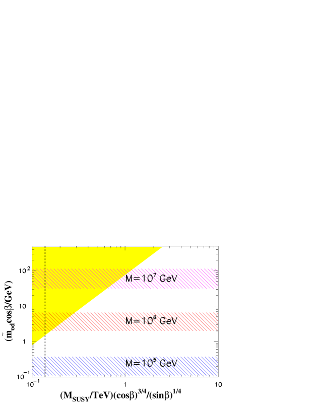
Figure 16: Shaded in yellow: the region of $\widetilde{m}_{od}\cos\beta$ versus $m_{SUSY}(\cos\beta)^{\frac{3}{4}}/(\sin\beta)^{\frac{1}{4}}$ excluded by the present bound $BR(\mu\rightarrow e\gamma)\leq 1.2\times 10^{-11}$. The three bands corresponding to $M=10^{5}\,$GeV, $M=10^{6}\,$GeV and $M=10^{7}\,$GeV show the minimum value of $\widetilde{m}_{od}{\cos\beta}$ for which LFE effects start damping flavour effects. The width of the bands corresponds to $P_{\alpha}m_{\rm eff}$ varying in the range $0.003\,$eV$-10\,$eV, with $P_{\alpha}$ the largest flavour projection. The vertical dashed line corresponds to the value of $m_{SUSY}/(\tan\beta)^{\frac{1}{2}}$ required to explain the discrepancy between the SM prediction and the measured value of $a_{\mu}$, assuming $\tan\beta=1$.[122]

It is interesting notice that the presence of a sizable $\widetilde{m}_{od}$ would induce various LFV decays, like for example $l_{\alpha}\rightarrow l_{\beta}\gamma$ with rate

$$\!\!\!\!\!\!\!\!\!\!\!\!\!\!\!\!\!\!\!\!\!\!\!\!\!\frac{BR(l_{\alpha}\rightarrow l_{\beta}\gamma)}{BR(l_{\alpha}\rightarrow l_{\beta}\nu_{\alpha}\overline{\nu}_{\beta})}\sim\frac{\alpha^{3}}{G_{F}^{2}}\frac{\tan^{2}\beta}{m^{8}_{SUSY}}\widetilde{m}_{od}^{4}$$

$$\simeq 2.9\times 10^{-19}\frac{\sin^{2}\beta}{\cos^{6}\beta}\left(\frac{\rm TeV}{m_{SUSY}}\right)^{8}\left(\cos^{2}\beta\frac{\widetilde{m}_{od}^{2}}{\rm GeV^{2}}\right)^{2},$$ (167)

where $m_{SUSY}$ is a generic SUSY scale for the gauginos and sleptons masses running in the LFV loop. So it is possible to compare the values of $\widetilde{m}_{od}$ for which LFE occurs with the existing bounds imposed from non-observation of such flavour violation in leptonic decays. The result of such comparison in presented in Fig. 16. The yellow shade gives the excluded region of $\widetilde{m}_{od}\,{\cos\beta}$ versus $m_{SUSY}(\cos\beta)^{\frac{3}{4}}/(\sin\beta)^{\frac{1}{4}}$ arising from the present bound BR$(\mu\rightarrow e\gamma)\leq 1.2\times 10^{-11}$, together with the minimum value of $\widetilde{m}_{od}\,{\cos\beta}$ for which LFE effects start damping out flavour enhancements in SL. Three bands are shown respectively for $M=10^{5}\,$GeV, $M=10^{6}\,$GeV and $M=10^{7}\,$GeV. The width of the bands represents the range associated with variations of the effective flavoured decay parameter $P_{\alpha}m_{\rm eff}$ in the range $0.003\,$eV$-10\,$eV, where $P_{\alpha}$ is the largest of the three flavour projections. For illustration we also show in the figure the characteristic SUSY scale that allows to explain the small discrepancy between the SM prediction and the measured value of the muon anomalous magnetic moment, $a_{\mu}$. This values is $m_{SUSY}/(\tan\beta)^{\frac{1}{2}}=141$ GeV,[122] and the vertical dashed line in the picture corresponds to $\tan\beta=1$. As seen in the figure, in this case the off-diagonal slepton masses are bound to be small enough to allow for flavour enhancements in SL for $M$ as low as $10^{6}$ GeV. For larger values of $\tan\beta$, even lower values of $M$ are allowed.

In brief, LFE effects induced by off-diagonal soft slepton masses, when constrained with the bounds imposed from the non-observation of flavour violation in leptonic decays, are ineffective for damping the flavour enhancements.

6 Soft Leptogenesis without Superequilibration: R-genesis

As mentioned in the previous Sections, early works on leptogenesis were carried out from the start within the unflavoured effective theory. Quite likely this happened because the corresponding Lagrangian is much simpler, given that the number of relevant parameters is reduced to a few. The main virtue of subsequent studies on lepton flavour effects was that of recognizing that for $T\lesssim 10^{12}\,$GeV the unflavoured theory breaks down, and the new theory brings in new fundamental parameters, which can give genuinely different answers for the amount of baryon asymmetry that is generated.

In supersymmetric leptogenesis the opposite happened: the effective theory that was generally used assumed fast particle-sparticle equilibration reaction. But this assumption is only appropriate for temperatures much lower than the typical temperatures $T\gg 10^{8}\,$GeV in which leptogenesis can be successful. In fact, only quite recently Ref. Fong:2010qh clarified that in the relevant temperature range, a completely different effective theory holds instead. More specifically, in supersymmetric leptogenesis studies prior to Ref. Fong:2010qh it was always assumed (often implicitly) that lepton-slepton reactions like e.g. $\ell\ell\leftrightarrow\widetilde{\ell}\widetilde{\ell}$ (see Fig. 17) that are induced by soft gaugino masses

$$\mathcal{L}_{\widetilde{\lambda}}=-\frac{1}{2}\left(m_{2}\overline{\widetilde{\lambda}_{2}^{\pm,0}}P_{L}\widetilde{\lambda}_{2}^{\pm,0}+m_{1}\overline{\widetilde{\lambda}_{1}}P_{L}\widetilde{\lambda}_{1}+{\rm h.c.}\right),$$ (168)

as well as higgsino mixing transitions $\widetilde{H}_{u}\leftrightarrow\overline{\widetilde{H}_{d}}$, that are induced by the superpotential term

$$W_{H}=\mu\hat{H}_{u}\hat{H}_{d},$$ (169)

are in thermal equilibrium. This implies that the lepton and slepton chemical potentials equilibrate. However, in general, in supersymmetric leptogenesis superequilibration (SE) between particles and sparticles chemical potentials does not occur. In fact, the rates of interactions induced by SUSY-breaking scale ($\Lambda_{susy}$) parameters, like soft gaugino masses $m_{\widetilde{g}}$ or the higgsino mixing parameter $\mu$, are slower than the Universe expansion rate when

$$\frac{\Lambda_{susy}^{2}}{T}\ \hbox to0.0pt{\raise 3.0pt\hbox{$<$}\hss}{\lower 3.0pt\hbox{$\sim$}}\ 25\;\frac{T^{2}}{M_{pl}}\qquad\Rightarrow\qquad T>T_{\rm SE}\sim 5\cdot 10^{7}\left(\frac{\Lambda_{susy}}{500\,{\rm GeV}}\right)^{2/3}\;{\rm GeV}.$$ (170)

Thus, when this condition is realized, these reactions should be classified as reactions of type (ii) (see Section 3.1) and handled accordingly. Since leptogenesis occurs when the temperature is of the order of the heavy neutrino mass, in terms of $M$ the assumption of SE breaks down when

$$M\ \hbox to0.0pt{\raise 3.0pt\hbox{$>$}\hss}{\lower 3.0pt\hbox{$\sim$}}\ 5\cdot 10^{7}\left(\frac{\Lambda_{susy}}{500\,{\rm GeV}}\right)^{2/3}\,{\rm GeV}.$$ (171)

Following the discussion in Section 3.1, the effective theory appropriate for studying supersymmetric leptogenesis, in which the heavy Majorana masses certainly satisfy the bound Eq. (171), is thus obtained by setting $m_{\widetilde{g}},\,\mu\to 0$.[123, 71] In this limit, the supersymmetric Lagrangian acquires two additional anomalous global symmetries (respectively a $R$-symmetry and a $PQ$-like symmetry) under which, besides the $SU(2)_{L}$ and $SU(3)_{c}$ SM fermions, also the gauginos and higgsinos transform non-trivially. As a consequence, the EW and QCD sphaleron equilibrium conditions are modified with respect to the usual ones: winos, binos and higgsinos are now coupled to the $SU(2)_{L}$ sphalerons, while gluinos get coupled to the QCD sphalerons.[123] Therefore, besides the occurrence of non-superequilibration (NSE) effects, also the pattern of sphaleron induced lepton-flavour mixing is different from what is obtained with a naive supersymmetrization of the SM case.[71] Besides this, a new anomaly-free $R$-symmetry can be defined and the corresponding charge, being exactly conserved, provides a constraint on the particle density asymmetries that is not present in the SM.[71] Nevertheless, in spite of all these modifications, in Ref. Fong:2010qh it was found that eventually the resulting baryon asymmetry would not differ much from what would be obtained with the (incorrect) assumption of SE. Basically, the reason for this is that by dropping the SE assumption and accounting for all the new effects only modifies spectator processes, while the overall amount of CP asymmetry that drives leptogenesis remains the same.

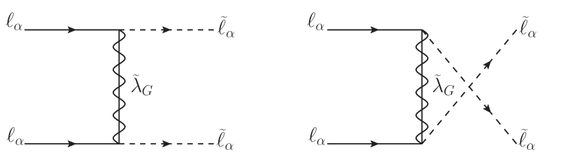
Figure 17: Feynman diagrams for lepton-slepton scatterings induced by soft gaugino masses $m_{\widetilde{g}}$ through the exchange of $SU(2)_{L}$ and $U(1)_{Y}$ gauginos $\widetilde{\lambda}_{G}$. The squared amplitudes of these processes are proportional to $m_{\widetilde{g}}^{2}$ and vanish in the $m_{\widetilde{g}}\to 0$ limit.

In SL however, when $M\ \hbox to0.0pt{\raise 3.0pt\hbox{$>$}\hss}{\lower 3.0pt\hbox{$\sim$}}\ 10^{7}\,$GeV the appropriate NSE effective theory not only implies profound theoretical modifications, but also results in very large quantitative differences. The reason for this is twofold:

(I)  In the NSE regime the leptonic density asymmetries for scalar and fermion evolve independently, and this implies that the corresponding efficiencies $\eta_{s,f}$ are different. When these different ‘weights’ are taken into account, the strong cancellation between the scalar and fermion contributions to the baryon asymmetry, that is characteristic of SL, gets spoiled, and a non-vanishing result is obtained even without the inclusion of thermal corrections.[72]

(II)  While the new symmetries $R$ and $PQ$ that arise in the high temperature effective theory after setting $m_{\widetilde{g}},\mu\to 0$ are anomalous, two anomaly free combinations involving $R$ and $PQ$ can be defined. These combinations, that have been denoted in Ref. Fong:2010bv as ${R_{B}}$ and ${R_{\chi}}$, are conserved in sphaleron transitions, and are only (slowly) violated by RHSN dynamics. Thus their evolutions must be followed by means of two new BE and, since all density asymmetries get mixed by EW sphalerons, these equations couple to the BE that control the evolution of ${B-L}$. What is important is that the sources for ${R_{B}}$ and ${R_{\chi}}$ are respectively the CP-violating asymmetries $\epsilon_{s}$ and $\epsilon_{s}-\epsilon_{f}$, which are not suppressed by any kind of cancellation. Thus the corresponding density asymmetries $Y_{\Delta R_{B}}$ and $Y_{\Delta R_{\chi}}$ remain large during leptogenesis, and act as source terms for the $\Delta_{\alpha}=B/3-L_{\alpha}$ density asymmetries $Y_{\Delta_{\alpha}}$ that are thus driven to comparably large values.

As regards the final values of ${R_{B}}$ and ${R_{\chi}}$ at the end of leptogenesis, they are instead irrelevant for the computation of the baryon asymmetry since, well before the temperature when the EW sphalerons are switched off, soft SUSY-breaking effects attain in-equilibrium rates, implying that $R$ and $PQ$ cease to be good symmetries also at the perturbative level implying that $Y_{\Delta R_{B}},\,Y_{\Delta R_{\chi}}\to 0$. The baryon asymmetry is then determined only by the amount of $B-L$ asymmetry at freeze-out of the EW sphalerons according to the usual relation $B=\frac{8}{23}\,(B-L)$.

6.1 Anomalous and non-anomalous symmetries above $T_{\rm SE}$

As discussed above, when the temperature of the thermal bath satisfies the condition Eq. (170) the appropriate effective supersymmetric Lagrangian is obtained by setting $m_{\widetilde{g}},\mu\to 0$, which results in the two new $U(1)$ symmetries $R$ and $PQ$.[123]

$B$, $L$, $PQ$ and $R$ charges for the particle supermultiplets. The labels in the top row refer to the supermultiplets L-handed fermion components. The $R$ charges for bosons are determined by $R(b)=R(f)+1$.  $\tilde{g}\$  $Q\$  $u^{c}\$  $d^{c}\$  $\ell\$  $e^{c}\$  $\tilde{H}_{d}\phantom{\Big{|}}$  $\tilde{H}_{u}\$  $N^{c}\$ $B\phantom{\Big{|}}$ $0$ $\frac{1}{3}$ $-\frac{1}{3}$ $-\frac{1}{3}$ $0$ $0$ $0$ $0$ 0 $L\phantom{\Big{|}}$ $0$ $0$ $0$ $0$ $1$ $-1$ $0$ $0$ 0 $PQ\phantom{\Big{|}}$ $0$ $0$ $-2$ $1$ $-1$ $2$ $-1$ $2$ 0 $R$ $\phantom{\!\!\!\!\Big{|}}f$ $1$ $-1$ $-3$ $1$ $-1$ $1$ $-1$ $3$ $-1$ $\phantom{\!\!\!\!\Big{|}}b$ $2$ $0$ $-2$ $2$ $0$ $2$ $0$ $4$ 0

The charges of the various states under these symmetries, together with the values of the other two global symmetries $B$ and $L$ are given in Table 6.1. Note that to facilitate the evaluation of the anomalies in the table we list the charges of the L-handed chiral multiplets, and in particular those of $u^{c},\,d^{c},\,e^{c}$ that are opposite with respect to the charges of the R-handed states $u,\,d,\,e$ whose chemical potentials will enter the chemical equilibrium equations below.

Like $L$, also $R$ and $PQ$ are not symmetries of the seesaw superpotential terms $M\hat{N}^{c}\hat{N}^{c}+\lambda\hat{N}^{c}\hat{\ell}\hat{H}_{u}$, since it is not possible to find any charge assignment that would leave both terms invariant. In Table 6.1 the charges of the heavy $N^{c}$ supermultiplets have been fixes so that RHSN do not carry any charge. This has the advantage of ensuring that all the RHSN bilinear terms, corresponding to the mass parameters $M,\,\widetilde{M},\,B$, are invariant, and thus RHSN mixing does not break any internal symmetry. However, since $R(\hat{N}^{c}\hat{N}^{c})=0$, it follows that the mass term for the heavy RHN breaks $R$ by two units.

All the four global symmetries $B$, $L$, $PQ$ and $R$ have mixed gauge anomalies with $SU(2)_{L}$, and $R$ and $PQ$ have also mixed gauge anomalies with $SU(3)_{c}$. Two linear combinations of $R$ and $PQ$, having respectively only $SU(2)_{L}$ and $SU(3)_{c}$ mixed anomalies, have been identified in Ref. Ibanez:1992aj. They are:

$$R_{2} = R-2\,PQ$$ (172)

$$R_{3} = R-3\,PQ\,.$$ (173)

The values of $R_{2,3}$ for the different states are given in Table 6.1. The authors of Ref. Ibanez:1992aj have also constructed the effective multi-fermions operators generated by the mixed anomalies:

$$\tilde{O}_{EW} = \Pi_{\alpha}\left(QQQ\ell_{\alpha}\right)\;\tilde{H}_{u}\tilde{H}_{d}\;\tilde{W}^{4}\,,$$ (174)

$$\tilde{O}_{QCD} = \Pi_{i}\left(QQu^{c}d^{c}\right)_{i}\;\tilde{g}^{6}\,.$$ (175)

Given that the three charges $R_{2}$, $B$ and $L$ all have mixed $SU(2)_{L}$ anomalies, two anomaly free combinations can be defined. The most convenient are $B-L$ and[72]

$${R_{B}}=\frac{2}{3}B+R_{2},$$ (176)

whose values are also given in Table 6.1. The fact that $R_{B}$ does not contain any $B-L$ fragment, ensures that it will not enter in the final computation of the baryon asymmetry, and the fact that it is independent of $L$ renders easier writing the BE for its evolution. The values of $R_{B}$ in Table 6.1 imply that the superpotential term $N^{c}\,\ell H_{u}$ has charge $R_{B}=2$ and thus is invariant. It follows that RHSN decays into fermions conserve $R_{B}$. In contrast, the soft $A$ term in Eq. (12) responsible for RHSN decays into scalars violates $R_{B}$ by 2 units, and more precisely for $\widetilde{N}_{\pm}\to H_{u}\tilde{\ell}$ we have $\Delta R_{B}=+2$, while for $\widetilde{N}_{\pm}\to H_{u}^{*}\tilde{\ell}^{*}$ we have $\Delta R_{B}=-2$. As regards the heavy neutrinos, their mass term violates $R_{B}$ by two units. Note that this is precisely like the case when one chooses to assign a lepton number $-1$ to the singlet neutrinos $N$. Accordingly, the decays of the heavy Majorana neutrino violate $R_{B}$ by one unit: for $N\to\ell H_{u},\,\tilde{\ell}\tilde{H}_{u}$ we have $\Delta R_{B}=+1$ while for the CP conjugate final states $\Delta R_{B}=-1$. All $R_{B}$ violating reactions have, by assumption, rates that are comparable to the Universe expansion rate, and then a specific BE is needed to track the evolution of $Y_{\Delta R_{B}}$.

Charges for the fermionic and bosonic components of the SUSY multiplets under the $R$-symmetries defined in Eqs.(172), (173) and (176). Supermultiplets are labeled in the top row by their L-handed fermion component.  $\tilde{g}\$  $Q\$  $u^{c}\$  $d^{c}\$  $\ell\$  $e^{c}\$  $\tilde{H}_{d}\phantom{\Big{|}}$  $\tilde{H}_{u}\$  $N^{c}\$ $R_{2}$ $\phantom{\!\!\!\!\Big{|}}f$ $1$ $-1$ $1$ $-1$ $1$ $-3$ $1$ $-1$ $-1$ $\phantom{\!\!\!\!\Big{|}}b$ $2$ $0$ $2$ $0$ $2$ $-2$ $2$ $0$ 0 $R_{3}$ $\phantom{\!\!\!\!\Big{|}}f$ $1$ $-1$ $3$ $-2$ $2$ $-5$ $2$ $-3$ $-1$ $\phantom{\!\!\!\!\Big{|}}b$ $2$ $0$ $4$ $-1$ $3$ $-4$ $3$ $-2$ 0 $R_{B}$ $\phantom{\!\!\!\!\Big{|}}f$ $1$ $-\frac{7}{9}$ $\frac{7}{9}$ $-\frac{11}{9}$ $1$ $-3$ $1$ $-1$ $-1$ $\phantom{\!\!\!\!\Big{|}}b$ $2$ $\frac{2}{9}$ $\frac{16}{9}$ $-\frac{2}{9}$ $2$ $-2$ $2$ $0$ 0

At temperatures satisfying condition Eq. (170) there is at least one other anomalous global symmetry, that in Ref. Fong:2010bv has been denoted by $\chi$. It corresponds to $U(1)$ phase rotations of the $u^{c}$ chiral multiplet that, for its fermionic component, can be readily identified with chiral symmetry for the right-handed up-quark. In fact, above $T\sim 2\times 10^{6}\,$GeV, reactions mediated by $h_{u}$ do not occur and the condition $h_{u}\to 0$ must be imposed, resulting in a new anomalous ‘chiral’ symmetry. In the $SU(3)_{c}$ sector we then have two anomalous symmetries $R_{3}$ and $\chi$, and one anomaly free combination can be constructed. Assigning to the $L$-handed $u^{c}_{L}$ supermultiplet a chiral charge $\chi=-1$ this combination has the form[71]

$$R_{\chi}=\raise 2.0pt\hbox{$\chi$}_{u^{c}_{L}}+\kappa_{u^{c}_{L}}\,R_{3},$$ (177)

where $\kappa_{u^{c}_{L}}=1/3$. When the additional condition $h_{d}\to 0$ is imposed, a chiral symmetry arises also for the $d^{c}$ supermultiplet. A second anomaly free $R_{\chi}$ symmetry can then be defined in a way completely analogous to Eq. (177), with $\kappa_{d^{c}_{L}}=\kappa_{u^{c}_{L}}=1/3$.[71] As regards perturbative violation of $R_{\chi}$, this charge inherits the same violation $R_{3}$ suffers. The soft $A$ term in Eq. (12) violates $R_{3}$ by one unit, and so do RHSN decays into scalars. Moreover, since $N^{c}\,\ell H_{u}$ has an overall charge $R_{3}=1$, a violation by one unit occurs also for RHSN decays into fermions. Correspondingly, we have $\Delta R_{3}=+1$ for the decays $\tilde{N},\,\tilde{N}^{*}\to H_{u}\tilde{\ell},\;\overline{\widetilde{H}}_{u}\overline{\ell}$ and $\Delta R_{3}=-1$ for $\tilde{N},\,\tilde{N}^{*}\to\widetilde{H}_{u}\ell,\;H_{u}^{*}\tilde{\ell}^{*}$. Of course, similarly to $R_{B}$, also the evolution of $R_{\chi}$ needs to be tracked by means of one BE.

6.2 Chemical equilibrium conditions and conservation laws

Because of the network of fast particle reactions occurring in the thermal bath, asymmetries generated in RHSN decays spread around among the various particle species, and this can affect directly or indirectly leptogenesis processes. In principle there is one asymmetry for each particle degree of freedom. There are however several conditions and constraints that reduce the number of independent asymmetries to a few.

• Constraints imposed by reactions whose rates are much faster than the Universe expansion have to be formulated in terms of chemical equilibrium conditions for the chemical potentials of incoming $\mu_{I}$ and final state particles $\mu_{F}$:

  $$\sum_{I}\mu_{I}=\sum_{F}\mu_{F}.$$ (178)

• Conservation laws that arise when all the reactions that violate some specific charge are much slower than the the Universe expansion have to be formulated in terms of particle number densities $\Delta n=n-\bar{n}$ and, for a generic charge $Q$, read:

  $$Q=\sum_{i}Q_{i}\Delta n_{i}={\rm const},$$ (179)

  where $Q_{i}$ is the charge of the $i$-particle species. We will always assume as initial conditions for leptogenesis that all particle asymmetries vanish, and thus we will put the constant value of Eq. (179) equals to zero.

• Reactions with rates comparable with the Universe expansion have to be treated by means of appropriate dynamical equations. In this case, in order to reabsorb the dilution effects due to the Universe expansion, it is convenient to introduce as basic variables the number densities of particles normalized to the entropy density $s$ so we define the density asymmetries per degree of freedom $g_{i}$:

  $$Y_{\Delta_{i}}=\frac{1}{g_{i}}\frac{\Delta n_{i}}{s}\,.$$ (180)

Clearly, $\mu_{i}$, $\Delta n_{i}$ and $Y_{\Delta_{i}}$ are all related to particle asymmetries. In particular, the number density asymmetry of a particle for which a chemical potential can be defined is directly related with this chemical potential. For both bosons ($b$) and fermions ($f$) this relation acquires a particularly simple form in the relativistic limit $m_{b,f}\ll T$, and at first order in $\mu_{b,f}/T\ll 1$:

$$\Delta n_{b}=\frac{g_{b}}{3}T^{2}\mu_{b},\qquad\quad\Delta n_{f}=\frac{g_{f}}{6}T^{2}\mu_{f}\,.$$ (181)

Eventually, to solve for the large set of conditions in a closed form one needs to use a single set of variables. Here we will take this to be the set $\left\{Y_{\Delta_{i}}\right\}$, leaving understood that the solutions to the constraining conditions are obtained after expressing $\mu_{i}$ and $\Delta n_{i}$ in terms of this set through Eq. (181) and Eq. (180).

6.2.1 General constraints

We first list in items 1, 2 and 3 below the conditions that hold in the whole temperature range $M_{W}\ll T\ \hbox to0.0pt{\raise 3.0pt\hbox{$<$}\hss}{\lower 3.0pt\hbox{$\sim$}}\ 10^{14}\,$GeV. Conversely, some of the Yukawa coupling conditions given in items 4 and 5 will have to be dropped as the temperature is increased and the corresponding reactions go out of equilibrium. For simplicity of notations, in the following we denote the chemical potentials with the same notation that labels the corresponding field: $\phi\equiv\mu_{\phi}$.

1. At scales much higher than $M_{W}$, gauge fields have vanishing chemical potential $W=B=g=0$.[88] This also implies that all the particles belonging to the same $SU(2)_{L}$ or $SU(3)_{c}$ multiplets have the same chemical potential. For example $\phi(I_{3}=+\frac{1}{2})=\phi(I_{3}=-\frac{1}{2})$ for a field $\phi$ that is a doublet of weak isospin $\vec{I}$, and similarly for color.

2. Denoting by $\tilde{W}_{R}$, $\tilde{B}_{R}$ and $\tilde{g}_{R}$ the right-handed winos, binos and gluinos chemical potentials, and by $\ell,\,Q$ ($\tilde{\ell},\,\tilde{Q}$) the chemical potentials of the (s)lepton and (s)quarks left-handed doublets, the following reactions: $\tilde{Q}+\tilde{g}_{R}\to Q$, $\tilde{Q}+\tilde{W}_{R}\to Q$, $\tilde{\ell}+\tilde{W}_{R}\to\ell$, $\tilde{\ell}+\tilde{B}_{R}\to\ell$, imply that all gauginos have the same chemical potential:

   $$-\tilde{g}=Q-\tilde{Q}=-\tilde{W}=\ell-\tilde{\ell}=-\tilde{B},$$ (182)

   where $\tilde{W}$, $\tilde{B}$ and $\tilde{g}$ denote the chemical potentials of left-handed gauginos. It follows that the chemical potentials of the SM particles are related to those of their respective superpartners as

   $$\tilde{Q},\tilde{\ell} = Q,\ell+\tilde{g}$$ (183)

   $$H_{u,d} = \tilde{H}_{u,d}+\tilde{g}$$ (184)

   $$\tilde{u},\tilde{d},\tilde{e} = u,d,e-\tilde{g}.$$ (185)

   The last relation, in which $u,d,e\equiv u_{R},d_{R},e_{R}$ denote the $R$-handed $SU(2)_{L}$ singlets, follows e.g. from $\tilde{u}^{c}_{L}=u^{c}_{L}+\tilde{g}$ for the corresponding $L$-handed fields, together with $u^{c}_{L}=-u_{R}$, and from the analogous relation for the $SU(2)_{L}$ singlet squarks.

Eqs. (183)–(185) together with the vanishing of the chemical potentials of the gauge fields and the equality of the chemical potentials for all the gauginos, imply that we are left with 18 chemical potentials (or number density asymmetries) that we choose to be the ones of the fermionic states. They are 15 for the SM quarks and leptons, 2 for the up-type and down-type higgsinos, and 1 for the gauginos. These 18 quantities are further constrained by additional conditions.

1. Before EW symmetry breaking hypercharge is an exactly conserved quantity, and we can assume a vanishing total hypercharge for the Universe:

   $${y}_{\,\rm tot}=\sum_{b}\Delta n_{b}\,y_{b}+\sum_{f}\Delta n_{f}\,y_{f}=0,$$ (186)

   where $y_{b,f}$ denotes the hypercharge of the $b$-bosons or $f$-fermions. It is useful to rewrite explicitly this condition in terms of the rescaled density asymmetries per degree of freedom $\left\{Y_{\Delta_{i}}\right\}$ defined in Eq. (180):

   $$\sum_{i}\left(Y_{\Delta Q_{i}}+2Y_{\Delta u_{i}}-Y_{\Delta d_{i}}\right)-\sum_{\alpha}\left(Y_{\Delta\ell_{\alpha}}+Y_{\Delta e_{\alpha}}\right)+Y_{\Delta\tilde{H}_{u}}-Y_{\Delta\tilde{H}_{d}}=0.$$ (187)

2. When the reactions mediated by the lepton Yukawa couplings are faster than the Universe expansion rate, the following chemical equilibrium conditions are enforced:

   $$\ell_{\alpha}-e_{\alpha}+\tilde{H}_{d}+\tilde{g}=0,\qquad(\alpha=e,\,\mu,\,\tau).$$ (188)

   For $\alpha=e$ the corresponding Yukawa condition holds only as long as

   $$T\ \hbox to0.0pt{\raise 3.0pt\hbox{$<$}\hss}{\lower 3.0pt\hbox{$\sim$}}\ 10^{5}(1+\tan^{2}\beta)\,{\rm GeV,}$$

   when Yukawa reactions between the first generation left-handed $SU(2)_{L}$ lepton doublet $\ell_{e}$ and the right-handed singlet $e$ are faster than the expansion.[124, 117] Note also that, as discussed in Section 5.7, if the temperature is not too low lepton flavour equilibration induced by off-diagonal slepton soft masses will not occur. We assume that this is the case, and thus we take the three $\ell_{\alpha}$ to be independent quantities.

3. Reactions mediated by the quark Yukawa couplings enforce the following six chemical equilibrium conditions:

   $$Q_{i}-u_{i}+\tilde{H}_{u}+\tilde{g} = 0,\qquad(u_{i}=u,\,c,\,t),$$ (189)

   $$Q_{i}-d_{i}+\tilde{H}_{d}+\tilde{g} = 0,\qquad(d_{i}=d,\,s,\,b)\,.$$ (190)

   The up-quark Yukawa coupling maintains chemical equilibrium between the left- and right-handed up-type quarks up to $T\sim 2\cdot 10^{6}\,$GeV. Note that when the Yukawa reactions of at least two families of quarks are in equilibrium, the mass basis is fixed for all the quarks and squarks. Intergeneration mixing then implies that family-changing charged-current transitions are also in equilibrium: $b_{L}\to c_{L}$ and $t_{L}\to s_{L}$ imply $Q_{2}=Q_{3}$; $s_{L}\to u_{L}$ and $c_{L}\to d_{L}$ imply $Q_{1}=Q_{2}$. Thus, up to temperatures $T\ \hbox to0.0pt{\raise 3.0pt\hbox{$<$}\hss}{\lower 3.0pt\hbox{$\sim$}}\ 10^{11}\,$GeV, that are of the order of the equilibration temperature for the charm Yukawa coupling, the three quark doublets have the same chemical potential:

   $$Q\equiv Q_{3}=Q_{2}=Q_{1}.$$ (191)

   At higher temperatures, when only the third family is in equilibrium, we have instead $Q\equiv Q_{3}=Q_{2}\neq Q_{1}$. Above $T\sim 10^{13}$ when (for moderate values of $\tan\beta$) also the $\tau$ and $b$-quark $SU(2)_{L}$ singlets decouple from their Yukawa reactions, all intergeneration mixing becomes negligible and $Q_{3}\neq Q_{2}\neq Q_{1}$.

6.2.2 Above the superequilibration temperature

We now discuss the condition specific for ranges of temperatures satisfying Eq. (170), for which the chemical potentials of particle $\phi$ and of its superpartner $\widetilde{\phi}$ are not equal (NSE) but are related through a (non-vanishing) gaugino chemical potential $\widetilde{g}$, as in Eqs. (183)–(185). For definiteness, we fix the relevant temperature around $T\sim 10^{8}\,$GeV, and to emphasize that this condition applies only to the NSE regime we put the subscript ‘NSE’ on the numbering.

1. Fast reactions induced by the generalized QCD and EW sphaleron multi-fermion operators Eq. (174) and Eq. (175) imply[123]

   $$3\sum_{i}Q_{i}+\sum_{\alpha}\ell_{\alpha}+\tilde{H}_{u}+\tilde{H}_{d}+4\,\tilde{g}=0,$$ (192)

   $$2\sum_{i}Q_{i}-\sum_{i}\left(u_{i}+d_{i}\right)+6\,\tilde{g}=0.$$ (193)

At $T\sim 10^{8}\,$GeV, Yukawa equilibrium for the $u$ quark is never realized. For $\alpha=e$ and for the $d$-quark Yukawa, equilibrium holds as long as $T\ \hbox to0.0pt{\raise 3.0pt\hbox{$<$}\hss}{\lower 3.0pt\hbox{$\sim$}}\ 10^{5}(1+\tan^{2}\beta)\,{\rm GeV}$[124, 117] and $T\ \hbox to0.0pt{\raise 3.0pt\hbox{$<$}\hss}{\lower 3.0pt\hbox{$\sim$}}\ 4\cdot 10^{6}(1+\tan^{2}\beta)\,{\rm GeV}$ respectively. Then, for $T\sim 10^{8}\,$GeV both condition hold only if $\tan\beta\ \hbox to0.0pt{\raise 3.0pt\hbox{$>$}\hss}{\lower 3.0pt\hbox{$\sim$}}\ 35$, while they both do not hold if $\tan\beta\ \hbox to0.0pt{\raise 3.0pt\hbox{$<$}\hss}{\lower 3.0pt\hbox{$\sim$}}\ 5$. As we will discuss below, in the latter case the Yukawa equilibrium conditions get replaced by other two conditions, and thus the overall number of constraints does not change. Later in Section 6.2.3 we will present results for the large and small $\tan\beta$ cases, and since they do not differ much, we omit the corresponding results for the intermediate case $5\ \hbox to0.0pt{\raise 3.0pt\hbox{$<$}\hss}{\lower 3.0pt\hbox{$\sim$}}\ \tan\beta\ \hbox to0.0pt{\raise 3.0pt\hbox{$<$}\hss}{\lower 3.0pt\hbox{$\sim$}}\ 35$.

Counting the number of additional conditions listed in items 3–5 and 6_NSE, we have 1 from global hypercharge neutrality, 8 from Yukawa equilibrium plus 2 from intergeneration quark mixing, and 2 from the EW and QCD sphaleron equilibrium. This adds to a total of 13 constraints for the initial 18 variables, meaning that 5 quantities must be determined from dynamical evolution equations. These quantities can be chosen, for example, as the density asymmetries of the three fermionic lepton flavours $Y_{\Delta\ell_{\alpha}}$, of the up-type higgsinos $Y_{\Delta\tilde{H}_{u}}$ and of the gauginos $Y_{\Delta\tilde{g}}$, given that the last one allows to relate $Y_{\Delta\ell_{\alpha}}$ and $Y_{\Delta\tilde{H}_{u}}$ to the densities asymmetries of the corresponding superpartners. This choice would be a natural one since these are the density asymmetries that ‘weight’ the various interactions entering the BE for SL. However, the EW and QCD sphaleron reactions Eq. (174) and Eq. (175) imply fast changes of these asymmetries. A much more convenient choice will be to use appropriate linear combinations of the various asymmetries corresponding to anomaly free and quasi-conserved charges, where with ‘quasi-conserved’ we refer to charges that are not conserved only by the ‘slow’ RHSN-related reactions. These quantities can be identified with the three flavoured charges $\Delta_{\alpha}$ and with the two charges $R_{B}$ and $R_{\chi}$ discussed in the previous section. In terms of the rescaled density asymmetries (asymmetry abundances) per degree of freedom they read:

$$Y_{\Delta_{\alpha}} = 6\,Y_{\Delta Q}+\sum_{i}\left(Y_{\Delta u_{i}}+Y_{\Delta d_{i}}\right)-3\,(2Y_{\Delta\ell_{\alpha}}+Y_{\Delta e_{\alpha}})-2\,Y_{\Delta\tilde{g}}\,,$$ (194)

$$Y_{\Delta R_{B}} = -6Y_{\Delta Q}-\sum_{i}\left(13\,Y_{\Delta u_{i}}-5\,Y_{\Delta d_{i}}\right)$$ (195)

$$+\sum_{\alpha}\left(10\,Y_{\Delta\ell_{\alpha}}+7\,Y_{\Delta e_{\alpha}}\right)+68\,Y_{\Delta\tilde{g}}+10\,Y_{\Delta\tilde{H}_{d}}-2\,Y_{\Delta\tilde{H}_{u}},$$

and

$$Y_{\Delta R_{\chi}} = 3\,\sum_{i}\left(3\,Y_{\Delta u_{i}}-2\,Y_{\Delta\tilde{g}}\right)+\frac{1}{3}\,Y_{\Delta R_{3}},$$ (196)

where, in this last expression,

$$Y_{\Delta R_{3}} = -18Y_{\Delta Q}-3\,\sum_{i}\left(11\,Y_{\Delta u_{i}}-4\,Y_{\Delta d_{i}}\right)$$ (197)

$$+\sum_{\alpha}\left(16\,Y_{\Delta\ell_{\alpha}}+13\,Y_{\Delta e_{\alpha}}\right)+82\,Y_{\Delta\tilde{g}}+16\,Y_{\Delta\tilde{H}_{d}}-14\,Y_{\Delta\tilde{H}_{u}}.$$

The asymmetry abundances of the five charges in Eqs. (194)-(196) define the basis $Y_{\Delta_{a}}=\left\{Y_{\Delta_{\alpha}},Y_{\Delta R_{B}},Y_{\Delta R_{\chi}}\right\}$ in terms of which the five fermionic asymmetry abundances $Y_{\Delta\psi_{a}}=\{Y_{\Delta\ell_{\alpha}},\,Y_{\Delta\tilde{g}},\,Y_{\Delta\tilde{H}_{u}}\}$, that are the relevant ones for the SL processes, have to be expressed. We will do this by introducing a $5\times 5$ $A$-matrix defined according to:

$$Y_{\Delta\psi_{a}}=A_{ab}\,Y_{\Delta_{b}}\,,$$ (198)

where the numerical values of $A_{ab}$ are obtained from Eqs. (194)-(196) subjected to the constraining conditions listed in items 3–5 and 6_NSE. Let us note at this point that the $3\times 5$ submatrix $A_{\ell_{\alpha}b}$ for the lepton asymmetry abundances represents the generalization of the $A$ matrix introduced in Ref. Barbieri:2000, $A_{\tilde{H}_{u}b}$ generalizes the Higgs $C$-vector first introduced in Ref. Nardi:2006a, and $A_{\tilde{g}b}$ generalizes the $C$-vector for the gauginos first introduced in Ref. Fong:2010qh. As regards the asymmetry abundances for the bosonic partners of $\ell_{\alpha}$ and of $\widetilde{H}_{u}$, they are simply given by: $A_{\widetilde{\ell}_{\alpha}\,b}=2\left(A_{\ell_{\alpha}\,b}+A_{\widetilde{g}b}\right)$ and $A_{H_{u}\,b}=2\left(A_{\widetilde{H}_{u}}+A_{\widetilde{g}\,b}\right)$.

6.2.3 Additional conditions from Yukawa reactions

1. Case I: Electron and down-quark Yukawa reactions in equilibrium.
   If the down-type Higgs VEV is relatively small $v_{d}\ll v$, the values of the electron and down-quark masses are obtained for correspondingly large values of the $h_{d}$ and $h_{e}$ Yukawa couplings. For $v_{u}/v_{d}=\tan\beta\ \hbox to0.0pt{\raise 3.0pt\hbox{$>$}\hss}{\lower 3.0pt\hbox{$\sim$}}\ 35$ we have a regime in which at $T\sim 10^{8}\,$GeV, that is well above the NSE threshold Eq. (170), both $h_{d}$ and $h_{e}$ related reactions are in equilibrium. Since $u$-quark Yukawa reactions are never in equilibrium, in this case, only eight Yukawa conditions in Eqs. (188)-(190) hold. Solving for the density asymmetries $Y_{\Delta\psi_{a}}=\{Y_{\Delta\ell_{\alpha}},\,Y_{\Delta\tilde{g}},\,Y_{\Delta\tilde{H}_{u}}\}$ in terms of the charge-asymmetries $Y_{\Delta_{a}}=\left\{Y_{\Delta_{\alpha}},Y_{\Delta R_{B}},Y_{\Delta R_{\chi}}\right\}$ subject to the constraints in items 3 to 5 and 6_NSE, yields

   $$A=\frac{1}{9\times 827466}\left(\begin{array}[]{rrrrr}-788776&38690&38690&-56295&41931\\ 38690&-788776&38690&-56295&41931\\ 38690&38690&-788776&-56295&41931\\ 41913&41913&41913&124281&12798\\ -102411&-102411&-102411&108108&-335907\end{array}\right).$$ (199)

2. Case II: Electron and down-quark Yukawa reactions out of equilibrium
   If $v_{d}$ is not much smaller than $v_{u}$, resulting in $\tan\beta\ \hbox to0.0pt{\raise 3.0pt\hbox{$<$}\hss}{\lower 3.0pt\hbox{$\sim$}}\ 5$, then both $h_{e}$ and $h_{d}$ are sufficiently small that at $T\sim 10^{8}\,$GeV the related Yukawa reactions do not occur. In this case we have to set $h_{d},\,h_{e}\to 0$ and the corresponding two Yukawa equilibrium conditions in Eqs. (188)-(190) do not hold (on top of $u$-quark Yukawa reactions which are never in equilibrium). However, two conservation laws replace these conditions. $h_{e}\to 0$ implies that we gain a ‘chiral’ symmetry for the right-handed fermion and scalar electrons, ensuring that the total number density asymmetry $\Delta n_{e}+\Delta n_{\tilde{e}}$ is conserved. As usual, we assume that the constant value of this quantity vanishes, which in terms of the rescaled density asymmetries per degree of freedom implies:

   $$Y_{\Delta e}-\frac{2}{3}\,Y_{\Delta\tilde{g}}=0\,.$$ (200)

   For the right-handed down quark we could define an anomaly-free charge completely equivalent to $Y_{\Delta R_{\chi}}$ in Eq. (196) but, given that in this regime all the dynamical equations are symmetric under the exchange $u\leftrightarrow d$, it is equivalent, and much more simple, to impose the condition

   $$Y_{\Delta d}=Y_{\Delta u}\,.$$ (201)

   The net result is that, with respect to the previous case, the total number of constraints is not changed, and again five quantities suffice to express the rescaled density asymmetries for all the fields. For the $5\times 5$ $A$ matrix defined in Eq. (198) we obtain:

   $$A=\frac{1}{9\times 162332}\left(\begin{array}[]{rrrrr}-210531&21573&21573&-12414&12483\\ 8676&-165529&-3197&-17958&29709\\ 8678&-3197&-165529&-17958&29709\\ 7497&7299&7299&23634&4833\\ -11322&-18477&-18477&23940&-74385\end{array}\right).$$ (202)

6.3 Boltzmann equations for R-genesis

In order to render clear the role played by the new charges $\Delta R_{B}$ and $\Delta R_{\chi}$ and by NSE effects, in this section we introduce a simplified set of BE including only decays and inverse decays of RHN and RHSN. In this approximation the evolutions of the number density of the heavy states normalized to the entropy density $s$ is obtained from Eqs. (110) and (111) by retaining only the two reactions rates $\gamma_{\widetilde{N}}$ and $\gamma_{{N}}$. In writing down the evolution equations for the five charges $Y_{\Delta_{\alpha}},Y_{\Delta R_{B}},Y_{\Delta R_{\chi}}$ it is convenient to introduce a special notation for the scalar and fermionic asymmetry abundances (per degree of freedom) normalized to the respective equilibrium abundances $Y^{eq}_{s}=2Y^{eq}_{f}=\frac{15}{4\pi^{2}g_{*}}$:

$${\cal Y}_{\Delta s,\Delta f}\equiv\frac{Y_{\Delta s,\Delta f}}{Y^{eq}_{s,f}}.$$ (203)

Using Eqs. (180) and (181) together with Eqs. (183) and (184) it is then easy to verify that

$${\cal Y}_{\Delta\tilde{\ell},\Delta H_{u}}={\cal Y}_{\Delta\ell,\Delta\tilde{H}_{u}}+{\cal Y}_{\Delta\tilde{g}}\,.$$ (204)

Retaining only decays and inverse decays, the BE for the flavour density asymmetries read:

$$\dot{Y}_{\Delta_{\alpha}} = -\epsilon^{f}_{\alpha}\left(z\right)\left(\frac{Y_{\widetilde{N}}}{Y_{\widetilde{N}_{+}}^{eq}}-2\right)\frac{\gamma_{\widetilde{N}}}{2}+\left({\cal Y}_{\Delta\ell_{\alpha}}+{\cal Y}_{\Delta\widetilde{H}_{u}}\right)\frac{\gamma_{\widetilde{N}}^{f,\alpha}}{2}+\Big{(}{\cal Y}_{\Delta\ell_{\alpha}}+{\cal Y}_{\Delta H_{u}}\Big{)}\frac{\gamma_{N}^{\alpha}}{4}$$ (205)

$$-\epsilon^{s}_{\alpha}\left(z\right)\left(\frac{Y_{\widetilde{N}}}{Y_{\widetilde{N}_{+}}^{eq}}-2\right)\frac{\gamma_{\widetilde{N}}}{2}+\left({\cal Y}_{\Delta\widetilde{\ell}_{\alpha}}+{\cal Y}_{\Delta H_{u}}\right)\frac{\gamma_{\widetilde{N}}^{s,\alpha}}{2}+\left({\cal Y}_{\Delta\widetilde{\ell}_{\alpha}}+{\cal Y}_{\Delta\widetilde{H}_{u}}\right)\frac{\gamma_{N}^{\alpha}}{4},$$

where $\gamma_{\widetilde{N}}^{s(f),\alpha}$ denotes the rate of RHSN decays into scalars (fermions) of flavour $\alpha$, while quantities without a flavour index are understood to be summed over all flavours. To an excellent approximation we have $\gamma_{\widetilde{N}}^{s,\alpha}=\gamma_{\widetilde{N}}^{f,\alpha}$, and furthermore the density asymmetries of the scalars can be expressed in terms of the ones of the fermions by means of Eq. (204). This yields:

$$\dot{Y}_{\Delta_{\alpha}}\! = \!-\epsilon_{\alpha}\left(z\right)\left(\frac{Y_{\widetilde{N}}}{Y_{\widetilde{N}_{+}}^{eq}}-2\right)\frac{\gamma_{\widetilde{N}}}{2}+\left({\cal Y}_{\Delta\ell_{\alpha}}+{\cal Y}_{\Delta\widetilde{H}_{u}}+{\cal Y}_{\Delta\widetilde{g}}\right)\!\!\frac{\gamma_{N}^{\alpha}+\gamma_{\widetilde{N}}^{\alpha}}{2},$$ (206)

$$\dot{Y}_{\Delta R_{B}}\! = \!\epsilon^{s}\left(z\right)\!\!\left(\frac{Y_{\widetilde{N}}}{Y_{\widetilde{N}_{+}}^{eq}}-2\right)\!\gamma_{\widetilde{N}}-\!\sum_{\alpha}\left({\cal Y}_{\Delta\ell_{\alpha}}+{\cal Y}_{\Delta\widetilde{H}_{u}}+{\cal Y}_{\Delta\widetilde{g}}\right)\!\!\frac{\gamma_{N}^{\alpha}+\gamma_{\widetilde{N}}^{\alpha}}{2}-{\cal Y}_{\Delta\widetilde{g}}\frac{\gamma_{\widetilde{N}}}{2},\ \quad\ \$$ (207)

$$\dot{Y}_{\Delta R_{\chi}} = \left[\epsilon^{s}\left(z\right)-\epsilon^{f}\left(z\right)\right]\left(\frac{Y_{\widetilde{N}}}{Y_{\widetilde{N}_{+}}^{eq}}-2\right)\frac{\gamma_{\widetilde{N}}}{6}-{\cal Y}_{\Delta\widetilde{g}}\,\frac{\gamma_{\widetilde{N}}}{6}\,.$$ (208)

It is possible, and formally straightforward, to add to these equations the appropriate terms that allow to extend their validity also in the SE regime, when the RHSN masses are below the bound Eq. (171). In order to do this, one must add a $\gamma_{\tilde{g}}^{\rm eff}$ term characterizing the set of gaugino-mediated reactions with chirality flip on the gaugino line that are responsible for processes that equilibrate particle-sparticle chemical potentials. Equivalently $\gamma^{\rm eff}_{\scriptstyle\mu_{\scriptscriptstyle\tilde{H}}}$ characterizes the set of reactions induced by the higgsino mixing parameter $\mu$ that enforce the chemical equilibrium condition $\tilde{H}_{u}+\tilde{H}_{d}=0$. The thermally averaged rates for these reactions can be written in an approximated form as:

$$\frac{\gamma_{\tilde{g}}^{\rm eff}}{n^{eq}_{f}}=\frac{m^{2}_{\widetilde{g}}}{T},\qquad\qquad\frac{\gamma_{\scriptstyle\mu_{\scriptscriptstyle\tilde{H}}}^{\rm eff}}{n^{eq}_{f}}=\frac{\mu^{2}}{T},$$ (209)

where $n_{f}^{eq}$ is the equilibrium number density for one fermionic degree of freedom, while $m_{\widetilde{g}}$ and $\mu$ have to be understood as effective mass parameters in which all coupling constants as well as reaction multiplicities are reabsorbed. Extension of the validity of Eqs. (206)-(208) to the SE domain is then achieved by adding the following terms to the equations for $R_{B}$ and $R_{\chi}$:

$$\dot{Y}_{\Delta R_{B}}^{SE} = \left\{\dot{Y}_{\Delta R_{B}}\right\}-{\cal Y}_{\Delta\widetilde{g}}\>\gamma_{\tilde{g}}^{\rm eff}\,,$$ (210)

$$\dot{Y}_{\Delta R_{\chi}}^{SE} = \left\{\dot{Y}_{\Delta R_{\chi}}\right\}-\frac{1}{3}{\cal Y}_{\Delta\widetilde{g}}\>\gamma_{\tilde{g}}^{\rm eff}+\frac{1}{3}\left({\cal Y}_{\Delta\widetilde{H}_{u}}+{\cal Y}_{\Delta\widetilde{H}_{d}}\right)\,\gamma_{\scriptstyle\mu_{\scriptscriptstyle\tilde{H}}}^{\rm eff}\,,$$ (211)

where the $\big{\{}\dot{Y}_{\Delta R}\big{\}}$ above stand for the r.h.s of the corresponding Eqs. (207) and (208). Note that since the $R_{B}$ charge of the $\mu$ term is $R_{B}(H_{u}H_{d})=2$, $\mu$ conserves $R_{B}$ and accordingly there is no term proportional to $\gamma_{\scriptstyle\mu_{\scriptscriptstyle\tilde{H}}}^{\rm eff}$ in Eq. (210). Since higgsino equilibration involves also the density asymmetry ${\cal Y}_{\Delta\widetilde{H}_{d}}$ we give below the $C^{\tilde{H}_{d}}$ vectors for the two cases:

$${\rm Case\ I:}\;C^{\tilde{H}_{d}} = \frac{1}{827466}\left(14237,\;14237,\;14237,\;1260,\,-3915\right)\,,$$ (212)

$${\rm Case\ II:}\;C^{\tilde{H}_{d}} = \frac{1}{3\times 162332}\left(12469,\;16768,\;16768,\;7056,\,-21924\right).$$ (213)

It can be shown that the results of numerically solving Eq. (206) and Eqs. (210)-(211) with increasing values of $m_{\widetilde{g}}$ and $\mu$ converge to the solutions of the usual BE for the SE regime (see A.4).

6.4 NSE regime: R-genesis in a simple case

The role played by the asymmetries of the two $R$ charges is easy to understand in a simple scenario, in which lepton flavour effects play basically no role and thus do not shadow the new effects. This scenario is defined by the following two conditions:

• We assume equal branching fractions for the decays of $N$ and of $\widetilde{N}_{\pm}$ into the three lepton flavours, that is the $P_{\alpha}$ defined in Eq. (49) are all equal to $\frac{1}{3}$ implying $\epsilon_{\alpha}=\frac{1}{3}\epsilon$ and $\gamma^{\alpha}_{N,\widetilde{N}}=\frac{1}{3}\gamma_{N,\widetilde{N}}$.

• We assume the regime described in Case I in which the Yukawa equilibrium condition for the electron holds, and thus the three lepton flavours are all treated on equal footing (see the $3\times 3$ upper-left corner in the $A$-matrix Eq. (199)). Given the previous condition, it is then useful to define a ‘flavour averaged’ lepton asymmetry as:

  $${\cal Y}_{\Delta\ell}=\frac{1}{3}\sum_{\alpha}{\cal Y}_{\Delta\ell_{\alpha}}$$ (214)

With these conditions, the three equations for the flavour charges Eq. (206) can be resummed in closed form into a single equation for the $B-L$ asymmetry:

$$\dot{Y}_{\Delta_{B-L}}=-\epsilon\left(z\right)\left(\frac{Y_{\widetilde{N}}}{Y_{\widetilde{N}_{+}}^{eq}}-2\right)\frac{\gamma_{\widetilde{N}}}{2}+\left({\cal Y}_{\Delta\ell}+{\cal Y}_{\Delta\widetilde{H}_{u}}+{\cal Y}_{\Delta\widetilde{g}}\right)\frac{\gamma_{N}+\gamma_{\widetilde{N}}}{2}\,,$$ (215)

yielding a reduced set of just 3 BE. The $3\times 3$ matrix relating $\{Y_{\Delta\ell},\,Y_{\Delta\tilde{g}},\,Y_{\Delta\tilde{H}_{u}}\}$ to the three charge-asymmetries $\left\{Y_{\Delta_{B-L}},Y_{\Delta R_{B}},Y_{\Delta R_{\chi}}\right\}$ can be readily evaluated from Eq. (199):

$$A=\frac{1}{827466}\left(\begin{array}[]{rrrrr}-26348&-6255&4659\\ 4657&13809&1422\\ -11379&12012&-37323\end{array}\right).$$ (216)

It is now easy to see that in the NSE regime we can rewrite the BE as

$$\dot{Y}_{\Delta_{B-L}}\! = \!3\,\dot{Y}_{\Delta R_{\chi}}-\dot{Y}_{\Delta R_{B}}\,,$$ (217)

$$\dot{Y}_{\Delta R_{B}} = \epsilon^{s}(z)\!\!\left(\frac{Y_{\widetilde{N}}}{Y_{\widetilde{N}_{+}}^{eq}}-2\right){\gamma_{\widetilde{N}}}-\left({\cal Y}_{\Delta\ell}+{\cal Y}_{\Delta\widetilde{H}_{u}}+{\cal Y}_{\Delta\widetilde{g}}\right)\frac{\gamma_{N}+\gamma_{\widetilde{N}}}{2}-{\cal Y}_{\Delta\widetilde{g}}\frac{\gamma_{\widetilde{N}}}{2},\quad$$ (218)

$$\dot{Y}_{\Delta R_{\chi}}\! = \!\left[\epsilon^{s}\left(z\right)-\epsilon^{f}\left(z\right)\right]\left(\frac{Y_{\widetilde{N}}}{Y_{\widetilde{N}_{+}}^{eq}}-2\right)\frac{\gamma_{\widetilde{N}}}{6}-{\cal Y}_{\Delta\widetilde{g}}\frac{\gamma_{\widetilde{N}}}{6}\,,$$ (219)

since the difference in the r.h.s. of Eq. (217) gives precisely Eq. (215). Eq. (217) makes apparent how $Y_{\Delta R_{\chi}}$ and $Y_{\Delta R_{B}}$, that in the $T\to 0$ limit keep having non vanishing CP asymmetries, are sources of the $B-L$ asymmetry. Note that the only role of the two conditions listed above is simply that of allowing to collapse the three equations for $\Delta_{\alpha}$ into a single one for $\Delta_{B-L}$, while maintaining the BE in closed form. Therefore the above result is completely general, and in particular it holds also when scattering processes are included, and is independent of the particular NSE temperature regime (e.g. Case I and Case II) and flavour configuration. In short, in the NSE regime the evolution of $\Delta_{B-L}$ can be always obtained from the evolution of $3\Delta_{R_{\chi}}-\Delta_{R_{B}}$, and the final value of $Y_{\Delta_{B-L}}$ can be equally well obtained from summing the values of the flavour charges asymmetries $\sum_{\alpha}Y_{\Delta_{\alpha}}$ or from the final value of $3Y_{\Delta R_{\chi}}-Y_{\Delta R_{B}}$. The reason why this happens is simple: by using the definitions Eqs. (176)-(177) together with Eqs. (172)-(173) one obtains that $3R_{\chi}-R_{B}=\raise 2.0pt\hbox{$\chi$}_{u^{c}_{L}}-\frac{2}{3}B-PQ$. Of course, only the $PQ$ fragment of this charge is violated in RHSN interactions, and from Table 6.1 we see that this violation is precisely the same as for $B-L$ (e.g. for $\widetilde{N}\to\ell\tilde{H}_{u}$ we have $\Delta(B-L)=-\Delta L=-\Delta(PQ)=-1$). Thus, regardless of the fact that $B-L$, $R_{B}$ and $R_{\chi}$ are all independent charges, in the NSE regime the BE for $3Y_{\Delta R_{\chi}}-Y_{\Delta R_{B}}$ always coincides with the BE for $Y_{\Delta_{B-L}}=\sum_{\alpha}Y_{\Delta_{\alpha}}$.

In this particularly simple case one can take a further step and rewrite the density asymmetry ${\cal Y}_{\Delta\widetilde{g}}$ and the combination $({\cal Y}_{\Delta\ell}+{\cal Y}_{\Delta\widetilde{H}_{u}}+{\cal Y}_{\Delta\widetilde{g}})$ in the r.h.s of Eqs. (218)-(219) in terms of $Y_{\Delta_{B-L}},\,Y_{\Delta R_{B}},\,Y_{\Delta R_{\chi}}$ by means of the $A$ matrix Eq. (216). Replacing $Y_{\Delta_{B-L}}\to 3Y_{\Delta R_{\chi}}-Y_{\Delta R_{B}}$ and using $\gamma_{N}=\gamma_{\widetilde{N}}$ one obtains:

$$3\dot{Y}_{\Delta R_{\chi}} = \left[\epsilon^{s}\left(z\right)-\epsilon^{f}\left(z\right)\right]\left(\frac{Y_{\widetilde{N}}}{Y_{\widetilde{N}_{+}}^{eq}}-2\right)\frac{\gamma_{\widetilde{N}}}{2}-\frac{9152\,Y_{\Delta R_{B}}+15393\,Y_{\Delta R_{\chi}}}{827466}\frac{\gamma_{\widetilde{N}}}{2}\,,\qquad$$ (220)

$$\dot{Y}_{\Delta R_{B}} = 2\,\epsilon^{s}(z)\,\left(\frac{Y_{\widetilde{N}}}{Y_{\widetilde{N}_{+}}^{eq}}-2\right)\frac{\gamma_{\widetilde{N}}}{2}\ -\ \frac{114424\,Y_{\Delta R_{B}}-245511\,Y_{\Delta R_{\chi}}}{827466}\frac{\gamma_{\widetilde{N}}}{2}\,.\ \$$ (221)

These two equations show that although $3R_{\chi}$ and $R_{B}$ have the same $T=0$ source term so that the difference of their asymmetries tends to cancel, their respective washouts are quite different, and such a cancellation will never occur. With a general flavour configuration the set of BE cannot be collapsed to just two equations, but still the same mechanism is at work: because of the different washouts, the difference between $3Y_{\Delta R_{\chi}}$ and $Y_{\Delta R_{B}}$ becomes of the same order of these density asymmetries, and so does $Y_{\Delta_{B-L}}$. Consequently, one expects that by increasing the washouts from weak strengths up to (not too) large strengths, the final value of $B-L$ will increase. The numerical results in the next section confirm this picture.

In the SE regime instead, things proceed in a different way. Eqs. (210)-(211) show that the BE for $Y_{\Delta R_{\chi}}$ and $Y_{\Delta R_{B}}$ acquire new washout terms, that are proportional to the SE rates, while on the contrary no analogous terms enter the BE Eq. (206) for $Y_{\Delta_{\alpha}}$ or Eq. (215) for $Y_{\Delta_{B-L}}$. Thus, in the SE regime, Eq. (217) does not hold. One can argue instead that, because of the SE washouts, the roles of $\Delta_{B-L}$ and of $3\Delta R_{\chi}-\Delta R_{B}$ get reversed, since now we have

$$3\,\dot{Y}_{\Delta R_{\chi}}-\dot{Y}_{\Delta R_{B}}=\dot{Y}_{\Delta_{B-L}}+\left({\cal Y}_{\Delta\widetilde{H}_{u}}+{\cal Y}_{\Delta\widetilde{H}_{d}}\right)\,\gamma_{\scriptstyle\mu_{\scriptscriptstyle\tilde{H}}}^{\rm eff}\,.$$ (222)

In other words, since SE reactions conserve $B-L$ but violate the $R$ and $PQ$ charges, the only source of asymmetry surviving SE is the $Y_{\Delta_{B-L}}$ asymmetry generated by thermal corrections. Given that $\Delta{R_{\chi}}$ and $\Delta{R_{B}}$ both contain ‘fragments’ that carry $B$ number, they do not vanish in the SE limit, but are driven to values that are proportional to $\Delta_{B-L}$. The constants of proportionality are determined by the chemical equilibrium and conservation law conditions appropriate for the specific regime and, for example, in Case I are given by $Y_{\Delta{R_{B}}}=-\frac{1}{3}Y_{\Delta_{B-L}}$ and $Y_{\Delta{R_{\chi}}}=-\frac{3}{79}\,Y_{\Delta_{B-L}}$.

6.5 Numerical analysis of R-genesis

We summarize here some of the numerical results for SL in the NSE regime. They are obtained by integration of the BE given in A.5 that also include the various scattering processes. The comparative results for the SE case can be obtained in two formally different, but physically equivalent, ways. A first possibility is that of taking the limit $m_{\widetilde{g}},\mu\to\infty$ in the complete BE (given, for example, in their basic form in Eqs. (210)-(211)). A second possibility, that corresponds to usual treatments, is to solve only the three equations for the flavour charge density asymmetries $Y_{\Delta_{\alpha}}$ with the corresponding $A$ matrix and $C$ vectors obtained under the assumption of SE. For the two cases described in Section 6.2.3 the corresponding matrices assuming SE are given in  B in Eqs. (321) and (331).

To single out the new NSE effects, for all the results a flavour equipartition configuration, with equal flavour branching fractions Eq. (49) $P_{\alpha}=\frac{1}{3}$ is assumed, so that flavour effects are basically switched off. In all cases, the heavy RHSN mass is held fixed at $M=10^{8}\,$GeV, that is above the temperature threshold for the validity of the effective theory Eq. (170). The values of the other relevant parameters are: $A=1\,$TeV, $\phi_{A}=\frac{\pi}{2}$ and $\bar{\epsilon}=\frac{A}{M}=10^{-5}$ that correspond to a resonantly enhanced CP asymmetry in mixing $\bar{\epsilon}^{S}$ Eq. (54). This is obtained for $2\,B\sim\Gamma\sim 2.6\,\left(\frac{m_{\rm eff}}{0.1\,{\rm eV}}\right)\,$GeV. As regards gaugino mass dependent contributions to the CP asymmetries from vertex corrections: $\bar{\epsilon}^{V}$ Eq. (55) and $\bar{\epsilon}^{I}$ Eq. (56), they are suppressed by additional powers of $\Lambda_{susy}/M$ and thus have been neglected. Given the large value of $M$, they remain irrelevant even in the cases labeled as the “$m_{\tilde{g}}\to\infty$ limit”, since in practice $m_{\tilde{g}}\approx 10\,$TeV is more than sufficient to enforce SE. The results are presented for Case I because, as shown Ref. Fong:2010bv, the differences between the situations in which the $h_{e,d}$ Yukawa reactions are in equilibrium and when they are out of equilibrium are rather mild.

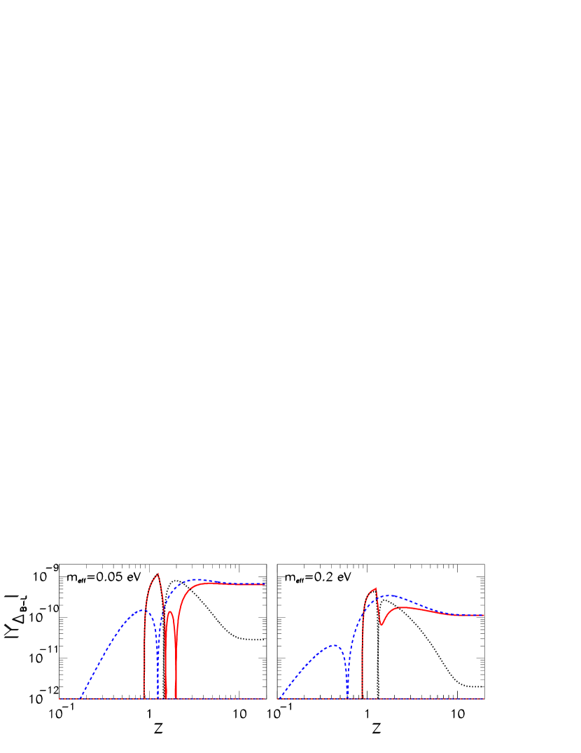
Figure 18: Evolution of $Y_{\Delta_{B-L}}$. The solid continuous (red) lines depict the complete results in the $m_{\widetilde{g}}=\mu\to 0\,$ limit. The dashed (blue) lines correspond to the same limit when thermal corrections to the $CP$ asymmetries are neglected. The dotted (black) lines gives $Y_{\Delta_{B-L}}$ with thermal effects when SE is assumed. The picture on the left is for $m_{\rm eff}=0.05\,$eV and that on the right for $m_{\rm eff}=0.20\,$eV.

Fig. 18 displays the evolution of $Y_{\Delta_{B-L}}$ with increasing $z=M/T$. The solid (red) lines correspond to the full results obtained in the $m_{\widetilde{g}},\,\mu\to 0\,$GeV limit, that is when particle-sparticle superequilibrating processes are completely switched off. The dashed (blue) lines give the results obtained in the same limit, but when all thermal corrections to the CP asymmetries are neglected, and $\epsilon^{s}=-\epsilon^{f}=\bar{\epsilon}/2$. Both pictures display clearly that in the NSE regime neglecting thermal corrections in evaluating the final values of $Y_{\Delta_{B-L}}$ is an excellent approximation. The dotted (black) lines give $Y_{\Delta_{B-L}}$ with thermal corrections included and under the assumption of SE, that in the BE (210)-(211) corresponds to taking the limit $m_{\widetilde{g}},\mu\to\infty$. The two panels are for two different washout strengths $m_{\rm eff}=0.05\,$eV (left) and $m_{\rm eff}=0.20\,$eV (right) and, as anticipated, they show that stronger washouts result in larger gain in the efficiency.

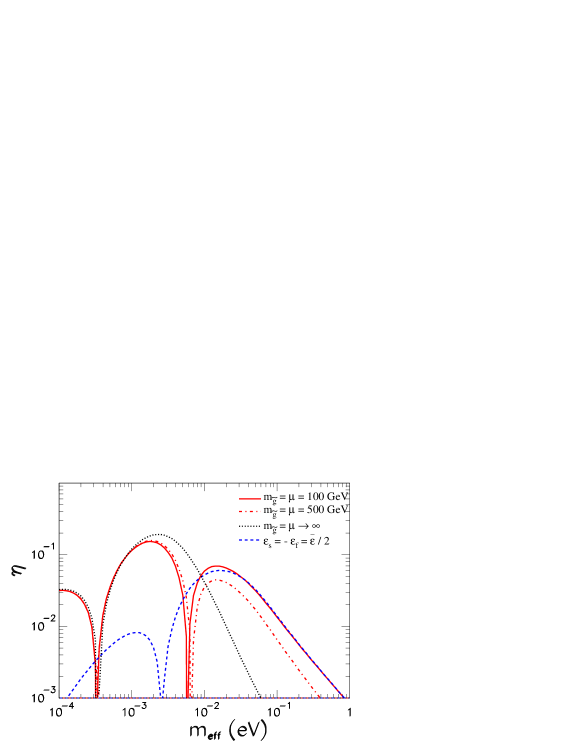
Figure 19: Efficiency factor $\eta$ as a function of the washout parameter $m_{\rm eff}$ for Case I ($h_{e,d}$ Yukawa equilibrium) and different values of $m_{\widetilde{g}}=\mu$. The red continuous line is for the NSE regime with $m_{\widetilde{g}}=\mu=100\,$GeV. The dashed blue line give the result for the same regime when thermal corrections are neglected. The red dash-dotted line corresponds to $m_{\widetilde{g}}=\mu=500\,$GeV, and the black dotted line to SE with $m_{\widetilde{g}},\,\mu\to\infty$.

Fig. 19 shows the efficiency $\eta$ as a function of the washout parameter $m_{\rm eff}$. The red continuous line corresponds to $m_{\widetilde{g}}=\mu=100\,$GeV, and since it is practically indistinguishable from the $m_{\widetilde{g}}=\mu\to 0\,$ case, the evolution occurs in the NSE regime in agreement with Eq. (170). The red dash-dotted line corresponds to $m_{\widetilde{g}}=\mu=500\,$ GeV. In this case we see that SE rates start suppressing the efficiency even without attaining full thermal equilibrium. The black dotted line corresponds to the $m_{\widetilde{g}},\,\mu\to\infty\,$ limit of complete SE. The figure illustrates that at $T\ \hbox to0.0pt{\raise 3.0pt\hbox{$>$}\hss}{\lower 3.0pt\hbox{$\sim$}}\ 10^{7}\,$GeV the leptogenesis efficiency could be significantly underestimated if SE is incorrectly assumed. The size of this underestimation is a fast increasing function of the washouts, and for particularly large values of $m_{\rm eff}$ can reach the two orders of magnitude level. Also, for $m_{\rm eff}\ \hbox to0.0pt{\raise 3.0pt\hbox{$>$}\hss}{\lower 3.0pt\hbox{$\sim$}}\ 6\times 10^{-3}\,$eV, the assumption of SE results in a baryon asymmetry of the wrong sign. Graphically, one can see this from the fact that at small values of $m_{\rm eff}$ the black dotted and red dash-dotted and continuous lines approximately overlap, and there is a change of sign in $Y_{\Delta B-L}^{\infty}/\bar{\epsilon}$ around $m_{\rm eff}\sim 3\times 10^{-4}\,$eV. But around $m_{\rm eff}\sim 6\times 10^{-3}\,$eV for the red dash-dotted and continuous lines there is another sign change. This marks the onset of $R$-genesis domination; therefore, from this point onward, baryogenesis does not proceed through leptogenesis, but rather through $R$-genesis. In the same figure the dashed blue continuous line shows the NSE results in the approximation of neglecting all thermal corrections to the $CP$ asymmetries. By comparing with the full results (red continuous line) we see that for $m_{\rm eff}\ \hbox to0.0pt{\raise 3.0pt\hbox{$>$}\hss}{\lower 3.0pt\hbox{$\sim$}}\ {\rm few}\,\times 10^{-2}\,$eV thermal corrections give negligible effects. Thus, for $R$-genesis, the zero temperature approximation yields quite reliable results.

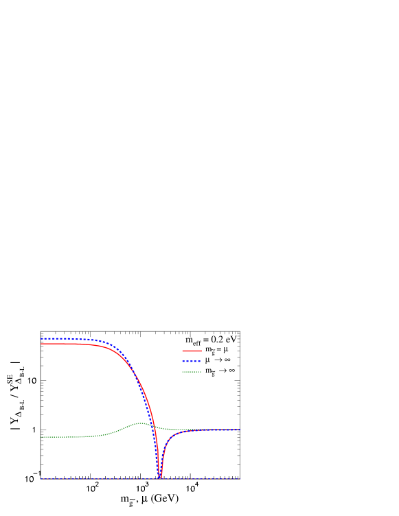
Figure 20: The final value of $Y_{\Delta_{B-L}}$ normalized to the SE result $Y^{SE}_{\Delta_{B-L}}$ as a function of $m_{\widetilde{g}}$ and $\mu$ for Case I ($h_{e,d}$ Yukawa equilibrium) and $m_{\rm eff}=0.20\,$eV. The red continuous line corresponds to varying simultaneously both parameters holding $m_{\widetilde{g}}=\mu$. The blue dashed line corresponds to varying only $m_{\widetilde{g}}$ with $\mu\to\infty$. The green dotted line corresponds to varying only $\mu$ with $m_{\widetilde{g}}\to\infty$.

Fig. 20 displays the value of $Y_{\Delta_{B-L}}^{\infty}$ (labeled just as $Y_{\Delta_{B-L}}$ for simplicity) as a function of different values of $m_{\widetilde{g}}$ and $\mu$, normalized to $Y^{SE}_{\Delta_{B-L}}$ that is the final value of the asymmetry obtained assuming SE. In order to enhance the impact of the new effects, the washout parameter has been fixed to a rather large value $m_{\rm eff}=0.20\,$eV. The red continuous line corresponds to varying simultaneously both SE parameters keeping their values equal: $m_{\widetilde{g}}=\mu$. We see that for $m_{\widetilde{g}}=\mu\ \hbox to0.0pt{\raise 3.0pt\hbox{$<$}\hss}{\lower 3.0pt\hbox{$\sim$}}\ 1\,$TeV the amount of $B-L$ asymmetry produced by SL can be up to two orders of magnitude larger (and of the opposite sign) with respect to what would be obtained in the usual approach with SE. SE effects start suppressing the asymmetry around $m_{\widetilde{g}}=\mu\sim 1\,$TeV. The asymmetry then changes sign around $3\,$TeV, that marks the transition from the $R$-genesis to the leptogenesis regime, and eventually around $5\,$TeV SE reactions attain complete thermal equilibrium and $Y_{\Delta_{B-L}}/Y^{SE}_{\Delta_{B-L}}\to 1$.

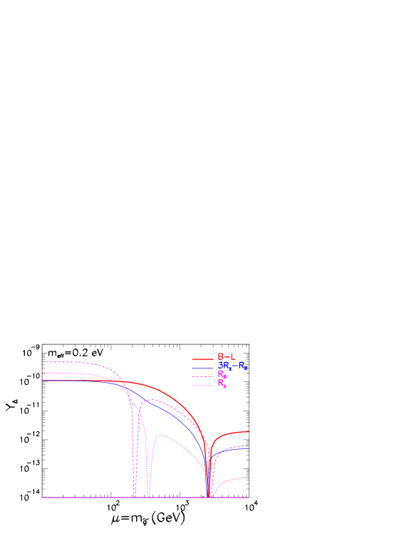
Figure 21: Final values of the charge density asymmetries as a function of $m_{\widetilde{g}}=\mu$ for Case I ($h_{e,d}$ Yukawa equilibrium) and $m_{\rm eff}=0.20\,$eV. Thick red line: $Y_{\Delta_{B-L}}$; thick blue line: $3Y_{\Delta R_{\chi}}-Y_{\Delta R_{B}}$; thin dashed purple line: $Y_{\Delta{R_{B}}}$; thin dotted purple line: $Y_{\Delta{R_{\chi}}}$.

The BE (210)-(211) are general enough to allow to study what would happen if only one of the two anomalous symmetries $U(1)_{R}$ or $U(1)_{PQ}$ were present. The corresponding results are also depicted in Fig. 20. The blue dashed line corresponds to the $U(1)_{R}$-theory where $m_{\widetilde{g}}$ is varied while $U(1)_{PQ}$ is broken. The green dotted line corresponds to the alternative $U(1)_{PQ}$-theory in which $m_{\widetilde{g}}\to\infty$ and only $\mu$ is varied. These results clearly show that the real responsible of the large effects is the $R$-symmetry, while the effects of the $PQ$ symmetry remains qualitatively more at the level of typical spectator effects. A theoretical justification of this behavior is not difficult to find, and we will discuss it in the following section.

Some important aspects of the transition from $R$-genesis (NSE regime) to leptogenesis (SE regime) are highlighted in Fig. 21 which displays the final value of the relevant charge density asymmetries as a function of $m_{\widetilde{g}}=\mu$, assuming Case I and $m_{\rm eff}=0.20\,$eV. The thick solid red line corresponds to $Y_{\Delta_{B-L}}$, while the thin solid blue line corresponds to $3Y_{\Delta R_{\chi}}-Y_{\Delta R_{B}}$. The thin dashed and dotted purple lines display respectively $Y_{\Delta{R_{B}}}$ and $Y_{\Delta{R_{\chi}}}$. We see that up to $m_{\widetilde{g}}=\mu\sim 100\,$GeV we have $Y_{\Delta_{B-L}}\simeq 3Y_{\Delta R_{\chi}}-Y_{\Delta R_{B}}$ that is in agreement with Eq. (217), and thus implies that baryogenesis occurs almost only via $R$-genesis. As the soft SUSY-breaking parameters are increased, SE reactions begin to wash out efficiently $Y_{\Delta{R_{B}}}$ and $Y_{\Delta{R_{\chi}}}$ but the difference $3Y_{\Delta{R_{\chi}}}-Y_{\Delta{R_{B}}}$ still remains of the order of $Y_{\Delta_{B-L}}$, and $R$-genesis still gives the dominant contribution to baryogenesis. Around $m_{\widetilde{g}}=\mu\sim 3\,$TeV all the charge asymmetries change simultaneously their sign. This is the benchmark of the onset of the regime in which leptogenesis dominates. The only relevant source for generating the density-asymmetries is now the (opposite-sign) thermally induced $B-L$ asymmetry, that is not affected by SE washouts, and that is feeding (small) asymmetries into all the other charges. In this regime $Y_{\Delta_{R_{B}}}$ and $Y_{\Delta_{R_{\chi}}}$ do not have anymore an independent dynamics, and can be simply computed in terms of $Y_{\Delta_{B-L}}$ yielding $Y_{\Delta{R_{B}}}=-\frac{1}{3}Y_{\Delta_{B-L}}$ and $Y_{\Delta{R_{\chi}}}=-\frac{3}{79}\,Y_{\Delta_{B-L}}$.

6.6 Discussion

In the temperature regime quantified by Eq. (170) all reactions that depend on the soft gaugino masses do not occur. In this regime the early Universe effective theory includes a new $R$-symmetry. In SL, this $R$-symmetry is violated in the out of equilibrium interactions of RHN and RHSN. In particular, $R$-number CP asymmetries in heavy RHSN decays can be defined, and constitute important quantities. In fact, given that $R$-symmetries do not commute with SUSY transformations, it is hardly surprising that no cancellation occurs between the $R$-number CP asymmetries for scalars and fermions. For this reason, a sizable density asymmetry for the $R$ charge can develop in the thermal bath, and this asymmetry turns out to play the main role for the generation of the baryon asymmetry.

To keep higgsinos sufficiently light, in SUSY one needs to assume $\mu\sim m_{\tilde{g}}$, and thus when the gaugino masses are set to zero, one must set $\mu\to 0$ as well. In this limit the effective theory acquires another quasi-conserved global symmetry, that is a $U(1)_{PQ}$ symmetry of the Peccei-Quinn type. $PQ$ is also violated in RHSN interactions and thus it also has an associated CP asymmetry. However, since $U(1)_{PQ}$ is a bosonic symmetry that commutes with SUSY, the same cancellation between fermion/boson $CP$ asymmetries occurring for lepton number also occurs for $PQ$. Accordingly, $PQ$ does not play an equivalently important role in the generation of the baryon asymmetry.

In order to make more understandable the previous two remarks, let us start from the beginning, by listing the relevant global symmetries of the effective theory. For simplicity we concentrate on Case I ($h_{e,d}$ Yukawa equilibrium). Neglecting lepton flavour, that is irrelevant for the present discussion, these symmetries are: $L,\,R,\,PQ,\,B$ and $\raise 2.0pt\hbox{$\chi$}_{u^{c}_{L}}$. The first three $L,\,R,\,PQ$ are violated perturbatively in the interactions of the RHSN, and all five symmetries are violated by non-perturbative sphaleron processes. In this review, in carrying out our analysis, we have first identified the anomaly free combinations of the five charges, that are $B-L$, $R_{B}$ and $R_{\chi}$, and then we have written down the BE to describe their evolutions. Here, we want to sketch a different procedure. We first write a set of evolution equations for the five anomalous charges, that have the form:

$$\dot{Y}_{\Delta_{\cal Q}}={\cal S}_{\Delta_{\cal Q}}+{\cal G}_{\Delta_{\cal Q}}+{\cal G}^{NP}_{\Delta_{\cal Q}}\,.$$ (223)

In this equation ${\cal S}$ represents the source term for $Y_{\Delta}$, ${\cal G}$ is the (s)neutrino-related washouts with all density-asymmetries and signs absorbed, and ${\cal G}^{NP}$ represents the non-perturbative EW and/or QCD sphaleron reactions that violate $\Delta_{\cal Q}$. The latter are reactions of type (i) discussed in the introduction in Section 3.1 and in this Section in 6.2, that is fast processes, that eventually will be convenient to eliminate in favour of chemical equilibrium conditions. Now, given that $B$ and $\raise 2.0pt\hbox{$\chi$}_{u^{c}_{L}}$ are good symmetries at the perturbative level, they have no CP-violating source terms: ${\cal S}_{\Delta_{B}},\,{\cal S}_{\Delta_{\chi}}=0$ (they also do not have perturbative washouts, and ${\cal G}_{\Delta_{B}}$ ${\cal G}_{\Delta_{\chi}}=0$ too). The only source terms thus are ${\cal S}_{\Delta_{L}},\,{\cal S}_{\Delta_{PQ}}$ and ${\cal S}_{\Delta_{R}}$. However, as we already know, in the $T\to 0$ limit, for ${\cal S}_{\Delta_{L}}$ we have a cancellation between the fermion and scalar contributions: ${\cal S}^{f}_{\Delta_{L}}+{\cal S}^{s}_{\Delta_{L}}\to 0$. This straightforwardly implies that ${\cal S}^{f}_{\Delta_{PQ}}+{\cal S}^{s}_{\Delta_{PQ}}\to 0$ too, since the RHSN processes contributing to the CP asymmetry for $PQ$ are the same as for $L$: they are simply multiplied by the appropriate $PQ$ charge that is, however, the same for fermion and scalar final states. For the $R$ charge we have instead ${\cal S}_{\Delta_{R}}\propto R_{f}\cdot{\cal S}^{f}_{\Delta_{L}}+R_{s}\cdot{\cal S}^{s}_{\Delta_{L}}$, where $R_{f,s}$ are respectively the overall $R$-charges of the fermion and boson two particle final states, and thus satisfy $R_{s}=R_{f}+2$. We then straightforwardly obtain that in the $T\to 0$ limit the $R$-charge source term does not vanish, and is given by ${\cal S}_{\Delta_{R}}\to 2\,{\cal S}^{s}_{\Delta_{L}}$. Fast in-equilibrium sphaleron processes enforce equilibrium conditions between particle densities carrying $R$ charge, and those carrying a $B$ and $L$ numbers and, as a result, baryon and lepton asymmetries roughly of the same order than the $R$ charge-asymmetry develop. Eventually, with the decreasing of the temperature, gaugino mass related reactions will start occurring with in-equilibrium rates erasing any asymmetry in the $R$ charge. It is important to notice that when the $R$-symmetry gets explicitly broken, generalized EW sphalerons reduce to the standard EW sphalerons, and sphaleron induced multi-fermion operators decouple from gauginos, and reduce to their standard $B+L$ violating form. Since gaugino mass reactions as well as all other MSSM processes conserve $B-L$, the asymmetry initially generated through $R$-genesis will remain unaffected.

Now that we have identified where the large density asymmetries come from, we can complete our procedure by constructing suitable linear combinations of the five equations (223) for which the sphaleron terms ${\cal G}^{NP}$ cancel out. Since there are only two such terms, ${\cal G}^{NP}_{EW}$ and ${\cal G}^{NP}_{QCD}$, we can construct three linear combinations in which only processes of type (iii) enter. These are the BE for the three anomaly free charges that have been discussed at length in Section 6.1. The equilibrium conditions enforced by ${\cal G}^{NP}_{EW}$ and ${\cal G}^{NP}_{QCD}$ have to be imposed on the system, and to obtain the BE in closed form, the various density-asymmetries appearing in the washout terms ${\cal G}$ must be rotated into the densities of the anomaly free charges by means of an appropriate $A$ matrix.

7 Soft Leptogenesis Testability and Variations

As is well-known, leptogenesis models are plagued with the undesirable feature that their experimental verification is very difficult, and in minimal scenarios it appears to be impossible, at least in the light of foreseeable experimental tests. This is because, to establish leptogenesis experimentally, we would need to produce the heavy states responsible for the generation of the lepton asymmetry, and measure the CP asymmetry in their decays. With the dawn of the LHC, this issue has been more pressing than ever, since new states with masses of the order of the TeV could become for the first time accessible. However, in the most natural scenarios, the new states relevant for leptogenesis lie at a scale that is several orders of magnitude above the TeV. With some severe fine tuning, masses light enough to fall within the energy range accessible at the LHC could be accommodated. However, in this case to keep the light neutrino mass scale within the experimental limits the Yukawa couplings of the heavy states must be extremely tiny, preventing again any possibility of direct production. The possibility of indirect verifications of leptogenesis, for example by pinning down the whole set of the eighteen parameters of the seesaw, and from this deriving a prediction for the baryon asymmetry, is also not viable. This is because only half of the seesaw parameters are (in principle) accessible at low energy, while the values of some of the remaining (unmeasurable) high energy parameters are crucial for leptogenesis predictions.

As regards SL, it is clear that the discovery of SUSY at the LHC can be regarded as a basic condition to keep considering this scenario as a possible explanation of the cosmic baryon asymmetry. However, in spite of an energy scale that is intrinsically much lower than that of standard leptogenesis, and that could even fall within the range of energies accessible at the LHC, with respect to the possibility of direct experimental verifications SL is in no better shape than standard (or supersymmetric) leptogenesis. Even if the RHSN mass is low enough, direct production of RHSN faces the same no-go issue of extremely suppressed couplings. Indirect evidences could in principle come from measurements unrelated to the neutrino sector because, as it has been thoroughly discussed in Section 2, SL depends also on soft SUSY-breaking parameters that are not directly related with the seesaw. These parameters could in principle be measurable through their effects on other low energy observables like LFV lepton decays, or the electric dipole moments of the charged leptons, that receive contributions from the complex phases of the soft SUSY-breaking terms. However, Ref. Kashti:2004vj that addressed specifically this issue, found that all the related effects are much smaller than other MSSM contributions, and therefore unobservable. One can thus conclude that, much alike standard leptogenesis and supersymmetric leptogenesis, the simplest SL scenario based on the supersymmetric type I seesaw, and on the related soft SUSY-breaking terms, also escapes the possibility of experimental verification.

7.1 Variations of soft leptogenesis

The exceedingly strong suppression of the production rates of relatively light RHSN states is clearly the direct consequence of their gauge-singlet nature, that leaves the tiny Yukawa interactions as the only mechanism for their production. In order to obviate this problem one can assume that these states are non-singlet under $SU(2)_{L}$, or under some new gauge symmetry, so that they could be produced at colliders through the corresponding gauge interactions. However, in following this approach, one has to be very careful because fast gauge scatterings could potentially keep the RHSN in complete thermal equilibrium, and/or RHSN annihilation through gauge boson channels could leave a too small fraction of out-of-equilibrium decaying states.

In Refs. D’Ambrosio:2004fz,Chun:2005ms the MSSM with the addition of an $SU(2)_{L}$ triplet of scalars with non-zero hypercharge (as required for the type II seesaw) was considered, and the possibility of SL at a low scale was investigated. Fast annihilations of the scalar triplets through gauge interactions keep the triplet abundance very close to its equilibrium value, and strongly suppress the final lepton asymmetry. However, it is argued that for a triplet mass scale $10^{3}-10^{4}\,{\rm GeV}$ leptogenesis could still be successful.[128] Due to the small neutrino Yukawa coupling $\sim 10^{-6}$ all low-energy LFV processes like $\mu\to e\gamma$ or $\mu\to 3e$ remain strongly suppressed.[129, 130] On the other hand, Tevatron and LHC have the potential to produce these triplets, and a marked signature will be the decay of the doubly charged component of the triplet to lepton and Higgsino pairs.[131, 132]

A supersymmetric seesaw model associated with an extra $U(1)^{\prime}$ gauge symmetry spontaneously broken at the TeV scale has been studied in Ref. Chun:2005tg, and shown to be a viable option for the generation of the cosmological baryon asymmetry via the SL mechanism. Such a scenario leads to testable predictions in colliders, through the production of $Z^{\prime}$ and their subsequent decays into RHSN. The RHSN will further decay to final states with pairs of same-sign leptons (sleptons) and charginos (charged Higgses) through $\widetilde{N}-\widetilde{N}^{*}$ mixing and CP violation.

SL in the inverse seesaw model was considered in Ref. Garayoa:2006xs. This is another interesting possibility with the potential of being verified experimentally. In this scenario the lightness of the active neutrinos is not associated with tiny neutrino Yukawa couplings, but with a small dimensional parameter that breaks $U(1)_{L}$. The unsuppressed Yukawa couplings together with a low mass scale for the RHSN can result in a relatively large mixing with the SM leptons, and through this mixing direct production and detection of the RHSN at the LHC become possible.

Ref. Medina:2006hi put forth the more speculative idea of implementing SL in a warped five dimensional scenario. It was shown that, within the context of extra dimensions, the condition of out-of-equilibrium decay and the phenomenological constraints on the neutrino mass can be both satisfied in a natural way, and that all necessary elements needed for SL to predict a correct value for the baryon asymmetry can be obtained. While the specific SL mechanism of this model does not seem to be easily verifiable experimentally, the general idea of extra dimensions could potentially be probed at LHC through the production of the Kaluza-Klein excitations. An experimental confirmation of this scenario would certainly increase the phenomenological interest of SL in the context of extra dimensions.

Other interesting alternative models which utilize soft-SUSY breaking terms to realize leptogenesis at a low scale have been considered in Refs. Allahverdi:2004ix,Boubekeur:2004ez,Ellis:2005uk. It remains to be seen if any of these models can yield some clear experimental signature.

8 Final Remarks and Conclusions

The matter-antimatter asymmetry of the Universe and the experimental confirmation of tiny but non-vanishing neutrino masses are two among the very few evidences of physics beyond the Standard Model. The type I seesaw can elegantly explain the strong suppression of the neutrino mass scale, and through the leptogenesis mechanism can also provide a natural explanation of the cosmic matter-antimatter asymmetry. Leptogenesis can be quantitatively successful without any fine-tuning of the seesaw parameters, yet, in the non-supersymmetric seesaw framework, a fine-tuning problem arises due to the large corrections to the mass-squared parameter of the Higgs potential, that are proportional to the heavy Majorana neutrino masses. The supersymmetric version of the seesaw has the virtue of stabilizing the Higgs mass-squared parameter under radiative corrections, but at the same time also introduces a serious tension between the lower limit on the seesaw scale that follows from the requirement of successful baryogenesis, and the upper bound on the reheating temperature that must be satisfied to avoid an overproduction of gravitinos.

However, supersymmetry (SUSY) has to be broken, and this yields the possibility that leptogenesis could proceed through right-handed sneutrino decays, thanks to the new sources of CP violation from complex phases in the SUSY-breaking sector. In this scenario the leptogenesis scale is naturally lowered and successful baryogenesis can be obtained anywhere in the temperature range $10^{4}\,{\rm GeV}\lesssim T\lesssim 10^{9}\,{\rm GeV}$. Accordingly, the tension with the gravitino problem gets generically relaxed and, in the lower temperature window, is completely avoided. This scenario, termed soft leptogenesis[50, 51] (SL) has been the subject of this review.

As discussed in Section 2, SL is plagued by the problem of a congenital low efficiency, that is related to the cancellation between the asymmetries produced in fermions and bosons carrying lepton number. It should be stressed that it is the fact that lepton number commutes with supersymmetric transformations (that is that scalar and fermionic members of the lepton supermultiplets have the same lepton charge) that plays the crucial role in enforcing this cancellation. Finite temperature corrections break SUSY spoiling the cancellation between the scalar and fermionic CP asymmetries, and can eventually rescue SL from a complete failure.

The basic mechanism of SL was reviewed in Section 3. To highlight the role of thermal factors and of the different types of CP asymmetries, in this section the simplifying assumptions of a single lepton flavour and of equal density asymmetries for the lepton and slepton states (superequilibration) were adopted.

When the SL CP asymmetries are dominated by the contribution from mixing, the RHSN have to be highly degenerated, and in this situation quantum effects can become important. These issues have been reviewed in Section 4. In the strong washout regime quantum effects can enhance the absolute value of the final asymmetry and also induce a change of its sign. However, altogether, the allowed parameter space for SL to be successful is not modified substantially.

Issues related with lepton flavour effects have been addressed in Section 5. Given that SL can only occur at temperatures low enough that all the three lepton flavours are resolved by their fast charged lepton Yukawa interactions, the inclusion of flavour effects in SL studies is mandatory. We have seen that enhancements of the produced asymmetry up to factors $\sim 10^{3}$ are possible when flavour effects are accounted for, and this is sufficient to avoid the need of additional enhancements from resonant conditions. Thus, the RHSN do not need to be highly degenerated, and a natural scale for the sneutrino mixing parameter $B\sim m_{SUSY}$ is allowed.

In Section 6 we discussed the recently discovered possibility that baryogenesis could proceed through $R$-genesis.[72] If the RHSN mass lies above $M\sim 10^{7}\,$GeV, a new scenario different from SL must be considered. In this scenario the asymmetry is first generated in a new $R$ charge that is conserved in the effective theory when all gaugino-related reactions can be neglected, which is the case when $T\ \hbox to0.0pt{\raise 3.0pt\hbox{$>$}\hss}{\lower 3.0pt\hbox{$\sim$}}\ 10^{7}\,$GeV. This asymmetry is then transferred in part to baryons via generalized electroweak sphaleron interactions. Given that $R$-symmetries do not commute with SUSY transformations, the scalar and fermionic members of the lepton supermultiplets have different $R$-charges, and no cancellation between the $R$-asymmetries produced in fermions and bosons occurs. Thus, in the high temperature window where SL is replaced by $R$-genesis, a sizable baryon asymmetry can be generated regardless of thermal effects.

In conclusion, SUSY allows for baryogenesis via leptogenesis to occur at any temperature from somewhat below the GUT scale down to the TeV. Above $T\sim 10^{9}\,{\rm GeV}$ baryogenesis can occur through the supersymmetric version of standard leptogenesis, although this possibility is disfavoured by considerations related to gravitino overproduction, whose decays would affect Big Bang nucleosynthesis. In the intermediate temperature range $10^{7}\,{\rm GeV}\lesssim T\lesssim 10^{9}\,{\rm GeV}$, where the gravitino constraint gets relaxed, baryogenesis can occur through $R$-genesis, which is a highly efficient mechanism in which the production of asymmetries does not rely on thermal effects. In the lower temperature window $T\lesssim 10^{7}\,{\rm GeV}$ where the gravitino problem is usually evaded, the usual SL mechanism can take place, with an efficiency that is suppressed by the scalar-boson asymmetries cancellation, but with possible large enhancements from flavour effects. Finally, carefully constructed variations of SL can allow for a scale as low as the TeV and, as was briefly reviewed in Section 7.1, in some of these cases experimental verifications are also possible.

Appendix A Boltzmann Equations

A.1 General Boltzmann equations

Our Universe is very well described by a spatially homogeneous and isotropic metric known as Robertson-Walker (RW) metric

$$ds^{2}=dt^{2}-R^{2}(t)\left[\frac{dr^{2}}{1-kr^{2}}+r^{2}d\theta^{2}+r^{2}\sin^{2}\theta d\phi^{2}\right],$$ (224)

where $(t,r,\theta,\phi)$ are comoving coordinates, $R(t)$ is the cosmic scale factor, and $k=0,+1,-1$ describe spaces of zero, positive, or negative spatial curvature, respectively. For a general process $a+b+...\leftrightarrow i+j+....$ in the RW space, the Boltzmann equation (BE) for the phase-space distribution of the particle species $a$ can be written as:

$$\frac{\partial f_{a}}{\partial t}-H\,|\vec{p}_{a}|\,\frac{\partial f_{a}}{\partial|\vec{p}_{a}|} = -\frac{1}{2E_{a}}C[f_{a}],$$ (225)

where

$$C[f_{a}] \equiv \frac{1}{g_{a}}\sum_{b,...i,j,...}\Lambda_{b...}^{ij...}\left[\left|\mathcal{M}\left(ab...\rightarrow ij...\right)\right|^{2}f_{a}f_{b}...\left(1+\eta_{i}f_{i}\right)\left(1+\eta_{j}f_{j}\right)...\right.$$ (226)

$$\left.-\left|\mathcal{M}\left(ij...\rightarrow ab...\right)\right|^{2}f_{i}f_{j}...\left(1+\eta_{a}f_{a}\right)\left(1+\eta_{b}f_{b}\right)...\right].$$

In the above $g_{a}$ is the number of spin degrees of freedom of particle $a$ and

$$\Lambda_{b...}^{ij...}\! \equiv \!\!\int d\Pi_{b}...d\Pi_{i}d\Pi_{j}...\left(2\pi\right)^{4}\delta^{\left(4\right)}\left(p_{a}+p_{b}+...-p_{i}-p_{j}-...\right),$$

$$d\Pi_{x} \equiv \frac{d^{3}p_{x}}{\left(2\pi\right)^{3}2E_{x}}.$$ (227)

In Eq. (226), $\left|\mathcal{M}_{ab...\rightarrow ij...}\right|^{2}$ is the squared amplitude summed over initial and final quantum numbers (spin states and gauge multiplicity) and $f_{x}$ is the distribution function of $x$ with $\eta_{x}=\pm$ if $x$ is a boson or fermion respectively. The factors $(1\pm f_{x})$ are known as Pauli-blocking (for $x$ being fermion) and Bose-enhancement or stimulated emission (for $x$ being boson) factors, respectively. In Eq. 225, the Hubble expansion rate of the Universe $H$ in the radiation-dominated era is given by

$$H \equiv \frac{\dot{R}}{R}=\frac{2}{3}\sqrt{\frac{g_{*}\pi^{3}}{5}}\frac{T^{2}}{M_{pl}},$$ (228)

where $M_{pl}=1.22\times 10^{19}\,$GeV is the Planck mass, $g_{*}$ is the total number of relativistic degrees of freedom ($g_{*}=228.75$ for MSSM).

Using the definition of the number density in terms of the phase space distribution

$$n_{a}=g_{a}\int\frac{d^{3}p}{(2\pi)^{3}}f_{a},$$ (229)

and upon integration by parts, the BE (225) can be rewritten in the form

$$\frac{dn_{a}}{dt}+3Hn_{a} = -\sum_{b,...i,j,...}\left[ab...\leftrightarrow ij...\right],$$ (230)

where

$$\left[ab...\leftrightarrow ij...\right] \equiv \Lambda_{ab...}^{ij...}\left[\left|\mathcal{M}\left(ab...\rightarrow ij...\right)\right|^{2}f_{a}f_{b}...\left(1+\eta_{i}f_{i}\right)\left(1+\eta_{j}f_{j}\right)...\right.$$ (231)

$$\left.-\left|\mathcal{M}\left(ij...\rightarrow ab...\right)\right|^{2}f_{i}f_{j}...\left(1+\eta_{a}f_{a}\right)\left(1+\eta_{b}f_{b}\right)...\right].$$

Notice that in writing the BE (230), we have implicitly assumed that the right hand side of this equation can also be written in term of $n_{a}$. However, without certain approximations, this cannot be done in general and we have to resort to the BE (225) and solve it in term of phase space distribution. In A.2.1 we list the approximations that allow us to write the right hand side of Eq. (230) in terms of number densities, and then to use the BE (230).

In order to scale out the effect of the expansion of the Universe. one defines the particle abundance i.e. the particle density $n_{a}$ normalized to the entropy density $s$ as:

$$Y_{a}\equiv\frac{n_{a}}{s},$$ (232)

where the entropy density in the radiation dominated era is given by

$$s=\frac{2\pi^{2}}{45}g_{*}T^{3}.$$ (233)

Using the conservation of entropy per comoving volume (i.e. $s\,R^{3}=$ constant), replacing the time $t$ with the temperature $T$ (in the radiation dominated era $t=\frac{1}{2H}\sim T^{-2}$) and defining the dimensionless parameter

$$z\equiv\frac{M}{T},$$ (234)

where $M$ is any convenient mass scale, the left hand side of Eq. (230) becomes:

$$\frac{dn_{a}}{dt}+3Hn_{a}=s\frac{dY_{a}}{dt}=sHz\frac{dY_{a}}{dz}.$$ (235)

Regarding the distribution functions in Eqs. (231), for particles for which the elastic scatterings are much faster than the inelastic scatterings, one can assume that they are in kinetic equilibrium and have either Fermi-Dirac distribution (for fermions $f$) or Bose-Einstein distribution (for scalars $s$) given respectively by

$$f_{f,\overline{f}}=\frac{1}{e^{\left(E_{f}\mp\mu_{f}\right)/T}+1},\;\;\;\;\;f_{s,s^{*}}=\frac{1}{e^{\left(E_{s}\mp\mu_{s}\right)/T}-1},$$ (236)

where $\mu$’s are the chemical potentials and the “bar” or “star” refers to the corresponding antiparticles. The equilibrium distributions $f^{eq}_{x}$ are defined as those with $\mu=0$:

$$f_{f,\overline{f}}^{eq}=\frac{1}{e^{E_{f}/T}+1},\;\;\;\;\;f_{s,s^{*}}^{eq}=\frac{1}{e^{E_{s}/T}-1}.$$ (237)

So for $\frac{\mu}{T}\ll 1$ one can expand the kinetic equilibrium distribution function in $\frac{\mu}{T}$ as

$$f_{f,\overline{f}} = f_{f}^{eq}\pm f_{f}^{eq,2}e^{E_{f}/T}\frac{\mu_{f}}{T}+\mathcal{O}\left[\left(\frac{\mu_{f}}{T}\right)^{2}\right],$$

$$f_{s,s^{*}} = f_{s}^{eq}\pm f_{s}^{eq,2}e^{E_{s}/T}\frac{\mu_{s}}{T}+\mathcal{O}\left[\left(\frac{\mu_{s}}{T}\right)^{2}\right].$$ (238)

It follows that

$$f_{f}-f_{\overline{f}} = 2\left(1-f_{f}^{eq}\right)f_{f}^{eq}\frac{\mu_{f}}{T}+\mathcal{O}\left[\left(\frac{\mu_{f}}{T}\right)^{3}\right],$$

$$f_{s}-f_{s^{*}} = 2\left(1+f_{s}^{eq}\right)f_{s}^{eq}\frac{\mu_{s}}{T}+\mathcal{O}\left[\left(\frac{\mu_{s}}{T}\right)^{3}\right],$$ (239)

where we have used the identities

$$1-f_{f,\overline{f}}=e^{(E_{f}\mp\mu_{f})/T}f_{f,\overline{f}},\;\;\;\;\;1+f_{s,s^{*}}=e^{(E_{s}\mp\mu_{s})/T}f_{s,s^{*}}.$$ (240)

Using Eq. (229) one gets that the difference between number densities of massless particles and antiparticles at leading order in chemical potentials is

$$n_{\Delta f}\equiv n_{f}-n_{\overline{f}}=\frac{g_{f}}{6}T^{3}\frac{\mu_{f}}{T},\;\;\;\;\;n_{\Delta s}\equiv n_{s}-n_{\bar{s}}=\frac{g_{s}}{3}T^{3}\frac{\mu_{s}}{T}.$$ (241)

Defining the density asymmetries per degree of freedom $Y_{\Delta f,s}\equiv n_{\Delta f,s}/(g_{f,s}s)$ as the the number density asymmetries per degree of freedom $n_{\Delta f,s}/g_{f,s}$ normalized to the entropy density $s$, we can rewrite the chemical potentials for massless fermions and bosons as:

$$2\frac{\mu_{f}}{T}=\frac{8\pi^{2}g_{*}}{15}Y_{\Delta f}\equiv\frac{Y_{\Delta f}}{Y_{f}^{eq}},\;\;\;\;\;2\frac{\mu_{s}}{T}=\frac{4\pi^{2}g_{*}}{15}Y_{\Delta s}\equiv\frac{Y_{\Delta s}}{Y_{s}^{eq}},$$ (242)

where $Y_{f}^{eq}\equiv\frac{15}{8\pi^{2}g_{*}}$ and $Y_{s}^{eq}\equiv\frac{15}{4\pi^{2}g_{*}}$.

Let us introduce the following shorthand notation:

$$F_{ab...ij...}\left(...\right) \equiv \Lambda_{ab...}^{ij...}\left|\mathcal{M}\left(ab...\rightarrow ij...\right)\right|^{2}\left(...\right),$$

$$\overline{F_{ab...ij...}}\left(...\right) \equiv \Lambda_{ab...}^{ij...}\left|\mathcal{M}\left(ij...\rightarrow ab...\right)\right|^{2}\left(...\right),$$ (243)

where $(...)$ denotes some function to be integrated over. Note that CPT invariance implies $\overline{F_{ab...ij...}}\left(...\right)=F_{\overline{ab...ij...}}\left(...\right)$. The thermally averaged reaction densities can be defined as

$$\gamma\left(ab...\rightarrow ij...\right)\! \equiv \!F_{ab...ij...}\times f_{a}^{eq}f_{b}^{eq}...\left(1+\eta_{i}f_{i}^{eq}\right)\left(1+\eta_{j}f_{j}^{eq}\right)...,\qquad$$ (244)

where we have used the equilibrium distribution functions with vanishing chemical potentials Eqs. (237).

Neglecting Pauli-blocking and Bose-enhancement factors and assuming that all the particles follow Maxwell-Boltzmann distribution $f=e^{-E/T}$, and that $\left|\mathcal{M}\left(ab...\rightarrow ij...\right)\right|^{2}$ does not depend on the relative motion of particles with respect to the plasma, Eq. (244) for the decay $N\to ij...$ reduces to

$$\gamma(a\to ij...)=\gamma(ij...\to a)=n_{a}^{eq}\frac{\mathcal{K}_{1}(z)}{\mathcal{K}_{2}(z)}\Gamma_{a},$$ (245)

where $\Gamma_{a}$ is the decay width in the rest frame of $a$, $\mathcal{K}_{q}$ is the modified Bessel function of the second kind of order $q$, and $n_{a}^{eq}$ is the equilibrium number density of $a$:

$$n_{a}^{eq}=g_{a}\int\frac{d^{3}p_{a}}{(2\pi)^{3}}e^{-E_{a}/T}=\frac{g_{a}T^{3}}{\pi^{2}}.$$ (246)

For a two-body scattering $ab\to ij$, Eq. (244) reduces to

$$\gamma(ab\to ij)=\frac{T}{64\pi^{4}}\int^{\infty}_{s_{\rm min}}ds\,\sqrt{s}\,\hat{\sigma}(s)\,\mathcal{K}_{1}\left(\frac{\sqrt{s}}{T}\right),$$ (247)

where $s$ is the center of mass energy squared, $s_{\rm min}=\max[(m_{a}+m_{b})^{2},(m_{i}+m_{j})^{2}]$ and $\hat{\sigma}(s)$ is the reduced cross section which is related to the total cross section $\sigma(s)$ (summing over initial and final spin states) by

$$\hat{\sigma}(s) \equiv \frac{2\lambda^{2}(s,m_{a}^{2},m_{b}^{2})}{2}\sigma(s)=\frac{1}{8\pi s}\int^{t+}_{t-}dt\,\left|\mathcal{M}\left(ab\rightarrow ij\right)\right|^{2},$$ (248)

with

$$\lambda(a,b,c) \equiv \sqrt{(a-b-c)^{2}-4bc}\,,$$ (249)

$$t_{\pm} = \frac{m_{a}^{2}-m_{b}^{2}-m_{i}^{2}+m_{j}^{2}}{4s}$$ (250)

$$-\left[\sqrt{\frac{(s+m_{a}^{2}-m_{b}^{2})^{2}}{4s}-m_{a}^{2}}\mp\sqrt{\frac{(s+m_{i}^{2}-m_{j}^{2})^{2}}{4s}-m_{i}^{2}}\right]^{2}.$$

Because of the thermal-statistical nature of the CP asymmetry in SL, a rigorous treatment would require the use of the BE for the particle distribution functions Eq. (225) rather than the integrated BE for the number densities. We will describe in the next section the derivation of the BE for SL and the approximations required to write them in integrated form, while keeping the relevant thermal statistical factors.

A.2 Boltzmann equations for soft leptogenesis

A.2.1 Unflavoured Boltzmann equations

In the rest of this section, unless otherwise stated, we will ignore thermal masses. The BE for the RHN abundance $Y_{N}$ can be written down as:

$${\dot{Y}}_{N} = -\left[N\leftrightarrow\widetilde{H}_{u}\widetilde{\ell}\right]_{+}-\left[N\leftrightarrow H_{u}\ell\right]_{+}-\left[N\widetilde{\ell}\leftrightarrow Q\widetilde{u}^{*}\right]_{+}-\left[N\widetilde{\ell}\leftrightarrow\widetilde{Q}\overline{u}\right]_{+}$$ (251)

$$-\left[N\overline{Q}\leftrightarrow\widetilde{\ell}^{*}\widetilde{u}^{*}\right]_{+}-\left[Nu\leftrightarrow\widetilde{\ell}^{*}\widetilde{Q}\right]_{+}-\left[N\widetilde{u}\leftrightarrow\widetilde{\ell}^{*}Q\right]_{+}-\left[N\widetilde{Q}^{*}\leftrightarrow\widetilde{\ell}^{*}\overline{u}\right]_{+}$$

$$-\left[N\ell\leftrightarrow Q\overline{u}\right]_{+}-\left[Nu\leftrightarrow\overline{\ell}Q\right]_{+}-\left[N\overline{Q}\leftrightarrow\overline{\ell}\overline{u}\right]_{+}\hskip 56.9055pt$$

$$= 2\widetilde{F}_{N}\left(\frac{f_{N}}{f_{N}^{eq}}-\frac{1-f_{N}}{1-f_{N}^{eq}}\right)+2F_{N}\left(\frac{f_{N}}{f_{N}^{eq}}-\frac{1-f_{N}}{1-f_{N}^{eq}}\right)$$

$$+\left(4F_{t}^{\left(0\right)}+4F^{\left(1\right)}+4F_{t}^{\left(2\right)}+2F_{t}^{\left(3\right)}+4F_{t}^{\left(4\right)}\right)\left(\frac{f_{N}}{f_{N}^{eq}}-\frac{1-f_{N}}{1-f_{N}^{eq}}\right),\quad$$

where the time derivative is defined as $\dot{Y}\equiv sHz\frac{dY}{dz}$, $\left[ab\leftrightarrow ij\right]_{+}\equiv\left[ab\leftrightarrow ij\right]+\left[\overline{a}\overline{b}\leftrightarrow\overline{i}\overline{j}\right]$, and $\left[ab\leftrightarrow ij\right]_{-}\equiv\left[ab\leftrightarrow ij\right]-\left[\overline{a}\overline{b}\leftrightarrow\overline{i}\overline{j}\right]$ and we have further defined the following shorthand notations:

$$\widetilde{F}_{N}\left(...\right) \equiv F_{N\widetilde{H}_{u}\widetilde{\ell}}f_{N}^{eq}\left(1+f_{\widetilde{\ell}}^{eq}\right)\left(1-f_{\widetilde{H}_{u}}^{eq}\right)\left(...\right),$$

$$F_{N}\left(...\right) \equiv F_{NH_{u}\ell}f_{N}^{eq}\left(1-f_{\ell}^{eq}\right)\left(1+f_{H_{u}}^{eq}\right)\left(...\right)\,,$$

$$F_{t}^{\left(0\right)}\left(...\right) \equiv F_{N\widetilde{\ell}Q\widetilde{u}^{*}}f_{N}^{eq}f_{\widetilde{\ell}}^{eq}\left(1-f_{Q}^{eq}\right)\left(1+f_{\widetilde{u}}^{eq}\right)\left(...\right)$$

$$= F_{N\widetilde{\ell}\widetilde{Q}\overline{u}}f_{N}^{eq}f_{\widetilde{\ell}}^{eq}\left(1+f_{\widetilde{Q}}^{eq}\right)\left(1-f_{u}^{eq}\right)\left(...\right),$$

$$F_{t}^{\left(1\right)}\left(...\right) \equiv F_{N\overline{Q}\widetilde{\ell}^{*}\widetilde{u}^{*}}f_{N}^{eq}f_{Q}^{eq}\left(1+f_{\widetilde{\ell}}^{eq}\right)\left(1+f_{\widetilde{u}}^{eq}\right)\left(...\right)$$

$$= F_{Nu\widetilde{\ell}^{*}\widetilde{Q}}f_{N}^{eq}f_{u}^{eq}\left(1+f_{\widetilde{\ell}}^{eq}\right)\left(1+f_{\widetilde{Q}}^{eq}\right)\left(...\right),$$

$$F_{t}^{\left(2\right)}\left(...\right) \equiv F_{N\widetilde{u}\widetilde{\ell}^{*}Q}f_{N}^{eq}f_{\widetilde{u}}^{eq}\left(1+f_{\widetilde{\ell}}^{eq}\right)\left(1-f_{Q}^{eq}\right)\left(...\right)$$

$$= F_{N\widetilde{Q}^{*}\widetilde{\ell}^{*}\overline{u}}f_{N}^{eq}f_{\widetilde{Q}}^{eq}\left(1+f_{\widetilde{\ell}}^{eq}\right)\left(1-f_{u}^{eq}\right)\left(...\right),$$

$$F_{t}^{\left(3\right)}\left(...\right) \equiv F_{N\ell Q\overline{u}}f_{N}^{eq}f_{\ell}^{eq}\left(1-f_{Q}^{eq}\right)\left(1-f_{u}^{eq}\right)\left(...\right),$$

$$F_{t}^{\left(4\right)}\left(...\right) \equiv F_{Nu\overline{\ell}Q}f_{N}^{eq}f_{u}^{eq}\left(1-f_{\ell}^{eq}\right)\left(1-f_{Q}^{eq}\right)\left(...\right)$$ (252)

$$= F_{N\overline{Q}\overline{\ell}\overline{u}}f_{N}^{eq}f_{Q}^{eq}\left(1-f_{\ell}^{eq}\right)\left(1-f_{u}^{eq}\right)\left(...\right).$$

The BE for the RHSN abundances $Y_{\widetilde{N}_{\pm}}$ are:

$$\dot{Y}_{\widetilde{N}_{\pm}} = -\!\left[\widetilde{N}_{\pm}\leftrightarrow\widetilde{H}_{u}\ell\right]_{+}-\!\left[\widetilde{N}_{\pm}\leftrightarrow H_{u}\widetilde{\ell}\right]_{+}-\!\left[\widetilde{N}_{\pm}\leftrightarrow\widetilde{\ell}\widetilde{u}\widetilde{Q}^{*}\right]_{+}-\!\left[\widetilde{N}_{\pm}\widetilde{\ell}\leftrightarrow\widetilde{u}^{*}\widetilde{Q}\right]_{+}$$ (253)

$$-\!\left[\widetilde{N}_{\pm}\widetilde{Q}\leftrightarrow\widetilde{\ell}\widetilde{u}\right]_{+}-\!\left[\widetilde{N}_{\pm}\widetilde{u}\leftrightarrow\widetilde{\ell}^{*}\widetilde{Q}\right]_{+}-\!\left[\widetilde{N}_{\pm}\ell\leftrightarrow Q\widetilde{u}^{*}\right]_{+}-\!\left[\widetilde{N}_{\pm}\ell\leftrightarrow\widetilde{Q}\overline{u}\right]_{+}$$

$$-\!\left[\widetilde{N}_{\pm}\widetilde{u}\leftrightarrow\overline{\ell}Q\right]_{+}-\!\left[\widetilde{N}_{\pm}\widetilde{Q}^{*}\leftrightarrow\overline{\ell}\overline{u}\right]_{+}-\!\left[\widetilde{N}_{\pm}\overline{Q}\leftrightarrow\overline{\ell}\widetilde{u}^{*}\right]_{+}-\!\left[\widetilde{N}_{\pm}u\leftrightarrow\overline{\ell}\widetilde{Q}\right]_{+}$$

$$-\!\left[\widetilde{N}_{\pm}\widetilde{\ell}^{*}\leftrightarrow\overline{Q}u\right]_{+}-\!\left[\widetilde{N}_{\pm}Q\leftrightarrow\widetilde{\ell}u\right]_{+}-\!\left[\widetilde{N}_{\pm}\overline{u}\leftrightarrow\widetilde{\ell}\overline{Q}\right]_{+}$$

$$= -\left(F_{\widetilde{N}_{\pm}}^{f}+F_{\widetilde{N}_{\pm}}^{s}+2F_{\widetilde{N}_{\pm}}^{\left(3\right)}+6F_{22_{\pm}}\right)\left(\frac{f_{\widetilde{N}_{\pm}}}{f_{\widetilde{N}_{\pm}}^{eq}}-\frac{1+f_{\widetilde{N}_{\pm}}}{1+f_{\widetilde{N}_{\pm}}^{eq}}\right)$$

$$-2\left(2F_{t\pm}^{\left(5\right)}+2F_{t\pm}^{\left(6\right)}+2F_{t\pm}^{\left(7\right)}+F_{t\pm}^{\left(8\right)}+2F_{t\pm}^{\left(9\right)}\right)\left(\frac{f_{N_{\pm}}}{f_{N_{\pm}}^{eq}}-\frac{1+f_{\widetilde{N}_{\pm}}}{1+f_{\widetilde{N}_{\pm}}^{eq}}\right),$$

where terms of order $\mathcal{O}\left(\epsilon\frac{\mu}{T}\right)$, have been dropped. The shorthand notations are

$$F_{\widetilde{N}_{\pm}}^{f}\left(...\right) \equiv \left(F_{\widetilde{N}_{\pm}\widetilde{H}_{u}\ell}+F_{\widetilde{N}_{\pm}\overline{\widetilde{H}_{u}}\overline{\ell}}\right)f_{\widetilde{N}_{\pm}}^{eq}\left(1-f_{\ell}^{eq}\right)\left(1-f_{\widetilde{H}_{u}}^{eq}\right)\left(...\right),$$

$$F_{\widetilde{N}_{\pm}}^{s}\left(...\right) \equiv \left(F_{\widetilde{N}_{\pm}H_{u}\widetilde{\ell}}+F_{\widetilde{N}_{\pm}H_{u}^{*}\widetilde{\ell}^{*}}\right)f_{\widetilde{N}_{\pm}}^{eq}\left(1+f_{\widetilde{\ell}}^{eq}\right)\left(1+f_{H_{u}}^{eq}\right)\left(...\right),$$

$$F_{\widetilde{N}_{\pm}}^{\left(3\right)}\left(...\right) \equiv F_{\widetilde{N}_{\pm}\widetilde{\ell}\widetilde{u}\widetilde{Q}^{*}}f_{\widetilde{N}_{\pm}}^{eq}\left(1+f_{\widetilde{\ell}}^{eq}\right)\left(1+f_{\widetilde{u}}^{eq}\right)\left(1+f_{\widetilde{Q}}^{eq}\right)\left(...\right),$$

$$F_{22_{\pm}}\left(...\right) \equiv F_{\widetilde{N}_{\pm}\widetilde{\ell}\widetilde{u}^{*}\widetilde{Q}}f_{\widetilde{N}_{\pm}}^{eq}f_{\widetilde{\ell}}^{eq}\left(1+f_{\widetilde{u}}^{eq}\right)\left(1+f_{\widetilde{Q}}^{eq}\right)\left(...\right)$$

$$= F_{\widetilde{N}_{\pm}\widetilde{Q}\widetilde{\ell}\widetilde{u}}f_{\widetilde{N}_{\pm}}^{eq}f_{\widetilde{Q}}^{eq}\left(1+f_{\widetilde{u}}^{eq}\right)\left(1+f_{\widetilde{\ell}}^{eq}\right)\left(...\right)$$

$$= F_{\widetilde{N}_{\pm}\widetilde{u}^{*}\widetilde{\ell}\widetilde{Q}^{*}}f_{\widetilde{N}_{\pm}}^{eq}f_{\widetilde{u}}^{eq}\left(1+f_{\widetilde{\ell}}^{eq}\right)\left(1+f_{\widetilde{Q}}^{eq}\right)\left(...\right),$$

$$F_{t\pm}^{\left(5\right)}\left(...\right) \equiv F_{\widetilde{N}_{\pm}\ell Q\widetilde{u}^{*}}f_{\widetilde{N}_{\pm}}^{eq}f_{\ell}^{eq}\left(1-f_{Q}^{eq}\right)\left(1+f_{\widetilde{u}}^{eq}\right)\left(...\right)$$

$$= F_{\widetilde{N}_{\pm}\ell\widetilde{Q}\overline{u}}f_{\widetilde{N}_{\pm}}^{eq}f_{\ell}^{eq}\left(1+f_{\widetilde{Q}}^{eq}\right)\left(1-f_{u}^{eq}\right)\left(...\right),$$

$$F_{t\pm}^{\left(6\right)}\left(...\right) \equiv F_{\widetilde{N}_{\pm}\widetilde{u}^{*}\overline{\ell}Q}f_{\widetilde{N}_{\pm}}^{eq}f_{\widetilde{u}}^{eq}\left(1-f_{\ell}^{eq}\right)\left(1-f_{Q}^{eq}\right)\left(...\right)$$

$$= F_{\widetilde{N}_{\pm}\widetilde{Q}^{*}\overline{\ell}\overline{u}}f_{\widetilde{N}_{\pm}}^{eq}f_{\widetilde{Q}}^{eq}\left(1-f_{\ell}^{eq}\right)\left(1-f_{u}^{eq}\right)\left(...\right),$$

$$F_{t\pm}^{\left(7\right)}\left(...\right) \equiv F_{N_{\pm}\ell Q\overline{u}}f_{N_{\pm}}^{eq}f_{\ell}^{eq}\left(1-f_{Q}^{eq}\right)\left(1-f_{u}^{eq}\right)\left(...\right),$$

$$F_{t\pm}^{\left(8\right)}\left(...\right) \equiv F_{N_{\pm}u\overline{\ell}Q}f_{N_{\pm}}^{eq}f_{u}^{eq}\left(1-f_{\ell}^{eq}\right)\left(1-f_{Q}^{eq}\right)\left(...\right)$$

$$= F_{N_{\pm}\overline{Q}\overline{\ell}\overline{u}}f_{N_{\pm}}^{eq}f_{Q}^{eq}\left(1-f_{\ell}^{eq}\right)\left(1-f_{u}^{eq}\right)\left(...\right),$$

$$F_{t\pm}^{\left(9\right)}\left(...\right) \equiv F_{N_{\pm}u\overline{\ell}Q}f_{N_{\pm}}^{eq}f_{u}^{eq}\left(1-f_{\ell}^{eq}\right)\left(1-f_{Q}^{eq}\right)\left(...\right)$$ (254)

$$= F_{N_{\pm}\overline{Q}\overline{\ell}\overline{u}}f_{N_{\pm}}^{eq}f_{Q}^{eq}\left(1-f_{\ell}^{eq}\right)\left(1-f_{u}^{eq}\right)\left(...\right).$$

The BE for the asymmetry in the lepton doublets $Y_{\Delta\ell}\equiv\left(Y_{\ell}-Y_{\overline{\ell}}\right)/2$ is:

$$2\dot{Y}_{\Delta\ell} = \sum_{i=\pm}\left[\widetilde{N}_{i}\leftrightarrow\widetilde{H}_{u}\ell\right]_{-}-\sum_{ij}\left[\widetilde{H}_{u}\ell\leftrightarrow ij\right]_{-}^{\rm sub}+\left[N\leftrightarrow H_{u}\ell\right]_{-}-\left[\ell\ell\leftrightarrow\widetilde{\ell}\widetilde{\ell}\right]_{-}$$ (255)

$$-\left[N\ell\leftrightarrow Q\overline{u}\right]_{-}-\left[Nu\leftrightarrow\overline{\ell}Q\right]_{-}-\left[N\overline{Q}\leftrightarrow\overline{\ell}\overline{u}\right]_{-}$$

$$-\sum_{i=\pm}\left(\left[\widetilde{N}_{i}\ell\leftrightarrow Q\widetilde{u}^{*}\right]_{-}+\left[\widetilde{N}_{i}\ell\leftrightarrow\widetilde{Q}\overline{u}\right]_{-}+\left[\widetilde{N}_{i}\widetilde{u}\leftrightarrow\overline{\ell}Q\right]_{-}\right.$$

$$\left.+\left[\widetilde{N}_{i}\widetilde{Q}^{*}\leftrightarrow\overline{\ell}\overline{u}\right]_{-}+\left[\widetilde{N}_{i}\overline{Q}\leftrightarrow\overline{\ell}\widetilde{u}^{*}\right]_{-}+\left[\widetilde{N}_{i}u\leftrightarrow\overline{\ell}\widetilde{Q}\right]_{-}\right)$$

$$= \sum_{i=\pm}\left\{\left(F_{\widetilde{N}_{i}\widetilde{H}_{u}\ell}-F_{\widetilde{N}_{i}\overline{\widetilde{H}_{u}}\overline{\ell}}\right)f_{\widetilde{N}_{i}}^{eq}\left(1-f_{\ell}^{eq}\right)\left(1-f_{\widetilde{H}_{u}}^{eq}\right)\left(\frac{f_{\widetilde{N}_{i}}}{f_{\widetilde{N}_{i}}^{eq}}-\frac{1+f_{\widetilde{N}_{i}}}{1+f_{\widetilde{N}_{i}}^{eq}}\right)\right.$$

$$-F_{\widetilde{N}_{i}}\!\!\left[\frac{f_{\widetilde{N}_{i}}}{f_{\widetilde{N}_{i}}^{eq}}f_{\ell}^{eq}+\frac{1+f_{\widetilde{N}_{i}}}{1+f_{\widetilde{N}_{i}}^{eq}}\left(1-f_{\ell}^{eq}\right)\right]\frac{\mu_{\ell}}{T}-(f_{\ell}^{eq}\to f_{\widetilde{H}_{u}}^{eq},\mu_{\ell}\to\mu_{\widetilde{H}_{u}})$$

$$-2F_{N}\!\!\left[\frac{f_{N}}{f_{N}^{eq}}f_{\ell}^{eq}+\frac{1-f_{N}}{1-f_{N}^{eq}}\left(1-f_{\ell}^{eq}\right)\right]\frac{\mu_{\ell}}{T}-(f_{\ell}^{eq}\to-f_{H_{u}}^{eq},\mu_{\ell}\to\mu_{H_{u}})$$

$$+4F_{\ell\ell\widetilde{\ell}\widetilde{\ell}}\left(\frac{\mu_{\widetilde{\ell}}}{T}-\frac{\mu_{\ell}}{T}\right)f_{\ell}^{eq,2}\left(1+f_{\widetilde{\ell}}^{eq}\right)^{2}+S_{t}+W_{\Delta L=2},$$

where $(f_{\ell}^{eq}\to f_{\widetilde{H}_{u}}^{eq},\mu_{\ell}\to\mu_{\widetilde{H}_{u}})$ etc. refers to the term obtained by replacing the corresponding $f$ and $\mu$ in the preceding term. In Eq. (255), $\sum_{ij}\left[\widetilde{H}_{u}\ell\leftrightarrow ij\right]_{-}^{\rm sub}$ refers to the sum of all possible $\Delta L=2$ scatterings $\widetilde{H}_{u}\ell\leftrightarrow ij$ and, if $\widetilde{N}_{\pm}$ exchange in the s-channel is involved, the on-shell contributions are subtracted out to avoid double counting. The $\Delta L=2$ scatterings $\widetilde{H}_{u}\ell\leftrightarrow ij$ with t- and u-channel exchange of $\widetilde{N}_{\pm}$, and the leftover off-shell contribution for s-channel exchange of $\widetilde{N}_{\pm}$ are all collected in $W_{\Delta L=2}$. The details of the subtraction procedure is given in A.2.3. In the numerical calculation, we neglect $W_{\Delta L=2}$ since it is subdominant in the SL temperature range $T\lesssim 10^{9}$ GeV. The top and stop scattering term $S_{t}$ in Eq. (255) is given by

$$S_{t}\! = \!-2F_{t}^{\left(3\right)}\!\!\left[\frac{f_{N}}{f_{N}^{eq}}\left(1-f_{\ell}^{eq}\right)+\!\frac{1-f_{N}}{1-f_{N}^{eq}}f_{\ell}^{eq}\right]\!\!\frac{\mu_{\ell}}{T}-4F_{t}^{\left(4\right)}\!\!\left[\frac{f_{N}}{f_{N}^{eq}}f_{\ell}^{eq}+\!\frac{1-f_{N}}{1-f_{N}^{eq}}\left(1-f_{\ell}^{eq}\right)\right]\!\!\frac{\mu_{\ell}}{T}$$ (256)

$$+2\left(F_{t}^{\left(3\right)}+F_{t}^{\left(4\right)}\right)\left[\frac{f_{N}}{f_{N}^{eq}}f_{Q}^{eq}+\frac{1-f_{N}}{1-f_{N}^{eq}}\left(1-f_{Q}^{eq}\right)\right]\frac{\mu_{Q}}{T}$$

$$+2F_{t}^{\left(4\right)}\left[\frac{f_{N}}{f_{N}^{eq}}\left(1-f_{Q}^{eq}\right)+\frac{1-f_{N}}{1-f_{N}^{eq}}f_{Q}^{eq}\right]\frac{\mu_{Q}}{T}$$

$$-\sum_{i=\pm}\left\{4F_{ti}^{\left(5\right)}\left[\frac{f_{\widetilde{N}_{i}}}{f_{\widetilde{N}_{i}}^{eq}}\left(1-f_{\ell}^{eq}\right)+\frac{1+f_{\widetilde{N}_{i}}}{1+f_{\widetilde{N}_{i}}^{eq}}f_{\ell}^{eq}\right]\frac{\mu_{\ell}}{T}\right.$$

$$+4\left(F_{ti}^{\left(6\right)}+F_{ti}^{\left(7\right)}\right)\left[\frac{f_{\widetilde{N}_{i}}}{f_{\widetilde{N}_{i}}^{eq}}f_{\ell}^{eq}+\frac{1+f_{\widetilde{N}_{i}}}{1+f_{\widetilde{N}_{i}}^{eq}}\left(1-f_{\ell}^{eq}\right)\right]\frac{\mu_{\ell}}{T}$$

$$-2\left(F_{ti}^{\left(5\right)}+F_{ti}^{\left(6\right)}\right)\left[\frac{f_{\widetilde{N}_{i}}}{f_{\widetilde{N}_{i}}^{eq}}f_{Q}^{eq}+\frac{1+f_{\widetilde{N}_{i}}}{1+f_{\widetilde{N}_{i}}^{eq}}\left(1-f_{Q}^{eq}\right)\right]\frac{\mu_{Q}}{T}$$

$$-2F_{ti}^{\left(7\right)}\left[\frac{f_{\widetilde{N}_{i}}}{f_{\widetilde{N}_{i}}^{eq}}\left(1-f_{Q}^{eq}\right)+\frac{1+f_{\widetilde{N}_{i}}}{1+f_{\widetilde{N}_{i}}^{eq}}f_{Q}^{eq}\right]\frac{\mu_{Q}}{T}$$

$$-2\left(F_{ti}^{\left(5\right)}+F_{ti}^{\left(7\right)}\right)\left[-\frac{f_{\widetilde{N}_{i}}}{f_{\widetilde{N}_{i}}^{eq}}f_{\widetilde{Q}}^{eq}+\frac{1+f_{\widetilde{N}_{i}}}{1+f_{\widetilde{N}_{i}}^{eq}}\left(1+f_{\widetilde{Q}}^{eq}\right)\right]\frac{\mu_{\widetilde{Q}}}{T}$$

$$-\left.2F_{ti}^{\left(6\right)}\left[\frac{f_{\widetilde{N}_{i}}}{f_{\widetilde{N}_{i}}^{eq}}\left(1+f_{\widetilde{Q}}^{eq}\right)-\frac{1+f_{\widetilde{N}_{i}}}{1+f_{\widetilde{N}_{i}}^{eq}}f_{\widetilde{Q}}^{eq}\right]\frac{\mu_{\widetilde{Q}}}{T}\right\}-\left(Q\to u\right)-\left(\widetilde{Q}\to\widetilde{u}\right),\qquad\quad$$

where in the last line $\left(Q\to u\right)$ and $(\widetilde{Q}\to\widetilde{u})$ denote respectively terms in which $Q$ is replaced by $u$ and $\widetilde{Q}$ is replaced by $\widetilde{u}$.

The BE for the slepton asymmetry $Y_{\Delta\widetilde{\ell}}\equiv\left(Y_{\widetilde{\ell}}-Y_{\widetilde{\ell}^{*}}\right)/2$ can be written as:

$$2\dot{Y}_{\Delta\widetilde{\ell}} = \sum_{i=\pm}\left[\widetilde{N}_{+}\leftrightarrow H_{u}\widetilde{\ell}\right]_{-}\!\!-\!\!\sum_{ij}\left[H_{u}\widetilde{\ell}\leftrightarrow ij\right]_{-}^{\rm sub}+\left[N\leftrightarrow\widetilde{H}_{u}\widetilde{\ell}\right]_{-}+\left[\ell\ell\leftrightarrow\widetilde{\ell}\widetilde{\ell}\right]_{-}$$ (257)

$$+\sum_{i}\left(\left[\widetilde{N}_{i}\leftrightarrow\widetilde{\ell}\widetilde{u}\widetilde{Q}^{*}\right]_{-}+\left[\widetilde{N}_{i}\widetilde{\ell}^{*}\leftrightarrow\widetilde{u}\widetilde{Q}^{*}\right]_{-}\right.\left.+\left[\widetilde{N}_{i}\widetilde{Q}\leftrightarrow\widetilde{\ell}\widetilde{u}\right]_{-}+\left[\widetilde{N}_{i}\widetilde{u}^{*}\leftrightarrow\widetilde{\ell}\widetilde{Q}^{*}\right]_{-}\right)$$

$$-\!\left[N\widetilde{\ell}\leftrightarrow Q\widetilde{u}^{*}\right]_{-}\!\!-\!\left[N\widetilde{\ell}\leftrightarrow\widetilde{Q}\overline{u}\right]_{-}\!\!-\!\left[N\overline{Q}\leftrightarrow\widetilde{\ell}^{*}\widetilde{u}^{*}\right]_{-}\!\!-\!\left[Nu\leftrightarrow\widetilde{\ell}^{*}\widetilde{Q}\right]_{-}\!\!-\!\left[N\widetilde{u}\leftrightarrow\widetilde{\ell}^{*}Q\right]_{-}$$

$$-\left[N\widetilde{Q}^{*}\leftrightarrow\widetilde{\ell}^{*}\overline{u}\right]_{-}+\sum_{i}\left(\left[\widetilde{N}_{i}\widetilde{\ell}^{*}\leftrightarrow\overline{Q}u\right]_{-}+\left[\widetilde{N}_{i}Q\leftrightarrow\widetilde{\ell}u\right]_{-}+\left[\widetilde{N}_{i}\overline{u}\leftrightarrow\widetilde{\ell}\overline{Q}\right]_{-}\right)$$

$$= \sum_{i=\pm}\left\{\left(F_{\widetilde{N}_{i}H_{u}\widetilde{\ell}}-F_{\widetilde{N}_{i}H_{u}^{*}\widetilde{\ell}^{*}}\right)f_{\widetilde{N}_{i}}^{eq}\left(1+f_{\widetilde{\ell}}^{eq}\right)\left(1+f_{H_{u}}^{eq}\right)\left(\frac{f_{\widetilde{N}_{i}}}{f_{\widetilde{N}_{i}}^{eq}}-\frac{1+f_{\widetilde{N}_{i}}}{1+f_{\widetilde{N}_{i}}^{eq}}\right)\right.$$

$$-\widetilde{F}_{\widetilde{N}_{i}}\!\!\left[-\frac{f_{\widetilde{N}_{i}}}{f_{\widetilde{N}_{i}}^{eq}}f_{\widetilde{\ell}}^{eq}+\frac{1+f_{\widetilde{N}_{i}}}{1+f_{\widetilde{N}_{i}}^{eq}}\left(1+f_{\widetilde{\ell}}^{eq}\right)\right]\frac{\mu_{\widetilde{\ell}}}{T}-(f_{\widetilde{\ell}}^{eq}\to f_{H_{u}}^{eq},\mu_{\widetilde{\ell}}\to\mu_{H_{u}})$$

$$-2F_{N}\!\!\left[-\frac{f_{N}}{f_{N}^{eq}}f_{\widetilde{\ell}}^{eq}+\frac{1-f_{N}}{1-f_{N}^{eq}}\left(1+f_{\widetilde{\ell}}^{eq}\right)\right]\frac{\mu_{\widetilde{\ell}}}{T}-(f_{\widetilde{\ell}}^{eq}\to-f_{\widetilde{H}_{u}}^{eq},\mu_{\widetilde{\ell}}\to\mu_{\widetilde{H}_{u}})$$

$$-4F_{\ell\ell\widetilde{\ell}\widetilde{\ell}}\left(\frac{\mu_{\widetilde{\ell}}}{T}-\frac{\mu_{\ell}}{T}\right)f_{\ell}^{eq,2}\left(1+f_{\widetilde{\ell}}^{eq}\right)^{2}+\widetilde{S}_{t}+S_{22}+\widetilde{W}_{\Delta L=2},$$

where the $\Delta L=2$ scatterings $H_{u}\widetilde{\ell}\leftrightarrow ij$ with t- and u-channel exchange of $\widetilde{N}_{\pm}$ and the off-shell contribution for s-channel exchange of $\widetilde{N}_{\pm}$ are all collected in $\widetilde{W}_{\Delta L=2}$ that, as already said, can be neglected in the SL temperature range.

The term $S_{22}$ in Eq. 257 from scalar potential terms is given by

$$S_{22} = \sum_{i}\left\{2\widetilde{F}_{\widetilde{N}_{i}}^{\left(3\right)}\left[\frac{f_{\widetilde{N}_{i}}}{f_{\widetilde{N}_{i}}^{eq}}f_{\widetilde{\ell}}^{eq}-\frac{1+f_{\widetilde{N}_{i}}}{1+f_{\widetilde{N}_{i}}^{eq}}\left(1+f_{\widetilde{\ell}}^{eq}\right)\right]\frac{\mu_{\widetilde{\ell}}}{T}\right.$$ (258)

$$-2F_{22_{i}}\left[\frac{f_{\widetilde{N}_{i}}}{f_{\widetilde{N}_{i}}^{eq}}\left(1-f_{\widetilde{\ell}}^{eq}\right)+\frac{1+f_{\widetilde{N}_{i}}}{1+f_{\widetilde{N}_{i}}^{eq}}\left(2+f_{\widetilde{\ell}}^{eq}\right)\right]\frac{\mu_{\widetilde{\ell}}}{T}$$

$$-2\widetilde{F}_{\widetilde{N}_{i}}^{\left(3\right)}\left[\frac{f_{\widetilde{N}_{\pm}}}{f_{\widetilde{N}_{\pm}}^{eq}}f_{\widetilde{Q}}^{eq}-\frac{1+f_{\widetilde{N}_{\pm}}}{1+f_{\widetilde{N}_{\pm}}^{eq}}\left(1+f_{\widetilde{Q}}^{eq}\right)\right]\frac{\mu_{\widetilde{Q}}}{T}$$

$$\left.+2F_{22_{i}}\left[\frac{f_{\widetilde{N}_{i}}}{f_{\widetilde{N}_{i}}^{eq}}\left(1-f_{\widetilde{Q}}^{eq}\right)+\frac{1+f_{\widetilde{N}_{i}}}{1+f_{\widetilde{N}_{i}}^{eq}}\left(2+f_{\widetilde{Q}}^{eq}\right)\right]\frac{\mu_{\widetilde{Q}}}{T}\right\}-\left(\widetilde{Q}\to\widetilde{u}\right),\qquad$$

while the top and stop scatterings term $\widetilde{S}_{t}$ reads:

$$\widetilde{S}_{t} = -4F^{\left(0\right)}\left[\frac{f_{N}}{f_{N}^{eq}}\left(1+f_{\widetilde{\ell}}^{eq}\right)-\frac{1-f_{N}}{1-f_{N}^{eq}}f_{\widetilde{\ell}}^{eq}\right]\frac{\mu_{\widetilde{\ell}}}{T}$$

$$-4\left(F^{\left(1\right)}+F^{\left(2\right)}\right)\left[-\frac{f_{N}}{f_{N}^{eq}}f_{\widetilde{\ell}}^{eq}+\frac{1-f_{N}}{1-f_{N}^{eq}}\left(1+f_{\widetilde{\ell}}^{eq}\right)\right]\frac{\mu_{\widetilde{\ell}}}{T}$$

$$+2F^{\left(0\right)}\left[\frac{f_{N}}{f_{N}^{eq}}f_{Q}^{eq}+\frac{1-f_{N}}{1-f_{N}^{eq}}\left(1-f_{Q}^{eq}\right)\right]\frac{\mu_{Q}}{T}$$

$$+2F^{\left(1\right)}\left[\frac{f_{N}}{f_{N}^{eq}}\left(1-f_{Q}^{eq}\right)+\frac{1-f_{N}}{1-f_{N}^{eq}}f_{Q}^{eq}\right]\frac{\mu_{Q}}{T}$$

$$+2\left(F^{\left(0\right)}+F^{\left(1\right)}\right)\left[-\frac{f_{N}}{f_{N}^{eq}}f_{\widetilde{Q}}^{eq}+\frac{1-f_{N}}{1-f_{N}^{eq}}\left(1+f_{\widetilde{Q}}^{eq}\right)\right]\frac{\mu_{\widetilde{Q}}}{T}$$

$$+2F^{\left(2\right)}\left[\frac{f_{N}}{f_{N}^{eq}}\left(1+f_{\widetilde{Q}}^{eq}\right)-\frac{1-f_{N}}{1-f_{N}^{eq}}f_{\widetilde{Q}}^{eq}\right]\frac{\mu_{\widetilde{Q}}}{T}$$

$$-\sum_{i=\pm}\left\{2F_{i}^{\left(8\right)}\left[\frac{f_{\widetilde{N}_{i}}}{f_{\widetilde{N}_{i}}^{eq}}\left(1+f_{\widetilde{\ell}}^{eq}\right)-\frac{1+f_{\widetilde{N}_{i}}}{1+f_{\widetilde{N}_{i}}^{eq}}f_{\widetilde{\ell}}^{eq}\right]\frac{\mu_{\widetilde{\ell}}}{T}\right.$$ (259)

$$+4F_{i}^{\left(9\right)}\left[-\frac{f_{\widetilde{N}_{i}}}{f_{\widetilde{N}_{i}}^{eq}}f_{\widetilde{\ell}}^{eq}+\frac{1+f_{\widetilde{N}_{i}}}{1+f_{\widetilde{N}_{i}}^{eq}}\left(1+f_{\widetilde{\ell}}^{eq}\right)\right]\frac{\mu_{\widetilde{\ell}}}{T}$$

$$-2F_{i}^{\left(8\right)}\left[\frac{f_{\widetilde{N}_{i}}}{f_{\widetilde{N}_{i}}^{eq}}f_{Q}^{eq}+\frac{1+f_{\widetilde{N}_{i}}}{1+f_{\widetilde{N}_{i}}^{eq}}\left(1-f_{Q}^{eq}\right)\right]\frac{\mu_{Q}}{T}$$

$$\left.-2F_{i}^{\left(9\right)}\left[\frac{f_{\widetilde{N}_{i}}}{f_{\widetilde{N}_{i}}^{eq}}+\frac{1+f_{\widetilde{N}_{i}}}{1+f_{\widetilde{N}_{i}}^{eq}}\right]\frac{\mu_{Q}}{T}\right\}-\left(Q\to u\right)-\left(\widetilde{Q}\to\widetilde{u}\right).$$

A.2.2 Approximations: integrated Boltzmann equations

In order to write the BE in the integrated form of equations for the number densities, the following approximations are needed:

$$\frac{1+\eta_{a}f_{a}}{1+\eta_{a}f_{a}^{eq}}\to 1, \eta_{i}f_{i}^{eq}\frac{\mu_{i}}{T}\to 0,$$ (260)

where $a$ refers to $N$ or $\widetilde{N}_{\pm}$ and $i$ for any other particles. The approximations above are equivalent to neglect the chemical potentials in the Fermi-blocking and Bose-enhancement factors. In addition, we need to assume that $N$ and $\widetilde{N}_{\pm}$ are in kinetic equilibrium, that is

$$\frac{f_{N}}{f_{N}^{eq}}=\frac{Y_{N}}{Y_{N}^{eq}}, \frac{f_{\widetilde{N}_{\pm}}}{f_{\widetilde{N}_{\pm}}^{eq}}=\frac{Y_{\widetilde{N}_{\pm}}}{Y_{\widetilde{N}_{\pm}}^{eq}}.$$ (261)

The BE in their non-integrated form have been considered in Refs. basboll:2006,HahnWoernle:2009,Garayoa:2009, and it was found that in the strong washout regime the distributions of $N$ and $\widetilde{N}_{\pm}$ are close to kinetic equilibrium, and thus Eqs. (261) represent a very good approximation. However, it should be mentioned that, as discussed in Ref. Garayoa:2009, in the weak washout regime numerical differences when using the integrated form of the BE can be up to one order of magnitude. In any case, by means of the approximations (260) and (261) on can write a set of integrated BE as

$$\dot{Y}_{N} = -\left(\frac{Y_{N}}{Y_{N}^{eq}}-1\right)\left(\gamma_{N}+4\gamma_{t}^{(0)}+4\gamma_{t}^{(1)}+4\gamma_{t}^{(2)}+2\gamma_{t}^{(3)}+4\gamma_{t}^{(4)}\right),\qquad$$ (262)

$$\dot{Y}_{\widetilde{N}_{\pm}} = -\left(\gamma_{\widetilde{N}_{\pm}}^{f}+\gamma_{\widetilde{N}_{\pm}}^{s}\right)\left(\frac{Y_{\widetilde{N}_{\pm}}}{Y_{\widetilde{N}_{\pm}}^{eq}}-1\right)-2\left(\gamma_{\widetilde{N}_{\pm}}^{\left(3\right)}+3\gamma_{22_{\pm}}\right)\left(\frac{Y_{\widetilde{N}_{\pm}}}{Y_{\widetilde{N}_{\pm}}^{eq}}-1\right)$$ (263)

$$-2\left(2\gamma_{t\pm}^{\left(5\right)}+2\gamma_{t\pm}^{\left(6\right)}+2\gamma_{t\pm}^{\left(7\right)}+\gamma_{t+}^{\left(8\right)}+2\gamma_{t\pm}^{\left(9\right)}\right)\left(\frac{Y_{\widetilde{N}_{\pm}}}{Y_{\widetilde{N}_{\pm}}^{eq}}-1\right),$$

where we have defined the reaction densities for RHN decays as $\gamma_{N}\equiv F_{N}(1)+\widetilde{F}_{N}(1)$, RHSN decays as $\gamma_{\widetilde{N}_{\pm}}^{f,s}\equiv F_{\widetilde{N}_{\pm}}^{f,s}(1)$, interactions from scalar potential as $\gamma_{\widetilde{N}_{\pm}}^{(3)}\equiv F_{\widetilde{N}_{\pm}}^{(3)}(1)$, $\gamma_{22\pm}\equiv F_{22\pm}(1)$, and top/stop scatterings as $\gamma_{t}^{(n)}\equiv F_{t}^{(n)}(1)$ $\gamma_{t}^{(n)}\equiv F_{t}^{(n)}(1)$ and $\gamma_{t\pm}^{(n)}\equiv F_{t\pm}^{(n)}(1)$.

By using the following approximations

$$\!\!\!\!\!\!Y_{\widetilde{N}_{+}}^{eq}\approx Y_{\widetilde{N}_{-}}^{eq}\equiv Y_{\widetilde{N}}^{eq},\qquad\quad Y_{\widetilde{N}_{+}}\approx Y_{\widetilde{N}_{-}}\equiv\frac{1}{2}Y_{\widetilde{N}_{\rm tot}},$$

$$\!\!\!\!\!\!\gamma_{\widetilde{N}_{+}}^{f}+\gamma_{\widetilde{N}_{+}}^{s}\approx\gamma_{\widetilde{N}_{-}}^{f}+\gamma_{\widetilde{N}_{-}}^{s}\approx\frac{\gamma_{\widetilde{N}}}{2},$$

that are justified by the fact that the $\widetilde{N}_{\pm}$ mass splitting is small $B\ll M$, we can sum up the BE for $\widetilde{N}_{+}$ and $\widetilde{N}_{-}$ (263) by defining $Y_{\widetilde{N}_{\rm tot}}\equiv Y_{\widetilde{N}_{+}}+Y_{\widetilde{N}_{-}}$ and we end up with:

$$\dot{Y}_{\widetilde{N}_{\rm tot}} = -\left[\frac{\gamma_{\widetilde{N}}}{2}+\gamma_{\widetilde{N}}^{\left(3\right)}+3\gamma_{22}+\gamma_{t}^{\left(8\right)}+2\left(\gamma_{t}^{\left(5\right)}+\gamma_{t}^{\left(6\right)}+\gamma_{t}^{\left(7\right)}+\gamma_{t}^{\left(9\right)}\right)\right]$$ (264)

$$\times\left(\frac{Y_{\widetilde{N}_{\rm tot}}}{Y_{\widetilde{N}}^{eq}}-2\right).$$

With the same approximations we can write the BE for $Y_{\Delta\ell}$ and $Y_{\Delta\widetilde{\ell}}$ as follows:

$$2\dot{Y}_{\Delta\ell} = \epsilon^{f}\left(T\right)\frac{\gamma_{\widetilde{N}}}{2}\left(\frac{Y_{\widetilde{N}_{\rm tot}}}{Y_{\widetilde{N}}^{eq}}-2\right)-\gamma_{\widetilde{N}}^{f}\left(\frac{\mu_{\ell}}{T}+\frac{\mu_{\widetilde{H}_{u}}}{T}\right)-\gamma_{N}^{f}\left(\frac{\mu_{\ell}}{T}+\frac{\mu_{H_{u}}}{T}\right)$$ (265)

$$-\left(\gamma_{t}^{\left(3\right)}\frac{Y_{N}}{Y_{N}^{eq}}+2\gamma_{t}^{\left(4\right)}+2\gamma_{t}^{\left(6\right)}+2\gamma_{t}^{\left(7\right)}+\gamma_{t}^{\left(5\right)}\frac{Y_{\widetilde{N}_{\rm tot}}}{Y_{\widetilde{N}}^{eq}}\right)\frac{2\mu_{\ell}}{T}$$

$$+\left[\!\gamma_{t}^{\left(3\right)}+\gamma_{t}^{\left(4\right)}\left(1+\frac{Y_{N}}{Y_{N}^{eq}}\right)+\gamma_{t}^{\left(5\right)}+\gamma_{t}^{\left(6\right)}+\frac{1}{2}\gamma_{t}^{\left(7\right)}\frac{Y_{\widetilde{N}_{\rm tot}}}{Y_{\widetilde{N}}^{eq}}\!\right]\frac{2\left(\mu_{Q}-\mu_{u}\right)}{T}$$

$$+\left(\gamma_{t}^{\left(5\right)}+\gamma_{t}^{\left(7\right)}+\frac{1}{2}\gamma_{t}^{\left(6\right)}\frac{Y_{\widetilde{N}_{\rm tot}}}{Y_{\widetilde{N}}^{eq}}\right)\frac{2\left(\mu_{\widetilde{Q}}-\mu_{\widetilde{u}}\right)}{T}$$

$$+4\gamma_{\widetilde{g}}^{{\rm eff}}\left(\frac{\mu_{\widetilde{\ell}}}{T}-\frac{\mu_{\ell}}{T}\right)+W_{\Delta L=2}\,,$$

$$2\dot{Y}_{\Delta\widetilde{\ell}} = \epsilon^{s}\left(T\right)\frac{\gamma_{\widetilde{N}}}{2}\left(\frac{Y_{\widetilde{N}_{\rm tot}}}{Y_{\widetilde{N}}^{eq}}-2\right)-\gamma_{\widetilde{N}}^{s}\left(\frac{\mu_{\widetilde{\ell}}}{T}+\frac{\mu_{H_{u}}}{T}\right)-\gamma_{N}^{s}\left(\frac{\mu_{\widetilde{\ell}}}{T}+\frac{\mu_{\widetilde{H}_{u}}}{T}\right)$$ (266)

$$-2\gamma_{\widetilde{N}}^{\left(3\right)}\frac{\mu_{\widetilde{\ell}}-\mu_{\widetilde{Q}}+\mu_{\widetilde{u}}}{T}-\gamma_{22}\left(\frac{Y_{\widetilde{N}_{\rm tot}}}{Y_{\widetilde{N}}^{eq}}+4\right)\frac{\mu_{\widetilde{\ell}}-\mu_{\widetilde{Q}}+\mu_{\widetilde{u}}}{T}$$

$$-\left(2\gamma_{t}^{\left(0\right)}\frac{Y_{N}}{Y_{N}^{eq}}+2\gamma_{t}^{\left(1\right)}+2\gamma_{t}^{\left(2\right)}+\frac{1}{2}\gamma_{t}^{\left(8\right)}\frac{Y_{\widetilde{N}_{\rm tot}}}{Y_{\widetilde{N}}^{eq}}+2\gamma_{t}^{\left(9\right)}\right)\frac{2\mu_{\widetilde{\ell}}}{T}$$

$$+\left[\gamma_{t}^{\left(0\right)}+\gamma_{t}^{\left(1\right)}\frac{Y_{N}}{Y_{N}^{eq}}+\gamma_{t}^{\left(8\right)}+\gamma_{t}^{\left(9\right)}\left(1+\frac{1}{2}\frac{Y_{\widetilde{N}_{\rm tot}}}{Y_{\widetilde{N}}^{eq}}\right)\right]\frac{2\left(\mu_{Q}-\mu_{u}\right)}{T}$$

$$+\left(\gamma_{t}^{\left(0\right)}+\gamma_{t}^{\left(1\right)}+\gamma_{t}^{\left(2\right)}\frac{Y_{N}}{Y_{N}^{eq}}\right)\frac{2\left(\mu_{\widetilde{Q}}-\mu_{\widetilde{u}}\right)}{T}$$

$$-4\gamma_{\widetilde{g}}^{{\rm eff}}\left(\frac{\mu_{\widetilde{\ell}}}{T}-\frac{\mu_{\ell}}{T}\right)+\widetilde{W}_{\Delta L=2},$$

where we define the CP asymmetries for $\widetilde{N}_{\pm}$ decays as follows:

$$\epsilon^{f}\left(T\right) \equiv \sum_{i=\pm}\frac{\left(F_{\widetilde{N}_{i}{\widetilde{H}_{u}}\ell}-F_{\widetilde{N}_{i}\overline{\widetilde{H_{u}}}\overline{\ell}}\right)f_{\widetilde{N}_{i}}^{eq}\left(1-f_{\ell}^{eq}\right)\left(1-f_{\widetilde{H}_{u}}^{eq}\right)}{\gamma_{\widetilde{N}}},$$ (267)

$$\epsilon^{s}\left(T\right) \equiv \sum_{i=\pm}\frac{\left(F_{\widetilde{N}_{i}H_{u}\widetilde{\ell}}-F_{\widetilde{N}_{i}H_{u}^{*}\widetilde{\ell}^{*}}\right)f_{\widetilde{N}_{i}}^{eq}\left(1+f_{\widetilde{\ell}}^{eq}\right)\left(1+f_{H_{u}}^{eq}\right)}{\gamma_{\widetilde{N}}}.$$ (268)

In order to write the BE (265) and (266) in a closed form, all chemical potentials have to be expressed in terms of $\mu_{\ell,\widetilde{\ell}}$, and then these quantities must be rewritten in terms of the lepton and slepton density asymmetries by means of Eqs.(242).

A.2.3 Subtracted 2 $\leftrightarrow$ 2 scatterings

Although $2\leftrightarrow 2$ scatterings are of higher order $\mathcal{O}(Y^{4})$ with respect to decays and inverse decays which are $\mathcal{O}(Y^{2})$, the CP asymmetries of the $2\leftrightarrow 2$ subtracted rates are of the same order than that of the decays,[141, 142] and hence cannot be ignored. The term $\left[\widetilde{H}_{u}\ell\leftrightarrow ij\right]_{-}^{\rm sub}$ in the BE (255) consists of the following two terms

$$\left[\widetilde{H}_{u}\ell\leftrightarrow ij\right]^{\rm sub}=\left(F_{\widetilde{H}_{u}\ell ij}-\overline{F_{\widetilde{H}_{u}\ell ij}}\right)^{\rm sub}\left(1+f_{\ell}^{eq}e^{\frac{E_{\ell}}{T}}\frac{\mu_{\ell}}{T}+f_{\widetilde{H_{u}}}^{eq}e^{\frac{E_{\widetilde{H}_{u}}}{T}}\frac{\mu_{\widetilde{H}_{u}}}{T}\right)$$

$$\times f_{\ell}^{eq}f_{\widetilde{H_{u}}}^{eq}\left(1+\eta_{i}f_{i}^{eq}\right)\left(1+\eta_{j}f_{j}^{eq}\right)$$

$$-\overline{F_{\widetilde{H}_{u}\ell ij}}^{\rm sub}\left(\frac{\mu_{i}+\mu_{j}}{T}-\frac{\mu_{\ell}+\mu_{\widetilde{H}_{u}}}{T}\right)f_{\ell}^{eq}f_{\widetilde{H}_{u}}^{eq}\left(1+\eta_{i}f_{i}^{eq}\right)\left(1+\eta_{j}f_{j}^{eq}\right)$$

$$+\left(F_{\widetilde{H}_{u}\ell ij}\!-\overline{F_{\widetilde{H}_{u}\ell ij}}\right)^{\rm sub}\!\!\!f_{\ell}^{eq}f_{\widetilde{H}_{u}}^{eq}\left(1\!+\eta_{i}f_{i}^{eq}\right)\left(1\!+\eta_{j}f_{j}^{eq}\right)\left(\eta_{i}f_{i}^{eq}\frac{\mu_{i}}{T}+\eta_{j}f_{j}^{eq}\frac{\mu_{j}}{T}\right),\qquad\quad$$ (269)

and, for the CP conjugate states

$$\left[\overline{\widetilde{H}_{u}}\overline{\ell}\leftrightarrow ij\right]^{\rm sub}=\left(F_{\overline{\widetilde{H}_{u}}\overline{\ell}ij}-\overline{F_{\overline{\widetilde{H}_{u}}\overline{\ell}ij}}\right)^{\rm sub}\left(1-f_{\ell}^{eq}e^{\frac{E_{\ell}}{T}}\frac{\mu_{\ell}}{T}-f_{\widetilde{H}_{u}}^{eq}e^{\frac{E_{\widetilde{H}_{u}}}{T}}\frac{\mu_{\widetilde{H}_{u}}}{T}\right)$$

$$\times f_{\ell}^{eq}f_{\widetilde{H}_{u}}^{eq}\left(1+\eta_{i}f_{i}^{eq}\right)\left(1+\eta_{j}f_{j}^{eq}\right)$$

$$-\overline{F_{\overline{\widetilde{H}_{u}}\overline{\ell}ij}}^{\rm sub}\left(\frac{\mu_{i}+\mu_{j}}{T}+\frac{\mu_{\ell}+\mu_{\widetilde{H}_{u}}}{T}\right)f_{\ell}^{eq}f_{\widetilde{H}_{u}}^{eq}\left(1+\eta_{i}f_{i}^{eq}\right)\left(1+\eta_{j}f_{j}^{eq}\right)$$

$$+\left(F_{\overline{\widetilde{H}_{u}}\overline{\ell}ij}-\overline{F_{\overline{\widetilde{H}_{u}}\overline{\ell}ij}}\right)^{\rm sub}\!\!\!f_{\ell}^{eq}f_{\widetilde{H}_{u}}^{eq}\left(1\!+\eta_{i}f_{i}^{eq}\right)\left(1\!+\eta_{j}f_{j}^{eq}\right)\left(\eta_{i}f_{i}^{eq}\frac{\mu_{i}}{T}+\eta_{j}f_{j}^{eq}\frac{\mu_{j}}{T}\right),\qquad\quad$$ (270)

where $\eta_{i}=+1,-1$ for boson and fermion respectively. From Eqs. (269) and (270) and using CPT invariance, we obtain

$$\sum_{ij}\left[\widetilde{H}_{u}\ell\leftrightarrow ij\right]_{-}^{\rm sub}=\sum_{ij}\left\{2\left(F_{\widetilde{H}_{u}\ell ij}-\overline{F_{\widetilde{H}_{u}\ell ij}}\right)^{\rm sub}f_{\ell}^{eq}f_{\widetilde{H_{u}}}^{eq}\left(1+\eta_{i}f_{i}^{eq}\right)\left(1+\eta_{j}f_{j}^{eq}\right)\right.$$

$$+\left(\overline{F_{\widetilde{H}_{u}\ell ij}}-\overline{F_{\overline{\widetilde{H}_{u}}\overline{\ell}ij}}\right)^{\rm sub}\frac{\mu_{i}+\mu_{j}}{T}f_{\ell}^{eq}f_{\widetilde{H}_{u}}^{eq}\left(1+\eta_{i}f_{i}^{eq}\right)\left(1+\eta_{j}f_{j}^{eq}\right)$$

$$+\left(\overline{F_{\widetilde{H}_{u}\ell ij}}+\overline{F_{\overline{\widetilde{H}_{u}}\overline{\ell}ij}}\right)^{\rm sub}\frac{\mu_{\ell}+\mu_{\widetilde{H}_{u}}}{T}f_{\ell}^{eq}f_{\widetilde{H}_{u}}^{eq}\left(1+\eta_{i}f_{i}^{eq}\right)\left(1+\eta_{j}f_{j}^{eq}\right)$$

$$+2\left(F_{\widetilde{H}_{u}\ell ij}\!-\overline{F_{\widetilde{H}_{u}\ell ij}}\right)^{\rm sub}\!\!\!f_{\ell}^{eq}f_{\widetilde{H}_{u}}^{eq}\left(1\!+\eta_{i}f_{i}^{eq}\right)\left(1\!+\eta_{j}f_{j}^{eq}\right)\left.\!\!\left(\eta_{i}f_{i}^{eq}\frac{\mu_{i}}{T}+\eta_{j}f_{j}^{eq}\frac{\mu_{j}}{T}\right)\!\right\}.\qquad$$ (271)

For $\widetilde{H}_{u}\ell\leftrightarrow ij$ with $\widetilde{N}_{\pm}$ exchanged in s-channel we have

$$\sum_{ij}\left(F_{\widetilde{H}_{u}\ell ij}^{s}-\overline{F_{\widetilde{H}_{u}\ell ij}^{s}}\right)^{\rm sub}\left(1+\eta_{i}f_{i}^{eq}\right)\left(1+\eta_{j}f_{j}^{eq}\right)$$ (272)

$$= \sum_{ij,k}\left[F_{\widetilde{H}_{u}\ell ij}^{s}-F_{\widetilde{H}_{u}\ell\widetilde{N}_{k}}\left(1+f_{\widetilde{N}_{k}}\right)\mbox{Br}\left(\widetilde{N}_{k}\to ij\right)\right.$$

$$\left.-\overline{F_{\widetilde{H}_{u}\ell ij}^{s}}+\overline{F_{\widetilde{H}_{u}\ell\widetilde{N}_{k}}}\left(1+f_{\widetilde{N}_{k}}\right)\mbox{Br}\left(\widetilde{N}_{k}\to ij\right)\right]\left(1+\eta_{i}f_{i}^{eq}\right)\left(1+\eta_{j}f_{j}^{eq}\right)$$

$$= \sum_{k}\left(F_{\widetilde{N}_{k}\widetilde{H}_{u}\ell}-F_{\widetilde{N}_{k}\overline{\widetilde{H}_{u}}\overline{\ell}}\right)\left(1+f_{\widetilde{N}_{k}}\right),$$

where $\mbox{Br}\left(\widetilde{N}_{k}\to ij\right)$ is the branching ratio for the corresponding process, that satisfies the unitarity condition

$$\sum_{ij}\mbox{Br}\left(\widetilde{N}_{k}\to ij\right)\left(1+\eta_{i}f_{i}^{eq}\right)\left(1+\eta_{j}f_{j}^{eq}\right) = 1.$$

In the last equality in Eq. (272) we have neglected terms proportional to the CP asymmetry $\left(F_{\widetilde{H}_{u}\ell ij}^{s}-F_{\overline{\widetilde{H}_{u}}\overline{\ell}ij}^{s}\right)$ which are of higher order $\sim\mathcal{O}(Y^{6})$. Substituting Eq. (272) into Eq. (271) and ignoring the term of order $\mathcal{O}(\epsilon\frac{\mu}{T})$, we have

$$\sum_{ij}\left[\widetilde{H}_{u}\ell\leftrightarrow ij\right]_{-}^{\rm sub} = 2\sum_{k}\left(F_{\widetilde{N}_{k}\widetilde{H}_{u}\ell}-F_{\widetilde{N}_{k}\overline{\widetilde{H}_{u}}\overline{\ell}}\right)\frac{1+f_{\widetilde{N}_{k}}}{1+f_{\widetilde{N}_{k}}^{eq}}$$ (273)

$$\times f_{\widetilde{N}_{k}}^{eq}\left(1-f_{\ell}^{eq}\right)\left(1-f_{\widetilde{H}_{u}}^{eq}\right)-W_{\Delta L=2}\,,$$

where we have used the identity $f_{\ell}^{eq}f_{\widetilde{H}_{u}}^{eq}=\frac{f_{\widetilde{N}_{k}}^{eq}}{1+f_{\widetilde{N}_{k}}^{eq}}\left(1-f_{\ell}^{eq}\right)\left(1-f_{\widetilde{H}_{u}}^{eq}\right)$ and

$$W_{\Delta L=2}=-\sum_{ij}\!\left(\!F_{\widetilde{H}_{u}\ell ij}\!+F_{\overline{\widetilde{H}_{u}}\overline{\ell}ij}\right)^{\rm sub}\!\!\!f_{\ell}^{eq}f_{\widetilde{H}_{u}}^{eq}\frac{\mu_{\ell}+\mu_{\widetilde{H}_{u}}}{T}\left(1\!+\eta_{i}f_{i}^{eq}\right)\!\left(1\!+\eta_{j}f_{j}^{eq}\right)\!.\qquad\$$ (274)

Following the same procedure we also obtain

$$\sum_{ij}\left[H_{u}\widetilde{\ell}\leftrightarrow ij\right]_{-}^{\rm sub} = 2\sum_{k}\left(F_{\widetilde{N}_{k}H_{u}\widetilde{\ell}}-F_{\widetilde{N}_{k}{H}_{u}^{*}\widetilde{\ell}^{*}}\right)\frac{1+f_{\widetilde{N}_{k}}}{1+f_{\widetilde{N}_{k}}^{eq}}$$ (275)

$$\times f_{\widetilde{N}_{k}}^{eq}\left(1+f_{\widetilde{\ell}}^{eq}\right)\left(1+f_{H_{u}}^{eq}\right)-\widetilde{W}_{\Delta L=2}\,,$$

where

$$\widetilde{W}_{\Delta L=2}=-\sum_{ij}\!\left(\!F_{H_{u}\widetilde{\ell}ij}\!+F_{H_{u}^{*}\widetilde{\ell}^{*}ij}\right)^{\rm sub}\!\!\!f_{\widetilde{\ell}}^{eq}f_{H_{u}}^{eq}\frac{\mu_{\widetilde{\ell}}+\mu_{H_{u}}}{T}\left(1\!+\eta_{i}f_{i}^{eq}\right)\!\left(1\!+\eta_{j}f_{j}^{eq}\right)\!.\qquad\$$ (276)

A.3 Lepton flavours and lepton flavour equilibration

The unflavoured BE (265) and (266) can be easily generalized to the flavoured case. By denoting (s)lepton flavours by $\alpha=e,\mu,\tau$ we simply have to replace $Y_{\Delta\ell}\to Y_{\Delta\ell_{\alpha}}$, $\epsilon\to\epsilon_{\alpha}$, $\gamma\to\gamma_{\alpha}$ (except for the normalization factor of $\epsilon_{\alpha}$ that is still $\gamma_{\widetilde{N}}$), $W_{\Delta L=2}\to W_{\Delta L=2}^{\alpha}$ etc. However, before writing the flavoured BE we now take some further step. Chemical equilibrium enforced by the top Yukawa interactions implies

$$-\mu_{Q}+\mu_{u}=\mu_{H_{u}},\;\;\;\;-\mu_{Q}+\mu_{\widetilde{u}}=\mu_{\widetilde{H}_{u}},\;\;\;\;-\mu_{\widetilde{Q}}+\mu_{u}=\mu_{\widetilde{H}_{u}},$$ (277)

which also yields

$$-\mu_{\widetilde{Q}}+\mu_{\widetilde{u}}=2\mu_{\widetilde{H}_{u}}-\mu_{H_{u}}.$$ (278)

This equation and the first relation in Eq. (277) allow to eliminate in the BE the chemical potentials of the (s)quarks for those of the Higgs(inos). It is also convenient to trade chemical potentials $\mu_{\phi}$ for the corresponding density asymmetries $Y_{\Delta\phi}$. This can be done by using Eqs. (242). For $f=\ell_{\alpha},\widetilde{H}_{u}$ and $s=\widetilde{\ell}_{\alpha},H_{u}$ we have

$$\frac{2\mu_{f}}{T}=\frac{Y_{\Delta f}}{Y_{f}^{eq}}\equiv{\cal Y}_{\Delta f},\;\;\;\;\;\quad\frac{2\mu_{s}}{T}=\frac{Y_{\Delta s}}{Y_{s}^{eq}}\equiv{\cal Y}_{\Delta s},$$ (279)

where $2Y_{f}^{eq}=Y_{s}^{eq}=\frac{15}{4\pi^{2}g_{*}}$. With these conventions the flavoured BE can be written as:

$$2\dot{Y}_{\Delta\ell_{\alpha}} = E_{\alpha}+W_{\Delta L=2}^{\alpha},$$

$$2\dot{Y}_{\Delta\widetilde{\ell}_{\alpha}} = \widetilde{E}_{\alpha}+\widetilde{W}_{\Delta L=2}^{\alpha},$$ (280)

where:

$$E_{\alpha} = \epsilon^{f}_{\alpha}\left(z\right)\frac{\gamma_{\widetilde{N}}}{2}\left(\frac{Y_{\widetilde{N}_{\rm tot}}}{Y_{\widetilde{N}}^{eq}}-2\right)-\frac{\gamma_{\widetilde{N}}^{f,\alpha}}{2}\left({\cal Y}_{\Delta\ell_{\alpha}}+{\cal Y}_{\Delta\widetilde{H}_{u}}\right)-\frac{1}{4}\gamma_{N}^{\alpha}\left({\cal Y}_{\Delta\ell_{\alpha}}+{\cal Y}_{\Delta H_{u}}\right)$$ (281)

$$-\left(\gamma_{t}^{\left(3\right)\alpha}\frac{Y_{N}}{Y_{N}^{eq}}+2\gamma_{t}^{\left(4\right)\alpha}+2\gamma_{t}^{\left(6\right)\alpha}+2\gamma_{t}^{\left(7\right)\alpha}+\gamma_{t}^{\left(5\right)\alpha}\frac{Y_{\widetilde{N}_{\rm tot}}}{Y_{\widetilde{N}}^{eq}}\right){\cal Y}_{\Delta\ell_{\alpha}}$$

$$-\left(\gamma_{t}^{\left(3\right)\alpha}+\gamma_{t}^{\left(4\right)\alpha}\left(1+\frac{Y_{N}}{Y_{N}^{eq}}\right)+\gamma_{t}^{\left(5\right)\alpha}+\gamma_{t}^{\left(6\right)\alpha}+\frac{1}{2}\gamma_{t}^{\left(7\right)\alpha}\frac{Y_{\widetilde{N}_{\rm tot}}}{Y_{\widetilde{N}}^{eq}}\right){\cal Y}_{\Delta H_{u}}$$

$$-\left(\gamma_{t}^{\left(5\right)\alpha}+\gamma_{t}^{\left(7\right)\alpha}+\frac{1}{2}\gamma_{t}^{\left(6\right)\alpha}\frac{Y_{\widetilde{N}_{\rm tot}}}{Y_{\widetilde{N}}^{eq}}\right)\left(2{\cal Y}_{\Delta\widetilde{H}_{u}}-{\cal Y}_{\Delta H_{u}}\right)$$

$$+2\gamma_{\tilde{g}}^{\rm eff}\left({\cal Y}_{\Delta\widetilde{\ell}_{\alpha}}-{\cal Y}_{\Delta\ell_{\alpha}}\right),$$

and

$$\widetilde{E}_{\alpha} = \epsilon^{s}_{\alpha}\left(z\right)\frac{\gamma_{\widetilde{N}}}{2}\left(\frac{Y_{\widetilde{N}_{\rm tot}}}{Y_{\widetilde{N}}^{eq}}-2\right)-\frac{\gamma_{\widetilde{N}}^{s,\alpha}}{2}\left({\cal Y}_{\Delta\widetilde{\ell}_{\alpha}}+{\cal Y}_{\Delta H_{u}}\right)-\frac{1}{4}\gamma_{N}^{\alpha}\left({\cal Y}_{\Delta\widetilde{\ell}_{\alpha}}+{\cal Y}_{\Delta\widetilde{H}_{u}}\right)$$ (282)

$$-\left(\gamma_{\widetilde{N}}^{\left(3\right)\alpha}+\frac{1}{2}\gamma_{22}^{\alpha}\frac{Y_{\widetilde{N}_{\rm tot}}}{Y_{\widetilde{N}}^{eq}}+2\gamma_{22}^{\alpha}\right)\left({\cal Y}_{\Delta\widetilde{\ell}_{\alpha}}+2{\cal Y}_{\Delta\widetilde{H}_{u}}-{\cal Y}_{\Delta H_{u}}\right)$$

$$-\left(2\gamma_{t}^{\left(0\right)\alpha}\frac{Y_{N}}{Y_{N}^{eq}}+2\gamma_{t}^{\left(1\right)\alpha}+2\gamma_{t}^{\left(2\right)\alpha}+\frac{1}{2}\gamma_{t}^{\left(8\right)\alpha}\frac{Y_{\widetilde{N}_{\rm tot}}}{Y_{\widetilde{N}}^{eq}}+2\gamma_{t}^{\left(9\right)k}\right){\cal Y}_{\Delta\widetilde{\ell}_{\alpha}}$$

$$-\left(\gamma_{t}^{\left(0\right)\alpha}+\gamma_{t}^{\left(1\right)\alpha}\frac{Y_{N}}{Y_{N}^{eq}}+\gamma_{t}^{\left(8\right)\alpha}+\gamma_{t}^{\left(9\right)\alpha}\left(1+\frac{1}{2}\frac{Y_{\widetilde{N}_{\rm tot}}}{Y_{\widetilde{N}}^{eq}}\right)\right){\cal Y}_{\Delta H_{u}}$$

$$-\left(\gamma_{t}^{\left(0\right)\alpha}+\gamma_{t}^{\left(1\right)\alpha}+\gamma_{t}^{\left(2\right)\alpha}\frac{Y_{N}}{Y_{N}^{eq}}\right)\left(2{\cal Y}_{\Delta\widetilde{H}_{u}}-{\cal Y}_{\Delta H_{u}}\right)$$

$$-2\gamma_{\tilde{g}}^{\rm eff}\left({\cal Y}_{\Delta\widetilde{\ell}_{\alpha}}-{\cal Y}_{\Delta\ell_{\alpha}}\right).$$

A.3.1 Lepton flavour equilibrating interactions

The off-diagonal soft slepton masses induce lepton flavour violating (LFV) interactions through the exchange of $SU(2)_{L}$ gauginos $\widetilde{\lambda}_{2}^{a}$ and $U(1)_{Y}$ gaugino $\widetilde{\lambda}_{1}$ (see the Lagrangian (146)), and this can result in lepton flavour equilibration (LFE). There are two t-channel scatterings $\ell_{\alpha}\overline{P}\leftrightarrow\widetilde{\ell}_{\beta}\widetilde{P}^{*}$, $\ell_{\alpha}\widetilde{P}\leftrightarrow\widetilde{\ell}_{\beta}P$ and one s-channel scattering $\ell_{\alpha}\widetilde{\ell}_{\beta}^{*}\leftrightarrow P\widetilde{P}$ as shown in Fig. 11. We denote fermions as $P$ and scalars as $\widetilde{P}$. For processes mediated by $SU(2)_{L}$ gauginos $P=\ell,Q,\widetilde{H}_{u,d}$, while for $U(1)_{Y}$ gaugino one must include the $SU(2)_{L}$ singlet states $P=e,u,d$ as well. We have in general

$$\left[\ell_{\alpha}P\leftrightarrow\widetilde{\ell}_{\beta}\widetilde{P}\right]_{-} = -2\overline{F_{\ell_{\alpha}P\widetilde{\ell}_{\beta}\widetilde{P}}}\left|R_{\alpha\beta}\right|^{2}\left(\frac{\mu_{\widetilde{\ell}_{\beta}}+\mu_{\widetilde{P}}}{T}-\frac{\mu_{\ell_{\alpha}}+\mu_{P}}{T}\right)$$

$$f_{\ell_{\alpha}}^{eq}f_{P}^{eq}\left(1+f_{\widetilde{\ell}_{\beta}}^{eq}\right)\left(1+f_{\widetilde{P}}^{eq}\right),$$

$$\left[\ell_{\alpha}\widetilde{P}\leftrightarrow\widetilde{\ell}_{\beta}P\right]_{-} = -2\overline{F_{\ell_{\alpha}\widetilde{P}\widetilde{\ell}_{\beta}P}}\left|R_{\alpha\beta}\right|^{2}\left(\frac{\mu_{\widetilde{\ell}_{\beta}}+\mu_{P}}{T}-\frac{\mu_{\ell_{\alpha}}+\mu_{\widetilde{P}}}{T}\right)$$

$$f_{\ell_{\alpha}}^{eq}f_{\widetilde{P}}^{eq}\left(1+f_{\widetilde{\ell}_{\beta}}^{eq}\right)\left(1-f_{P}^{eq}\right),$$

$$\left[\ell_{\alpha}\widetilde{\ell}_{\beta}^{*}\leftrightarrow P\widetilde{P}\right]_{-} = -2\overline{F_{\ell_{\alpha}\widetilde{\ell}_{\beta}^{*}P\widetilde{P}}}\left|R_{\alpha\beta}\right|^{2}\left(\frac{\mu_{P}+\mu_{\widetilde{P}}}{T}-\frac{\mu_{\ell_{\alpha}}-\mu_{\widetilde{\ell}_{\beta}}}{T}\right)$$ (283)

$$f_{\ell_{\alpha}}^{eq}f_{\widetilde{\ell}_{\beta}}^{eq}\left(1-f_{P}^{eq}\right)\left(1+f_{\widetilde{P}}^{eq}\right),$$

where the factors of two come from the CP conjugate processes. Each $\ell_{\alpha}\widetilde{\ell}_{\beta}-\mbox{gaugino}$ vertex involves one element $R_{\alpha\beta}$ of a unitary matrix. In Eq. (283) we have explicitly factored out the entries $\left|R_{\alpha\beta}\right|^{2}$ and hence, if we ignore the zero temperature lepton and slepton masses, $\overline{F_{\ell_{\alpha}P\widetilde{\ell}_{\beta}\widetilde{P}}}\left(...\right)$, $\overline{F_{\ell_{\alpha}\widetilde{P}\widetilde{\ell}_{\beta}P}}\left(...\right)$ and $\overline{F_{\ell_{\alpha}\widetilde{\ell}_{\beta}^{*}P\widetilde{P}}}\left(...\right)$ are flavour independent. With the same approximation the distributions $f_{\ell_{\alpha}}^{eq}$ and $f_{\widetilde{\ell}_{\alpha}}^{eq}$ are also flavour independent thus, from now on, we will drop the flavour index whenever possible. For simplicity, we only keep the thermal masses $m_{\widetilde{\lambda}_{2}}$ and $m_{\widetilde{\lambda}_{Y}}$ of the $SU(2)_{L}$ and $U(1)_{Y}$ gauginos. With this approximations, we can define the flavour independent LFE reaction densities as follows

$$\gamma_{t1,G} \equiv \overline{F_{\ell P\widetilde{\ell}\widetilde{P}}}(g_{G})f_{\ell}^{eq}f_{P}^{eq}\left(1+f_{\widetilde{\ell}}^{eq}\right)\left(1+f_{\widetilde{P}}^{eq}\right),$$

$$\gamma_{t2,G} \equiv \overline{F_{\ell\widetilde{P}\widetilde{\ell}P}}(g_{G})f_{\ell}^{eq}f_{\widetilde{P}}^{eq}\left(1+f_{\widetilde{\ell}}^{eq}\right)\left(1-f_{P}^{eq}\right),$$

$$\gamma_{s,G} \equiv \overline{F_{\ell\widetilde{\ell}^{*}P\widetilde{P}}}(g_{G})f_{\ell}^{eq}f_{\widetilde{\ell}}^{eq}\left(1-f_{P}^{eq}\right)\left(1+f_{\widetilde{P}}^{eq}\right),$$ (284)

where $G=2,Y$ for the scatterings mediated respectively by the $SU(2)_{L}$ and $U(1)_{Y}$ gauginos and correspondingly $g_{G}=g_{2}$ or $g_{Y}$. For example, to rack the evolution of the abundance of $\ell_{\alpha}$ for $P=\ell$ $P=\ell$ we need the following terms:

$$\sum_{g_{\ell},\zeta,\beta,\eta}\left[\ell_{\alpha}\overline{\ell}_{\zeta}\leftrightarrow\widetilde{\ell}_{\beta}\widetilde{\ell}_{\eta}^{*}\right]_{-}\!\!=-2\Pi_{\ell}\,\gamma_{t1}^{G}\left(\!3\sum_{\beta}\left|R_{\alpha\beta}\right|^{2}\frac{\mu_{\widetilde{\ell}_{\beta}}-\mu_{\ell_{\alpha}}}{T}+\sum_{\zeta}\frac{\mu_{\ell_{\zeta}}-\mu_{\widetilde{\ell}_{\zeta}}}{T}\right)\!\!,\qquad$$ (285)

$$\sum_{g_{\ell},\zeta,\beta,\eta}\left[\ell_{\alpha}\widetilde{\ell}_{\zeta}\leftrightarrow\widetilde{\ell}_{\beta}\ell_{\eta}\right]_{-}\!\!=-2\Pi_{\ell}\,\gamma_{t2}^{G}\left(\!3\sum_{\beta}\left|R_{\alpha\beta}\right|^{2}\frac{\mu_{\widetilde{\ell}_{\beta}}-\mu_{\ell_{\alpha}}}{T}+\sum_{\zeta}\frac{\mu_{\ell_{\zeta}}-\mu_{\widetilde{\ell}_{\zeta}}}{T}\right)\!\!,\qquad$$ (286)

$$\sum_{g_{\ell},\zeta,\beta,\eta}\left[\ell_{\alpha}\widetilde{\ell}_{\beta}^{*}\leftrightarrow\widetilde{\ell}_{\zeta}^{*}\ell_{\eta}\right]_{-}\!\!=-2\Pi_{\ell}\,\gamma_{s}^{G}\left(\!3\sum_{\beta}\left|R_{\alpha\beta}\right|^{2}\frac{\mu_{\widetilde{\ell}_{\beta}}-\mu_{\ell_{\alpha}}}{T}+\sum_{\zeta}\frac{\mu_{\ell_{\zeta}}-\mu_{\widetilde{\ell}_{\zeta}}}{T}\right)\!\!.\qquad$$ (287)

where we have used the following properties of unitary matrices:

$$\sum_{\beta}\left|R_{\alpha\beta}\right|^{2} = \delta_{\alpha\alpha},\;\;\;\mbox{(no sum over $\alpha$)},\qquad\sum_{\alpha,\beta}\left|R_{\alpha\beta}\right|^{2}=3.$$ (288)

In Eqs. (285)-(287) $\Pi_{\ell}$ is a factor arising from summing over isospin degrees of freedom of leptons and sleptons, and for example for the scatterings mediated by $\widetilde{\lambda}_{2}^{a}$ we have $\Pi_{\ell}=3$. Note that since $\widetilde{\ell}_{\alpha}-\ell_{\alpha}=\mu_{\widetilde{g}}$, for $\beta=\alpha$ the sum of chemical potentials always cancel (soft slepton masses can only induce LFV interactions but not superequilibration). Hence Eqs. (285)–(287) simply become

$$\sum_{g_{\ell},\zeta,\beta,\eta}\left[\ell_{\alpha}\overline{\ell}_{\zeta}\leftrightarrow\widetilde{\ell}_{\beta}\widetilde{\ell}_{\eta}^{*}\right]_{-} = -6\Pi_{\ell}\,\gamma_{t1}^{G}\sum_{\beta\neq\alpha}\left|R_{\alpha\beta}\right|^{2}\frac{\mu_{\widetilde{\ell}_{\beta}}-\mu_{\ell_{\alpha}}}{T},$$ (289)

$$\sum_{g_{\ell},\zeta,\beta,\eta}\left[\ell_{\alpha}\widetilde{\ell}_{\zeta}\leftrightarrow\widetilde{\ell}_{\beta}\ell_{\eta}\right]_{-} = -6\Pi_{\ell}\,\gamma_{t2}^{G}\sum_{\beta\neq\alpha}\left|R_{\alpha\beta}\right|^{2}\frac{\mu_{\widetilde{\ell}_{\beta}}-\mu_{\ell_{\alpha}}}{T},$$ (290)

$$\sum_{g_{\ell},\zeta,\beta,\eta}\left[\ell_{\alpha}\widetilde{\ell}_{\beta}^{*}\leftrightarrow\widetilde{\ell}_{\zeta}^{*}\ell_{\eta}\right]_{-} = -6\Pi_{\ell}\,\gamma_{s}^{G}\sum_{\beta\neq\alpha}\left|R_{\alpha\beta}\right|^{2}\frac{\mu_{\widetilde{\ell}_{\beta}}-\mu_{\ell_{\alpha}}}{T}.$$ (291)

Similarly, for processes mediated by $SU(2)_{L}$ gauginos we have the scatterings with $P=Q,\widetilde{H}_{u,d}$ for processes mediated by $U(1)_{Y}$ gauginos $P=Q,\widetilde{H}_{u,d},e,u,d$. The corresponding term that has to be added to the BE for $Y_{\Delta\ell_{\alpha}}$ is

$$\left(\dot{Y}_{\Delta\ell_{\alpha}}\right)_{\!\!LFE}\!\!\!=-\!\!\!\sum_{G=2,Y}\!n_{G}\left(\gamma_{t1}^{G}+\gamma_{t2}^{G}+\gamma_{s}^{G}\right)\sum_{\beta\neq\alpha}\left|R_{\alpha\beta}\right|^{2}\left({\cal Y}_{\Delta\ell_{\alpha}}-{\cal Y}_{\Delta\widetilde{\ell}_{\beta}}\right),\qquad$$ (292)

with $n_{2}=42$ and $n_{Y}=38$. The analogous term for $\dot{Y}_{\Delta\widetilde{\ell}_{\alpha}}$ can be obtained from Eq. (292) by exchanging the asymmetry labels ${\ell_{\alpha}}\to{\widetilde{\ell}_{\alpha}}$, ${\widetilde{\ell}_{\beta}}\to{\ell_{\beta}}$. Given that the LFV factor $\left|R_{\alpha\beta}\right|^{2}$ is explicitly accounted for in the terms above, the reduced cross sections for the LFE interactions can be defined in a flavour independent way:

$$\hat{\sigma}_{t1}^{G}\left(s\right) = \frac{g_{G}^{4}}{8\pi}\left[\left(\frac{2m_{\widetilde{\lambda}_{G}}^{2}}{s}+1\right)\ln\left|\frac{m_{\widetilde{\lambda}_{G}}^{2}+s}{m_{\widetilde{\lambda}_{G}}^{2}}\right|-2\right],$$

$$\hat{\sigma}_{t2}^{G}\left(s\right) = \frac{g_{G}^{4}}{8\pi}\left[\ln\left|\frac{m_{\widetilde{\lambda}_{G}}^{2}+s}{m_{\widetilde{\lambda}_{G}}^{2}}\right|-\frac{s}{m_{\widetilde{\lambda}_{G}}^{2}+s}\right],$$

$$\hat{\sigma}_{s}^{G}\left(s\right) = \frac{g_{G}^{4}}{16\pi}\left(\frac{s}{s-m_{\widetilde{\lambda}_{G}}^{2}}\right)^{2},$$ (293)

where the gaugino thermal mass is $m_{\widetilde{\lambda}_{G}}^{2}=\left(9/2\right)g_{G}^{2}T^{2}$, and quantum statistical factors have been neglected.

A.4 The superequilibration regime

Superequilibration (SE) is defined by chemical potentials condition

$$\mu_{\phi} = \mu_{\widetilde{\phi}}.$$ (294)

where $(\phi,\widetilde{\phi})$ are the fermion and boson components of a generic supermultiplet. In the SE regime, the BE for the RHN and RHSN abundances are still given respectively by Eqs. (262) and (264). However, Eqs. (277) combined with Eq. (294) yields

$$\mu_{Q}-\mu_{u}=\mu_{\widetilde{Q}}-\mu_{\widetilde{u}} = -\mu_{\widetilde{H}_{u}}=-\mu_{H_{u}},$$ (295)

and, as we will now see, this allows us to sum up the two BE (280) into a single BE since with SE the relation between scalars ($s$) and fermions ($f$) density asymmetries is $Y_{\Delta s}=2Y_{\Delta f}$ which implies $Y_{\Delta\widetilde{\ell}_{\alpha}}=2Y_{\Delta\ell_{\alpha}}$ and $Y_{\Delta\widetilde{H}_{u}}=Y_{\Delta H_{u}}/2$.

Summing up the two equations (280) and including LFE effects we obtain:

$$\dot{Y}_{\Delta\ell_{\rm tot}^{\alpha}} = \left(E_{\alpha}+\widetilde{E}_{\alpha}\right)_{SE}+\left(\dot{Y}_{\Delta\ell_{\rm tot}^{\alpha}}\right)_{LFE},\quad$$ (296)

where $Y_{\Delta\ell_{\rm tot}^{\alpha}}=2\left(Y_{\Delta\ell_{\alpha}}+Y_{\Delta\widetilde{\ell}_{\alpha}}\right)$ and we have dropped the $\Delta L=2$ off-shell scattering terms Eqs. (274) and (276) which in SL are always negligible. The LFE term is obtained by summing Eq. (292) to the analogous term $(\dot{Y}_{\Delta\widetilde{\ell}_{\alpha}})_{LFE}$ which gives:

$$\left(\dot{Y}_{\Delta\ell_{\rm tot}^{\alpha}}\right)_{\!\!LFE}=-2\sum_{G=2,Y}\!n_{G}\left(\gamma_{t1}^{G}+\gamma_{t2}^{G}+\gamma_{s}^{G}\right)\sum_{\beta\neq\alpha}\left|R_{\alpha\beta}\right|^{2}\left({\cal Y}_{\Delta\ell_{\alpha}}-{\cal Y}_{\Delta\ell_{\beta}}\right),\qquad$$ (297)

while summing up Eq. (281) and (282) under the assumption of SE yields:

$$\left(E_{\alpha}+\widetilde{E}_{\alpha}\right)_{SE} = \epsilon_{\alpha}\left(z\right)\frac{\gamma_{\widetilde{N}}}{2}\left(\frac{Y_{\widetilde{N}_{\rm tot}}}{Y_{\widetilde{N}}^{eq}}-2\right)$$ (298)

$$-\left[\frac{\gamma^{\alpha}_{\widetilde{N}}}{2}+\frac{\gamma^{\alpha}_{N}}{2}+\gamma_{\widetilde{N}}^{\left(3\right)\alpha}+\left(\frac{1}{2}\frac{Y_{\widetilde{N}_{\rm tot}}}{Y_{\widetilde{N}}^{eq}}+2\right)\gamma^{\alpha}_{22}\right]\left({\cal Y}_{\Delta\ell_{\alpha}}+{\cal Y}_{\Delta\widetilde{H}_{u}}\right)$$

$$-2\left(\gamma_{t}^{\left(1\right)\alpha}+\gamma_{t}^{\left(2\right)\alpha}+\gamma_{t}^{\left(4\right)\alpha}+\gamma_{t}^{\left(6\right)\alpha}+\gamma_{t}^{\left(7\right)\alpha}+\gamma_{t}^{\left(9\right)\alpha}\right){\cal Y}_{\Delta\ell_{\alpha}}$$

$$-\left[\left(2\gamma_{t}^{\left(0\right)}+\gamma_{t}^{\left(3\right)\alpha}\right)\frac{Y_{N}}{Y_{N}^{eq}}+\left(\gamma_{t}^{\left(5\right)\alpha}+\frac{1}{2}\gamma_{t}^{\left(8\right)\alpha}\right)\frac{Y_{\widetilde{N}_{\rm tot}}}{Y_{\widetilde{N}}^{eq}}\right]{\cal Y}_{\Delta\ell_{\alpha}}$$

$$-\left(2\gamma_{t}^{\left(0\right)\alpha}+\gamma_{t}^{\left(1\right)\alpha}+\gamma_{t}^{\left(3\right)\alpha}+\gamma_{t}^{\left(4\right)\alpha}+2\gamma_{t}^{\left(5\right)\alpha}\right.\left.+\gamma_{t}^{\left(6\right)\alpha}+\gamma_{t}^{\left(7\right)\alpha}+\gamma_{t}^{\left(8\right)\alpha}+\gamma_{t}^{\left(9\right)\alpha}\right){\cal Y}_{\Delta\widetilde{H}_{u}}$$

$$-\left[\left(\gamma_{t}^{\left(1\right)\alpha}+\gamma_{t}^{\left(2\right)\alpha}+\gamma_{t}^{\left(4\right)\alpha}\right)\frac{Y_{N}}{Y_{N}^{eq}}+\frac{1}{2}\left(\gamma_{t}^{\left(6\right)\alpha}+\gamma_{t}^{\left(7\right)\alpha}+\gamma_{t}^{\left(9\right)\alpha}\right)\frac{Y_{\widetilde{N}_{\rm tot}}}{Y_{\widetilde{N}}^{eq}}\right]{\cal Y}_{\Delta\widetilde{H}_{u}}\,.$$

We note at this point that Eq. (296) is in fact incomplete, since ${\Delta\ell_{\alpha}}$ is also violated by EW sphalerons, however, no term accounting for these processes has been included. This can be corrected by writing instead BE for the flavour charge asymmetries $Y_{\Delta_{\alpha}}\equiv Y_{\Delta B}/3-Y_{\Delta L_{\alpha}}$ that are violated only by the RHN and RHSN interactions appearing in the r.h.s of Eq. (298). Here $Y_{\Delta L_{\alpha}}\equiv 2\left(Y_{\Delta\ell_{\alpha}}+Y_{\Delta\widetilde{\ell}_{\alpha}}\right)+Y_{\Delta e_{\alpha}}+Y_{\Delta\widetilde{e}_{\alpha}}$ and the contributions of $e_{\alpha}$ and $\widetilde{e}_{\alpha}$ to the total flavour asymmetries have to be included because scatterings with the Higgs induced by the charged lepton Yukawa couplings can transfer part of the asymmetry generated in the $SU(2)_{L}$ lepton doublets to the singlets. To take into account the EW sphalerons, we write down the complete BE for $Y_{\Delta L_{\alpha}}$ and $Y_{\Delta B}$:

$$\dot{Y}_{\Delta L_{\alpha}} = \left(\dot{Y}_{\Delta L_{\alpha}}\right)_{\rm pert}+\left(\dot{Y}_{\Delta L_{\alpha}}\right)_{\rm non-pert},$$ (299)

$$\dot{Y}_{\Delta B} = \left(\dot{Y}_{\Delta B}\right)_{\rm non-pert},$$ (300)

where ‘pert’ refers to the violation of $\Delta L$ from perturbative interactions, i.e. the r.h.s. of Eq. (296), while ‘non-pert’ refers to the violation of $\Delta L$ and $\Delta B$ from the non-perturbative EW sphaleron processes. Since the EW sphalerons conserve $B/3-L_{\alpha}$ we have

$$\frac{1}{3}\left(\dot{Y}_{\Delta B}\right)_{\rm non-pert}-\left(\dot{Y}_{\Delta L_{\alpha}}\right)_{\rm non-pert}=0,$$ (301)

and then by taking the difference between Eqs. (299) and (300) with the proper factor of 1/3, we arrive at

$$\dot{Y}_{\Delta_{\alpha}}=-\left(\dot{Y}_{\Delta L_{\alpha}}\right)_{\rm pert}.$$ (302)

To get the BE for $Y_{\Delta_{\alpha}}$ in closed form, the density asymmetries $Y_{\Delta\ell_{\alpha}}$ and $Y_{\Delta\widetilde{H}_{u}}$ multiplying the washout reactions on the r.h.s. of Eq. (302) must then be expressed in terms of $Y_{\Delta_{\alpha}}$ according to

$${\cal Y}_{\Delta\ell_{\alpha}}=\sum_{\beta}A^{\ell}_{\alpha\beta}{\cal Y}_{\Delta_{\beta}},\qquad\qquad{\cal Y}_{\Delta H_{u}}=\sum_{\beta}C^{\widetilde{H}_{u}}_{\beta}{\cal Y}_{\Delta_{\beta}}\,.$$

The values of the entries in the matrices $A^{\ell}$ and $C^{\widetilde{H}_{u}}$ depend on the particular set of reactions that are in equilibrium when leptogenesis is taking place, and are given in B.

A.5 The non-superequilibration regime

The BE describing the RHN and RHSN abundances in the non-superequilibration (NSE) regime (when $\mu_{\phi}\neq\mu_{\widetilde{\phi}}$) are still given by Eqs. (262) and (264). The evolution of the flavour charges $Y_{\Delta_{\alpha}}$ is given by:

$$\dot{Y}_{\Delta_{\alpha}} = -\left(E_{\alpha}+\widetilde{E}_{\alpha}\right),$$ (303)

where $E_{\alpha}$ and $\widetilde{E}_{\alpha}$ are respectively given in Eqs. (281)-(282), and the $\Delta L=2$ $W$-terms as well as LFE effects (that are irrelevant at $T\ \hbox to0.0pt{\raise 3.0pt\hbox{$>$}\hss}{\lower 3.0pt\hbox{$\sim$}}\ 10^{7}\,$GeV) have been neglected. To derive the BE for the evolution of $R_{B}$ and $R_{\chi}$ defined in Eqs. (176)-(177) we need to know by which amount these charges are violated in the different scattering processes. This information is collected in the following table:

$$\begin{array}[]{|l|l|l|}\hline\cr\rm Reaction&\Delta R_{B}&\Delta R_{3}\\ \hline\cr\gamma_{22}^{\alpha}\!\equiv\!\gamma\!\left(\!\widetilde{N}_{\pm}\widetilde{\ell}_{\alpha}\leftrightarrow\widetilde{Q}\widetilde{u}^{*}\right)\!=\!\gamma\!\left(\!\widetilde{N}_{\pm}\widetilde{Q}^{*}\leftrightarrow\widetilde{\ell}_{\alpha}^{*}\widetilde{u}^{*}\right)\!=\!\gamma\!\left(\!\widetilde{N}_{\pm}\widetilde{u}\leftrightarrow\widetilde{\ell}_{\alpha}^{*}\widetilde{Q}\right)\quad\!\!&0&1\\ \gamma_{\widetilde{N}}^{\left(3\right)\alpha}\!\equiv\!\gamma\left(\!\widetilde{N}_{\pm}\leftrightarrow\widetilde{u}^{*}\widetilde{\ell}_{\alpha}^{*}\widetilde{Q}\right)&0&1\\ \gamma_{t}^{(0)\alpha}\equiv\gamma\left(N\widetilde{\ell}_{\alpha}\leftrightarrow Q\widetilde{u}^{*}\right)=\gamma\left(N\widetilde{\ell}_{\alpha}\leftrightarrow\widetilde{Q}\overline{u}\right)&-1&0\\ \gamma_{t}^{(1)\alpha}\equiv\gamma\left(N\overline{Q}\leftrightarrow\widetilde{\ell}_{\alpha}^{*}\widetilde{u}^{*}\right)=\gamma\left(Nu\leftrightarrow\widetilde{\ell}_{\alpha}^{*}\widetilde{Q}\right)&-1&0\\ \gamma_{t}^{(2)\alpha}\equiv\gamma\left(N\widetilde{u}\leftrightarrow\widetilde{\ell}_{\alpha}^{*}Q\right)=\gamma\left(N\widetilde{Q}^{*}\leftrightarrow\widetilde{\ell}_{\alpha}^{*}\overline{u}\right)&-1&0\\ \gamma_{t}^{(3)\alpha}\equiv\gamma\left(N\ell_{\alpha}\leftrightarrow Q\overline{u}\right)&-1&0\\ \gamma_{t}^{(4)\alpha}\equiv\gamma\left(Nu\leftrightarrow\overline{\ell_{\alpha}}Q\right)=\gamma\left(N\overline{Q}\leftrightarrow\overline{\ell_{\alpha}}\overline{u}\right)&-1&0\\ \gamma_{t}^{(5)\alpha}\equiv\gamma\left(\widetilde{N}_{\pm}\ell_{\alpha}\leftrightarrow Q\widetilde{u}^{*}\right)=\gamma\left(\widetilde{N}_{\pm}\ell_{\alpha}\leftrightarrow\widetilde{Q}\overline{u}\right)&0&1\\ \gamma_{t}^{(6)\alpha}\equiv\gamma\left(\widetilde{N}_{\pm}\widetilde{u}\leftrightarrow\overline{\ell_{\alpha}}Q\right)=\gamma\left(\widetilde{N}_{\pm}\widetilde{Q}^{*}\leftrightarrow\overline{\ell_{\alpha}}\overline{u}\right)&0&1\\ \gamma_{t}^{(7)\alpha}\equiv\gamma\left(\widetilde{N}_{\pm}\overline{Q}\leftrightarrow\overline{\ell_{\alpha}}\widetilde{u}^{*}\right)=\gamma\left(\widetilde{N}_{\pm}u\leftrightarrow\overline{\ell_{\alpha}}\widetilde{Q}\right)&0&1\\ \gamma_{t}^{(8)\alpha}\equiv\gamma\left(\widetilde{N}_{\pm}\widetilde{\ell}_{\alpha}^{*}\leftrightarrow\overline{Q}u\right)&2&1\\ \gamma_{t}^{(9)\alpha}\equiv\gamma\left(\widetilde{N}_{\pm}Q\leftrightarrow\widetilde{\ell}_{\alpha}u\right)=\gamma\left(\widetilde{N}_{\pm}\overline{u}\leftrightarrow\widetilde{\ell}_{\alpha}\overline{Q}\right)&2&1\\ \hline\cr\end{array}$$

The evolution equation for $Y_{\Delta{R_{B}}}$ and $Y_{\Delta{R_{\chi}}}$ are:

$$\dot{Y}_{\Delta{R_{B}}} = \sum_{\alpha}\left(2\widetilde{F}_{\alpha}+F_{\alpha}\right)-\gamma^{\rm eff}_{\widetilde{g}}\,{\cal Y}_{\Delta\widetilde{g}},$$ (304)

$$\dot{Y}_{\Delta{R_{\chi}}} = \frac{1}{3}\sum_{\alpha}\left(\widetilde{G}_{\alpha}-G_{\alpha}\right)\!\!-\frac{\gamma^{\rm eff}_{\widetilde{g}}}{3}\,{\cal Y}_{\Delta\widetilde{g}}+\frac{\gamma^{\rm eff}_{\scriptstyle\mu_{\scriptscriptstyle\tilde{H}}}}{3}\!\left({\cal Y}_{\Delta\widetilde{H}_{u}}\!+{\cal Y}_{\Delta\widetilde{H}_{d}}\right)\!,$$ (305)

where the SE rates $\gamma^{\rm eff}_{\widetilde{g}}$ and $\gamma^{\rm eff}_{\scriptstyle\mu_{\scriptscriptstyle\tilde{H}}}$ have been also included. $F_{\alpha}$ and $\widetilde{F}_{\alpha}$ are given by:

$$F_{\alpha} = -\frac{\gamma_{N}^{\alpha}}{4}\left({\cal Y}_{\Delta\ell_{\alpha}}+{\cal Y}_{\Delta H_{u}}\right)-\left(\gamma_{t}^{\left(3\right)\alpha}\frac{Y_{N}}{Y_{N}^{eq}}+2\gamma_{t}^{\left(4\right)\alpha}\right){\cal Y}_{\Delta\ell_{\alpha}}$$ (306)

$$-\left(\gamma_{t}^{\left(3\right)\alpha}+\left(1+\frac{Y_{N}}{Y_{N}^{eq}}\right)\gamma_{t}^{\left(4\right)\alpha}\right){\cal Y}_{\Delta H_{u}},$$

and

$$\widetilde{F}_{\alpha} = \epsilon^{s}_{\alpha}\left(z\right)\frac{\gamma_{\widetilde{N}}}{2}\left(\frac{Y_{\widetilde{N}_{\rm tot}}}{Y_{\widetilde{N}}^{eq}}-2\right)-\frac{\gamma_{\widetilde{N}}^{s,\alpha}}{2}\left({\cal Y}_{\Delta\widetilde{\ell}_{\alpha}}+{\cal Y}_{\Delta H_{u}}\right)-\frac{\gamma_{N}^{\alpha}}{8}\left({\cal Y}_{\Delta\widetilde{\ell}_{\alpha}}+{\cal Y}_{\Delta\widetilde{H}_{u}}\right)$$ (307)

$$-\left(\gamma_{t}^{\left(0\right)\alpha}\frac{Y_{N}}{Y_{N}^{eq}}+\gamma_{t}^{\left(1\right)\alpha}+\gamma_{t}^{\left(2\right)\alpha}+\frac{1}{2}\gamma_{t}^{\left(8\right)\alpha}\frac{Y_{\widetilde{N}_{\rm tot}}}{Y_{\widetilde{N}}^{eq}}+2\gamma_{t}^{\left(9\right)\alpha}\right){\cal Y}_{\Delta\widetilde{\ell}_{\alpha}}$$

$$-\left(\frac{1}{2}\gamma_{t}^{\left(0\right)\alpha}+\frac{1}{2}\gamma_{t}^{\left(1\right)\alpha}\frac{Y_{N}}{Y_{N}^{eq}}+\gamma_{t}^{\left(8\right)\alpha}+\left(1+\frac{1}{2}\frac{Y_{\widetilde{N}_{\rm tot}}}{Y_{\widetilde{N}}^{eq}}\right)\gamma_{t}^{\left(9\right)\alpha}\right){\cal Y}_{\Delta H_{u}}$$

$$-\frac{1}{2}\left(\gamma_{t}^{\left(0\right)\alpha}+\gamma_{t}^{\left(1\right)\alpha}+\gamma_{t}^{\left(2\right)\alpha}\frac{Y_{N}}{Y_{N}^{eq}}\right)\left(2{\cal Y}_{\Delta\widetilde{H}_{u}}-{\cal Y}_{\Delta H_{u}}\right).$$

For $G_{\alpha}$ and $\widetilde{G}_{\alpha}$ we have:

$$G_{\alpha} = \epsilon^{f}_{\alpha}\left(z\right)\frac{\gamma_{\widetilde{N}}}{2}\left(\frac{Y_{\widetilde{N}_{\rm tot}}}{Y_{\widetilde{N}}^{eq}}-2\right)-\frac{\gamma_{\widetilde{N}}^{f,\alpha}}{2}\left({\cal Y}_{\Delta\ell_{\alpha}}+{\cal Y}_{\Delta\widetilde{H}_{u}}\right)$$ (308)

$$-\left(2\gamma_{t}^{\left(6\right)\alpha}+2\gamma_{t}^{\left(7\right)\alpha}+\gamma_{t}^{\left(5\right)\alpha}\frac{Y_{\widetilde{N}_{\rm tot}}}{Y_{\widetilde{N}}^{eq}}\right){\cal Y}_{\Delta\ell_{\alpha}}-\left(\gamma_{t}^{\left(5\right)\alpha}+\gamma_{t}^{\left(6\right)\alpha}+\frac{1}{2}\gamma_{t}^{\left(7\right)\alpha}\frac{Y_{\widetilde{N}_{\rm tot}}}{Y_{\widetilde{N}}^{eq}}\right){\cal Y}_{\Delta H_{u}}$$

$$-\left(\gamma_{t}^{\left(5\right)\alpha}+\gamma_{t}^{\left(7\right)k}+\frac{1}{2}\gamma_{t}^{\left(6\right)\alpha}\frac{Y_{\widetilde{{}_{\rm tot}N}}}{Y_{\widetilde{N}}^{eq}}\right)\left(2{\cal Y}_{\Delta\widetilde{H}_{u}}-{\cal Y}_{\Delta H_{u}}\right),$$

and

$$\widetilde{G}_{\alpha} = \epsilon^{s}_{\alpha}\left(z\right)\frac{\gamma_{\widetilde{N}}}{2}\left(\frac{Y_{\widetilde{N}_{\rm tot}}}{Y_{\widetilde{N}}^{eq}}-2\right)-\frac{\gamma_{\widetilde{N}}^{s,\alpha}}{2}\left({\cal Y}_{\Delta\widetilde{\ell}_{\alpha}}+{\cal Y}_{\Delta H_{u}}\right)$$ (309)

$$+\left(\gamma_{\widetilde{N}}^{\left(3\right)\alpha}+\frac{1}{2}\gamma_{22}^{\alpha}\frac{Y_{\widetilde{N}_{\rm tot}}}{Y_{\widetilde{N}}^{eq}}+2\gamma_{22}^{\alpha}\right)\left({\cal Y}_{\Delta\widetilde{\ell}_{\alpha}}+2{\cal Y}_{\Delta\widetilde{H}_{u}}-{\cal Y}_{\Delta H_{u}}\right)$$

$$-\left(\frac{1}{2}\gamma_{t}^{\left(8\right)\alpha}\frac{Y_{\widetilde{N}_{\rm tot}}}{Y_{\widetilde{N}}^{eq}}+2\gamma_{t}^{\left(9\right)\alpha}\right){\cal Y}_{\Delta\widetilde{\ell}_{\alpha}}-\left(\gamma_{t}^{\left(8\right)\alpha}+\left(1+\frac{1}{2}\frac{Y_{\widetilde{N}_{\rm tot}}}{Y_{\widetilde{N}}^{eq}}\right)\gamma_{t}^{\left(9\right)\alpha}\right){\cal Y}_{\Delta H_{u}}.\qquad$$

The density asymmetries of the five charges in the BE (303), (304) and (305) define the basis $Y_{\Delta_{a}}=\left\{Y_{\Delta_{\alpha}},Y_{\Delta R_{B}},Y_{\Delta R_{\chi}}\right\}$ in terms of which one needs to express the five fermionic density-asymmetries $Y_{\Delta\psi_{a}}=\{Y_{\Delta\ell_{\alpha}},\,Y_{\Delta\tilde{g}},\,Y_{\Delta\tilde{H}_{u}}\}$. The relation is given by a $5\times 5$ matrix defined according to:

$$Y_{\Delta\psi_{a}}=A_{ab}\,Y_{\Delta_{b}}\,,$$

and the numerical values of $A_{ab}$ for different cases are given in Section 6.2.2.

With the inclusion of $\gamma^{\rm eff}_{\widetilde{g}}$ and $\gamma^{\rm eff}_{\scriptstyle\mu_{\scriptscriptstyle\tilde{H}}}$ the BE (303), (304) and (305) are also valid in the SE regime. To verify this, one can compare the results obtained with the complete BE given above, assuming large in-equilibrium SE reactions $\gamma^{\rm eff}_{\widetilde{g}}$ and $\gamma^{\rm eff}_{\scriptstyle\mu_{\scriptscriptstyle\tilde{H}}}$, with what is obtained from the set of BE specific for the SE regime (basically Eq. (298) with $dY_{L_{\rm tot}^{\alpha}}/dz\to-dY_{\Delta\alpha}/dz$). Of course, one also has to use the $A$ matrix Eq. (A.5) and the corresponding $A^{\ell}$ and $C^{\widetilde{H}_{u}}$ matrices Eq. (A.4) appropriate for the specific temperature regime. For Case I ($h_{e,d}$ Yukawa equilibrium) $A$ is given in Eq. (199) while $A^{\ell}$ and $C^{\widetilde{H}_{u}}$ are given in B in Eqs. (321). For Case II ($h_{e,d}$ Yukawa non-equilibrium) $A$ is given in Eq. (202) and the corresponding SE matrices are given in Eqs. (321) and (331).

Appendix B Chemical equilibrium conditions in the SE regime

In Section 6.2.1 items (1)–(5) a set of general constraints on particles/sparticles chemical potentials were given. At relatively low temperatures additional conditions hold, that are listed here. To simplify notations, in the following we denote chemical potentials with the same symbol that labels the corresponding fields: $\phi\equiv\mu_{\phi}$.

1. Equilibration of the particle-sparticle chemical potentials $\mu_{\phi}=\mu_{\widetilde{\phi}}$ (superequilibration (SE)[90]) is ensured when reactions like $\tilde{\ell}\tilde{\ell}\leftrightarrow\ell\ell$ are faster than the Universe expansion rate. These reactions are mediated by gaugino exchange but also require a chirality flip on the gaugino line, and thus are proportional to the soft mass $m_{\tilde{g}}^{2}$.

   Fast reactions induced by the superpotential higgsino mixing term $\mu\hat{H}_{u}\hat{H}_{d}$ imply that the sum of the up- and down-higgsino chemical potentials vanishes.

   Since $\mu$ is expected to be of the same order than $m_{\tilde{g}}$ it is reasonable to assume that both these reactions are in equilibrium in the same temperature range. The corresponding rates are given approximately by $\Gamma_{\tilde{g}}\sim m^{2}_{\tilde{g}}/T$ and $\Gamma_{\mu}\sim\mu^{2}/T$, and are faster than the Universe expansion rate up to temperatures

   $$T\ \hbox to0.0pt{\raise 3.0pt\hbox{$<$}\hss}{\lower 3.0pt\hbox{$\sim$}}\ 5\cdot 10^{7}\left(\frac{m_{\widetilde{g}},\,\mu}{500\,{\rm GeV}}\right)^{2/3}\,{\rm GeV}.$$ (310)

   When the temperature is sufficiently low that the limit $m_{\tilde{g}}\to 0$ is not valid, then gauginos must be considered as Majorana fermions with an associated vanishing chemical potential:

   $$\widetilde{g}=0.$$ (311)

   Then, fast reactions $\widetilde{\ell}\leftrightarrow\ell+\widetilde{g}$, $\widetilde{Q}\leftrightarrow Q+\widetilde{g}$, $H_{u,d}\leftrightarrow\widetilde{H}_{u,d}+\widetilde{g}$ etc. imply SE.

   Similarly, when the limit $\mu\to 0$ is not valid, fast $\widetilde{H}_{u}\leftrightarrow\overline{\widetilde{H}_{d}}$ reactions yield:

   $$\widetilde{H}_{u}+\widetilde{H}_{d}=0.$$ (312)

2. For temperatures satisfying Eq. (310) the MSSM has the same global anomalies than the SM: the EW $SU(2)_{L}$-$U(1)_{B+L}$ mixed anomaly and the QCD chiral anomaly. EW and QCD sphaleron effects can be described by the effective operators $O_{EW}=\Pi_{\alpha}(QQQ\ell_{\alpha})$ and $O_{QCD}=\Pi_{i}(QQu^{c}_{Li}d^{c}_{Li})$. Above the EWPT reactions induced by these operators are in thermal equilibrium and yield the conditions (compare with the corresponding NSE conditions (192) and (193)):

   $$9\,Q+\sum_{\alpha}\ell_{\alpha}=0$$ (313)

   $$6\,Q-\sum_{i}\left(u_{i}+d_{i}\right)=0\,,$$ (314)

   where the same chemical potential has been assumed for the three quark doublets (Eq.(191)), which is always appropriate below the limit (310).

Eqs. (188) and (189)–(191), together with the SE conditions (311)-(312), the two anomaly conditions (313)-(314) and the hypercharge neutrality condition (187), give $11+2+2+1=16$ constraints for the 18 chemical potentials. Note however that there is one redundant constraint, since by summing up Eqs. (189) and (190) and taking into account conditions (191), (311), and (312) we obtain precisely the QCD sphaleron condition Eq. (314). Therefore, like in the SM, we have three independent chemical potentials, which can be conveniently taken to be $Y_{\Delta_{\alpha}}\equiv Y_{\Delta B}/3-Y_{\Delta L_{\alpha}}$:

$$Y_{\Delta_{\alpha}}=3\,\left[\frac{1}{3}\sum_{i}\left(2Y_{\Delta Q_{i}}+Y_{\Delta u_{i}}+Y_{\Delta d_{i}}\right)-(2Y_{\Delta\ell_{\alpha}}+Y_{\Delta e_{\alpha}})\right]\,.$$ (315)

The density asymmetries of the leptons and higgsino doublets, that weight the washout terms in the BE, can be expressed in terms of the densities of the anomaly free charges Eq. (315) by means of an $A$ matrix[61] and $C$ vector[64] as:

$$Y_{\Delta\ell_{\alpha}}=A^{\ell}_{\alpha\beta}\,\,Y_{\Delta_{\beta}},\qquad\qquad Y_{\Delta\tilde{H}_{u,d}}=C^{\tilde{H}_{u,d}}_{\alpha}\,\,Y_{\Delta_{\alpha}}.$$ (316)

In the following we give the results for $A^{\ell}$ and $C^{\tilde{H}_{u,d}}$ that refer to fermion states, and we recall that in the SE regime the density asymmetries of the corresponding scalar partners are given by $Y_{\Delta s}=2\,Y_{\Delta f}$ with the factor of 2 from statistics.

B.1 Yukawa reactions in chemical equilibrium

1. All Yukawa interactions in equilibrium.
   At temperatures below the limit in Eq. ((4)) all Yukawa interactions are in equilibrium and we have

   $$A^{\ell} = \frac{1}{9\times 237}\left(\begin{array}[]{ccc}-221&16&16\\ 16&-221&16\\ 16&16&-221\end{array}\right),$$ (320)

   $$C^{\tilde{H}_{u}} = -C^{\tilde{H}_{d}}=\frac{-4}{237}\left(1,\;1,\;1\right).$$ (321)

   In the SE regime $Y_{\Delta\ell_{\rm tot}^{\alpha}}\equiv Y_{\Delta\ell_{\alpha}}+Y_{\Delta\tilde{\ell}_{\alpha}}=3Y_{\Delta\ell_{\alpha}}$ and then the relation between $Y_{\Delta\ell_{\rm tot}^{\alpha}}$ and $Y_{\Delta_{\alpha}}$ is obtained by simply multiplying the $A$ matrix in Eq. (321) by a factor of 3. This gives the same $A$ matrix obtained in the non-supersymmetric case in the same regime (see e.g. Eq. (4.13) in Ref. Nardi:2006b). The $C$ matrix (multiplied by the same factor of 3) differs from the $C$ matrix of the non-supersymmetric result (that is of course given for the scalar density-asymmetry $Y_{\Delta H}$) by a factor $1/2$. This is simply because $Y_{\Delta\tilde{H}_{\rm tot}^{u}}\equiv Y_{\Delta\tilde{H}_{u}}+Y_{\Delta H_{u}}=\frac{3}{2}Y_{\Delta H_{u}}$. These results agree with Ref. Inui:1993wv, and hold in general for supersymmetry within the SE regime.

2. Electron and up-quark Yukawa reactions out of equilibrium.
   For temperatures above $10^{5}(1+\tan^{2}\beta)\,{\rm GeV}$ the interactions mediated by the electron Yukawa $h_{e}$ drop out of equilibrium, and one of the conditions Eq. (188) is lost. However, in the effective theory one can then set $h_{e}\to 0$ and one global symmetry is gained. This corresponds to chiral symmetry for the R-handed electron, that here translates into a symmetry under phase rotations of the $e$ chiral multiplet. Conservation of the corresponding charge ensures that $\Delta n_{e}+\Delta n_{\tilde{e}}=3\Delta n_{e}$ is constant, and since leptogenesis aims to explain dynamically the generation of a lepton asymmetry we set this constant to zero, implying a vanishing chemical potential for the R-handed electron $e=0$. In this way the chemical equilibrium condition that is lost is replaced by a new condition corresponding to the conservation of a global charge, and the three non-anomalous charges (315) are again sufficient to describe all the density asymmetries. At temperatures above $T\sim 2\cdot 10^{6}\,$GeV interactions mediated by the up-quark Yukawa coupling $h_{u}$ drop out of equilibrium. In this case however, by setting $h_{u}\to 0$ no new symmetry is obtained, since chiral symmetry for the R-handed quarks is anomalous, and the corresponding charge is violated by QCD sphalerons. However, after dropping the first condition in Eq. (189) for $u_{i}=u$, the QCD sphaleron condition Eq. (314) ceases to be a redundant constraint, with the result that also in this case no new chemical potentials are needed to determine all the particle density asymmetries. In this case, the $A$ and $C$ are given by

   $$A^{\ell} = \frac{1}{3\times 2886}\left(\begin{array}[]{ccc}-1221&\ \,\,156&\ \,\,156\\ \ \,111&-910&\ \,52\\ \ \,111&\ \,52&-910\end{array}\right),$$ (325)

   $$C^{\tilde{H}_{u}} = -C^{\tilde{H}_{d}}=\frac{-1}{2886}\left(37,\;52,\;52\right).$$ (326)

3. First generation Yukawa reactions out of equilibrium.
   At temperatures $T\ \hbox to0.0pt{\raise 3.0pt\hbox{$>$}\hss}{\lower 3.0pt\hbox{$\sim$}}\ 4\cdot 10^{6}(1+\tan^{2}\beta)\,{\rm GeV,}$ also the $d$-quark Yukawa coupling can be set to zero (to remain within the SE regime we assume $\tan\beta\sim 1$). In this case the equilibrium dynamics is symmetric under the exchange $u\leftrightarrow d$ (both chemical potentials enter only the QCD sphaleron condition Eq. (314) with equal weights) and so must be any physical solution of the set of constraints. Thus, the first condition in Eq. (190) can be replaced by the condition $d=u$, and again three independent quantities suffice to determine all the particle density asymmetries. The $A$ and $C$ matrices in this case are:

   $$A^{\ell} = \frac{1}{3\times 2148}\left(\begin{array}[]{ccc}-906&\ \,\,120&\ \,\,120\\ \ \,75&-688&\ \,28\\ \ \,75&\ \,28&-688\end{array}\right),$$ (330)

   $$C^{\tilde{H}_{u}} = -C^{\tilde{H}_{d}}=\frac{-1}{2148}\left(37,\;52,\;52\right),\qquad$$ (331)

   that agrees with what is obtained in the non-supersymmetric case (see Eq. (4.12) of Ref. Nardi:2006b) after the factor of 1/2 relative to the higgsinos discussed above in (7_SE-I) is taken into account.

References

- [1] G. Steigman, Observational tests of antimatter cosmologies, Ann. Rev. Astron. Astrophys. 14 (1976) 339–372. doi:10.1146/annurev.aa.14.090176.002011.
- [2] A. G. Cohen, A. De Rujula, S. Glashow, A Matter - antimatter universe?, Astrophys.J. 495 (1998) 539–549. arXiv:astro-ph/9707087, doi:10.1086/305328.
- [3] A. Dolgov, NonGUT baryogenesis, Phys.Rept. 222 (1992) 309–386. doi:10.1016/0370-1573(92)90107-B.
- [4] F. Iocco, G. Mangano, G. Miele, O. Pisanti, P. D. Serpico, Primordial Nucleosynthesis: from precision cosmology to fundamental physics, Phys. Rept. 472 (2009) 1–76. arXiv:0809.0631, doi:10.1016/j.physrep.2009.02.002.
- [5] G. Steigman, Primordial Nucleosynthesis in the Precision Cosmology Era, Ann. Rev. Nucl. Part. Sci. 57 (2007) 463–491. arXiv:0712.1100, doi:10.1146/annurev.nucl. 56.080805.140437.
- [6] K. Nakamura, et al., Review of particle physics, J.Phys.G G37 (2010) 075021. doi:10.1088/0954-3899/37/7A/075021.
- [7] G. Steigman, Primordial Nucleosynthesis: Successes And Challenges, Int. J. Mod. Phys. E15 (2006) 1–36. arXiv:astro-ph/0511534, doi:10.1142/S0218301306004028.
- [8] R. H. Cyburt, B. D. Fields, K. A. Olive, E. Skillman, New BBN limits on Physics Beyond the Standard Model from He4, Astropart. Phys. 23 (2005) 313–323. arXiv:astro-ph/0408033, doi:10.1016/j.astropartphys.2005.01.005.
- [9] K. A. Olive, G. Steigman, T. P. Walker, Primordial Nucleosynthesis: Theory and Observations, Phys. Rept. 333 (2000) 389–407. arXiv:astro-ph/9905320, doi:10.1016/S0370-1573(00)00031-4.
- [10] W. Hu, S. Dodelson, Cosmic Microwave Background Anisotropies, Ann. Rev. Astron. Astrophys. 40 (2002) 171–216. arXiv:astro-ph/0110414, doi:10.1146/annurev.astro. 40.060401.093926.
- [11] S. Dodelson, Modern cosmologyAmsterdam, Netherlands: Academic Pr. (2003) 440 p.
- [12] D. Larson, J. Dunkley, G. Hinshaw, E. Komatsu, M. Nolta, et al., Seven-Year Wilkinson Microwave Anisotropy Probe (WMAP) Observations: Power Spectra and WMAP-Derived Parameters, Astrophys.J.Suppl. 192 (2011) 16. arXiv:1001.4635, doi:10.1088/0067-0049/192/2/16.
- [13] A. D. Sakharov, Violation of CP Invariance, c Asymmetry, and Baryon Asymmetry of the Universe, Pisma Zh. Eksp. Teor. Fiz. 5 (1967) 32–35.
- [14] V. A. Kuzmin, V. A. Rubakov, M. E. Shaposhnikov, On the Anomalous Electroweak Baryon Number Nonconservation in the Early Universe, Phys. Lett. B155 (1985) 36. doi:10.1016/0370-2693(85)91028-7.
- [15] G. ’t Hooft, Symmetry breaking through Bell-Jackiw anomalies, Phys. Rev. Lett. 37 (1976) 8–11. doi:10.1103/PhysRevLett.37.8.
- [16] M. Kobayashi, T. Maskawa, CP Violation in the Renormalizable Theory of Weak Interaction, Prog. Theor. Phys. 49 (1973) 652–657. doi:10.1143/PTP.49.652.
- [17] C. Jarlskog, Commutator of the Quark Mass Matrices in the Standard Electroweak Model and a Measure of Maximal CP Violation, Phys. Rev. Lett. 55 (1985) 1039. doi:10.1103/PhysRevLett.55.1039.
- [18] M. B. Gavela, M. Lozano, J. Orloff, O. Pene, Standard model CP violation and baryon asymmetry. Part 1: Zero temperature, Nucl. Phys. B430 (1994) 345–381. arXiv:hep-ph/9406288, doi:10.1016/0550-3213(94)00409-9.
- [19] M. B. Gavela, P. Hernandez, J. Orloff, O. Pene, C. Quimbay, Standard model CP violation and baryon asymmetry. Part 2: Finite temperature, Nucl. Phys. B430 (1994) 382–426. arXiv:hep-ph/9406289, doi:10.1016/0550-3213(94)00410-2.
- [20] P. Huet, E. Sather, Electroweak baryogenesis and standard model CP violation, Phys. Rev. D51 (1995) 379–394. arXiv:hep-ph/9404302, doi:10.1103/PhysRevD.51.379.
- [21] V. A. Rubakov, M. E. Shaposhnikov, Electroweak baryon number non-conservation in the early universe and in high-energy collisions, Usp. Fiz. Nauk 166 (1996) 493–537. arXiv:hep-ph/9603208, doi:10.1070/PU1996v039n05ABEH000145.
- [22] M. Trodden, Electroweak baryogenesis, Rev. Mod. Phys. 71 (1999) 1463–1500. arXiv:hep-ph/9803479, doi:10.1103/RevModPhys.71.1463.
- [23] K. Kajantie, M. Laine, K. Rummukainen, M. E. Shaposhnikov, The Electroweak Phase Transition: A Non-Perturbative Analysis, Nucl. Phys. B466 (1996) 189–258. arXiv:hep-lat/9510020, doi:10.1016/0550-3213(96)00052-1.
- [24] A. Y. Ignatiev, N. V. Krasnikov, V. A. Kuzmin, A. N. Tavkhelidze, Universal CP Noninvariant Superweak Interaction and Baryon Asymmetry of the Universe, Phys. Lett. B76 (1978) 436–438. doi:10.1016/0370-2693(78)90900-0.
- [25] M. Yoshimura, Unified Gauge Theories and the Baryon Number of the Universe, Phys. Rev. Lett. 41 (1978) 281–284. doi:10.1103/PhysRevLett.41.281.
- [26] D. Toussaint, S. B. Treiman, F. Wilczek, A. Zee, Matter - Antimatter Accounting, Thermodynamics, and Black Hole Radiation, Phys. Rev. D19 (1979) 1036–1045. doi:10.1103/PhysRevD.19.1036.
- [27] S. Dimopoulos, L. Susskind, On the Baryon Number of the Universe, Phys. Rev. D18 (1978) 4500–4509. doi:10.1103/PhysRevD.18.4500.
- [28] J. R. Ellis, M. K. Gaillard, D. V. Nanopoulos, Baryon Number Generation in Grand Unified Theories, Phys. Lett. B80 (1979) 360. doi:10.1016/0370-2693(79)91190-0.
- [29] S. Weinberg, Cosmological Production of Baryons, Phys. Rev. Lett. 42 (1979) 850–853. doi:10.1103/PhysRevLett.42.850.
- [30] M. Yoshimura, ORIGIN OF COSMOLOGICAL BARYON ASYMMETRY, Phys. Lett. B88 (1979) 294. doi:10.1016/0370-2693(79)90471-4.
- [31] S. M. Barr, G. Segre, H. A. Weldon, The magnitude of the cosmological baryon asymmetry, Phys. Rev. D20 (1979) 2494.
- [32] D. V. Nanopoulos, S. Weinberg, Mechanisms for cosmological baryon production, Phys. Rev. D20 (1979) 2484.
- [33] A. Yildiz, P. Cox, Net baryon number, CP violation with unified fields, Phys. Rev. D21 (1980) 906.
- [34] A. Riotto, M. Trodden, Recent progress in baryogenesis, Ann. Rev. Nucl. Part. Sci. 49 (1999) 35–75. arXiv:hep-ph/9901362, doi:10.1146/annurev.nucl.49.1.35.
- [35] J. M. Cline, BaryogenesisarXiv:hep-ph/0609145.
- [36] M. Losada, High temperature dimensional reduction of the MSSM and other multi-scalar models, Phys. Rev. D56 (1997) 2893–2913. arXiv:hep-ph/9605266.
- [37] M. S. Carena, M. Quiros, C. E. M. Wagner, Opening the Window for Electroweak Baryogenesis, Phys. Lett. B380 (1996) 81–91. arXiv:hep-ph/9603420, doi:10.1016/0370-2693(96)00475-3.
- [38] D. Delepine, J. M. Gerard, R. Gonzalez Felipe, J. Weyers, A light stop and electroweak baryogenesis, Phys. Lett. B386 (1996) 183–188. arXiv:hep-ph/9604440.
- [39] I. Affleck, M. Dine, A new mechanism for baryogenesis, Nucl. Phys. B249 (1985) 361.
- [40] M. Dine, L. Randall, S. D. Thomas, Baryogenesis from flat directions of the supersymmetric standard model, Nucl. Phys. B458 (1996) 291–326. arXiv:hep-ph/9507453.
- [41] A. G. Cohen, D. B. Kaplan, Thermodynamic generation of the baryon asymmetry, Phys.Lett. B199 (1987) 251. doi:10.1016/0370-2693(87)91369-4.
- [42] A. G. Cohen, D. B. Kaplan, Spontaneous baryogenesis, Nucl.Phys. B308 (1988) 913. doi:10.1016/0550-3213(88)90134-4.
- [43] M. Fukugita, T. Yanagida, Baryogenesis Without Grand Unification, Phys. Lett. B174 (1986) 45. doi:10.1016/0370-2693(86)91126-3.
- [44] P. Minkowski, mu e gamma at a Rate of One Out of 1-Billion Muon Decays?, Phys. Lett. B67 (1977) 421. doi:10.1016/0370-2693(77)90435-X.
- [45] T. Yanagida, Horizontal gauge symmetry and masses of neutrinosIn Proceedings of the Workshop on the Baryon Number of the Universe and Unified Theories, Tsukuba, Japan, 13-14 Feb 1979.
- [46] S. Glashow, in quarks and leptons, Cargèse Lectures, Plenum, NY (1980) 687.
- [47] M. Gell-Mann, P. Ramond, R. Slansky, Complex spinors and unified theoriesPublished in Supergravity, P. van Nieuwenhuizen and D.Z. Freedman (eds.), North Holland Publ. Co., 1979.
- [48] R. N. Mohapatra, G. Senjanovic, Neutrino mass and spontaneous parity nonconservation, Phys. Rev. Lett. 44 (1980) 912. doi:10.1103/PhysRevLett.44.912.
- [49] S. Khlebnikov, M. Shaposhnikov, The Statistical Theory of Anomalous Fermion Number Nonconservation, Nucl.Phys. B308 (1988) 885–912. doi:10.1016/0550-3213(88)90133-2.
- [50] Y. Grossman, T. Kashti, Y. Nir, E. Roulet, Leptogenesis from Supersymmetry Breaking, Phys. Rev. Lett. 91 (2003) 251801. arXiv:hep-ph/0307081, doi:10.1103/PhysRevLett.91.251801.
- [51] G. D’Ambrosio, G. F. Giudice, M. Raidal, Soft leptogenesis, Phys. Lett. B575 (2003) 75–84. arXiv:hep-ph/0308031, doi:10.1016/j.physletb.2003.09.037.
- [52] L. Boubekeur, Leptogenesis at low scalearXiv:hep-ph/0208003.
- [53] M. A. Luty, Baryogenesis via leptogenesis, Phys. Rev. D45 (1992) 455–465.
- [54] T. Gherghetta, G. Jungman, Cosmological consequences of spontaneous lepton number violation in SO(10) grand unification, Phys. Rev. D48 (1993) 1546–1554. arXiv:hep-ph/9302212.
- [55] M. Plümacher, Baryogenesis and lepton number violation, Z. Phys. C74 (1997) 549. arXiv:hep-ph/9604229, doi:10.1007/s002880050418.
- [56] M. Plumacher, Baryon asymmetry, neutrino mixing and supersymmetric SO(10) unification, Nucl. Phys. B530 (1998) 207–246. arXiv:hep-ph/9704231, doi:10.1016/S0550-3213(98)00410-6.
- [57] L. Covi, E. Roulet, F. Vissani, CP violating decays in leptogenesis scenarios, Phys. Lett. B384 (1996) 169–174. arXiv:hep-ph/9605319, doi:10.1016/0370-2693(96)00817-9.
- [58] W. Buchmuller, M. Plumacher, Neutrino masses and the baryon asymmetry, Int. J. Mod. Phys. A15 (2000) 5047–5086. arXiv:hep-ph/0007176.
- [59] L. Covi, N. Rius, E. Roulet, F. Vissani, Finite temperature effects on CP violating asymmetries, Phys. Rev. D57 (1998) 93–99. arXiv:hep-ph/9704366, doi:10.1103/PhysRevD.57.93.
- [60] G. F. Giudice, A. Notari, M. Raidal, A. Riotto, A. Strumia, Towards a complete theory of thermal leptogenesis in the SM and MSSM, Nucl. Phys. B685 (2004) 89–149. arXiv:hep-ph/0310123, doi:10.1016/j.nuclphysb.2004.02.019.
- [61] R. Barbieri, P. Creminelli, A. Strumia, N. Tetradis, Baryogenesis through leptogenesis, Nucl. Phys. B575 (2000) 61–77. arXiv:hep-ph/9911315, doi:10.1016/S0550-3213(00)00011-0.
- [62] T. Endoh, T. Morozumi, Z. Xiong, Primordial lepton family asymmetries in seesaw model, Prog. Theor. Phys. 111 (2004) 123–149. arXiv:hep-ph/0308276, doi:10.1143/PTP.111.123.
- [63] A. Abada, S. Davidson, F.-X. Josse-Michaux, M. Losada, A. Riotto, Flavour Issues in Leptogenesis, JCAP 0604 (2006) 004. arXiv:hep-ph/0601083.
- [64] E. Nardi, Y. Nir, E. Roulet, J. Racker, The importance of flavor in leptogenesis, JHEP 01 (2006) 164. arXiv:hep-ph/0601084.
- [65] A. Abada, S. Davidson, A. Ibarra, F. Josse-Michaux, M. Losada, A. Riotto, Flavour matters in leptogenesis, JHEP 09 (2006) 010. arXiv:hep-ph/0605281.
- [66] S. Davidson, E. Nardi, Y. Nir, Leptogenesis, Phys. Rept. 466 (2008) 105–177. arXiv:0802.2962, doi:10.1016/j.physrep.2008.06.002.
- [67] M.-C. Chen, TASI 2006 Lectures on Leptogenesis, hep-ph/0703087arXiv:hep-ph/0703087.
- [68] S. Davidson, Flavoured leptogenesis, arXiv:0705.1590 [hep-ph]arXiv:arXiv:0705.1590 [hep-ph].
- [69] E. Nardi, Topics in leptogenesis, AIP Conf. Proc. 917 (2007) 82–89. arXiv:hep-ph/0702033.
- [70] E. Nardi, Recent Issues in Leptogenesis, arXiv:0706.0487 [hep-ph].
- [71] C. S. Fong, M. C. Gonzalez-Garcia, E. Nardi, J. Racker, Supersymmetric Leptogenesis, JCAP 1012 (2010) 013. arXiv:1009.0003, doi:10.1088/1475-7516/2010/12/013.
- [72] C. S. Fong, M. Gonzalez-Garcia, E. Nardi, Early Universe effective theories: The Soft Leptogenesis and R-Genesis Cases, JCAP 1102 (2011) 032. arXiv:1012.1597, doi:10.1088/1475-7516/2011/02/032.
- [73] G. Engelhard, Y. Grossman, E. Nardi, Y. Nir, The importance of N2 leptogenesis, Phys. Rev. Lett. 99 (2007) 081802. arXiv:hep-ph/0612187, doi:10.1103/PhysRevLett.99.081802.
- [74] O. Bahat-Treidel, Z. Surujon, The (ir)relevance of Initial Conditions to Soft Leptogenesis, JHEP 11 (2008) 046. arXiv:0710.3905, doi:10.1088/1126-6708/2008/11/046.
- [75] A. Pilaftsis, CP violation and baryogenesis due to heavy Majorana neutrinos, Phys. Rev. D56 (1997) 5431–5451. arXiv:hep-ph/9707235, doi:10.1103/PhysRevD.56.5431.
- [76] A. Pilaftsis, T. E. J. Underwood, Resonant leptogenesis, Nucl. Phys. B692 (2004) 303–345. arXiv:hep-ph/0309342, doi:10.1016/j.nuclphysb.2004.05.029.
- [77] A. Pilaftsis, Resonant tau leptogenesis with observable lepton number violation, Phys. Rev. Lett. 95 (2005) 081602. arXiv:hep-ph/0408103, doi:10.1103/Phys RevLett.95.081602.
- [78] A. Pilaftsis, T. E. J. Underwood, Electroweak-scale resonant leptogenesis, Phys. Rev. D72 (2005) 113001. arXiv:hep-ph/0506107, doi:10.1103/PhysRevD.72.113001.
- [79] A. Pilaftsis, Electroweak Resonant Leptogenesis in the Singlet Majoron Model, Phys. Rev. D78 (2008) 013008. arXiv:0805.1677, doi:10.1103/PhysRevD.78.013008.
- [80] R. E. Cutkosky, Singularities and discontinuities of Feynman amplitudes, J. Math. Phys. 1 (1960) 429–433.
- [81] Y. Grossman, T. Kashti, Y. Nir, E. Roulet, New ways to soft leptogenesis, JHEP 11 (2004) 080. arXiv:hep-ph/0407063, doi:10.1088/1126-6708/2004/11/080.
- [82] C. S. Fong, M. C. Gonzalez-Garcia, On Gaugino Contributions to Soft Leptogenesis, JHEP 03 (2009) 073. arXiv:0901.0008, doi:10.1088/1126-6708/2009/03/073.
- [83] W. Buchmüller, M. Plümacher, Spectator processes and baryogenesis, Phys. Lett. B511 (2001) 74. arXiv:hep-ph/0104189, doi:10.1016/S0370-2693(01)00614-1.
- [84] E. Nardi, Y. Nir, J. Racker, E. Roulet, On Higgs and sphaleron effects during the leptogenesis era, JHEP 01 (2006) 068. arXiv:hep-ph/0512052.
- [85] J. Garayoa, S. Pastor, T. Pinto, N. Rius, O. Vives, On the full Boltzmann equations for Leptogenesis, JCAP 0909 (2009) 035. arXiv:0905.4834, doi:10.1088/1475-7516/2009/09/035.
- [86] E. Nardi, J. Racker, E. Roulet, CP violation in scatterings, three body processes and the Boltzmann equations for leptogenesis, JHEP 09 (2007) 090. arXiv:hep-ph/0707.0378, doi:10.1088/1126-6708/2007/09/090.
- [87] C. S. Fong, M. C. Gonzalez-Garcia, J. Racker, CP Violation from Scatterings with Gauge Bosons in Leptogenesis, Phys. Lett. B697 (2011) 463–470. arXiv:1010.2209, doi:10.1016/j.physletb.2011.02.025.
- [88] J. A. Harvey, M. S. Turner, Cosmological baryon and lepton number in the presence of electroweak fermion number violation, Phys.Rev. D42 (1990) 3344–3349. doi:10.1103/PhysRevD.42.3344.
- [89] T. Inui, T. Ichihara, Y. Mimura, N. Sakai, Cosmological baryon asymmetry in supersymmetric Standard Models and heavy particle effects, Phys. Lett. B325 (1994) 392–400. arXiv:hep-ph/9310268, doi:10.1016/0370-2693(94)90031-0.
- [90] D. J. H. Chung, B. Garbrecht, S. Tulin, The Effect of the Sparticle Mass Spectrum on the Conversion of B-L to B, JCAP 0903 (2009) 008. arXiv:0807.2283, doi:10.1088/1475-7516/2009/03/008.
- [91] C. S. Fong, J. Racker, On fast CP violating interactions in leptogenesis, JCAP 1007 (2010) 001. arXiv:1004.2546, doi:10.1088/1475-7516/2010/07/001.
- [92] E. J. Chun, Late leptogenesis from radiative soft terms, Phys. Rev. D69 (2004) 117303. arXiv:hep-ph/0404029, doi:10.1103/PhysRevD.69.117303.
- [93] M.-C. Chen, K. T. Mahanthappa, Lepton flavor violating decays, soft leptogenesis and SUSY SO(10), Phys. Rev. D70 (2004) 113013. arXiv:hep-ph/0409096, doi:10.1103/PhysRevD.70.113013.
- [94] Y. Grossman, R. Kitano, H. Murayama, Natural soft leptogenesis, JHEP 06 (2005) 058. arXiv:hep-ph/0504160.
- [95] E. J. Chun, L. Velasco-Sevilla, SO(10) unified models and soft leptogenesis, JHEP 08 (2007) 075. arXiv:hep-ph/0702039, doi:10.1088/1126-6708/2007/08/075.
- [96] W. Buchmuller, S. Fredenhagen, Quantum mechanics of baryogenesis, Phys. Lett. B483 (2000) 217–224. arXiv:hep-ph/0004145, doi:10.1016/S0370-2693(00)00573-6.
- [97] A. De Simone, A. Riotto, Quantum Boltzmann Equations and Leptogenesis, JCAP 0708 (2007) 002. arXiv:hep-ph/0703175, doi:10.1088/1475-7516/2007/08/002.
- [98] A. Anisimov, W. Buchmuller, M. Drewes, S. Mendizabal, Leptogenesis from Quantum Interference in a Thermal Bath, Phys. Rev. Lett. 104 (2010) 121102. arXiv:1001.3856, doi:10.1103/PhysRevLett.104.121102.
- [99] A. Anisimov, W. Buchmuller, M. Drewes, S. Mendizabal, Quantum Leptogenesis I, Annals Phys. 326 (2011) 1998–2038. arXiv:1012.5821, doi:10.1016/j.aop.2011.02.002.
- [100] M. Garny, A. Hohenegger, A. Kartavtsev, M. Lindner, Systematic approach to leptogenesis in nonequilibrium QFT: vertex contribution to the CP-violating parameter, Phys. Rev. D80 (2009) 125027. arXiv:0909.1559, doi:10.1103/PhysRevD.80.125027.
- [101] M. Garny, A. Hohenegger, A. Kartavtsev, M. Lindner, Systematic approach to leptogenesis in nonequilibrium QFT: self-energy contribution to the CP-violating parameter, Phys. Rev. D81 (2010) 085027. arXiv:0911.4122, doi:10.1103/PhysRevD.81.085027.
- [102] V. Cirigliano, C. Lee, M. J. Ramsey-Musolf, S. Tulin, Flavored Quantum Boltzmann Equations, Phys. Rev. D81 (2010) 103503. arXiv:0912.3523, doi:10.1103/PhysRevD.81.103503.
- [103] M. Beneke, B. Garbrecht, C. Fidler, M. Herranen, P. Schwaller, Flavoured Leptogenesis in the CTP Formalism, Nucl. Phys. B843 (2011) 177–212. arXiv:1007.4783, doi:10.1016/j.nuclphysb.2010.10.001.
- [104] A. De Simone, A. Riotto, On Resonant Leptogenesis, JCAP 0708 (2007) 013. arXiv:0705.2183, doi:10.1088/1475-7516/2007/08/013.
- [105] V. Cirigliano, A. De Simone, G. Isidori, I. Masina, A. Riotto, Quantum Resonant Leptogenesis and Minimal Lepton Flavour Violation, JCAP 0801 (2008) 004. arXiv:0711.0778, doi:10.1088/1475-7516/2008/01/004.
- [106] C. S. Fong, M. C. Gonzalez-Garcia, On Quantum Effects in Soft Leptogenesis, JCAP 0808 (2008) 008. arXiv:0806.3077, doi:10.1088/1475-7516/2008/08/008.
- [107] T. Fujihara, et al., Cosmological family asymmetry and CP violation, Phys. Rev. D72 (2005) 016006. arXiv:hep-ph/0505076, doi:10.1103/PhysRevD.72.016006.
- [108] O. Vives, Flavoured leptogenesis: A successful thermal leptogenesis with N(1) mass below 10**8-GeV, J. Phys. Conf. Ser. 171 (2009) 012076. doi:10.1088/1742-6596/171/1/012076.
- [109] S. Pascoli, S. T. Petcov, A. Riotto, Connecting Low Energy Leptonic CP-violation to Leptogenesis, Phys. Rev. D75 (2007) 083511. arXiv:hep-ph/0609125, doi:10.1103/PhysRevD.75.083511.
- [110] S. Pascoli, S. T. Petcov, A. Riotto, Leptogenesis and low energy CP violation in neutrino physics, Nucl. Phys. B774 (2007) 1–52. arXiv:hep-ph/0611338, doi:10.1016/j.nuclphysb.2007.02.019.
- [111] S. Antusch, S. F. King, A. Riotto, Flavour-dependent leptogenesis with sequential dominance, JCAP 0611 (2006) 011. arXiv:hep-ph/0609038.
- [112] S. Antusch, A. M. Teixeira, Towards constraints on the SUSY seesaw from flavour- dependent leptogenesis, JCAP 0702 (2007) 024. arXiv:hep-ph/0611232.
- [113] G. C. Branco, R. Gonzalez Felipe, F. R. Joaquim, A new bridge between leptonic CP violation and leptogenesis, Phys. Lett. B645 (2007) 432–436. arXiv:hep-ph/0609297, doi:10.1016/j.physletb.2006.12.060.
- [114] S. Blanchet, P. Di Bari, Flavor effects on leptogenesis predictions, JCAP 0703 (2007) 018. arXiv:hep-ph/0607330.
- [115] S. Blanchet, P. Di Bari, G. G. Raffelt, Quantum Zeno effect and the impact of flavor in leptogenesis, JCAP 0703 (2007) 012. arXiv:hep-ph/0611337.
- [116] B. A. Campbell, S. Davidson, J. R. Ellis, K. A. Olive, On the baryon, lepton flavor and right-handed electron asymmetries of the universe, Phys. Lett. B297 (1992) 118–124. arXiv:hep-ph/9302221, doi:10.1016/0370-2693(92)91079-O.
- [117] J. M. Cline, K. Kainulainen, K. A. Olive, Protecting the primordial baryon asymmetry from erasure by sphalerons, Phys. Rev. D49 (1994) 6394–6409. arXiv:hep-ph/9401208, doi:10.1103/PhysRevD.49.6394.
- [118] C. S. Fong, M. C. Gonzalez-Garcia, Flavoured Soft Leptogenesis, JHEP 06 (2008) 076. arXiv:hep-ph/0804.4471, doi:10.1088/1126-6708/2008/06/076.
- [119] C. S. Fong, M. Gonzalez-Garcia, E. Nardi, J. Racker, Flavoured soft leptogenesis and natural values of the B term, JHEP 1007 (2010) 001. arXiv:1004.5125, doi:10.1007/JHEP07(2010)001.
- [120] D. Aristizabal Sierra, M. Losada, E. Nardi, Lepton Flavor Equilibration and Leptogenesis, JCAP 0912 (2009) 015. arXiv:hep-ph/0905.0662, doi:10.1088/1475-7516/2009/12/015.
- [121] A. De Simone, A. Riotto, On the impact of flavour oscillations in leptogenesis, JCAP 0702 (2007) 005. arXiv:hep-ph/0611357.
- [122] S. Davidson, J. Garayoa, F. Palorini, N. Rius, CP Violation in the SUSY Seesaw: Leptogenesis and Low Energy, JHEP 09 (2008) 053. arXiv:0806.2832, doi:10.1088/1126-6708/2008/09/053.
- [123] L. E. Ibanez, F. Quevedo, Supersymmetry protects the primordial baryon asymmetry, Phys. Lett. B283 (1992) 261–269. arXiv:hep-ph/9204205, doi:10.1016/0370-2693(92)90017-X.
- [124] J. M. Cline, K. Kainulainen, K. A. Olive, On the erasure and regeneration of the primordial baryon asymmetry by sphalerons, Phys. Rev. Lett. 71 (1993) 2372–2375. arXiv:hep-ph/9304321, doi:10.1103/PhysRevLett.71.2372.
- [125] W.-Y. Keung, L. Littenberg, TEST OF SUPERSYMMETRY IN e- e- COLLISION, Phys. Rev. D28 (1983) 1067. doi:10.1103/PhysRevD.28.1067.
- [126] T. Kashti, Phenomenological consequences of soft leptogenesis, Phys. Rev. D71 (2005) 013008. arXiv:hep-ph/0410319, doi:10.1103/PhysRevD.71.013008.
- [127] G. D’Ambrosio, T. Hambye, A. Hektor, M. Raidal, A. Rossi, Leptogenesis in the minimal supersymmetric triplet seesaw model, Phys. Lett. B604 (2004) 199–206. arXiv:hep-ph/0407312, doi:10.1016/j.physletb.2004.10.056.
- [128] E. J. Chun, S. Scopel, Soft leptogenesis in Higgs triplet model, Phys. Lett. B636 (2006) 278–285. arXiv:hep-ph/0510170, doi:10.1016/j.physletb.2006.03.061.
- [129] E. J. Chun, K. Y. Lee, S. C. Park, Testing Higgs triplet model and neutrino mass patterns, Phys. Lett. B566 (2003) 142–151. arXiv:hep-ph/0304069, doi:10.1016/S0370-2693(03)00770-6.
- [130] A. G. Akeroyd, M. Aoki, H. Sugiyama, Lepton Flavour Violating Decays tau to lll and mu to e gamma in the Higgs Triplet Model, Phys. Rev. D79 (2009) 113010. arXiv:0904.3640, doi:10.1103/PhysRevD.79.113010.
- [131] A. G. Akeroyd, M. Aoki, Single and pair production of doubly charged Higgs bosons at hadron colliders, Phys. Rev. D72 (2005) 035011. arXiv:hep-ph/0506176, doi:10.1103/PhysRevD.72.035011.
- [132] A. G. Akeroyd, S. Moretti, Production of doubly charged scalars from the decay of a heavy SM-like Higgs boson in the Higgs Triplet ModelarXiv:1106.3427.
- [133] E. J. Chun, TeV leptogenesis in Z-prime models and its collider probe, Phys. Rev. D72 (2005) 095010. arXiv:hep-ph/0508050, doi:10.1103/PhysRevD.72.095010.
- [134] J. Garayoa, M. C. Gonzalez-Garcia, N. Rius, Soft leptogenesis in the inverse seesaw model, JHEP 02 (2007) 021. arXiv:hep-ph/0611311.
- [135] A. D. Medina, C. E. M. Wagner, Soft leptogenesis in warped extra dimensions, JHEP 12 (2006) 037. arXiv:hep-ph/0609052.
- [136] R. Allahverdi, M. Drees, Leptogenesis from a sneutrino condensate revisited, Phys. Rev. D69 (2004) 103522. arXiv:hep-ph/0401054, doi:10.1103/PhysRevD.69.103522.
- [137] L. Boubekeur, T. Hambye, G. Senjanovic, Low-scale leptogenesis and soft supersymmetry breaking, PHys. Rev. Lett. 93 (2004) 111601. arXiv:hep-ph/0404038, doi:10.1103/PhysRevLett.93.111601.
- [138] J. R. Ellis, S. K. Kang, Sneutrino leptogenesis at the electroweak scalearXiv:hep-ph/0505162.
- [139] A. Basboll, S. Hannestad, Decay of heavy Majorana neutrinos using the full Boltzmann equation including its implications for leptogenesis, JCAP 0701 (2007) 003. arXiv:hep-ph/0609025.
- [140] F. Hahn-Woernle, M. Plumacher, Y. Y. Y. Wong, Full Boltzmann equations for leptogenesis including scattering, JCAP 0908 (2009) 028. arXiv:0907.0205, doi:10.1088/1475-7516/2009/08/028.
- [141] E. W. Kolb, S. Wolfram, Baryon Number Generation in the Early Universe, Nucl. Phys. B172 (1980) 224. doi:10.1016/0550-3213(80)90167-4.
- [142] J. N. Fry, K. A. Olive, M. S. Turner, Evolution of Cosmological Baryon Asymmetries, Phys. Rev. D22 (1980) 2953. doi:10.1103/PhysRevD.22.2953.