Investigation of the errors in SDSS proper-motion measurements using samples of quasars

Abstract

We investigate in detail the probability distribution function (pdf) of the proper-motion measurement errors in the SDSS+USNO-B proper-motion catalog of Munn et al. (2004) using clean quasar samples. The pdf of the errors is well-represented by a Gaussian core with extended wings, plus a very small fraction ($<0.1\%$) of “outliers”. We find while formally the pdf could be well-fit by a five-parameter fitting function, for many purposes it is also adequately to represent the pdf with a one-parameter approximation to this function. We apply this pdf to the calculation of the confidence intervals on the true proper motion for a SDSS+USNO-B proper motion measurement, and discuss several scientific applications of the SDSS proper motion catalogue. Our results have various applications in studies of the galactic structure and stellar kinematics. Specifically, they are crucial for searching hyper-velocity stars in the Galaxy.

1 Introduction

As of the eighth Data Release (hereinafter DRn, where n is the release number) of the Sloan Digital Sky Survey (hereinafter SDSS) the survey has released imaging for 14,555 deg², or over a third of the sky (Gunn et al., 1998; York et al., 2000; Lupton et al., 2001; Stoughton et al., 2002; SDSS-III collaboration: Aihara et al., 2011). The imaging catalog contains almost half a billion distinct detected objects down to a $50\%$ completeness limit of $r=22.5$ for point sources, and the survey’s 1.8 million catalogued spectra provide several well defined samples of galaxies, quasars, stars, and other objects (SDSS-III collaboration: Aihara et al., 2011).

Along with the photometric and spectroscopic data, SDSS also provides proper-motion (PM) data (Munn et al., 2004, hereinafter Munn et al. catalog), produced by matching the SDSS point source detections with earlier observations, including the USNO reductions of the Palomar Observatory Sky Surveys (POSS-I and POSS-II), which span about 50 yr in time (Monet et al., 2003). In this catalog, the USNO proper-motion system is re-calibrated and made absolute using SDSS galaxies, and these proper motions (called here SDSS+USNO-B PM) are computed including both SDSS and USNO-B positions. The resultant catalog is $90\%$ complete to $g<19.7$, and has a less than $0.5\%$ contamination rate. The systematic errors are on the order of 0.1 mas yr^-1, and the statistical errors are roughly 3-4 mas yr^-1 in each component of the PM. Munn et al. (2004) compared their results with those of the revised New Luyten Two-Tenths catalog (rNLTT; Gould & Salim 2003; Salim & Gould 2003). Bond et al. (2010) carried out a further comparison of the SDSS+USBO-B proper motions with those of a sample of stars in the North Galactic Pole region (Majewski, 1992) and with proper motion measurements made using data from SDSS Stripe 82 (Bramich et al., 2008). These independent measurements are expected to have different systematic errors from the SDSS+USNO-B PM. The results show that the median differences and the rms scatter of these comparisons agree with expectation and that the SDSS+USNO-B PM measurements are reliable at roughly the stated errors.

Proper-motion measurement at this level of accuracy are useful in several ways. Samples of objects can be defined using the reduced proper motion diagram to separate classes of objects with intrinsically similar colors, spectra and apparent magnitudes but very different proper motion distributions due, for example, to different luminosities or different kinematics. This is used in several target selection algorithms in the SDSS projects, most notably the Sloan Extension for Galactic Understanding and Evolution (Yanny et al., 2009, SEGUE I and II), both to help find very nearby objects (with high PM) (e.g. Lépine & Scholz 2008) and distant giants (with low PM). A variation of this method has been explored by defining a “reduced-proper-motion” (for example in the $r$-band the reduced-proper-motion would be defined as $r_{\rm RPM}=r+5\log{\rm PM}$, Salim & Gould 2003), while the reduced proper motion diagrams are not as useful at faint magnitudes probed by SDSS as they are at the (traditionally used) bright end (Sesar et al., 2008). Most importantly, PM, along with even crude distance determinations for stars in the Galaxy, provide two-dimensional velocity information; if in addition radial velocity measurements are available, one has full three-dimensional velocity information. A one-sigma accuracy of 3 mas yr^-1corresponds to a transverse velocity accuracy of about 15 km/s at 1 kpc and 150 km/s at 10 kpc. Thus the PM measurements are statistically very useful for studying the kinematics of the thick disk and halo, for which the velocity dispersions are of this order at these distances—provided one understands the errors well. Recent years have witnessed an increased interest in studies of stellar kinematics and Galactic structure, spurred both by the increasing sophistication of galaxy formation simulations and the availability of the large photometric sample of stars in SDSS together with a significant subsample with radial velocities and chemical composition information obtained as part of its SEGUE subsurveys. With the SDSS+USNO-B PM measurement and radial velocities, Bond et al. (2010) selected a sample of main-sequence stars with $r<20$, while Carollo et al. (2010) selected a subsample of SDSS calibration stars (mostly metal-poor turnoff F stars) to study the kinematics of both the galactic thin and thick disks and the halo (see also Smith et al. 2009; Schlaufman et al. 2009; Fuchs et al. 2009). Many more studies of this sort are underway using the SEGUE II data.

To do this job really well clearly requires detailed knowledge of the distribution of the proper motion, distance and radial velocity errors, since for most of these applications the proper-motion related velocity errors are of the same order as the velocities themselves. Furthermore, in most cases the error in the tangential velocity due to the proper motion and distance error is the dominant contributor to the total velocity error. In addition, if one is interested (and one usually is) in extreme velocities, understanding the behavior of the distribution in the tails of the pdf is crucial. We approach this problem in the way others have done in the past, but with the goal from the outset of understanding the pdf in as much detail as the sample sizes and systematics will allow.

Quasars are sufficiently distant that they should not have any measurable PM in SDSS. Thus, the measured PM of quasars are just the PM measurement error. By studying the PM of a large sample of quasars, we can probe the statistical properties of the PM errors, and study the dependence on various observational and instrumental parameters. Although the spectral energy distributions for quasars differ from those of the point sources for which PM is of interest (stars), the major contributors to the systematic error in the PM measurement, including: the difficulty in centroiding sources on photographic plates; errors due to unresolved or partially resolved projected nearby objects; errors in the primary reference catalogs; systematic errors in the UCAC catalog (Zacharias et al., 2010); and charge transfer effects in the SDSS astrometric and photometric detectors (Munn et al., 2004), work in essentially the same way for all point sources. Thus the error distribution for all point sources will be very similar (Bond et al. 2010, but caution is still needed when applying the results based on quasars to stars, see Section 3 and 5 for details). Along with the publication of the PM catalog, Munn et al. (2004) used spectroscopic quasars in the SDSS DR1 (Schneider et al., 2002) to study the mean and variance of the SDSS+USNO-B PM error, but due to the limited sample size were not able to study the dependence on magnitude. With a much larger spectroscopic quasar sample in SDSS DR7, Bond et al. (2010) addressed this issue again and presented the width $\sigma$ in the Gaussian distribution as a function of $r$-band magnitude. They assumed the error distribution was Gaussian and did not investigate the form of the distribution function; in particular, they did not try to characterize the wings of the distribution.

In this work, we analyze the full error distribution of the SDSS+USNO-B PM (with the corrections presented by Munn et al. 2008, which corrected an error in the calculation of the proper motions in right ascension). We do this using clean quasar samples which we define in such a way that corresponding clean stellar samples are easily constructed. We fit the PM error distribution in the entire magnitude range by a Gaussian distribution for the core plus a wing function, and derive the dependence of the function parameters on magnitude. Using this fitting function, we calculate the significance of a given PM measurement. We also quantify (or at least place upper limits on) the fraction of the outliers in the PM measurement which survive the cleaning process and for one reason or another clearly do not belong to the main distribution. We then discuss various issues which involve applying the analysis of the PM error distribution to other samples.

The structure of this paper is as follows. In Section 2 we introduce the quasar samples and the criteria for selecting reliable PM. We then fit the PM error distribution by parametrized analytic functions of both complex and and simplified forms in Section 3, and calculate the significance of measured PM in Section 4. We summarize our results and discuss the issues related to using them in Section 5.

2 Quasar Sample Selection

Our goal is to select a quasar sample with as few contaminants as possible (e.g. stars and other objects with intrinsic non-zero PM), while maintaining a sample size large enough for statistical analysis, and at the same time covering the largest possible magnitude range to allow studying the dependence of PM error on brightness. There are four quasar samples in the recent literature which we have looked at: Richards et al. (2009) and Bovy et al. (2011), which are photometric samples, and Bond et al. (2010) and Schneider et al. (2010), which are spectroscopic samples. We expect that these samples overlap with each other on most part (especially Bond et al. (2010) and Schneider et al. (2010)), but the non-overlaping part still makes significant difference on the cleanness of the samples, as we will show. For each sample, we obtain the PM and photometry from the SDSS DR7 Catalog Archive Server table propermotions. We use the DR7 values in preference to the DR8 values both because of a known error in the generation of the DR8 proper motions, and because the photometry in the new DR8 reductions has been less well checked. The DR8 PM problem is discussed on the DR8 website and in SDSS-III collaboration: Aihara et al. (2011), and will be repaired in DR9.

We use the following criteria (Kilic et al., 2006) to determine a clean PM:

1. match = 1

2. sigRa < 525 && sigDec < 525

3. nFit = 6

4. dist22 > 7

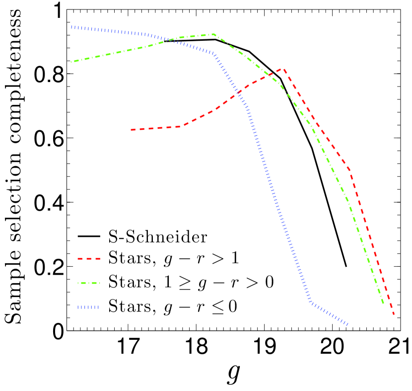
Figure 1: The clean PM sample selection completeness (defined as the ratio of the number of objects which survive our clean PM cut over the total number of objects) as a function of $g$-band magnitude for S-Schneider and all spectroscopic stars in SDSS DR7 (binned into three color bins).

where match is the number of objects in USNO-B which matches a SDSS object within a 1 arcsec radius, sigRa and sigDec are the rms residuals for the proper motion fit in right ascension and declination, nFit is the number of detections used in the fit including the SDSS detection (so nFit = 6 requires that the object was detected on all five USNO-B plates plus one for SDSS), and dist22 is the distance to the nearest neighbor in SDSS with $g<22$. We rejected PM entries which violate any of the above conditions. Specifically, for our main quasar sample S-Schneider (see below), the fraction of objects which violates each cut condition is: $8.2\%$ for nFit=4 (the minimum nFit in Munn et al. catalog), $17.3\%$ for nFit=5, $0.5\%$ for match $\neq$ 1, $2.9\%$ for sigRa $\geq$ 525 or sigDec $\geq$ 525 , and $5.6\%$ for dist22 $\leq$ 7. The sample selection completeness (defined as the ratio of the number of objects which survive the cut over the total number of objects) as a function of the $g$-band magnitude (the six $g$ bins in Table 1) for S-Schneider is shown in Figure 1. The selection completeness saturates at the bright end ($\sim 90\%$), and drops rapidly with decreasing magnitude. The selection completeness curves for several samples of stars are shown in the same plot for comparison. We pick out all spectroscopic stars in SDSS DR7, bin them into three color bins ($g-r>1.0,1.0\geq g-r>0,g-r\leq 0$), and carry out the same cleaning process to obtain the selection completeness as a function of $g$. As the color becomes redder the completenes for stars deceases at the bright end while increases at the faint end.

We note here that the way in which we trim the catalog for clean PM is different from the widely used standard procedure (e.g. Bond et al. 2010) which is recommended in the original sample design (Munn et al., 2004), where it only requires match = 1 and sigRa < 350 && sigDec < 350. Considerations of various selection criteria show that the standard PM selection criteria return a much less clean quasar PM distribution, which has significantly more quasars with spurious large PM values. Specifically, the important new condition nFit = 6 makes the cleanness of our samples much better than that of samples defined using the standard criteria defined by Munn et al. (2004), even when we loosen the requirement on rms fitting residuals a little bit (see Table 1 and discussion below). We would like to stress that the functional forms which we derive later in this paper for the PM error distribution can only be applied to clean PM samples as defined above.

We now use the several SDSS quasar catalogues from the literature to define samples for the analysis of the PM error distribution. Richards et al. (2009) selected $\sim 1.2$ million photometric quasar candidates from SDSS DR6 based on a Bayesian selection method employing the kernel density estimate (KDE) of the probability density function. The $i$ magnitude range for this sample is $\sim 17-21$. After selecting all the objects which passed their selection criterion, Richards et al. (2009) flagged the most likely contaminants by assigning a good index to every object. This index starts at 0 for each object, then is incremented or decremented based on a set of rules. In the end, every object is assigned a good index in the range of [-6,6], with larger positive values meaning a larger likelihood of being a quasar. For our purpose, we back out the part of the good index determination which makes use of the PM, and assign each object a new good^′ index which does not contain any PM information. We then choose objects with the new good^′ $\geq 3$ so that we obtain a clean sample (hereinafter S-Richards) while retaining enough objects to carry out the analysis.

Bovy et al. (2011) generated a SDSS quasar targeting catalog by assigning a probability as a star, low-redshift ($z<2.2$), medium-redshift, or high-redshift ($z>3.5$) quasar for $\sim 160$ million point sources with dereddened $i$-band magnitude between 17.75 and 22.45 in SDSS DR8. They did this by modeling the distributions of stars and quasars in flux space down to the SDSS flux limit by applying the extreme-deconvolution method to estimate the underlying density of each class as a function of magnitude, and then convolved the densities with the flux uncertainties to assign to each object the probability of its being a quasar. We select a subsample (here after S-Bovy) with available clean PM, and reject objects with good!=0 (objects fail on some of the $BOSS$ flag cuts), Photometric=0 (objects were observed under bad imaging condition) and quasar probability $\leq 99\%$ for all three categories.

Bond et al. (2010) selected 69,916 spectroscopic quasars from SDSS DR7 with $14.5<r<20$ and $0.5<z<2.5$. We repeat the selection to define the sample S-Bond using the above improved criteria for finding clean PM.

Schneider et al. (2010) produced the spectroscopic quasar catalog for SDSS DR7, which contains 105,783 spectroscopically confirmed quasars with luminosities larger than $M_{i}=-22.0$. This catalog has been visually inspected, has highly reliable redshifts from 0.065 to 5.46, and contains quasars fainter than $i\approx 15$. We select objects with clean PM from their catalog to form the sample S-Schneider. Again, we expect a large overlapping between S-Schneider and S-bond. Furthermore, to show the differences on the resulting samples due to different clean PM conditions, we select an additional sample S-Schneider-W from the Schneider quasar catalog with the recommended clean PM conditions in Munn et al. (2004) (match = 1 and sigRa < 350 && sigDec < 350).

Note that in all these samples, an object can have a large measured proper motion for two reasons. First, it could in fact has a real large proper motion, and is therefore presumably not, in fact, a quasar but a white dwarf or other peculiar star. These sneak through even in the spectroscopic samples (as an example, the object plate=1642, mjd=53115, fiber=81 is included in S-Schneider, but actually it is a white dwarf). Second, the proper motion measurement has occasionally failed for some reason, such as mismatches with USNO-B or bad deblends. Clearly the assignment of a proper motion error to the latter category or to the ‘tail’ of the main distribution is a bit subjective, but in fact for our samples is pretty clear, as we shall see.

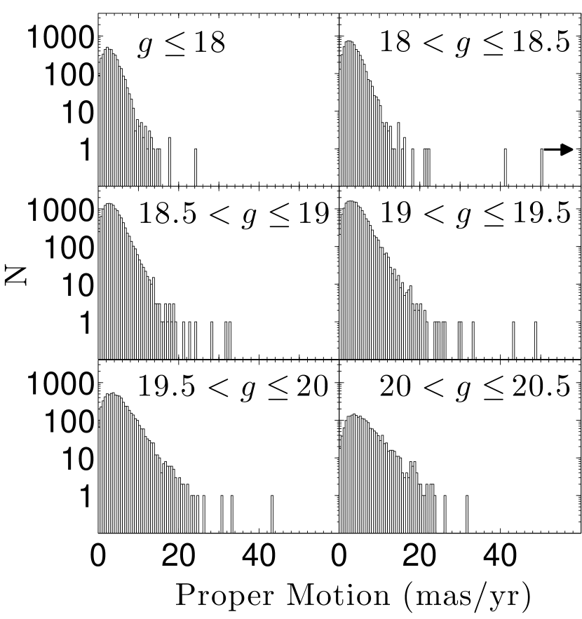
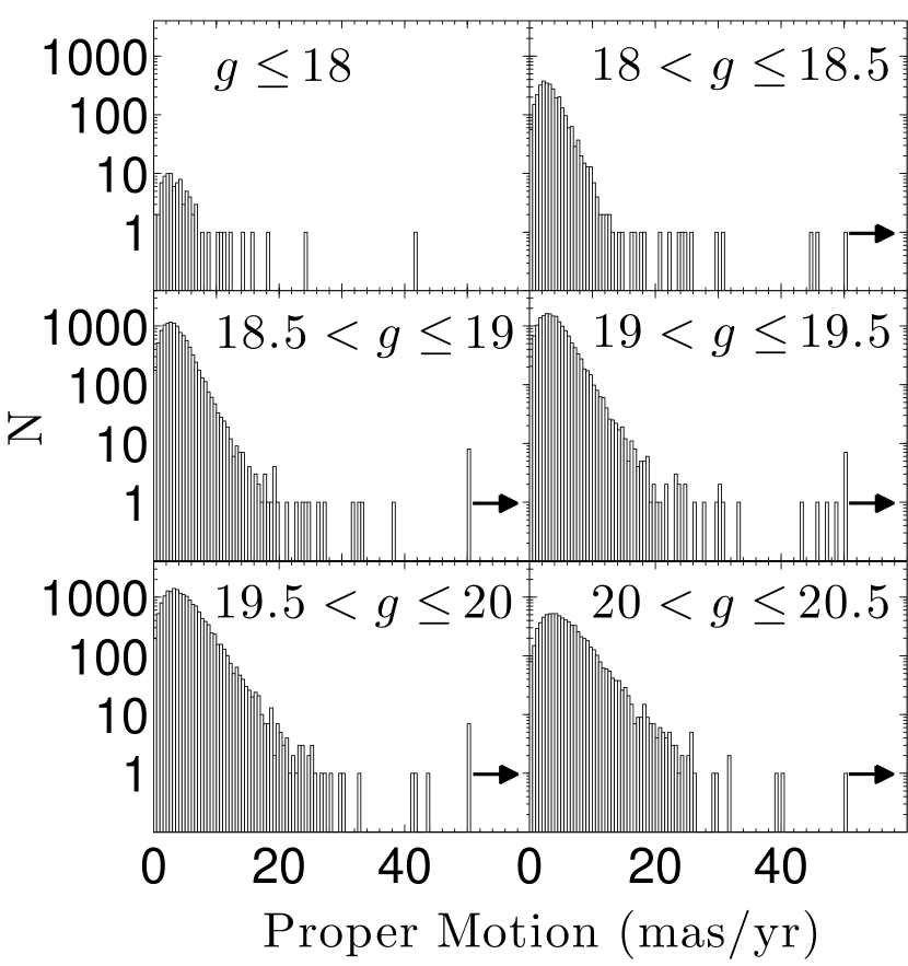
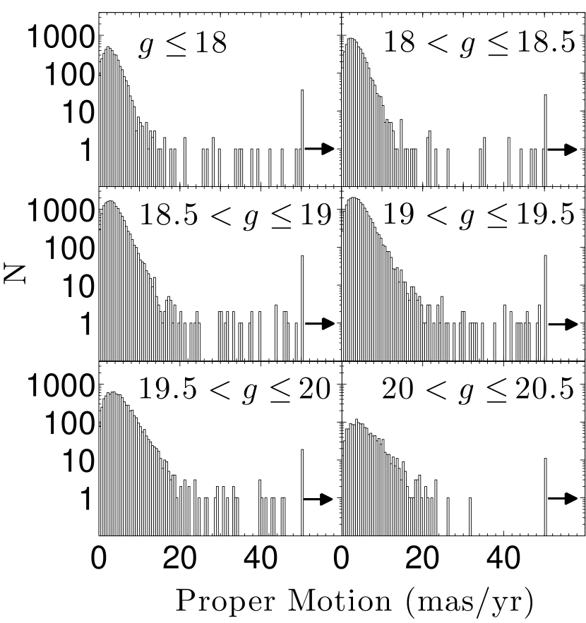
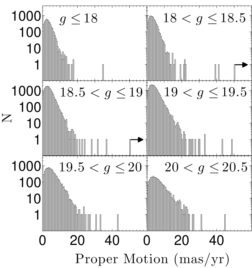
Figure 2: The PM distribution for S-Richards (upper left), S-Bovy (upper right), S-Bond (lower left), and S-Schneider (lower right), in six bins of $g$ magnitude (uncorrected for extinction). The arrows indicate that the last bin contains all the ${\rm PM}\geq 50$ mas yr^-1 objects.

The total PM (${\rm PM}=\sqrt[]{{\tt pml}^{2}+{\tt pmb}^{2}}$, where pml and pmb are the longitudinal and latitudinal components of PM in the Munn et al. catalog, where pml contains the factor of $\cos{b}$) distributions at 6 $g$-band bins for the four samples cuter by our strict clean PM criteria are shown in Figure 2, where the magnitude is the $psf$ magnitude without extinction correction. The statistical information for all the five samples is listed in Table 1, including the number of objects with PM$\geq 10$ mas yr^-1(the commonly assumed 3$\sigma$ uncertainty), and PM$\geq 30$ mas yr^-1(defined as the “outliers”, see below). We note that comparing with S-Schneider, S-Schneider-W is about $25\%$ larger in size, but contains over an order of magnitude more objects with PM$\geq 30$ mas yr^-1. These objects, which lie in the tail of the distribution, are almost certainly due to either contamination or failed PM measurement, as discussed above. Given the high quality of the eyeball-inspected Schneider catalog, very likely it is the latter which makes the most contribution. Again, in order to excluding these failed PM measurements as likely as possible, a strict set of clean PM conditions as ours should be applied instead of the original recommended one in Munn et al. (2004).

Among the four samples resulting from our good PM criteria, in general S-Richards (slightly better) and S-Schneider are the two cleanest, with fewer than $0.03\%$ of the objects having PM $>30$ mas yr^-1. That is as expected, since the spectra in the S-Schneider sample have been visually inspected and verified to have quasar-like spectra, and the high good^′ index objects in S-Richards have been cross matched with a lot of quasar-related information. In fact, in the magnitude range covered in this study, the samples overlap almost completely. On the other hand, S-Bovy performs as well as the previous two samples except at the very high PM end, while S-Bond has a substantially larger fraction of contamination by spurious high proper motion values. This is due to the fact that its selection only relies on the catalog spectroscopic redshift, which occasionally produces a false measurement by the spectroscopic pipeline, while the S-Schneider sample spectra were visually examined. The size of the four samples cutted by our strict good PM conditions varies from 50,375 (S-Richards) to 66,658 (S-Schneider), while S-Bovy has too few objects at the bright end for statistical use. For our purpose of studying the PM error distribution, we choose S-Schneider as the main sample for analysis, and also study S-Richards for comparison.

Table 1: Sample statistics

Number of objects in each category	S-Richards	S-Bovy	S-Bond	S-Schneider	S-Schneider-W
$g\leq 18.0$	3962	89	3893	4833	5131
$18.0<g\leq 18.5$	6371	2994	7193	8061	8504
$18.5<g\leq 19.0$	13397	10785	16076	17465	18794
$19.0<g\leq 19.5$	17862	17252	22247	24012	27549
$19.5<g\leq 20.0$	6711	16741	7846	9221	13459
$20.0<g\leq 20.5$	2072	7604	1434	3066	10075
Total	50375	55465	58689	66658	83512
PM$\geq 10$ mas yr-1	1535	1900	2623	1980	4180
PM$\geq 30$ mas yr-1	12	49	296	17	227
PM$\geq 50$ mas yr-1	1	24	214	2	70

3 The distribution of quasar PM

In this Section, we fit the total PM distribution in each $g$ magnitude bin of our quasar samples by analytic expressions, and investigate the dependence of the fitting result on magnitude. We use the magnitude uncorrected for extinction, since the errors should depend only on the apparent brightness of the source.

Equation 1 gives the core + wing function that we use to fit the quasar PM distributions:

$$f(p|A,\sigma,B,\alpha,\beta,c)=A\frac{p}{\sigma^{2}}e^{-\frac{p^{2}}{2\sigma^{2}}}+Bp^{\alpha}e^{-(\frac{p}{c\sigma})^{\beta}}$$ (1)

We here and in what follows assume that the proper motion errors are isotropic; we will return to this assumption below. We use a 2D Gaussian function to model the central part of the distribution, where $p$ is the proper motion, $A$ is the amplitude of the Gaussian core, and $\sigma$ is the width. For the wing part of the distribution, we tried various fitting functions, eventually finding that the second term in Equation 1 provides an adequate fit. $B$ is the amplitude, $\alpha$ and $\beta$ are two indices, and $c$ is a constant. With values of both indices close to 1, this wing function decays exponentially at large PM, as suggested by Figure 2, and is well-behaved at small PM with little effect on the gaussian core. For all magnitude bins, we use PM in the range of $0-30$ mas yr^-1 for fitting. Extrapolation to larger proper motion values is well-behaved, though even in the cleanest samples the few objects at larger values have flattish distributions and are almost certainly either contaminants or failed measurements. Thus we can say little about the distribution beyond 30 mas yr^-1, except to quote maximum probabilities for whatever causes a measurement error this large or larger to occur under the assumption that all the outliers are due to measurement error, which may well be true for S-Schneider. The fractions of these outliers in each $g$ bin are listed in Table 2.

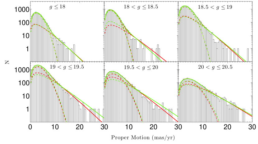
Figure 3: The fitting results for S-Schneider in six bins of $g$ magnitude (uncorrected for extinction). The red curves show the full six-parameter function (Equation 1), while the green curves show the two-parameter approximation ($\alpha=1.0,\beta=1.0,c=0.9$, Equation 1, and normalized $b=0.035$). The dash-dotted lines are the core of the distribution (first term in Equation 1 and 2), the dashed lines are the wing of the distribution (second term of Equation 1 and 2), and the solid lines are the combination of the two.

We minimize the total $\chi^{2}$ to fit the PM distribution at each bin to find $A,\sigma,B,\alpha,\beta$, and $c$. We then normalize the distribution function to get the probability function by replacing $A$ and $B$ with $a$ and $b$ to make the integral unity ($\int_{0}^{\infty}f(p|a,\sigma,b,\alpha,\beta,c)dp=1$). We plot the fitting results in Figure 3 for S-Schneider (red curves), and list the value of the parameters and the $\chi^{2}$ statistics in Table 2 for S-Schneider and S-Richards (first two sets of rows). The fits are generally good, with normalized $\chi^{2}$ in the range of 0.66-1.5 for both samples. The fitted parameters for the two samples are similar to each other, which indicates the robustness of the fitting function. (But remember that the two samples are not by any means independent.)

Table 2: Fitting parameters and statistics

Sample	$g$ range	$g_{ave}$	$f_{o}$	$a$	$\sigma$	$b$	$\alpha$	$\beta$	$c$	$\chi^{2}$	Normalized $\chi^{2}$
S-Richards	$g\leq 18.0$	17.52	0.000%	0.92	2.48	0.020	0.51	0.88	0.97	43.2	0.80
	$18.0<g\leq 18.5$	18.28	0.031%	0.88	2.53	0.016	1.03	1.03	0.93	59.7	1.11
	$18.5<g\leq 19.0$	18.78	0.015%	0.78	2.72	0.038	0.89	1.03	1.01	67.5	1.25
	$19.0<g\leq 19.5$	19.24	0.022%	0.71	2.99	0.036	1.10	1.06	1.06	80.9	1.50
	$19.5<g\leq 20.0$	19.70	0.045%	0.57	3.50	0.054	1.01	1.00	1.25	45.9	0.85
	$20.0<g\leq 20.5$	20.19	0.048%	0.46	3.76	0.039	1.11	1.01	1.10	40.8	0.76
S-Schneider	$g\leq 18.0$	17.53	0.021%	0.83	2.44	0.041	0.77	1.01	0.98	39.4	0.73
	$18.0<g\leq 18.5$	18.28	0.037%	0.89	2.53	0.016	1.00	1.01	1.06	68.3	1.27
	$18.5<g\leq 19.0$	18.78	0.017%	0.77	2.70	0.037	0.93	1.05	1.00	81.1	1.50
	$19.0<g\leq 19.5$	19.24	0.021%	0.67	2.98	0.044	1.14	1.04	0.86	74.6	1.38
	$19.5<g\leq 20.0$	19.70	0.033%	0.56	3.38	0.053	1.14	1.01	0.78	62.3	1.15
	$20.0<g\leq 20.5$	20.20	0.065%	0.52	3.80	0.036	1.14	1.00	0.86	35.4	0.66
S-Schneider	$g\leq 18.0$	17.53	0.021%	0.83	2.42	0.035	1.00	1.00	0.90	40.9	0.71
	$18.0<g\leq 18.5$	18.28	0.037%	0.82	2.51	0.035	1.00	1.00	0.90	74.9	1.29
	$18.5<g\leq 19.0$	18.78	0.017%	0.79	2.70	0.035	1.00	1.00	0.90	81.7	1.41
	$19.0<g\leq 19.5$	19.24	0.021%	0.74	3.01	0.035	1.00	1.00	0.90	93.4	1.61
	$19.5<g\leq 20.0$	19.70	0.033%	0.68	3.38	0.035	1.00	1.00	0.90	79.4	1.37
	$20.0<g\leq 20.5$	20.20	0.065%	0.57	3.91	0.035	1.00	1.00	0.90	38.6	0.67
S-Schneider-W	$g\leq 18.0$	17.53	0.12%	0.76	2.44	0.056	0.99	1.05	0.90	41.5	0.77
	$18.0<g\leq 18.5$	18.28	0.15%	0.85	2.53	0.022	1.05	1.04	1.03	55.2	1.02
	$18.5<g\leq 19.0$	18.78	0.13%	0.78	2.75	0.038	0.89	1.01	0.94	84.9	1.57
	$19.0<g\leq 19.5$	19.24	0.18%	0.75	3.08	0.034	0.97	1.00	0.90	134.3	2.49
	$19.5<g\leq 20.0$	19.72	0.35%	0.67	3.49	0.031	0.99	0.99	0.93	110.7	2.05
	$20.0<g\leq 20.5$	20.24	0.87%	0.46	4.18	0.033	1.12	1.00	0.88	71.6	1.33

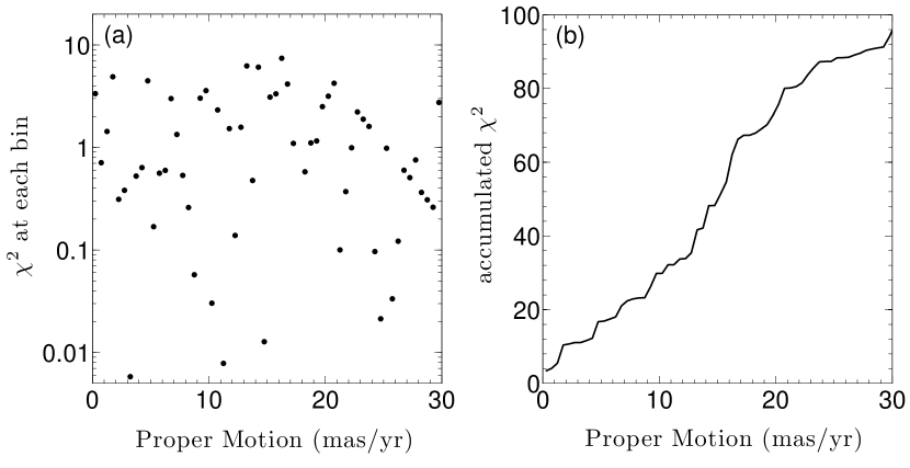
Figure 4: (a): The $\chi^{2}$ at each PM bin for the freedom reduced fitting for the $18<g\leq 18.5$ bin in S-Schneider. (b): the accumulated $\chi^{2}$ in this case (the degree of freedom is 58).

It is clear that several of the parameters do not change very much with magnitude, so we also conducted experiments in which we freeze the values of some of these, and refit the distributions with this reduced freedom. The third set of rows in Table 2 shows the best result from this exercise, where we fix $\alpha=1.0,~{}\beta=1.0,~{}c=0.9$, define a normalized tail amplitude $b=0.035$ (and a corresponding normalized gaussian amplitude $a=1-b(c\sigma)^{2}$). This makes the normalized probability function a one-parameter function of $\sigma$ alone; ($\int_{0}^{\infty}f(p|\sigma)dp=1$). Figure 3 shows these results (green curves), where it is clear that the difference between the full-freedom and the reduced-freedom fitting is small in all the magnitude bins. The total $\chi^{2}$ only moderately increases with the new fitting function (the normalized $\chi^{2}$ even drops in some cases due to an increase in the degree of freedom), and the largest increase occurs at the $19.0<g\leq 19.5$ magnitude bin (which also has the largest normalized $\chi^{2}$ (1.61) and the largest population, so is most sensitive to small inadequacies in the fitting function). We show the detailed $\chi^{2}$ map for this case in Figure 4. The $\chi^{2}$ at each PM bin are uniformly scattered around 1, and the accumulated $\chi^{2}$ behaves well. The normalized one-parameter fitting function is:

$$f(p|\sigma)=(1-0.035(0.9\sigma)^{2})\frac{p}{\sigma^{2}}e^{-\frac{p^{2}}{2\sigma^{2}}}+0.035pe^{-(\frac{p}{0.9\sigma})}$$ (2)

Due to the limited quasar sample size we can only fit its PM distribution and extract the fitted parameters at six $g$ magnitude bins (the average magnitude of each $g$ bin for both S-Schneider and S-Richards are listed in Table 2). To get the distribution function at some arbitrary $g$, we fit a quadratic function to the $\sigma$ in the fitting using the one-parameter fits (Equation 2, the only free parameter in the normalized function) as a function of $g$:

$$\sigma=0.2293(g-19)^{2}+0.6205(g-19)+2.836$$ (3)

Figure 5 shows the fitting results, which are very good. Bond et al. (2010) studied the PM error distribution using their quasar sample. They fitted a Gaussian profile to the error distribution in the entire magnitude range, and obtained a fitting function for $\sigma$, which is shown here as well for comparison (They fitted $\sigma$ as a function of $r$-band magnitude. To make a direct comparison we convert $r$ into $g$ via $g-r=0.18$, which is the average value for S-Schneider, see below.). In general, their fitted $\sigma$ is larger (by $\sim 0.5$ mas yr^-1) than ours in the entire magnitude range, while the two curves share very similar shapes. This is fully consistent with the fact that Bond et al. (2010) used a less clean quasar sample than S-Schneider and didn’t separate the tail of the distribution from the Gaussian core, both resulting in a larger Gaussian width. Our fitting formula, of course, applies only to a finite range in g magnitude, since we have only a finite range over which to determine it. We recommend using it in the range of $17.5\leq g\leq 20.5$ (the range we plot in the figure). For $g<17.5$ we recommend using a constant $\sigma=2.42$, because for bright objects the proper-motion measurement error approaches the instrument induced error limit and does not depend on the brightness of the object. For $g>20.5$, the fitting function is ill-constrained; we have too few quasars to calibrate it, and the core parameters are not well-determined.

Finally, we fit the fraction of the outliers ($f_{0}$ in Table 2) in S-Schneider as a function of $g$ magnitude. Given the small number of outliers (17), this fitting can only indicate the general trend of the $f_{o}-g$ relation. We approximate the fitting function by:

$$f_{o}=0.00122(10^{1.27(g-19)}+20.1)\%$$ (4)

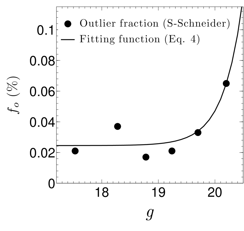
Figure 6: The fitted outlier fraction $f_{o}$ (Table 2) in S-Schneider as a function of $g$ (Equation 4).

(Note $f_{o}$ is in unit of $\%$.), and the fitting is shown in Figure 6. As is the case with the fitted $\sigma-g$ relation, we recommend confining the use of this relation to $g\lesssim 20.5$ since we have insufficient numbers of objects at fainter magnitudes. The extension to the brighter magnitudes can probably be trusted, however.

Before we move to the next section, there are several general issues about the PM error distribution that we would like to discuss.

1. Since most previous studies which used the SDSS+USNO-B PM catalog employed the original clean PM criteria in Munn et al. (2004) to select objects with good PM measurements, here we explore the effect of this weaker PM cut on the error distribution by fitting S-Schneider-W using Equation 1. The result is shown in Table 2 (bottom set of rows). Comparing with the fitting results of S-Schneider (the second set of rows in the same table), the original clean PM conditions results in a slightly larger $\sigma$ (up to $\sim 10\%$), and a generally worse $\chi^{2}$ statistics (both are more significant at the faint end). The biggest disadvantage of the original clean PM criteria is still, as we discussed above, that it introduces a much larger $f_{o}$. Studies of stellar kinematics which are sensitive to the outlier fractions, such as searching for extremely high velocity stars in the Galaxy, will be severely affected if this weaker set of clean PM criteria is applied instead of ours.

2. In principle, PM errors could depend on color as well as magnitude; Bond et al. (2010) found that the systematic errors in PM have a small color dependence, but did not find a corresponding dependence for the random errors. Basically, the color range of quasars is too small to investigate this possibility. Several color distributions for S-Schneider are shown in Figure 7. Stars, on the other hand, have a much wider range of colors and their measured proper motions may be subject to color-related errors which cannot be investigated with quasar samples. If this is the case, the error functions derived here are more applicable to samples of blue stars, such as main-sequence-turnoff samples. The POSS positions which enter the proper motion calculation are inverse-variance weighted combinations of data from the O, J, E, F, and N plates and thus span a very large wavelength range, most of which is to the red of the effective wavelength of the SDSS $g$ band, but it is not clear exactly what the effective wavelength is. But we probably somewhat overestimate the errors for red objects, because they are brighter in most of the photographic bands than typical quasars with the same $g$ magnitude, i.e. our result is a conservative limit for red objects (which is reason that we choose to investigate the dependence of the PM error distribution on $g$ magnitude instead of on redder bands). The mean $g-r$ color in the figure is 0.18, which corresponds to middle-late F stars. The sample we are investigating which prompted this study is a SEGUE II sample of halo turnoff stars, for which the color match with the quasars is (entirely fortuitously) excellent.

3. There are additional possible contributions to the PM errors, such the way of measuring the position of the objects on the sky and observing conditions. The USNO-B positions are originally in the coordinate system of the USNO plates and then later transferred to the celestial coordinates (right ascension and declination), while the SDSS positions are initially measured in the CCD coordinate system, which later are transferred to the survey longitude and latitude which define the photometric scans of the sky, and are then calibrated with respect to the ra-dec measurements from UCAC. The derivation of proper motions from these two sets of measurements has the probable effect of making the errors in the proper motions more nearly isotropic (See point 3 below). Bond et al. (2010) looked at the dependence of median and rms errors for the longitudinal and latitudinal PM components on position on the sky, and concluded that the variation is relatively small (with the median variation being much smaller than $\sigma$). On the other hand, whether the PM error distribution (especially the wing component) depends systematically on position on the sky is another question, which again we are not able to address due to the limited size of the quasar samples. Note, however, that our investigation deals well with the aggregate survey, so questions like the number of outliers expected with samples large enough to sample the sky in a manner comparable to the quasars should be well answered.

4. We investigate the error distribution for the total PM and not for the individual components of the PM, since the errors are likely to be isotropic and, for many purposes, it is the total PM which matters. Bond et al. (2010) concluded that the correlation between the errors in the two components is negligible compared to the total random and systematic errors. In addition, we find that the error distributions in the two components are very similar, as shown in Figure 8. For S-Schneider, the median is $0.10$ for pml and $-0.17$ for pmb, both significantly smaller than the Gaussian width $\sigma$, and the standard deviation is 3.40 for pml and 3.43 for pmb. This inferred near-isotropy of the PM errors, however, should be viewed with some caution, as the l and b components are related in a very complex and variable way to components either along and perpendicular to the scan directions in SDSS, altitude and azimuth, or right ascension and declination, for which in any of those cases there might be factors contributing to anisotropy.

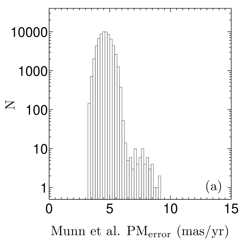
Figure 9: The distribution of the PM error estimate (${\rm PM}_{\rm error}=\sqrt{{\tt pmraerr}^{2}+{\tt pmdecerr}^{2}}$) in the Munn et al. catalog for S-Schneider.

5. In addition to providing the PM measurement, Munn et al. (2004) also provided a PM error estimate (pmraerr and pmdecerr, which represent the expected standard deviations of the PM measurement around the true value in each direction, but the two components are always assumed to be the same in the catalog). Since most previous investigations which used the SDSS stellar kinematics to study the galactic structure employed the catalog-provided pmraerr and pmdecerr to estimate the uncertainty of the PM measurement, it is worth calibrating the performance of this error estimate using the true PM error distribution which we get from our quasar samples. We calculate the total catalog-provided PM error estimate (${\rm PM}_{\rm error}=\sqrt{{\tt pmraerr}^{2}+{\tt pmdecerr}^{2}}$) for S-Schneider, and show its statistical distribution in Figure 9. The distribution is rather narrow, effectively ranging from $3-6$ mas yr^-1. In addition, we provide the average pmraerr (or pmdecerr) for each $g$ bin, and over plot it in Figure 5 (from small to large $g_{avg}$, the values are 2.78, 2.99, 3.18, 3.37, 3.54, and 3.69 mas yr^-1). We note here although we use a 2D Gaussian function to model the core part, the $\sigma$ in the PM error pdf is still a 1D Gaussian $\sigma$ (i.e. in one direction, assuming isotropy for the distribution), so it is pmraerr (or pmdecerr) which should be compared with the fitted $\sigma$, not ${\rm PM}_{\rm error}$. The comparison shows that the catalog-provided error estimate is in good agreement with our fitted $\sigma$ (within $20\%$), with the former on average being $\sim 12\%$ higher than the latter (the agreement is better at the faint end). The major drawback of the catalog-provided error estimate is that it does not address the non-Gaussian tail of the error distribution. In the further, we recommend that analysis using the Munn et al. PM, especially the ones for which the tale of the PM error distribution is important, should use our results to estimate the error instead of using the catalog-provided errors.

4 The Significance of the measured proper motions

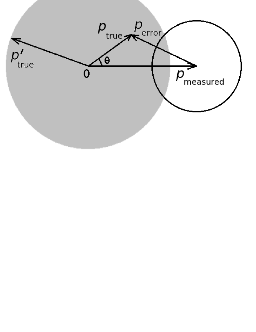
Figure 10: Schematic plot which shows how we calculate the probability $F(p_{\rm true}\leq p_{\rm true}^{\prime})$.

With the normalized PM distribution function $f(p)$ for our quasar samples, we can calculate the PM error probability function ($f(p_{\rm error})=f(p)$) of the measured PM ($p_{\rm measured}$) for an object (a star) with intrinsic non-zero PM. Specifically, $f(p_{\rm error})dp_{\rm error}$ is the probability that the true proper-motion $\vec{p}_{\rm true}=\vec{p}_{\rm measured}+\vec{p}_{\rm error}$ falls in an annulus centered on $\vec{p}_{\rm measured}$ with radius $p_{\rm error}$ and $p_{\rm error}+dp_{\rm error}$. (see Figure 10). Based on this, we could calculate the probability of an object with $\vec{p}_{\rm measured}$ having an (unknown) true PM $p_{\rm true}$ larger than some certain value $p_{\rm true}^{\prime}$. As shown in Figure 10, the total probability of $p_{\rm true}$ being in the shadowed area ($p_{\rm true}\leq p_{\rm true}^{\prime}$) is:

$$F(p_{\rm true}\leq p_{\rm true}^{\prime})=\int_{0}^{p_{\rm true}^{\prime}}\frac{f(p_{\rm error})}{2\pi p_{\rm error}}pdpd\theta$$ (5)

While $\vec{p}_{\rm error}=\vec{p}_{\rm true}-\vec{p}_{\rm measured}$ so $p_{\rm error}=\sqrt[]{p_{\rm measured}^{2}+p_{\rm true}^{2}-2p_{\rm measured}p_{\rm true}\cos{\theta}}$. The above integral turns into:

$$F(p_{\rm true}\leq p_{\rm true}^{\prime})=\int_{0}^{p_{\rm true}^{\prime}}\frac{f(\sqrt[]{p_{\rm measured}^{2}+p^{2}-2p_{\rm measured}p\cos{\theta}})}{2\pi\sqrt[]{p_{\rm measured}^{2}+p^{2}-2p_{\rm measured}p\cos{\theta}}}pdpd\theta$$ (6)

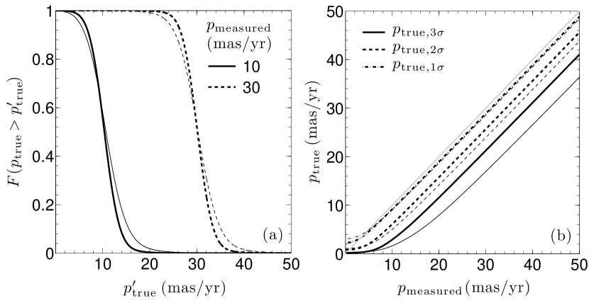
Figure 11: (a): The calculated probability $F(p_{\rm true}>p_{\rm true}^{\prime})$ (Section 4) as a function of $p_{\rm true}^{\prime}$ for two measured PM at 10 and 30 mas yr^-1. (b): Three confidence levels for the true PM (Section 4) as a function of measured PM. In both plots thick lines are for $g=18.28$, and thin lines are for $g=19.70$. Here 1, 2, and 3 $\sigma$ refer to probabilities of 68%, 95%, and 99.7% that the true PM exceeds the plotted value.

Thus $F(p_{\rm true}>p_{\rm true}^{\prime})=1-F(p_{\rm true}\leq p_{\rm true}^{\prime})$ is the probability that $p_{\rm true}$ falls outside the shadowed area, i.e. the object in consideration has a true PM larger than the given threshold $p_{\rm true}^{\prime}$. Panel $(a)$ in Figure 11 shows the calculation of $F(p_{\rm true}>p_{\rm true}^{\prime})$ for two measured PM at two $g$ magnitudes ($18.28$ and $19.70$). Based on this, we define a series of confidence intervals ($p_{\rm true,1\sigma}$, $p_{\rm true,2\sigma}$, and $p_{\rm true,3\sigma}$) to be the $p_{\rm true}^{\prime}$ corresponding to $F(p_{\rm true}>p_{\rm true}^{\prime})=68\%$, $95\%$, and $99.7\%$. Panel $(b)$ in Figure 11 shows these confidence intervals.

Here we use an example to illustrate the effect of the non-Gaussian tail in the PM error distribution in determining the confident velocity of a star with some measured PM. For a star with measured PM of 30 mas yr^-1 (corresponding to a transverse velocity of 423 km s^-1 at a helio-centric distance of 3 kpc) and $\sigma$ of 4 mas yr^-1, if the PM error distribution only contains the Gaussian core (e.g. $f(p|\sigma)=(p/\sigma^{2})e^{-p^{2}/(2\sigma^{2})}$), the $2\sigma$ confident PM would be 23.7 mas yr^-1(334 km s^-1) and the $3\sigma$ PM$=19.3$ (272 km s^-1). On the other hand, when including the non-Gaussian tail, the 2$\sigma$ and 3$\sigma$ confident PM decrease to 22.6 and 13.8 mas yr^-1(319 and 195 km s^-1. When combining with a model of the Galactic potential and a radial velocity, these differences in confident velocity may flip the conclusion that whether this star is bonded to the Galaxy or not. In general, the effect of the non-Gaussian tail is more prominent at the faint end, where the Gaussian width is larger and the weight of the non-gaussian tail is bigger.

Lastly, we note that in this section all the calculations are done with the one-parameter error probability function $f(p_{\rm error})=f(p|\sigma(g))$ (Equation 2 and Table 2), but it is a trivial exercise to replace $f(p|\sigma)$ with $f(p|a,\sigma,b,\alpha,\beta,c)$ (Table 2) if more accurate results are desired. However, in doing so one needs to interpolate the parameters at the six discrete $g$ magnitudes to get the result at some arbitrary $g$.

5 Summary and discussion

We have investigated the proper-motion measurement errors in the SDSS+USNO-B proper-motion catalog (Munn et al., 2004) by analyzing the proper-motion distributions of several recent SDSS quasar samples (Richards et al., 2009; Bond et al., 2010; Schneider et al., 2010; Bovy et al., 2011). The sample defined by Schneider et al. (2010)was determined to be the cleanest sample and has the largest sample size. We bin the data into six $g$ magnitude (not extinction corrected) bins, and fit analytic functions for the PM distribution in each bin. We find that, while a six-parameter fitting formula (Equation 1) describes the quasar PM distribution well, a simpler (normalized) function with one free parameter (Equation 2) also gives reasonably good results. Based on this fitting function for the PM error distribution, we calculate the probability that an object with a measured PM has a true PM $p_{\rm true}$ larger than a given threshold $p_{\rm true}^{\prime}$. Cutting the probability $F(p_{\rm true}>p_{\rm true}^{\prime})$ at several confidence levels, we calculate the “most likely PM” for a given measured PM.

The analysis raised several issues which we would like to stress:

1. Our PM error analysis can only be applied to clean PM subsamples from the SDSS+USNO-B catalog, which satisfies our strict clean PM criteria (match = 1, sigRa < 525 && sigDec < 525, dist22 > 7, and most importantly, nFit = 6, which requires that the object was detected on all five USNO-B plates). Experiments show that weakening this set of conditions (specifically, the original criteria in Munn et al. (2004): match = 1 and sigRa < 350 && sigDec < 350) generally results in a broader Gaussian core width (up to $10\%$), a worse $\chi^{2}$ statistics in the fitting, and a significantly higher fraction of the outliers (by an order of magnitude). Studies which are sensitive to the tail of the PM error distribution and the fraction of outliers, such as searching for extremely high velocity stars in the Galaxy, will be severely affected if using this weaker set of conditions instead of ours.

2. The PM error distribution derived here applies to $g$ magnitudes (without extinction correction) in the range $\sim 17-20.5$. Specifically, the fitting functions Equation 2 and 3 are only good for $17.5\leq g\leq 20.5$. Though using a constant $\sigma$ for brighter objects is probably appropriate, using a constant or extrapolating our results for fainter magnitudes is not (Section 3).

3. While we have derived a fitting function for the entire PM error range, we note that there is a small fraction of “outliers” (defined here to be PM error $>30$ mas yr^-1), which apparently do not belong to the derived error distribution. Even for our cleanest quasar sample, which has passed spectroscopic visual inspection (Schneider et al., 2010), and with our very conservative PM culling conditions, there is still a small number of outliers, up to $\sim 0.1\%$, in the faintest magnitude bands. We do not speculate on the origin of these, but they are likely present in any sample chosen by our criteria.

4. While we fit the PM error distribution as a function of magnitude, the readers should bear in mind that the PM error may depend on other parameters as well, such as color and position of the objects on they sky. The PM error distribution in this work is best applicable to objects in the color range similar to the quasar sample we use to get the distribution (i.e., blue stars, Fig. 7), though our result could be considered as a conservative limit for redder objects. While the median and rms for the PM error only weakly depend on the position on the sky, we do not have a large enough sample to investigate the dependence of the distribution on the position on the sky. The distributions of the PM error components in the longitudinal and latitudinal are very similar to each other (Fig. 8), and the correlation between the two is negligible compared to the total random and systematic errors.

5. Last, we note that the PM error estimate provided by Munn et al. (2004, pmraerr and pmdecerr) is in rough agreement with the $\sigma$ fitted from the quasar PM distribution (Fig. 5). The agreement is within $20\%$, and better at the faint end. On the other hand, the major drawback of the catalog-provided error estimate is that it does not address the non-Gaussian tail. We recommend that future analysis using Munn et al. proper motions, especially the ones for which the tail of the error distribution is important, should use this work to estimate the error instead of using the catalog-provided error estimate.

This investigation of the PM error are useful in many ways. For example, we are studying the kinematics of stars in SEGUE II, focusing on these hyper velocity ones with velocity exceeding the escape velocity of the Galactic potential. In this case, it is crucial to have an accurate PM error distribution to judge the significance of the hyper velocity for these escapers.

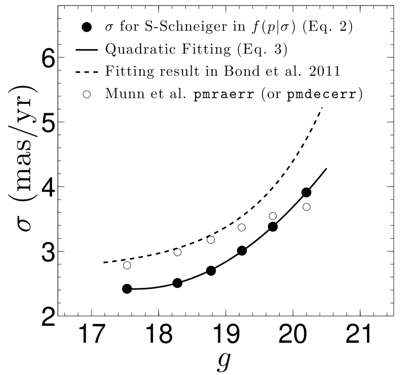
Figure 5: The value of $\sigma$ in the approximate distribution (Equation 2) of the quasar PM in S-Schneider as a function of average $g$ magnitude (solid point, the third set of rows in Table 2), and the corresponding fitting function (solid line, Equation 3). The dashed line shows the $\sigma$ fitting result in Bond et al. (2010) (their Equation 1. We convert the $r$ magnitude into $g$ magnitude by $g-r=0.18$, the average value for S-Schneider.). The open circles are the average catalog-provided PM error estimate in Munn et al. catalog (pmraerr or pmdecerr) for each $g$ bin.

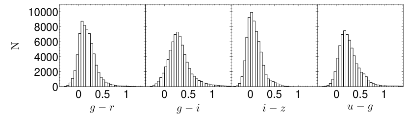
Figure 7: Histograms of colors (no extinction correction) for S-Schneider.

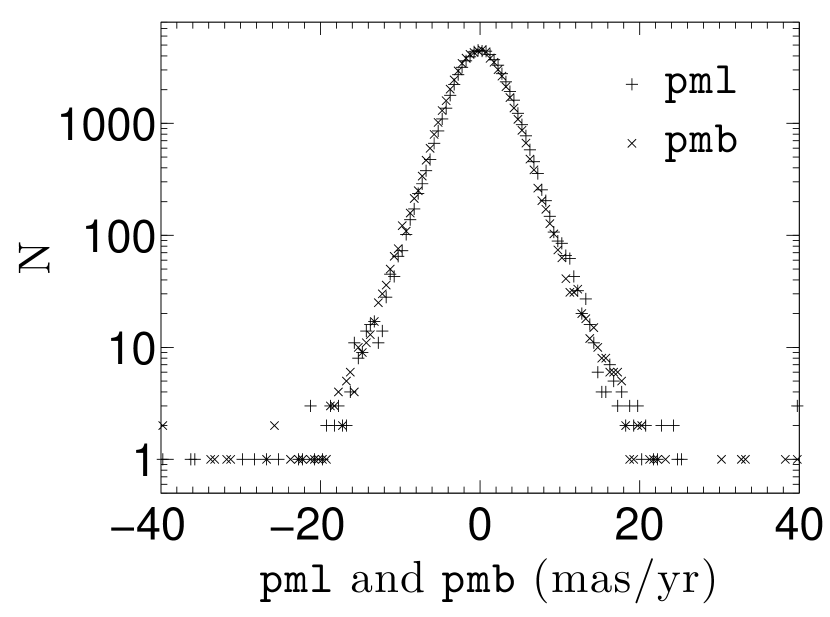
Figure 8: The distribution of PM in each component (pml and pmb) in the Munn et al. catalog for S-Schneider.

References

- SDSS-III collaboration: Aihara et al. (2011) SDSS-III collaboration: Aihara, H., et al. 2011, ApJS, 193, 29
- Bramich et al. (2008) Bramich, D. M., et al. 2008, MNRAS, 386, 887
- Bond et al. (2010) Bond, N. A., et al. 2010, ApJ, 716, 1
- Bovy et al. (2011) Bovy, J., et al. 2011, ApJ, 729, 141
- Carollo et al. (2010) Carollo, D., et al. 2010, ApJ, 712, 692
- Fuchs et al. (2009) Fuchs, B., et al. 2009, AJ, 137, 4149
- Gould & Salim (2003) Gould, A., & Salim, S. 2003, ApJ, 582, 1001
- Gunn et al. (1998) Gunn, J. E., et al. 1998, AJ, 116, 3040
- Kilic et al. (2006) Kilic, M., et al. 2006, AJ, 131, 582
- Lépine & Scholz (2008) Lépine, S., & Scholz, R.-D. 2008, ApJ, 681, L33
- Lupton et al. (2001) Lupton, R., Gunn, J. E., Ivezić, Ž., Knapp, G. R., & Kent, S. 2001, Astronomical Data Analysis Software and Systems X, 238, 269
- Majewski (1992) Majewski, S. R. 1992, ApJS, 78, 87
- Monet et al. (2003) Monet, D. G., et al. 2003, AJ, 125, 984
- Munn et al. (2004) Munn, J. A., et al. 2004, AJ, 127, 3034
- Munn et al. (2008) Munn, J. A., et al. 2008, AJ, 136, 895
- Richards et al. (2009) Richards, G. T., et al. 2009, ApJS, 180, 67
- Salim & Gould (2003) Salim, S., & Gould, A. 2003, ApJ, 582, 1011
- Sesar et al. (2008) Sesar, B., Ivezić, Ž., & Jurić, M. 2008, ApJ, 689, 1244
- Schlaufman et al. (2009) Schlaufman, K. C., et al. 2009, ApJ, 703, 2177
- Schneider et al. (2002) Schneider, D. P., et al. 2002, AJ, 123, 567
- Schneider et al. (2010) Schneider, D. P., et al. 2010, AJ, 139, 2360
- Smith et al. (2009) Smith, M. C., et al. 2009, MNRAS, 399, 1223
- Stoughton et al. (2002) Stoughton, C., et al. 2002, AJ, 123, 485
- Yanny et al. (2009) Yanny, B., et al. 2009, AJ, 137, 4377
- York et al. (2000) York, D. G., et al. 2000, AJ, 120, 1579
- York et al. (2000) York, D. G., et al. 2000, AJ, 120, 1579
- Zacharias et al. (2010) Zacharias, N., et al. 2010, AJ, 139, 2184