On the Scaling of Langevin and Molecular Dynamics Persistence Times of Non–Homogeneous Fluids.

Abstract

The existing solution for the Langevin equation of an anisotropic fluid allowed the evaluation of the position dependent perpendicular and parallel diffusion coefficients, using Molecular Dynamics data. However, the time scale of the Langevin Dynamics and Molecular Dynamics are different and an anzat for the persistence probability relaxation time was needed. Here we show how the solution for the average persistence probability obtained from the Smoluchowski-Fokker-Planck equation (SE), associated to the Langevin Dynamics, scales with the corresponding Molecular Dynamics quantity. Our SE perpendicular persistence time is evaluated in terms of simple integrals over the equilibrium local density. When properly scaled by the perpendicular diffusion coefficient, it gives a good match with that obtained from Molecular Dynamics.

I Introduction

The understanding of the dynamics of anisotropic fluids is fundamental in the study of many chemical and biophysical processes, particularly those occurring under nano-confinement. Molecular quantities like the mean square displacement (MSD), the mean first passage time (MFPT), and probability functions as the survival or persistence probability, can be readily obtained from a regular Molecular Dynamics (MD) simulation. However, phenomenological quantities are bounded to the equations and approximations that defined them. Thus, one commonly has to invoke some sort of approximation or condition for their validity. For instance, the diffusion constant is defined through the stochastic Langevin equation as a ratio of the approximate fluctuation force to the mechanical friction force in the so called Smoluchowski time scale. On a previous work clor , we presented an analytical solution for the Langevin equation of an anisotropic fluid, next to an attractive wall, which allowed the evaluation of the position dependent perpendicular diffusion coefficient. The mean squared displacement (MSD) and the average persistence time $\tau(z)$, needed to compute this coefficient, were obtained from a modification of the virtual layers molecular dynamics method (VLMD) of Liu et al.liu .

A serious difficulty found was that the time scale of the Langevin Dynamics and of the Molecular Dynamics did not match. In fact, it was discussed by Burschka et al. burska , Harris harris , and Razi Naqvi et al. razi , that the conditional probability obtained as the stationary solution of the Fokker–Planck equation, associated to the Langevin equation for a system with absorbing boundaries conditions fails to vanish at those boundaries. For the same space sampling layers width $L$, the Langevin persistence probability is then known to be lower than the corresponding MD persistence probability. That is, MD particles reach the boundary faster than Langevin particles. In another words, the Langevin dynamics (LD) average persistence time, $\tau_{{}_{LD}}$, for a given sampling layer width, is lower than the corresponding molecular dynamics time $\tau_{{}_{MD}}$. This is a systematic inconsistency, found even for virtual absorbing layers located at the bulk. It has been handled in the literature by shifting the boundaries away. In fact, Liu, Harder and Berne liu overcame this difficulty, by running simultaneous dual numerical LD and MD simulations, changing the value of $L$, until the survival probabilities from both simulations matched. Alternatively we appealed to the simplest ansatz of fixing the layer width and shifting the $\tau_{{}_{MD}}$ time instead clor .

In this paper we take a closer look at this problem, by solving the backwards Smoluchowski-Fokker-Planck equation (SE) associated to the anisotropic Langevin equation and comparing the resulting $\tau_{{}_{{\color[rgb]{0,0,0}SE}}}(z)$ with the $\tau_{{}_{MD}}(z)$ measured from the VLMD method. In the next section we briefly review the probability concepts in the VLMD method. After establishing the relation between the mean first passage time and the persistence time, we shall obtain an expression for the SE average persistence time. Finally in the last section, we shall discuss the scaling between the SE and MD dynamics, carrying out calculations for a simple Lennard-Jones dense fluid next to an attractive wall.

II Virtual Layer Molecular Dynamics Method

In this work we will use the VLMD method as discussed previouslyclor . It is a modification of the one introduced by Liu et al. (LHB) liu and Thomas et al. thomas . Briefly, once the dynamics is equilibrated, the total simulation time $s$ is divided in discrete time steps $\Delta s$ and partitioned in $J$ blocks containing $n_{max}$ time steps. The MD simulation time interval after n steps is then $t=n\Delta s$. The z coordinate perpendicular to the attractive walls is also divided in discrete virtual layers of width $L$. We then consider the set of particles that stay in a given layer located at $z_{a}$, i.e. $z(t)\in\{a,b\}=\{z_{a},z_{a}+L\}$, during the time interval $t$, spanning between the simulation time $s_{0}$ and $s=s_{0}+t$. The initial number of particles in the layer at $s=s_{0}$ is $N(0)=N(s_{0})$, and the number of particles in the set, still in the layer after the interval $t$, is $N(t)=N(s_{0}+t)$. The maximum time interval used to evaluate quantities inside the layers was $t_{max}=n_{max}\Delta s$. After $n_{max}$ steps the algorithm is re–initiated to measure the dynamics in the layer, setting $s_{0}=s$ again. This layer sampling is repeated $J$ times. We denote the number of particles in the set that stay in a layer in the $j^{th}$ layer sampling or repetition as $N_{j}(t)$.

In the VLMD method, the dynamical properties of the anisotropic fluid are evaluated layer by layer using absorbing boundary conditions. That is, particles that exit a given layer are not further counted, even if they reenter the region. The dynamics in the $z$ direction is governed by the behavior of $P(z,t;z_{{}_{0}})$, the joint probability of finding a particle at position $z_{{}_{0}}$ at time $t=0$ and then at position $z$ at time $t$. For an anisotropic system this function depends on the position where the layer is located, a$=z_{{}_{a}}$, and on the width $L$ of the space interval. The validity and accuracy of the VLMD method rely on the proper choice of Lclor ; liu . It was found that if L is too large the mean force within the layer changes more than required by the method. While, if it is too small, particles tend to escape from the virtual layer, affecting the proper statistics of the MD. For the fluid conditions used, L equal to 0.5 diameters was found to be a good compromise.

Since the movement in the $z$ direction is assumed to be independent of the movement in the $x$ and $y$ directions, the joint probability function is given as

$$P(z,t,z_{{}_{0}})=P(z,t|z_{{}_{0}})p_{a}(z_{{}_{0}}),$$ (1)

where $P(z,t|z_{{}_{0}})$ is the bayesian conditional probability that the particle is located at $z$ at time $t$, given that it was at $z_{{}_{0}}$ at time $t=0$, in a layer containing $z_{{}_{0}}$. $p_{a}(z_{{}_{0}})$ is the probability for a particle to be at position $z_{{}_{0}}$ at time $t=0$, normalized in the given region. It can be obtained directly from the local particle density $\rho(z)$.

$$p_{a}(z_{{}_{0}})=\frac{\rho(z_{{}_{0}})}{\int_{a}^{b}\rho(z)dz}.$$ (2)

The normalization of the joint probability is by definition the persistence probability, $\mathcal{P}(t,z_{a})$, in the diffusion domain $z_{a}\leq z<z_{a}+L$

$$\mathcal{P}(t,z_{a})=\int_{z_{a}}^{z_{a}+L}\!\!\!dz\int_{z_{a}}^{z_{a}+L}\!\!\!dz_{{}_{0}}P(z,t;z_{{}_{0}}).$$ (3)

It measures the average probability that after a time interval $t$ a particle still remains inside a layer located at $z_{a}$, independently of the initial position. $\mathcal{P}(t;z_{a})$ is often also called the survival probability liu , however, we prefer to call it the persistence probability to distinguish from the survival probability $G(t,z_{{}_{0}};z_{{}_{a}})$, as defined in the literature gardiner ; ColmenaresPRE

$$G(t,z_{{}_{0}};z_{{}_{a}})=\int_{a}^{b}P(z,t|z_{{}_{0}})dz.$$ (4)

$G(t,z_{{}_{0}};z_{{}_{a}})$ is the probability that at time $t$, the particle, initially located at $z_{{}_{0}}$, remains anywhere in the region $\{a,b\}$. So, while the survival probability is a function of the initial position, the persistence probability is independent of it.

In a MD simulation, the probability $\mathcal{P}(t,z_{a})$ is obtained by averaging $P_{j}(t)=N_{j}(t)/N_{j}(0)$ over the $J$ repetitions

$$\mathcal{P}(t,z_{a})=\frac{1}{J}\sum_{j=1}^{J}P_{j}(t).$$ (5)

As it has been shown by Molecular, Generalized Langevin and Langevin Dynamics $\mathcal{P}(t,z_{{}_{a}})$ can be phenomenologically approximated with a high degree of accuracy by an exponential decay liu ; thomas ; clor ,

$$\mathcal{P}(t,z_{{}_{a}})=e^{{}^{-t/\tau(z_{{}_{a}})}},$$ (6)

where $\tau(z_{{}_{a}})$ is the the relaxation time of the persistence process, also referred to as the average persistence time. The MD $\tau(z_{{}_{a}})$ is evaluated from Eq. (6), by fitting the numerical $\mathcal{P}(t,z_{{}_{a}})$ MD data.

All other physical properties of interest are evaluated as averages over the joint probability. For instance, the mean square displacement (MSD) in a layer is obtained as the average

$$\left\langle(z(t)-z_{{}_{0}})^{2}\right\rangle_{a}=\int_{z_{a}}^{z_{a}+L}\!\!\!dz\int_{z_{a}}^{z_{a}+L}\!\!\!dz_{{}_{0}}[z(t)-z_{{}_{0}}]^{{}^{2}}P(z,t,z_{{}_{0}}).$$ (7)

This expression also holds for the $x$ and $y$ directions. In the MD simulation the mean square displacement (MSD) within the layer at $a$ is evaluated summing over all the $N_{j}(t)$ particles in the set

$$\left\langle\left[z(t)-z(0)\right]^{2}\right\rangle_{a}=\frac{1}{J}\sum_{j}^{J}\frac{1}{P_{j}(t)}\left[\frac{1}{N_{j}(0)}\sum_{i}^{N_{j}(t)}\left[z_{i}(t)-z_{i}(0)\right]^{2}\right].$$ (8)

III Mean First Passage Time and Persistence Probability

In this section we will develop the relation between the MFPT and the mean survival time of particles dwelling in the layer. Using Eqs. (1) and (4), we rewrite Eq. (3) as an average over the initial position and find that a particle dwells in a given layer with a persistence probability

$$\mathcal{P}(t;z_{a}) = \int_{z_{a}}^{z_{a}+L}\!\!\!dz\left[\int_{z_{a}}^{z_{a}+L}\!\!\!dz_{{}_{0}}P(z,t|z_{{}_{0}})\right]p_{{}_{a}}(z_{{}_{0}}),$$ (9)

$$= \int_{a}^{b}dz_{{}_{0}}G(z_{{}_{0}},t)p_{{}_{a}}(z_{{}_{0}}).$$ (10)

In the context of this note, the average persistence time that the particles spend in motion within the virtual layer is then given, according to Eq. (6) by the integration of $\mathcal{P}(t,z_{{}_{a}})$ over the time interval. Using Eqs. (9) and (10) we get

$$\tau(z_{{}_{a}}) = \int_{0}^{\infty}dt\mathcal{P}(t,z_{{}_{a}}),$$ (11)

$$= \int_{a}^{b}dz_{{}_{0}}\left[\int_{0}^{\infty}dtG(z_{{}_{0}},t)\right]p_{{}_{a}}(z_{{}_{0}}),$$

$$= \int_{a}^{b}dz_{{}_{0}}[t_{{}_{MFP}}(z_{{}_{0}})]p_{{}_{a}}(z_{{}_{0}}),$$

where we have defined the mean time it takes a particle to reach the boundary given that it started at $z_{{}_{0}}$ as the mean first passage time $t_{{}_{MFP}}(z_{{}_{0}})$ (MFPT)gardiner

$$t_{{}_{MFP}}(z_{{}_{0}})=\int_{0}^{\infty}dtG(z_{{}_{0}},t).$$ (12)

Note that when the virtual boundaries of the layer are absorbing, the MFPT is actually a mean exit time. Thus, according to Eq. (11), $\tau(z_{{}_{a}})$ is simply the space average of $t_{{}_{MFP}}(z_{{}_{0}})$

$$\tau(z_{{}_{a}})=\langle t_{{}_{MFP}}(z_{{}_{a}})\rangle_{{}_{a}}.$$ (13)

The MFPT have the nice feature that they can be evaluated in terms of the equilibrium particle density. In earlier work, we have associated the MFPT with effective diffusion constants for confined ionic and non ionic fluids, and with local diffusion coefficients in anisotropic nano–confined molecular dense fluidsclor ; ColmenaresPRE ; SOVCLTheochem ; SulbaranCMP . So, in the next section we will obtain the expressions for the MFPT from the Smoluchowki-Fokker-Planck equation associated to the Langevin equation.

IV Langevin Dynamics Mean First Passage Time

The $z$ component of the anisotropic Langevin–like equation, can be written asliu ; clor

$$m\frac{d\mbox{v}(z)}{dt}=-\gamma_{{}_{zz}}\mbox{v}(z)+F(z)+\sigma(z)\,\xi(t).$$ (14)

It describes the dynamics of a fluid particle of mass $m$ located at position $z(t)$ with velocity $\mbox{v}(z)$, in the presence of and external force $F(z)$ and a random or fluctuation force $\sigma(z)\xi(t)$. $\gamma_{{}_{zz}}$ is the z component of the friction tensor of the fluid and, $\xi(t)$ is the usual $\delta$–correlated–zero–mean white noise, resulting from the collisions with the rest of the fluid. The coefficient $\sigma(z)$ measures the amplitude of the fluctuation force. In terms of a potential of mean force $W(z)$, felt by the particles due to the interactions with the walls of the container or and external field, the force is given by $F(z)=-\frac{dW(z)}{dz}={\color[rgb]{0,0,0}k_{{}_{B}}T}\frac{d\ln\rho(z)}{dz}$, where $\rho(z)$ is the local particle density. Here, $k_{{}_{B}}$ and $T$ are the Boltzmann constant and temperature, respectively. To write Eq. (14), we used the standard assumption that the friction tensor, $\bf\Upsilon$, is diagonal with $\gamma_{zz}(z)\neq\gamma_{xx}(z)=\gamma_{yy}(z)$ liu ; clor , neglecting the off–diagonal terms $\gamma_{xz}(z)=\gamma_{yz}(z)=0$. Here we used $\gamma(z)$ for the perpendicular or transverse, $zz$ diagonal element of the friction matrix, $\gamma(z)=\gamma_{{}_{zz}}$. It has been shown that the parallel $xx$ and $yy$ components are also dependent on the z position, but to a much lesser extentclor . Therefore, we shall only consider in this paper the transverse component of the anisotropic diffusion coefficient.

In what follows, we suppose the velocities of the particles attain a canonical distribution much faster than positions. Thus, at the time scale of positions, velocities attain the steady state, $\frac{m}{\gamma_{{}_{zz}}}d\mbox{v}(z)/dt=0$, so the instantaneous relaxation approximation (IRA) ake can be applied to Eq. (14) to get

$$\frac{dz(t)}{dt}=\mbox{v}_{{}_{\gamma}}(z)+\sqrt{2D(z)}\,\xi(t),$$ (15)

where we defined the space dependent diffusion coefficient $D(z)=D_{{}_{zz}}$, to relate the fluctuation and the dissipation forces, as $D(z)=\frac{1}{2}(\frac{\sigma(z)}{\gamma(z)})^{2}$ and, we introduced the drift velocity $\mbox{v}_{{}_{\gamma}}(z)=\frac{F(z)}{\gamma(z)}$. The validity of this approximation, even for ionic fluids, was successfully tested by Jönsson and Wenneströmjonsson . Equation (15) gives the velocity of the particle under a stochastic potential field. This is also referred to as the high friction limit approximation and extensibly used in the literature gardiner ; risken . Thus, if the stochastic differential equation (15) is interpreted in Ito’s sense gardiner , the corresponding forward Fokker–Planck (FP) equation for the conditional probability $P(z,t|z_{{}_{0}})$=$P(z,t|z_{{}_{0}},t_{{}_{0}}=0)$ of finding the particle in position $z=z(t)$ at time $t$, given that it started to diffuse from an initial position $z_{{}_{0}}$ at $t_{{}_{0}}=0$ isrisken

$$\frac{\partial P(z,t|z_{{}_{0}})}{\partial t}=\frac{\partial^{\,2}}{\partial z^{2}}\left[D(z)P(z,t|z_{{}_{0}})\right]-\frac{\partial}{\partial z}\left[\mbox{v}_{{}_{\gamma}}(z)P(z,t|z_{{}_{0}})\right].$$ (16)

When one postulates that, at equilibrium, the local particle density, written as a Boltzmann distribution $\rho(z)=\rho_{{}_{B}}\exp(-\beta W(z))$, is to be a stationary solution of the FP equation, Eq. (16), and that there is no net flux of particles, one gets the fluctuation-dissipation theorem in the form

$$\frac{dD(z)}{dz} = \beta F(z)\left[\frac{k_{{}_{B}}T}{\gamma(z)}-D(z)\right],$$ (17)

$$= \mbox{v}_{{}_{\gamma}}(z)-\mbox{v}_{{}_{D}}(z),$$ (18)

where $\mbox{v}_{{}_{D}}(z)=\beta F(z)D(z)$, and as above, $\mbox{v}_{{}_{\gamma}}(z)=\beta F(z)\left[\frac{k_{{}_{B}}T}{\gamma(z)}\right]$ with ${\color[rgb]{0,0,0}\beta=1/k_{{}_{B}}T}$. Since we are interested in anisotropic systems, where $\frac{dD(z)}{dz}$ is nonzero, in general $\mbox{v}_{{}_{\gamma}}(z)\neq\mbox{v}_{{}_{D}}(z)$. Therefore, the Sutherland-Einstein relationship, $D(z)=\frac{k_{{}_{B}}T}{\gamma(z)}$, does not apply. Instead, substituting Eq. (18) in the FP equation, gives the so called Smoluchowski-Fokker-Planck (SFP) equation in terms of $D(z)$ and $\mbox{v}_{{}_{D}}(z)$, which can be written as a continuity equation in the form

$$\frac{\partial P(z,t|z_{{}_{0}})}{\partial t}=-\frac{\partial j(z,t|z_{{}_{0}})}{\partial z},$$ (19)

with the flux $j(z,t|z_{{}_{0}})$ given as

$$j(z,t|z_{{}_{0}})=\mbox{v}_{{}_{D}}(z)P(z,t|z_{{}_{0}})-D(z)\frac{\partial P(z,t|z_{{}_{0}})}{\partial z}.$$ (20)

This is also commonly referred to as the forward Smoluchowski equation (SE). Particle dynamics and fluctuations occurring in biological and liquid environments are often described well by this equationszabo . The main objective of this paper is to establish the time scale associated to this equation, when compared to MD.

Defining the Smoluchowski operator

$$\mathcal{L}(z)=\frac{d}{dz}\left[\rho(z)D(z)\frac{d}{dz}\frac{1}{\rho(z)}\right],$$ (21)

and its adjoint

$$\mathcal{L}^{*}(z_{{}_{0}})=\frac{1}{\rho(z_{{}_{0}})}\frac{d}{dz_{{}_{0}}}\rho(z_{{}_{0}})D(z_{{}_{0}})\frac{d}{dz_{{}_{0}}},$$ (22)

one can rewrite the previous forward SE as

$$\frac{\partial P(z,t|z_{{}_{0}})}{\partial t}=\mathcal{L}(z)P(z,t|z_{{}_{0}}),$$ (23)

and the corresponding adjoint or backward SE

$$\frac{\partial P(z,t|z_{{}_{0}})}{\partial t}=\mathcal{L}^{*}(z_{{}_{0}})P(z,t|z_{{}_{0}}),$$ (24)

where the operator $\mathcal{L}^{*}(z_{{}_{0}})$ acts on the initial position $z_{{}_{0}}$. In the problem of first passage times, fully described elsewhere gardiner ; ColmenaresPRE , the objective is to know how long a particle, whose position is described by the above equations, remains in the region $\{a,b\}$.

From the definition given in Eq. (4), a simple integration of Eq. (24) over $z$, gives a differential equation for the the survival probability

$$\frac{\partial G(z_{{}_{0}},t)}{\partial t}=\mathcal{L}^{*}(z_{{}_{0}})G(z_{{}_{0}},t),$$ (25)

which must to be solved with the initial condition $G(z_{{}_{0}},t=0)=1$. Carrying out the same integration over both sides of the continuity equation, Eq. (19), we get

$$\frac{\partial G(z_{{}_{0}},t)}{\partial t}=j(a,t|z_{{}_{0}})-j(b,t|z_{{}_{0}}).$$ (26)

The right hand side gives the flow out of the layer. From this, it can be seen that the first passage process to the absorbing layers is in fact an exit process.

The mean exit time or mean first passage time is then evaluated, from Eq. (12), by integrating the evolution equation for $G(z_{{}_{0}},t)$, Eq. (25). So, the MFPT satisfies the differential equation

$$\mathcal{L}^{*}(z_{{}_{0}})t_{{}_{MFP}}(z_{{}_{0}})=-1.$$ (27)

The boundary conditions for these equations must fulfill the requirement that the virtual layers are absorbing at $a$ and $b$, in the sense that particles are counted out once they reach the boundary. While some difficulty might exist when dealing with the probability function $P(z,t|z_{{}_{0}})$ in the SE liu and even in the stochastic free diffusion equation mcquarrie ; razi ; harris , the absorbing boundary condition for a survival or exit probability is straightforward, namely, $G(a,t)=G(b,t)=0$, and for the MFPT, $t_{{}_{MFP}}(a)=t_{{}_{MFP}}(b)=0$.

The solution of the differential equation for the MFPT with absorbing boundary conditions follows

$$t_{{}_{MFP}}(z_{{}_{0}})=\frac{\left(\int_{a}^{z_{{}_{0}}}\frac{dy}{\psi(y)}\right)\int_{z_{{}_{0}}}^{b}\frac{dz}{\psi(z)}\int_{a}^{z}\,\rho(x)dx-\left(\int_{z_{{}_{0}}}^{b}\frac{dy}{\psi(y)}\right)\int_{a}^{z_{{}_{0}}}\frac{dz}{\psi(z)}\int_{a}^{z}\,\rho(x)dx}{\int_{a}^{b}\frac{dz}{\psi(z)}}.$$ (28)

Here, the potential of mean force was related to the local particle density $\rho(z_{{}_{0}})$ and we defined the extensive diffusion density function $\psi(z_{{}_{0}})=\rho(z_{{}_{0}})D(z_{{}_{0}})$.

Following the VLMD approximations, we now assume that the layer is small enough that the property $D(z)$ is constant for $z\in\{a,b\}$. That is, we assume that the Sutherland-Einstein relationship holds locally in the virtual layer, so that $\frac{kT}{\gamma(z)}=D(z)=D(z_{{}_{a}})$, where the constant $D(z_{{}_{a}})$ is the diffusion coefficient evaluated at the left boundary of the virtual layer at position $z_{{}_{a}}$.

From Eq. (13), we identify the relaxation parameter $\tau_{{}_{{\color[rgb]{0,0,0}SE}}}$ of the persistence probability, as the position–averaged MFPT. For an anisotropic system this position average depends on the position $a=z_{{}_{a}}$ where the region is located and, on the width $L$ of this space interval.
We finally get

$$\tau_{{}_{{\color[rgb]{0,0,0}SE}}}(z_{{}_{a}})=\frac{\int_{a}^{b}\,dz_{{}_{0}}\rho(z_{{}_{0}})\left[\left(\int_{a}^{z_{{}_{0}}}\frac{dy}{\rho(y)}\right)H[z_{{}_{0}},b]-\left(\int_{z_{{}_{0}}}^{b}\frac{dy}{\rho(y)}\right)H[a,z_{{}_{0}}]\right]}{D(z_{{}_{a}})\,\left(\int_{a}^{b}\rho(z)dz\right)\left(\int_{a}^{b}\frac{dz}{\rho(z)}\right)},$$ (29)

where the integral $H[y,s]$ is

$$H[y,s]=\int_{y}^{s}\frac{dz}{\rho(z)}\int_{a}^{z}\,\rho(x)dx.$$ (30)

Analytical results can be drawn from the previous equations whenever the functional form of the local particle density $\rho(z)$ is known. A limiting special case is obtained for a region located on the bulk reservoir away from the walls, where the potential of mean force vanishes. Then, using $\rho(z_{{}_{0}})=\rho_{{}_{bulk}}$ in Eq. (28) and $p_{a}(z_{{}_{0}})=1/L$ in Eqs. (11) and (29) we get

$$t^{bulk}_{{}_{MFP}}(z_{{}_{0}}) = \frac{(z_{{}_{0}}-a)(b-z_{{}_{0}})}{2D^{bulk}},$$ (31)

$$\tau^{bulk}_{{}_{{\color[rgb]{0,0,0}SE}}} = \frac{L^{2}}{12D^{bulk}},$$ (32)

where $D^{bulk}=D\!_{{}_{0}}$ is the homogeneous bulk fluid diffusion constant. It is easily evaluated, for example, from the long time limit of the MSD in a regular MD simulation.

V Results and Discussion

We studied the same anisotropic system as in reference [1], namely a dense Lennard–Jones fluid with a bulk reduced density of $\rho_{bulk}=0.69$, using $1296$ molecules, at a reduced temperature of $T^{*}=k_{B}T/\epsilon_{FF}=0.75$, next to a highly interacting 9–3 LJ smeared wall acting with a fluid-wall potential depth of $\epsilon_{FW}=1.0k_{B}T$ israelachvili ; Travis&Gubbins . The bulk was consider in $z$ regions away from the walls, at $z_{a}=20\sigma$. So Eq. (32) allows the evaluation $\tau^{bulk}_{{}_{{\color[rgb]{0,0,0}SE}}}$ for a layer of width $L$. The corresponding molecular dynamics $\tau^{bulk}_{{}_{MD}}$ is evaluated by fitting the persistence probability curve with Eq. (6). This fitting was good for all distances $z$ and even for different values of $L$clor .

For a typical simple Argon like fluid with a $D^{bulk}$ of $4.0676\,\,\mbox{x}\,\,10^{-9}\,\,m^{2}/s$, for a layer of width $L=0.5\sigma=0.1668\,\,nm$, we get a value $0.57002\,\,ps$ for $\tau^{bulk}_{{}_{{\color[rgb]{0,0,0}SE}}}$, while the corresponding $\tau^{bulk}_{{}_{MD}}$ from the MD simulation is $1.3678\,\,ps$. Therefore, in the bulk the MD persistence time is more than twice larger that the SE time. From this results, Eqs. (29) and (32) provide a procedure to infer about $\tau_{{}_{{\color[rgb]{0,0,0}SE}}}$ simply by knowing the local equilibrium particle density inside the layer. Rewriting Eq. (32)

$$D^{bulk}\,\tau^{bulk}_{{}_{{\color[rgb]{0,0,0}SE}}}=D^{*}\,\tau^{bulk}_{{}_{MD}}=\frac{L^{2}}{12},$$ (33)

where the constant $D^{*}=\frac{L^{2}}{12\tau^{bulk}_{{}_{MD}}}$.

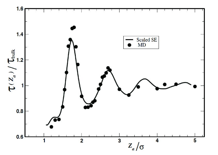
Figure 1: Average persistence time relative to the corresponding bulk value, as a function of layer position $z_{a}$. $L=0.5\sigma$. Dots are the result from the MD simulation $\left(\frac{\tau_{{}_{MD}}(z_{a})}{\tau^{bulk}_{{}_{MD}}}\right)$ clor . The continuous line is the result of scaling $\left(\frac{\tau_{{}_{{\color[rgb]{0,0,0}SE}}}(z_{a})}{\tau^{bulk}_{{}_{{\color[rgb]{0,0,0}SE}}}}\right)$ by the factor $\left[\frac{D(z_{a})}{D^{bulk}}\right]$ according to Eqs. (13) and (29).

As discussed in clor , the numerical MD value of $\tau^{bulk}_{{}_{MD}}$ gives a value of $D^{*}=1.69512\,\,\mbox{x}\,\,10^{-9}\,\,m^{2}/s$ which differs from the expected value of the bulk diffusion constant $D^{bulk}$. This is due to the known difference in the MD and SE average persistence probabilities and, by definition, of $\tau_{{}_{{\color[rgb]{0,0,0}SE}}}$ and $\tau_{{}_{MD}}$, for the same value of the virtual layer width $L$. Since this is a systematic difference, we conjecture that this relation holds also for layers located at $z_{a}$ in the vicinity of an attractive wall

$$D(z_{a})\tau_{{}_{{\color[rgb]{0,0,0}SE}}}(z_{a}) = D^{*}\tau_{{}_{MD}}(z_{a}),$$ (34)

$$= \left[\frac{L^{2}}{12}\right]\left(\frac{\tau_{{}_{MD}}(z_{a})}{\tau^{bulk}_{{}_{MD}}}\right),$$

$$= \left[D^{bulk}\,\tau^{bulk}_{{}_{{\color[rgb]{0,0,0}SE}}}\right]\left(\frac{\tau_{{}_{MD}}(z_{a})}{\tau^{bulk}_{{}_{MD}}}\right).$$

This can be rearranged as

$$\left(\frac{\tau_{{}_{MD}}(z_{a})}{\tau^{bulk}_{{}_{MD}}}\right)=\left(\frac{\tau_{{}_{{\color[rgb]{0,0,0}SE}}}(z_{a})}{\tau^{bulk}_{{}_{{\color[rgb]{0,0,0}SE}}}}\right)\left[\frac{D(z_{a})}{D^{bulk}}\right].$$ (35)

This relationship is our main result. The left hand side of this relationship corresponds to a quantity obtained directly from the persistence probability in the Molecular Dynamics simulation, using Eqs. (5) and (6). The right hand side of Eq. (35) is a quantity that can be evaluated independently from the solution of the Smoluchowski equation, Eq. (29). It contains the phenomenological diffusion coefficient, introduced in the Langevin equation, Eq. (14), in the high friction limit, Eq. (15), to relate the fluctuation and dissipation forces, $D(z)=\frac{1}{2}(\frac{\sigma(z)}{\gamma(z)})^{2}$. In Fig. 1 we plot the space average mean exit time $\tau_{{}_{{\color[rgb]{0,0,0}SE}}}(z_{a})$ as a function of the position of the virtual layer $z_{a}$. The continuous line is the result of scaling $\left(\frac{\tau_{{}_{{\color[rgb]{0,0,0}SE}}}(z_{a})}{\tau^{bulk}_{{}_{{\color[rgb]{0,0,0}SE}}}}\right)$ by the factor $\left[\frac{D(z_{a})}{D^{bulk}}\right]$ according to Eqs. (13) and (29). The quantity $[D(z_{a})\,\tau_{{}_{{\color[rgb]{0,0,0}SE}}}(z_{a})]$ was numerically evaluated from Eq. (29), using as input only the equilibrium local particle density $\rho(z)$. As we can see, from Fig. 1 the scaling of the SE and MD predicted by Eq. (35) gives a very good numerical agreement.

VI Conclusions

Once the relaxation time of the persistence probability is identified as the space average of the mean first passage time, the evaluation of the quantity $[D(z_{a})\,\tau_{{}_{{\color[rgb]{0,0,0}SE}}}(z_{a})]$ is easily obtained in terms of the equilibrium local particle density for a highly anisotropic dense fluid, next to an attractive surface. We have obtained a relationship, Eq. (35), which shows the correspondence with the VLMD value, for a fixed width of the absorbing virtual layer. The simple scaling factor in terms of the anisotropic diffusion coefficient is physically meaningful, since $D(z)$ is introduced in the Langevin equation to account phenomenologically for the fluctuation–dissipation theorem.

- (1) Colmenares, P. J.; López, F.; Olivares–Rivas, W. Phys. Rev. E 2009, 80, 061123.
- (2) Liu, P.; Harder, E.; Berne, B. J. J. Phys. Chem. B, 2004, 108, 6595.
- (3) Burschka, M. A.; Titulaer, U. M. J. Stat. Phys. 1981, 25, 569.
- (4) Harris, S. J. Chem. Phys. 1981, 75, 3103.
- (5) Razi Naqvi, K.; Mork K. J.; Waldenstrøm, S. Phys. Rev. Letts. 1982, 49, 304.
- (6) Thomas, J. A.; McGaughey, J. H. J. Chem. Phys., 2007, 126, 0347071.
- (7) Gardiner, C. W. Handbook of Stochastic Methods for Physics, Chemistry and the Natural Sciences; Springer–Verlag: Berlin, 1985.
- (8) Colmenares, P. J.; Olivares–Rivas, W. Phys. Rev. E 1999, 59, 841.
- (9) Sulbarán, B.; Olivares–Rivas, W.; Villegas, J. C.; Colmenares, P. J.; López, F. J. Mol. Struct.: THEOCHEM, 2006, 769, 151.
- (10) Sulbarán, B.; Olivares Rivas, W.; Colmenares, P. J. Cond. Matt. Phys. 2005, 8, 303.
- (11) Israelachvili J. Intermolecular Surface Forces, 2nd. Ed., Academic Press Ltd: London, 1992.
- (12) Travis, K. P.; Gubbins, K. E. J. Chem. Phys. 2000, 112, 1984.
- (13) McQuarrie D. A. Statistical Mechanics , Harper Row: New York, 1976.
- (14) H. Risken, The Fokker-Planck Equation. Methods of Solutions and Applications. Springer, 1984.
- (15) Åkesson, T; Jönsson B; Halle B; Chang D. Y. Mol. Phys. 1986, 57, 1105.
- (16) Jönsson B.; Wenneström H. in Micelar Solutions and Microemulsions edited by S. H. Chen and R. Rajagopalan; Springer–Verlag: New York, 1990.
- (17) Szabo A.; Schulten K.; Schulten Z. J. Chem. Phys. 1980, 72(8), 4350.