Improving Quantum Clocks via Semidefinite Programming

Abstract

The accuracies of modern quantum logic clocks have surpassed those of standard atomic fountain clocks. These clocks also provide a greater degree of control, because before and after clock queries, we are able to apply chosen unitary operations and measurements. Here, we take advantage of these choices and present a numerical technique designed to increase the accuracy of these clocks. We use a greedy approach, minimizing the phase variance of a noisy classical oscillator with respect to a perfect frequency standard after an interrogation step; we do not optimize over successive interrogations or the probe times. We consider arbitrary prior frequency knowledge and compare clocks with varying numbers of ions and queries interlaced with unitary control. Our technique is based on the semidefinite programming formulation of quantum query complexity, a method first developed in the context of deriving algorithmic lower bounds. The application of semidefinite programming to an inherently continuous problem like that considered here requires discretization; we derive bounds on the error introduced and show that it can be made suitably small.

I Quantum Clocks

I.1 The Clock Protocol

Most atomic clocks are designed to lock a noisy classical oscillator to the resonance of an atomic standard. Typically, this is accomplished via the following clock interrogation protocol:

1. Preparation: The atomic system is prepared in some initial state.

2. Query: The classical oscillator and the atomic system interact. This modifies the atomic state in some way that depends on both the resonant atomic frequency $\omega_{0}$ and the frequency of the classical oscillator $\omega$.

3. Measurement: The atomic system is measured and provides some information about $\omega-\omega_{0}$.

4. Correction: The classical oscillator is adjusted based on this information, ideally reducing $|\omega-\omega_{0}|$.

This protocol must be repeated indefinitely, as the noisy classical oscillator drifts over time. Furthermore, the information gained in step 3 is always incomplete. Consequently, the frequency of the classical oscillator is never known exactly and must be described by a probability distribution. Figure 1 illustrates how this distribution changes as the clock is run. In this probabilistic perspective, our goal is to maximize our knowledge of the classical oscillator. For the purpose of maintaining an accurate clock, we minimize the phase variance of the classical oscillator with respect to the atomic frequency standard by optimizing over state preparation (step 1) and the post-query measurement (step 3). We also consider interrogations consisting of multiple queries interlaced with unitary control.

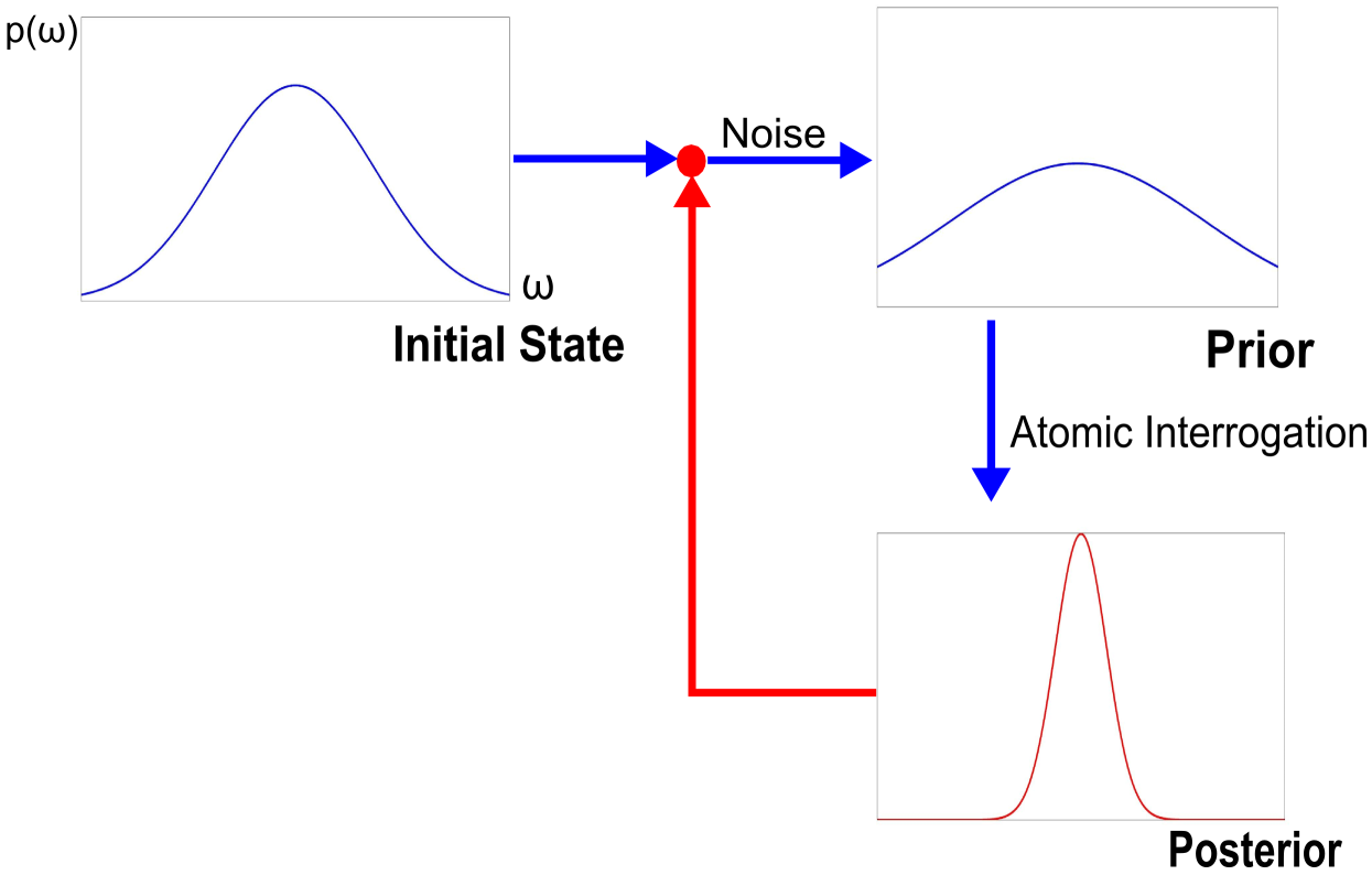
Figure 1: Evolution of the classical oscillator’s probability distribution in a clock protocol. Noise decreases our knowledge of the classical oscillator’s frequency, widening $p(\omega)$. The prior probability distribution on the right is used in our optimization procedure, and describes the average frequency of the classical oscillator over the probe time $T$. A measurement of the atomic standard then yields a measurement outcome $a$, which can be used to compute the posterior distribution $p(\omega|a)$. Over many iterations of this procedure, we gain knowledge of the history of the frequency differences. This history can be integrated to estimate the total time difference between the classical oscillator and an ideal atomic clock.

A more complete characterization of a clock involves estimating the total time difference between the clock and an ideal clock based on the atomic standard since the clock was started. The time difference is measured in terms of the total phase difference and requires integrating the frequency differences over time. A full Bayesian treatment of this characterization problem requires that we maintain the complete history of the classical oscillator by way of the joint probability distribution, $p(\omega_{1},\omega_{2}\ldots\omega_{t})$, where the marginals $p(\omega_{i})$ reflect our knowledge of the classical oscillator at a specific time in the past. However, in this paper we use a greedy approach, namely our optimization procedure does not take into account this history, and our prior knowledge consists only of the marginal $p(\omega_{t})$.

Except for a brief discussion in Sect. II.4, we ignore the effects of decoherence on the atomic standard and consider only random fluctuations of the classical oscillator’s frequency. We focus on clocks with relatively few atoms and assume full quantum control of the atoms. These clocks are often referred to as quantum clocks. An example is the highly accurate $\text{Al}^{+}$ quantum clock at NIST Schmidt et al. (2005), which is a candidate for the application of the techniques developed here.

We consider a simplified model of an $N$-atom clock, whose state is a superposition of the $N+1$ symmetric Dicke states ${|}{0}{\rangle},\ldots,{|}{N}{\rangle}$ of $N$ identical two-level systems. For example, if $N=2$, the Dicke states are given by ${|}{0}{\rangle}={|}{00}{\rangle}_{AB}$, ${|}{1}{\rangle}=({|}{01}{\rangle}_{AB}+{|}{10}{\rangle}_{AB})/\sqrt{2}$, and ${|}{2}{\rangle}={|}{11}{\rangle}_{AB}$. Ref. Bužek et al. (1999) shows that nothing can be gained by considering other states of the two-level systems. The $N$ atoms begin in the state ${|}{0}{\rangle}{\langle}{0}{|}$ and are then initialized (step 1) by the application of a unitary operator $U(0)$ to the state $\rho(0)=U(0){|}{0}{\rangle}{\langle}{0}{|}U(0)^{\dagger}$. A query (step 2) consists of the application of a second unitary operator that depends on both $\omega$ and $\omega_{0}$; normally, this dependence is only on the difference $\omega-\omega_{0}$. Then

$$\rho(0)\rightarrow\rho(0)^{\prime}=\Omega(\omega-\omega_{0})\rho(0)\Omega(\omega-\omega_{0})^{\dagger}.$$ (1)

Finally, the system is measured (step 3) with a positive operator-valued measure (POVM) $\{P_{a}\}_{a}$.

Interrogation is often done via the Ramsey technique Ramsey (1956). Here, the atoms are subject to two pulses from a classical oscillator of frequency $\omega$, separated by a period of free evolution of length $T$. These pulses are short enough for their dependence on $\omega$ to be neglected, and so for our purposes, their effect can be absorbed into the definitions of $U(0)$ and $\{P_{a}\}_{a}$. The period of free evolution is equivalent to a $z$ rotation by an angle of $(\omega-\omega_{0})T$. Thus, $\Omega(\omega-\omega_{0})$ in Eq. (1) is given by

$$\Omega(\omega-\omega_{0})=e^{-iJ_{z}(\omega_{0}-\omega)T},$$ (2)

where $J_{z}$ is the total $z$ angular momentum operator, $J_{z}{|}{k}{\rangle}=(k-N/2){|}{k}{\rangle}$. By making a global phase change, we can write the evolution of the Dicke states as

$$|k\rangle\rightarrow e^{-ik(\omega-\omega_{0})T}|k\rangle.$$ (3)

Without loss of generality, for the remainder of this paper we assume that $\omega_{0}=0$.

We refer to the action in Eq. (1) as a “clock query”. We can generalize such an action by combining multiple queries with interlaced unitary operators. The final clock state can then be written as

$$\rho(t_{f}) = \Omega(\omega)U(t_{f})\ldots\Omega(\omega)U(1)$$ (4)

$${}\times\rho(0)U^{\dagger}(1)\Omega(\omega)^{\dagger}\ldots U(t_{f})^{\dagger}\Omega(\omega)^{\dagger},$$

provided that the relative frequencies do not drift between steps 1 and $t_{f}$. We refer to the complete action in Eq. (4) as a “clock interrogation”. As written, $U(t)$ acts only on the clock’s atoms; below, we consider $U(t)$ that can also act on arbitrary ancilla atoms. Our goal is to minimize the expected cost

$$\langle C\rangle = \int\int C(\omega-f_{a})p(a|\omega)p(\omega)d\omega da$$ (5)

$$= \int\int C(\omega-f_{a})\mathrm{tr}(P_{a}\rho_{\omega}(t_{f}))p(\omega)d\omega da.$$

Here, $f_{a}$ is the classical frequency estimate for measurement outcome $a$ with associated POVM operator $P_{a}$, $p(\omega)$ is the prior probability distribution of the classical oscillator’s frequency, and $p(a|\omega)$ is the probability of measurement outcome $a$ given $\omega$ and the interrogation protocol. The subscript $\omega$ of $\rho$ indicates that the clock was interrogated by a classical oscillator at frequency $\omega$. If $C(\omega-f_{a})=(\omega-f_{a})^{2}$, then a minimization of $\langle C\rangle$ is equivalent to a minimization of the expected posterior variance of the relative phase change $\omega T$. To minimize $\langle C\rangle$ we vary the $U(t)$ in Eq. (4) and the final POVM $\{P_{a}\}_{a}$. The operator $\Omega(\omega)$ is considered fixed.

In principle one can consider simultaneously optimizing multiple sequential interrogations with varying probe times $T$. Because a fixed probe time is unable to distinguish between frequencies differing by multiples of $2\pi/T$, varying the probe time is necessary to avoid undetected frequency hops. Here, we consider only one interrogation at a time and fix the probe time $T$. In this case, there is a scaling symmetry $\omega\rightarrow\alpha\omega$ and $T\rightarrow\omega/\alpha$, so we fix $T=1$ from now on.

I.2 Background and Summary

A great deal of research has been done on the theory of atomic clock optimization. Of particular interest has been the question of how quantum effects such as entanglement and squeezing can help overcome the atomic shot-noise precision limit of $O(1/\sqrt{N})$ and approach the Heisenberg limit of $O(1/N)$ for $N$ atoms. The possibility that these effects can result in improved precision was raised in Wineland et al. (1994); Bollinger et al. (1996). These and related ideas are now at the foundations of the subject of quantum metrology Giovannetti et al. (2011). Our work is based on and extends the analytical studies of Bužek et al. Bužek et al. (1999), who sought to optimize clock interrogations under the assumption of a uniform prior and a family of periodic cost functions. Starting from results of Holevo Holevo (1982), they obtained a family of initial states that perform well for large numbers of atoms. Recently, Demkovicz-Dobrazanski Demkowicz-Dobrzanski (2011) optimized interrogations with costs determined by the periodic function $C(\omega-f_{a})=4\sin^{2}\frac{(\omega-f_{a})}{2}$ for arbitrary continuous priors. While this approach is largely analytical, its implementation requires the numerical maximization of a trace norm. These works focus on optimizing a single interrogation. Long-term stability has been analyzed for entangled states of a number of atoms in Ref. Wineland et al. (1998), and for a family of squeezing protocols of atomic ensembles in Ref. André et al. (2004). These studies account for phase noise in the classical oscillator and optimize clock protocols given specific feedback mechanisms and noise models.

The periodic cost functions studied in Bužek et al. (1999); Demkowicz-Dobrzanski (2011) are convenient for analytic studies of clock optimization but do not penalize phase errors greater than $2\pi$, even though they correspond to frequency estimates far from the true frequency of the oscillator. This issue becomes important when multiple interrogations and long-term clock stability are considered. Given that we do not explicitly consider either, and that in the model described above, phases differing by multiples of $2\pi$ cannot be distinguished, this may seem irrelevant. Specifically, when optimizing interrogations consisting of one query or multiple queries with identical probe times as we do here, the prior and the cost function can in principle be folded into the interval $[-\pi,\pi]$. However, this folding results in a cost function that depends on the prior. Because of this and in view of future extensions of this work, we consider non periodic cost functions, particularly the quadratic one.

The goal here is to apply the semidefinite programming strategy originally developed for quantum query algorithms Barnum et al. (2003); Barnum (2007) to the problem of optimizing clock interrogations. This enables the greatest flexibility in searching for solutions, as both the prior and the cost function can be arbitrary. The first major obstacle is that the unknown parameter of the queries is continuous rather than discrete and finite as in typical quantum query algorithms. We overcome this by showing how to systematically discretize the parameter spaces while having good control of the discretization errors. The second major obstacle is that the size of the semidefinite program (SDP) grows at a rate of $\Theta\left(t_{f}|O|^{2}(|Q|+|F|)\right)$, where $|O|$ is the number of points in our discretization, $|Q|$ is the number of atoms we are simulating, and $|F|$ is the number of POVM elements. This limits the number of atoms and the level of discretization for which general clock interrogations can be optimized, depending on available computational resources. We show that for small but useful numbers of atoms, the SDPs can be implemented and solved given current resources.

The semidefinite programming strategy is formulated in full generality in Sec. II. Our version does not restrict the set of possible queries or the prior over query parameters. We show how to explicitly reconstruct the algorithm and measurements from the solution and discuss how to modify the strategy to account for query noise. This may be of independent interest for interpolating between quantum and classical query complexity. In Secs. III and IV, we specialize the SDPs to the case of quantum clocks. Here we show how to discretize the parameter spaces to obtain finite SDPs while bounding discretization errors. In Sec. V we show the results from applying the discretized SDPs to concrete clock problems. In particular we compare the computational results obtained to prior work, demonstrating both the ability to obtain improvements and to determine bounds on optimal costs.

II The Semidefinite Programming Formulation of Quantum Query Complexity

II.1 Constructing the Semidefinite Program

The operation of a quantum clock can be expressed naturally in the query model of quantum computation. Here, we are given an oracle (or black box) chosen from some finite set $\{\Omega(1),\Omega(2)...\Omega(M)\}$. Each oracle $\Omega(x)$ is a unitary operator, selected with probability $p(x)$. The goal is to determine $x$ with queries, that is, with applications of $\Omega(x)$ to quantum states and measurement. Often in this context, one is interested in minimizing the number of queries needed to learn $x$ with near certainty. Here, however, we fix the number of queries and seek to minimize the expected difference between an estimate $x^{\prime}$ of $x$ and $x$ as quantified by a cost function $C(x,x^{\prime})$.

We adapt the semidefinite programming formulation of quantum query complexity developed by Barnum et  al. Barnum et al. (2003); Barnum (2007) in the context of proving quantum lower bounds. They cast the problem of determining the number of queries required in terms of a test of feasibility of a semidefinite program. Here we aim to minimize an expected cost, which requires optimizing an objective function with an extended SDP. For a general introduction to semidefinite programming see Ref. Vandenberghe and Boyd (1996).

To formulate the SDP, we introduce quantum systems $O$ and $Q$ for the oracle and the querier, respectively. System $Q$ is the one on which the oracle operators $\Omega(x)$ act. An additional system of ancillas $A$ may be used by the querier; for the purposes of the SDP, we normally trace out $A$. We use the convention that the systems on which an operator acts are denoted by superscripts. For states (density operators) $\rho$, partially omitted system superscripts imply the partial trace over the omitted systems. Superscripts may be completely omitted if the set of systems being acted on is clear or irrelevant. The dimension of the state space of system $S$ is denoted by $|S|$. Initially, the state of the oracle system is given by $\rho_{0}=\sum_{x}\sum_{y}\sqrt{p(x)}\sqrt{p(y)}{|}{x}{\rangle}{\langle}{y}{|}$. By representing the oracle probabilities with a pure superposition, we encode the fact that there is no information about $x$ available to the querier (or any system other than $O$). We define the joint operator $\Omega^{OQ}=\sum_{x}{|}{x}{\rangle}{\langle}{x}{|}\Omega^{Q}(x)$, which applies $\Omega(x)$ to system $Q$ conditional on the state ${|}{x}{\rangle}$ of the oracle. In this setting, a multi-query quantum computation is given by the composition

$$\rho^{OQA}(t_{f})=\Omega^{OQ}U^{QA}(t_{f})\ldots\Omega^{OQ}U^{QA}(1)\rho^{OQA}(0)U^{\dagger QA}(1)\Omega^{\dagger OQ}\ldots U^{\dagger QA}(t_{f})\Omega^{\dagger OQ}$$ (6)

followed by a measurement of $QA$ with a POVM. Here $\rho^{OQA}(0)$ is the initial state, with $\rho^{O}(0)=\rho_{0}$ pure as defined above, and $\rho^{QA}(0)$ is a state chosen by the querier. The unitary operators $U^{QA}(t)$ are inter-query operators that can be chosen arbitrarily for each step $t$. The querier’s protocol (or algorithm) is determined by the initial state $\rho^{QA}(0)$, the $U^{QA}(t)$, and the POVM. Refs. Barnum et al. (2003); Barnum (2007) show that there is a correspondence between these algorithms and solutions to a set of semidefinite constraints. We split the constraints into those that correspond to the initial state and choice of inter-query operators, and those that correspond to the POVM. The first set, $S_{E}$, consists of

1. $\rho^{O}(0)=\rho_{0}$,

2. and the following for $t\in\{0,1,\ldots,t_{f}\}$:

3. $\rho^{OQ}(t)\geq 0$,

4. $\rho^{O}(t)=tr_{Q}(\rho^{OQ}(t))$ and

5. $\rho^{O}(t)=tr_{Q}(\Omega^{\dagger OQ}\rho^{OQ}(t-1)\Omega^{OQ})$.

The constraints corresponding to the POVM and the objective to be optimized can be based on a connection to the concept of remote state preparation as described next.

II.2 Measurement and Remote State Preparation

Remote state preparation Hughston et al. (1993) involves two systems $O$ and $Q$. Given a joint state of the two systems, we can prepare states of $O$ conditional on measurements of $Q$.

Definition 1.

We say that we can remotely prepare $\{\sigma_{a}^{O}\}_{a}$ from the state $\rho^{OQ}$ on $O$ and $Q$ if there exists a POVM of $Q$ with operators $\{P_{a}^{Q}\}_{a}$ such that $tr_{Q}(P_{a}^{Q}\rho^{QO})=\sigma_{a}^{O}$.

The members $\sigma_{a}^{O}$ of the set that can be remotely prepared are positive operators with trace $0\leq\mathrm{tr}(\sigma_{a}^{O})\leq 1$. The definition implies that the state $\sigma_{a}^{O}/\mathrm{tr}(\sigma_{a}^{O})$ can be conditionally prepared with probability $\mathrm{tr}(\sigma_{a}^{O})$ by means of a fixed POVM on $Q$. For definiteness, consider a POVM $\{P_{a}^{Q}\}$. Any implementation of the POVM has the desired effect. Such an implementation is described by a quantum operation with Kraus operators $E_{a}$ such that $E_{a}^{\dagger}E_{a}=P_{a}$. For outcome $a$, the unnormalized $OQ$ state is $E_{a}^{Q}\rho^{OQ}E_{a}^{\dagger Q}$. Cyclicity of partial trace implies that $\mathrm{tr}_{Q}E_{a}^{Q}\rho^{OQ}E_{a}^{\dagger Q}=\mathrm{tr}_{Q}P_{a}^{Q}\rho^{OQ}=\sigma_{a}^{O}$. The probability of the outcome is $\mathrm{tr}(\sigma_{a}^{O})$.

Theorem 1 characterizes the set of states that can be remotely prepared according to Def. 1 from a pure state.

Theorem 1.

Let $\rho^{OQ}$ be a pure state of systems $O$ and $Q$. We can remotely prepare $\{\sigma_{a}^{O}\}_{a}$ if and only if $\sum_{a}\sigma^{O}_{a}=\rho^{O}$.

The proof of Thm. 1 is given in App. A.

In order to apply Thm. 1 we formulate the expected cost in terms of the POVM-conditional unnormalized states $\sigma_{a}^{O}$. In the clock problem, the querier associates an estimated frequency $f_{a}$ with each measurement outcome $a$. Assume for simplicity that the possible classical oscillator frequencies $\omega$ come from a finite set. We can define operators $A_{a}^{O}$ in the oracle basis $\{{|}{\omega}{\rangle}\}_{\omega}$ by $(A_{a})_{\omega,\omega^{\prime}}=\delta_{\omega,\omega^{\prime}}C(\omega-f_{a})$. Eq. (5) can be rewritten as

$$\langle C\rangle=\sum_{a}\mathrm{tr}(A_{a}\sigma_{a}).$$ (7)

With this equation as motivation, we consider the general situation where the expected cost of a querier protocol is computed from predetermined cost operators $A_{a}$ according to the POVM-conditional oracle states as in Eq. (7). This motivates the following SDP $S_{M}(\rho^{O})$ for a given oracle state $\rho^{O}$:

$$\text{Minimize $\mathrm{tr}(\sum_{a}\sigma_{a}A_{a})$ subject to:}\begin{cases}\forall a\sigma_{a}\geq 0,\\ \sum_{a}\sigma_{a}=\rho^{O}.\end{cases}$$ (8)

Theorem 2.

Suppose that $\rho^{OQA}$ is pure. Then $S_{M}(\rho^{O})$ computes the minimum expected cost over measurements on $QA$.

Proof.

It suffices to observe that according to Thm 1, sets $\{\sigma_{a}\}_{a}$ satisfying the constraints of $S_{M}$ are precisely the sets that can be remotely prepared with access to systems $QA$. ∎

The complete SDP for the query optimization problem is obtained by combining $S_{Q}=S_{E}\cup S_{M}(\rho^{O}(t_{f}))$. Because query algorithms have access to the non-$O$ systems of a purification of $\rho^{O}(t_{f})$, $S_{Q}$ computes the optimal average cost of a $t_{f}$-query quantum algorithm. The SDP considered in the spectral adversary method Barnum et al. (2003); Barnum (2007) is a relaxation of $S_{Q}$ with a modified objective designed to determine a lower bound on the number of queries needed to obtain some fixed probability of error. There has been significant recent progress in refining this relaxation Hoyer et al. (2007) and demonstrating that it is nearly exact Lee et al. (2010). Note that in our case, we can construct cost operators $A_{a}$ such that $S_{Q}$ minimizes the probability of error for fixed $t_{f}$.

II.3 Algorithm and POVM reconstruction

For any solution of $S_{Q}$, in particular the optimal one, there is an explicit query algorithm that achieves the associated cost objective. In particular, given the sequence of density matrices $\rho^{OQ}(t)$ and the conditional operators $\sigma_{a}$, it must be possible to infer the sequence of unitaries in Eq. (6) and the POVM achieving the expected cost. The POVM yielding the conditional operators $\sigma_{a}$ can be constructed as in the proof of Thm. 1. To determine the unitaries $U^{QA}(t)$, first extend the querier system with an ancilla $A$, where $A$ has dimension $|O||Q|$. For each $t$, construct pure states $\rho^{\prime OQA}(t)$ and $\rho^{OQA}(t+1)$ by purifying $\rho^{\prime OQ}(t)=\Omega^{\dagger OQ}\rho^{OQ}(t)\Omega^{OQ}$ and $\rho^{OQ}(t+1)$, respectively. By construction, $\rho^{\prime O}(t)=\rho^{O}(t+1)$. One can therefore use the Schmidt forms for the pure states $\rho^{\prime OQA}(t)$ and $\rho^{OQA}(t+1)$ to construct unitaries $U^{QA}(t)$ satisfying

$$\rho^{OQA}(t+1)=U^{QA}(t)\rho^{{}^{\prime}OQA}(t)U^{\dagger QA}(t).$$ (9)

II.4 Noise

The SDP $S_{Q}$ is based on the assumption that there is no noise in the query process. In particular, this excludes decoherence during clock queries. It is possible to adapt $S_{Q}$ to include the effects of noise. This requires that we extend the states $\rho^{OQ}$ by querier-inaccessible systems $E_{i}$ modeling the environments causing the noise. The net effect of query and noise can be modeled by an oracle-conditional isometry defined by

$${|}{x}{\rangle}{\langle}{y}{|}\rho^{Q}\rightarrow{|}{x}{\rangle}{\langle}{y}{|}\Omega(x)^{QE}\rho^{Q}{|}{\epsilon}{\rangle}{\langle}{\epsilon}{|}\Omega(y)^{\dagger QE},$$ (10)

where ${|}{x}{\rangle},{|}{y}{\rangle}$ are the standard oracle basis states, ${|}{\epsilon}{\rangle}$ is a fixed initial state of $E$ and $\Omega(x)^{QE}$ is unitary. Define $\Omega^{OQE}=\sum_{x}{|}{x}{\rangle}{\langle}{x}{|}\Omega(x)^{QE}$. In the absence of noise, $\Omega(x)^{QE}={\langle}{x}{|}\Omega^{OQ}{|}{x}{\rangle}$. In many cases one can decompose $\Omega(x)^{QE}=D^{QE}{\langle}{x}{|}\Omega^{OQ}\otimes I^{E}{|}{x}{\rangle}$ for an $O$-independent unitary $D^{QE}$. An example is the clock query in the presence of phase decoherence. In a sequence of queries, a new version of $E$, $E_{i}$ is introduced at each step by the isometry. Let $E^{t}=E_{1}E_{2}\ldots E_{t}$. To account for the noisy query, the SDP $S_{Q}$ is modified to $S_{D}$ as follows:

Min $$\text{imize\ }\mathrm{tr}(\sum_{a}\sigma_{a}^{OE^{t_{f}}}A_{a}^{O})\text{\ subject to}$$

$$\sigma_{a}^{OE^{t_{f}}}\geq 0$$

$$\sum_{b}\sigma_{b}^{OE^{t_{f}}}=\rho^{OE^{t_{f}}}(t_{f})$$

$$\rho^{OE^{t}Q}(t)\geq 0$$

$$\rho^{OE{{}^{t}}}(t)=tr_{Q}(\rho^{OE^{t}Q}(t))$$

$$\rho^{OE^{t}}(t)=tr_{Q}\left(\Omega^{OQE_{t}}\rho^{OE^{t-1}Q}(t-1){|}{\epsilon}{\rangle}{\langle}{\epsilon}{|}\Omega^{\dagger OQE_{t}}\right)$$

$$\rho^{OE^{0}}(0)=\rho_{0}.$$

(There is an implicit “for all” over the free variables $a$ and $t$.)

Phase decoherence is a particularly interesting example of this more general SDP. As mentioned above, for complete phase decoherence, the query isometry factors, in this case giving

$$D^{QE}{|}{i}{\rangle}^{Q}{|}{\epsilon}{\rangle}^{E}={|}{i}{\rangle}^{Q}{|}{\epsilon_{i}}{\rangle}^{E},$$ (11)

where the ${|}{\epsilon_{i}}{\rangle}$ are orthonormal states. The effect is to perfectly correlate the environment at each step with the standard query basis. In the context of standard query algorithms with a cost function that captures the probability of successfully identifying the oracle, the optimal solution to the SDP with complete phase decoherence corresponds to an optimal classical query algorithm for the given number of queries $t_{f}$. By modifying $D^{QE}$ to model incomplete phase decoherence, it is possible to interpolate between classical and quantum query algorithms, albeit at the large cost of adding the systems $E_{i}$.

Note that it is not possible to simply trace out the $E_{i}$ in the SDP: As can be seen from the method of reconstructing the algorithm from a solution of the SDP, this would be equivalent to giving the querier access to the $E_{i}$. That is, the querier has implicit access to anything that gets traced out, since traced out systems are not constrained by the SDP. When the noisy query factors, this is equivalent to not having had any noise at all, because the querier can just undo the noise isometries.

III The Clock SDP

One can apply the SDP $S_{Q}$ to the clock problem, but the result is not finitely implementable because the oracle system $O$ is continuous and the cost operators are continuously indexed. To make the SDP finite, we discretize both the possible oracle frequencies and the frequency estimates that determine the cost operators. In particular, we constrain $\omega\in\{\omega_{1},\ldots,\omega_{d}\}$, and restrict the measurement outcomes to a finite set $a\in\{1,\ldots,m\}$ associated with the set of frequency estimates $F=\{f_{a}\}_{a=1,\ldots,m}$. The frequency estimates need not be among the $\omega_{i}$. The query system $Q$’s Hilbert space is spanned by the Dicke states ${|}{k}{\rangle}$. The oracle initial state is given by

$$\rho^{O}(0)=\sum_{x,y}\sqrt{p(\omega_{x})p(\omega_{y})}{|}{x}{\rangle}{\langle}{y}{|},$$ (12)

where $p(\omega_{x})$ is the prior probability of $\omega_{x}$, a discretization of the continuous prior, and ${|}{x}{\rangle}$ is the oracle basis state corresponding to classical oscillator frequency $\omega_{x}$. The operator $\Omega^{OQ}$ is now given by

$$\Omega^{OQ}=\sum_{x}{|}{x}{\rangle}{\langle}{x}{|}\exp(-iJ_{z}^{Q}\omega_{x}),$$ (13)

up to irrelevant $x$-dependent phases. As noted before Eq. (7), the cost operators are given by

$$(A_{a})_{x,y}=C(\omega_{x}-f_{a})\delta(x,y).$$ (14)

Since the SDP depends on $p$ and $F$, we denote it by $S_{C}(p,F)$. We also use $S_{C}(p,F)$ to denote the optimum achievable cost given $p$ and $F$. For discretized prior and frequency estimates, this is the cost computed by the SDP.

As written, the size of the SDP $S_{Q}$ is $\Theta\left(t_{f}|O|^{2}(|Q|^{2}+|F|)\right)$, where $F=\{f_{a}\}$. Our implementation of the SDP takes advantage of the fact that for the clock problem, $\Omega$ is diagonal in the Dicke basis, thus reducing the size and therefore the memory and time resources required to solve the SDP. In particular, the set of solutions is invariant under the transformation $\rho^{OQ}(t)\rightarrow U(t)^{Q}\rho^{OQ}(t)U(t)^{\dagger Q}$ for operators $U(t)$ diagonal in the Dicke basis. It follows that we can restrict the SDP by assuming $\rho^{Q}(t)$ is diagonal. The restricted SDP’s size is $\Theta\left(t_{f}|O|^{2}(|Q|+|F|)\right)$.

IV Discretization Error

When solving the SDP, it is necessary to make an estimate of the difference between the discretized SDP’s optimal cost and that of the infimum of the costs of solutions to the continuous problem. We separately bound the error due to discretizing the prior (oracle discretization) and that due to discretizing the measurement outcomes (querier discretization). To deal with the oracle discretization error, we solve clock SDPs with random oracle discretizations so that the average cost for different discretizations is a lower bound on the optimum cost of the continuous problem. An upper bound is obtained by a cost integral applied to any of the SDPs solved. For the quadratic cost function, the querier discretization error can be bounded in a way that depends only on the set $F=\{f_{a}\}_{a}$ and can be made to go to zero by increasing the size and resolution of $F$. We start with querier discretization.

IV.1 Querier Discretization Error

To guarantee that we determine the optimum cost for a frequency prior $p$, the set of allowed querier frequency estimates $F$ should be all of $\mathbb{R}$. To solve the clock SDP numerically, we restrict $F$ to a finite subset. By definition, $S_{C}(p,F)\geq S_{C}(p,\mathbb{R})$. The goal of this section is to obtain a lower bound on $S_{C}(p,\mathbb{R})$ depending on $F$, and to explain an iterative strategy for locally optimizing $F$. Let $F=\{f_{1},\ldots,f_{N}\}$ with $f_{j}<f_{j+1}$.

Theorem 3.

Let $C$ be a second differentiable, non-negative function satisfying $C^{\prime\prime}(x)\leq b$, $C(0)=0$ and $C$ is monotone on $[0,\infty)$ and $(-\infty,0]$. Define $M(\omega)$ by

$$M(\omega)=\begin{cases}C(\omega-f_{1})&\text{for\ }\omega\leq f_{1}\\ C(\omega-f_{N})&\text{for\ }\omega\geq f_{N}\\ 0&\text{otherwise}\end{cases}$$ (15)

We have the following inequality:

$$S_{C}(p,F)-S_{C}(p,\mathbb{R}) \leq \max_{j}\frac{b}{8}(f_{j+1}-f_{j})^{2}$$ (16)

$${}+\int M(\omega)p(\omega)d\omega.$$

The proof is in App. B. A strategy for obtaining an initial choice of an $N$-point $F$ is to optimize the right-hand-side of Eq. (16).

An important question is how many frequency estimates $f_{a}$ are needed so that $S_{C}(p,F)=S_{C}(p,\mathbb{R})$. One can obtain an upper bound by observing that the rank $r$ of the final oracle density matrix $\rho^{O}(t_{f})$ is bounded by $|Q|^{t_{f}}$ and $|O|$, where $|Q|$ and $|O|$ are the dimensions of the query and oracle systems. From this one finds that the optimal POVM can always be reduced to at most $r^{2}$ elements, implying that a set $F$ with $|F|\leq r^{2}$ suffices. There is evidence that a smaller set is optimal for the clock problem. For $t_{f}=1$ and for some costs and priors, we need only $|F|=r$ elements. Derka et al. (1998); Demkowicz-Dobrzanski (2011).

At present, we have no provably correct way of choosing the finite set of frequency estimates optimally. However, for the quadratic cost function $C(x)=x^{2}$, the following heuristic is often effective at optimizing the choices given an oracle discretization. We begin with any set of estimates. We then run the SDP and use the solution to compute the posterior distribution for each measurement outcome:

$$p(\omega|f_{a})=\frac{p(f_{a},\omega)}{p(f_{a})}=\frac{(\sigma_{a})_{\omega,\omega}}{\mathrm{tr}(\sigma_{a})},$$ (17)

where the $\sigma_{a}$ are the measurement-conditional unnormalized oracle states at the end of the algorithm. Next, we compute the mean of each of these distributions:

$$\langle\omega|a\rangle=\sum_{x}\frac{(\sigma_{r})_{x,x}}{\mathrm{tr}(\sigma_{a})}\,\omega_{x},$$ (18)

where $x$ indexes the finite set of frequencies and the expression in angle brackets is the average of $\omega$ given that measurement outcome $a$ was obtained. Replacing the original estimates $f_{a}$ by their posterior means is guaranteed to improve the cost without having to change the algorithm. We then run the SDP again, replacing the frequency estimate $f_{a}$ with $\langle\omega|a\rangle$. This procedure is repeated until each estimate is numerically close to its posterior mean. The procedure can be adapted to other costs, but the mean must be replaced by a statistic appropriate for the cost. For example, for $C(x)=|x|$ we compute the median instead of the mean.

IV.2 Oracle Discretization Error

Let $p(\omega)$ be the probability density of the prior distribution of clock frequencies. For simplicity, we assume that the prior distribution is absolutely continuous with respect to Lebesgue measure. Let $P(\omega)$ be the cumulative distribution function of $p(\omega)$, and $P^{-1}$ its inverse on $(0,1)$. Given an offset $o\in(0,1/d)$, we can define the probability distribution

$$p_{o}(\omega)=\sum_{k=0}^{d-1}\frac{1}{d}\delta_{P^{-1}(o+k/d)}(\omega).$$ (19)

This is an instance of a discretized prior. Define $\omega(k,o)=P^{-1}(o+k/d)$. The distribution $p_{o}$ is designed to approximate $p$ as $d$ goes to infinity. If we choose $o$ uniformly at random from $(0,1/d)$, it is identical to $p$. Specifically,

$$\int_{o=0}^{1/d}p_{o}(\omega)p(o)do$$

$$=\int_{o=0}^{1/d}d\sum_{k=0}^{d-1}\frac{1}{d}\delta_{\omega(k,o)}(\omega)do=p(\omega).$$ (20)

This follows from inverse transform sampling Devroye (1986) (pg. 28).

To estimate the optimum cost $S_{C}(p,F)$, we estimate the average $\langle S_{C}(p_{o},F)\rangle_{o\in(0,1/d)}$ by solving $S_{C}(p_{o},F)$ for a number of offsets $o$ chosen uniformly at random from $(0,1/d)$. According to the next theorem, this gives a lower bound on $S_{C}(p,F)$. We assume that the frequency estimates have already been discretized, $F=\{f_{a}\}_{a}$.

Theorem 4.

The following inequality holds: $\langle S_{C}(p_{o},F)\rangle_{o}\leq S_{C}(p,F)$.

Proof.

Consider an arbitrary query algorithm ${\cal Q}$. Given a prior $r(\omega)$, ${\cal Q}$ results in the measurement-conditional, unnormalized oracle states $\sigma_{a}(r,{\cal Q})$. Because the cost operators are diagonal, we can consider just the diagonals of the $\sigma_{a}(r,{\cal Q})$, which define the joint probability distributions $r(a,\omega|{\cal Q})$. Because the oracle operators are conditional on the standard oracle basis, $r(a,\omega|{\cal Q})$ factors as

$$r(a,\omega|{\cal Q})=q(a|\omega,{\cal Q})r(\omega),$$ (21)

where, as indicated, the distribution $q$ does not depend on $r$.

The average cost for ${\cal Q}$ and $r$ is given by

$$C(r,{\cal Q})=\sum_{a}\int C(\omega-f_{a})r(a,\omega|{\cal Q})d\omega.$$ (22)

If ${\cal Q}_{\min}$ is an optimal algorithm for $S_{C}(r,F)$, then for any algorithm ${\cal Q}$, it follows that $C(r,{\cal Q})\geq C(r,{\cal Q}_{\min})=S_{C}(r,F)$. Let ${\cal Q}_{o}$ and ${\cal Q}_{\text{opt}}$ be optimal algorithms for $S_{C}(p_{o},F)$ and $S_{C}(p,F)$, respectively. Then

$$\langle S_{C}(p_{o},F)\rangle_{o} =\langle C(p_{o},{\cal Q}_{o})\rangle_{o}$$

$$\leq\langle C(p_{o},{\cal Q}_{\text{opt}})\rangle_{o},$$ (23)

where the subscript on the expectations indicates that they are taken with respect to the distribution over offsets $o$. The intuition here is that we can obtain a lower cost if we are able to choose a different algorithm ${\cal Q}_{o}$ for different choices of $o$, than if we are forced to use the same algorithm ${\cal Q}_{\text{opt}}$ in all cases. We can continue from the last line of Eq. (23) as follows:

$$\langle C(p_{o},{\cal Q}_{\text{opt}})\rangle_{o}$$

$$=\left\langle\sum_{a}\int C(\omega-f_{a})p_{o}(a,\omega|{\cal Q}_{\text{opt}})d\omega\right\rangle_{o}$$

$$=\left\langle\sum_{a}\int C(\omega-f_{a})q(a|\omega,{\cal Q}_{\text{opt}})p_{o}(\omega)d\omega\right\rangle_{o}$$

$$=\sum_{a}\int C(\omega-f_{a})q(a|\omega,{\cal Q}_{\text{opt}})\langle p_{o}(\omega)\rangle_{o}\,d\omega.$$ (24)

Combining Eqs. (IV.2),(23),(24) then gives

$$\langle S_{C}(p_{o},F)\rangle_{o} \leq\sum_{a}\int C(\omega-f_{a})q(a|\omega,{\cal Q}_{\text{opt}})p(\omega)d\omega$$

$$=C(p,{\cal Q}_{\text{opt}})=S_{C}(p,F),$$ (25)

proving the claim of the theorem. ∎

We note that Thm. 4 generalizes to arbitrary oracle problems where the cost operators $A_{a}$ are diagonal. Furthermore, the proof works for any family of probability distributions $p_{o}$ such that $p$ is a mixture of the $p_{o}$.

Upper bounds on the optimal expected costs can be obtained by applying the inequality in the next Theorem.

Theorem 5.

Let ${\cal Q}$ be an algorithm for $S_{C}(r,F)$. Then

$$S_{C}(p,F)\leq\sum_{a}\int C(\omega-f_{a})q(a|\omega,Q)p(\omega)d\omega.$$ (26)

Proof.

The right-hand-side is the expected cost for algorithm ${\cal Q}$ given oracle prior $p$. Since ${\cal Q}$ is optimal for prior $r$ but not necessarily for $p$, this must be greater than $S_{C}(p,F)$, which is the optimum expected cost for prior $p$. ∎

In view of the results of this section, we adopt the following procedure ${\cal A}(p,F)$ for estimating a lower bound and calculating an upper bound of $S_{C}(p,F)$.

1. Choose discretization parameter $d$ and the number of random samples $k$. Large $d$ should tighten the bounds. Large $k$ improves the statistical estimate of the lower bound.

2. Independently choose $o_{j}\in(0,1/d)$, $j\in\{1,\ldots,k\}$ uniformly at random.

3. Do the following for each $j\in\{1,\ldots,k\}$:

   1. Compute the optimum cost $C_{j}=S_{C}(p_{o_{j}},F)$, and from the SDP solution, reconstruct an optimal algorithm ${\cal Q}_{j}$ achieving this cost.

   2. From ${\cal Q}_{j}$ derive an algorithm for evaluating $q(a|\omega,{\cal Q}_{j})$.

   3. Using this algorithm, evaluate

      $$\overline{C_{j}}=\sum_{a}\int C(\omega-f_{a})q(a|\omega,{\cal Q})p(\omega)d\omega$$

      by numerical integration.

4. Return $\frac{1}{k}\sum_{j}C_{j}$ as a statistical estimate of a lower bound (together with its estimated error) and $\min_{j}(\overline{C_{j}})$ as a numerical upper bound.

IV.3 Procedure for Solving the Clock SDP

Combining the ideas of this section, we use the following procedure for approximately solving the clock SDP $S_{C}(p,\mathbb{R})$:

1. Choose a discretization $F$, $|F|=m$, of the frequency estimates. If the cost function is suitable, we can optimize the right-hand-side of Eq. 16 and let $\epsilon_{q}$ be the corresponding querier discretization error bound.

2. Apply procedure ${\cal A}(p,F)$ and let $c_{l}$ be the statistically estimated lower bound with estimated standard error $s_{l}$, and $c_{u}$ the numerical upper bound obtained.

3. Give the estimated cost of $S_{C}(p,\mathbb{R})$ in the form $((c_{l}-\epsilon_{q})\pm s_{l},c_{u})$.

If the cost function is not suitable, we set $\epsilon_{q}=0$ and describe the discretization $F$ for which the bounds apply.

V Results

We begin by considering one-query clock protocols ($t_{f}=1$). In this case the protocol consists of an initial query state to be prepared and a final measurement. Figures 2 and 3 illustrate the importance of taking into account prior knowledge when deriving optimal clock protocols. Here our technique is compared to that of Ref. Bužek et al. (1999), which derives protocols under the assumption that $\omega$ is uniformly distributed on $[-\pi,\pi]$. We consider Gaussian priors of various widths and see that solving the clock SDP can substantially reduce the expected cost. If we use the periodic cost function $4\sin^{2}(\frac{\omega-\omega_{a}}{2})$ considered in Bužek et al. (1999), in the limit of wide prior, we obtain identical protocols. This is illustrated by Table 1, which lists initial $2$-atom states that optimize this cost function; the final row corresponds to the state computed in Ref. Bužek et al. (1999).

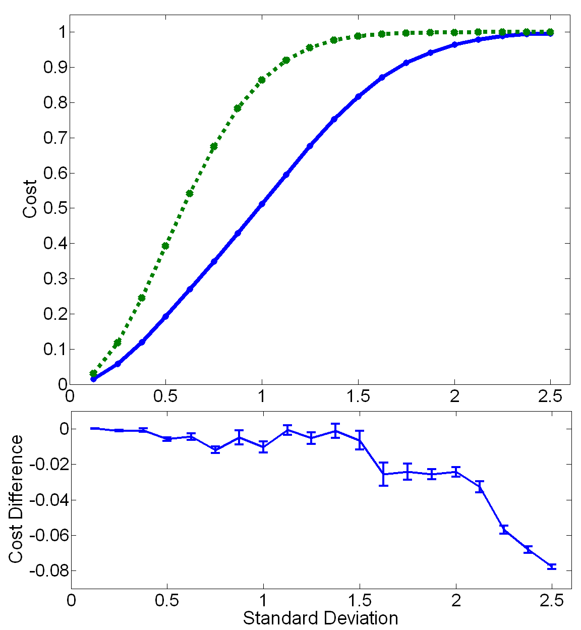
(a)  One atom

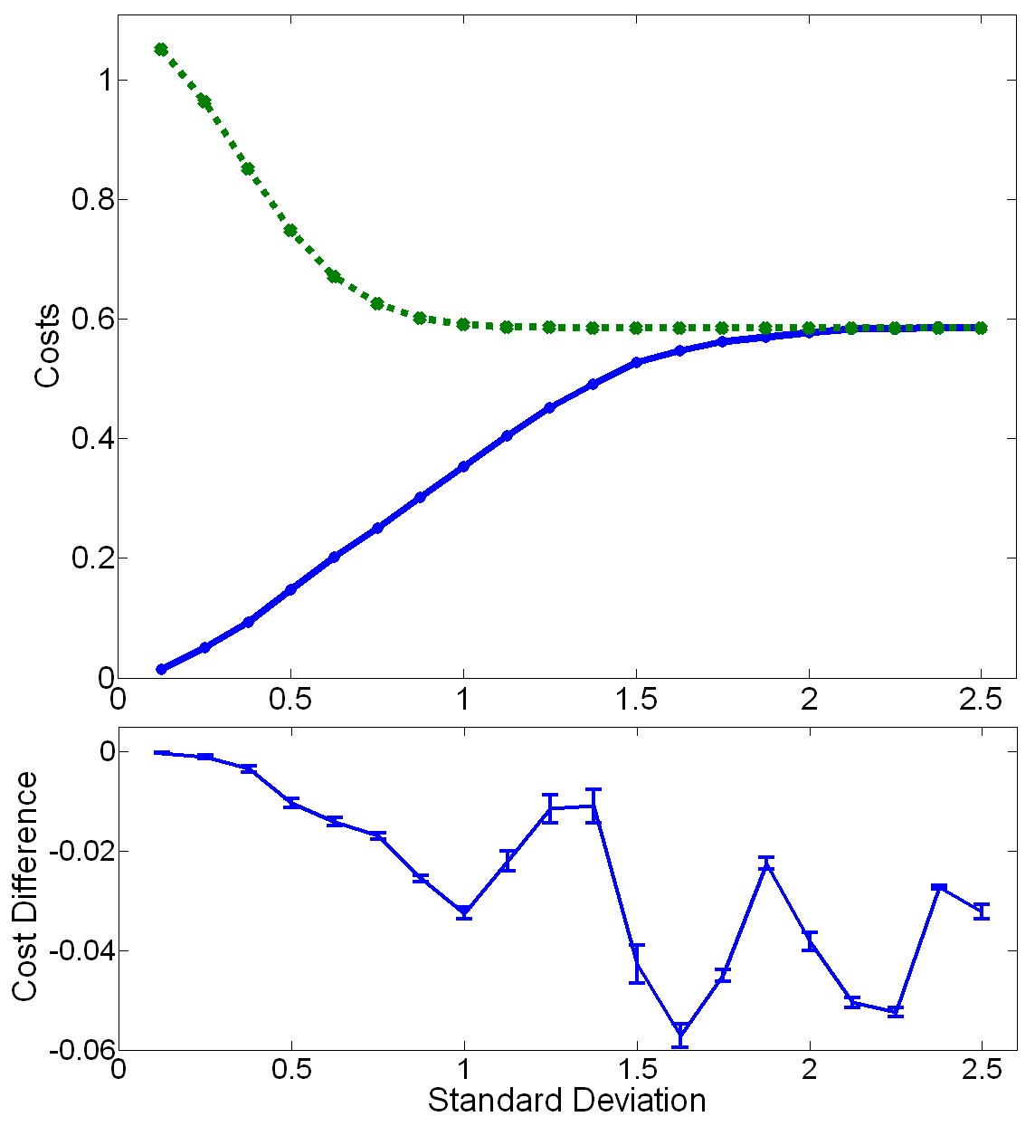
(b)  Two atoms

Figure 2: Comparison of the protocol derived in Ref. Bužek et al. (1999) and those derived by our method for one and two atoms and the cost function $C(\omega-f_{a})=4\sin^{2}(\frac{\omega-f_{a}}{2})$. We use a $15$-point oracle discretization, $20$ frequency estimates, and simulate Gaussian priors of various widths. The figures on the top plot the cost computed in Ref. Bužek et al. (1999) (dashed line) and our numerical upper bound (solid line), which as discussed, is equivalent to the minimum continuous cost obtained by one of our extracted algorithms. The figures on the bottom plot the difference between our lower bound and upper bound, $c_{l}-c_{u}$, illustrating both the strength of our bounds and how much lower the continuous cost could potentially be. The lower bound was computed by averaging $100$ discretizations; error bars show the estimated standard error of the average thus obtained. Our querier discretization bounds cannot be applied to the periodic cost function used here, so the lower bounds are for the discretizations chosen. The lines connecting the data points in our figures are to guide the eyes.

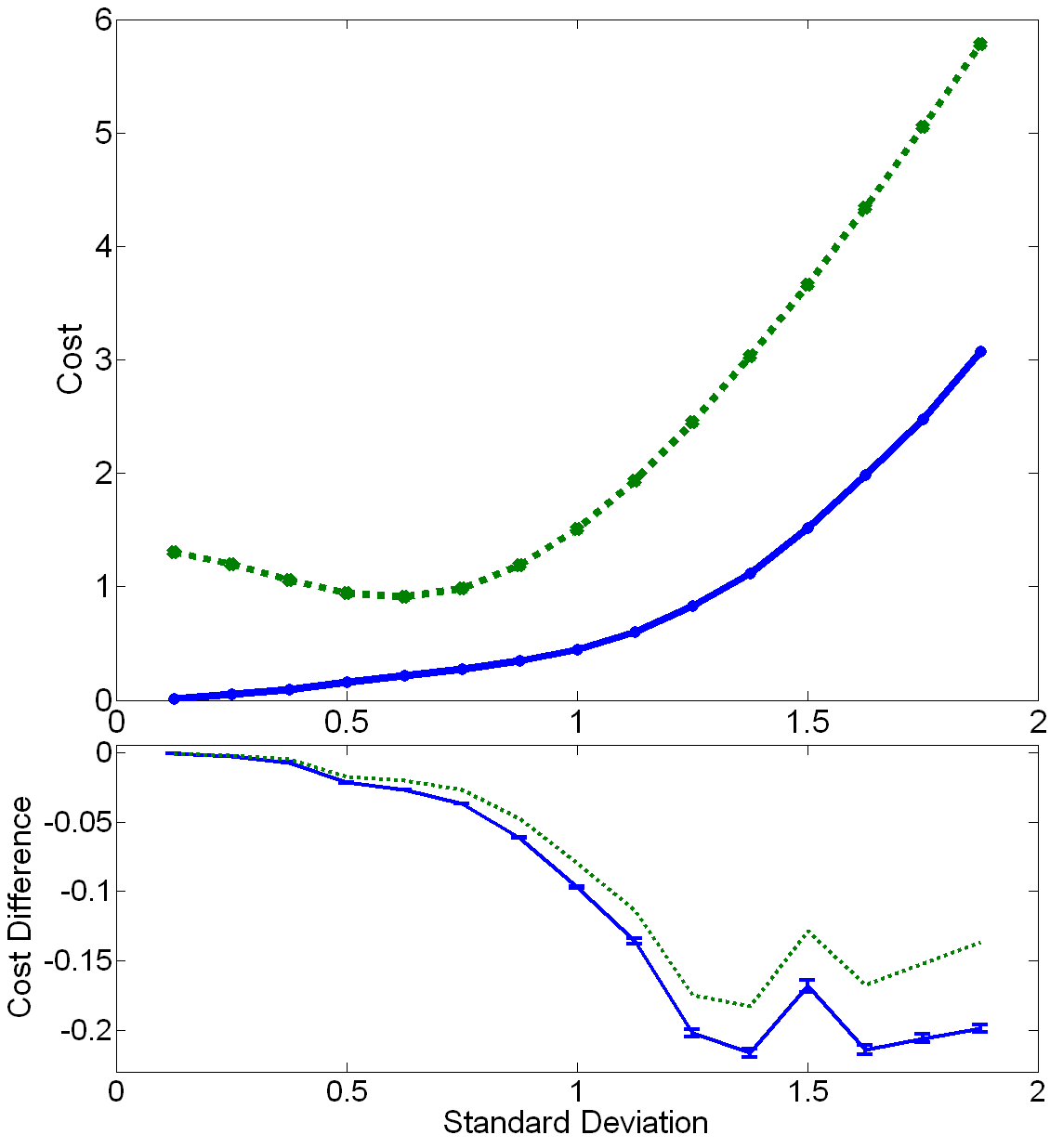
(a)  Two atoms

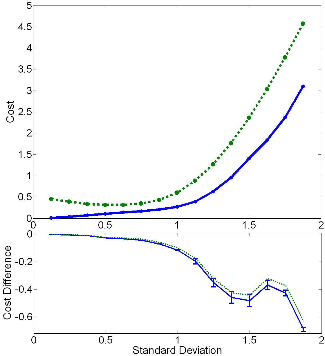
(b)  Four atoms

Figure 3: Comparison of the protocol derived in Ref. Bužek et al. (1999) and those derived by our method for two and four atoms and the cost function $C(\omega-f_{a})=(\omega-f_{a})^{2}$. SDP parameters are identical to those in Fig. 2. The plots are also as in Fig. 2, except that for this cost function, we can compute querier discretization errors $\epsilon_{q}$. Thus, the lower plots show $c_{l}-c_{u}$ as dotted lines above the line for $c_{l}-c_{u}-\epsilon_{q}$, which gives the lower bounds for the continuous problem.

Standard Deviation	$|0\rangle$	$|1\rangle$	$|2\rangle$
.25	.7071	0	.7071
.75	.5626	.6058	.5626
1.25	.5170	.6823	.5170
1.75	.5025	.7035	.5025
2.25	.5000	.7071	.5000

Table 1: Initial states that minimize the cost function $C(\omega-f_{a})=4\sin^{2}(\frac{\omega-f_{a}}{2})$ for one-query protocols assuming different width Gaussian priors. SDP parameters are identical to those of Fig. 2

For computing the graphs of Figs. 2 and 3, and the initial states in Table 1, we did not optimize the frequency estimates according to the iterative technique described at the end of Sect. IV.1. In order to achieve sufficiently small discretization error, we discretized the prior frequency distribution with $15$ points and used $20$ frequency estimates chosen by minimizing Eq. (16). The bounds are based on $100$ random discretizations to obtain sufficiently good statistics on the lower bound.

To verify the technique for obtaining error bounds, we compare our upper and lower bounds to the optimal solution obtained according to the formulas in Ref. Demkowicz-Dobrzanski (2011); this is illustrated in Fig. 4. We use the optimal set of classical frequency estimates derived in Ref. Demkowicz-Dobrzanski (2011); therefore, in the continuous limit, the clock SDP and that of Ref. Demkowicz-Dobrzanski (2011) should yield identical costs. Consequently, the deviation depicted in Fig. 4 is due entirely to discretization error and the limitations of our bounds.

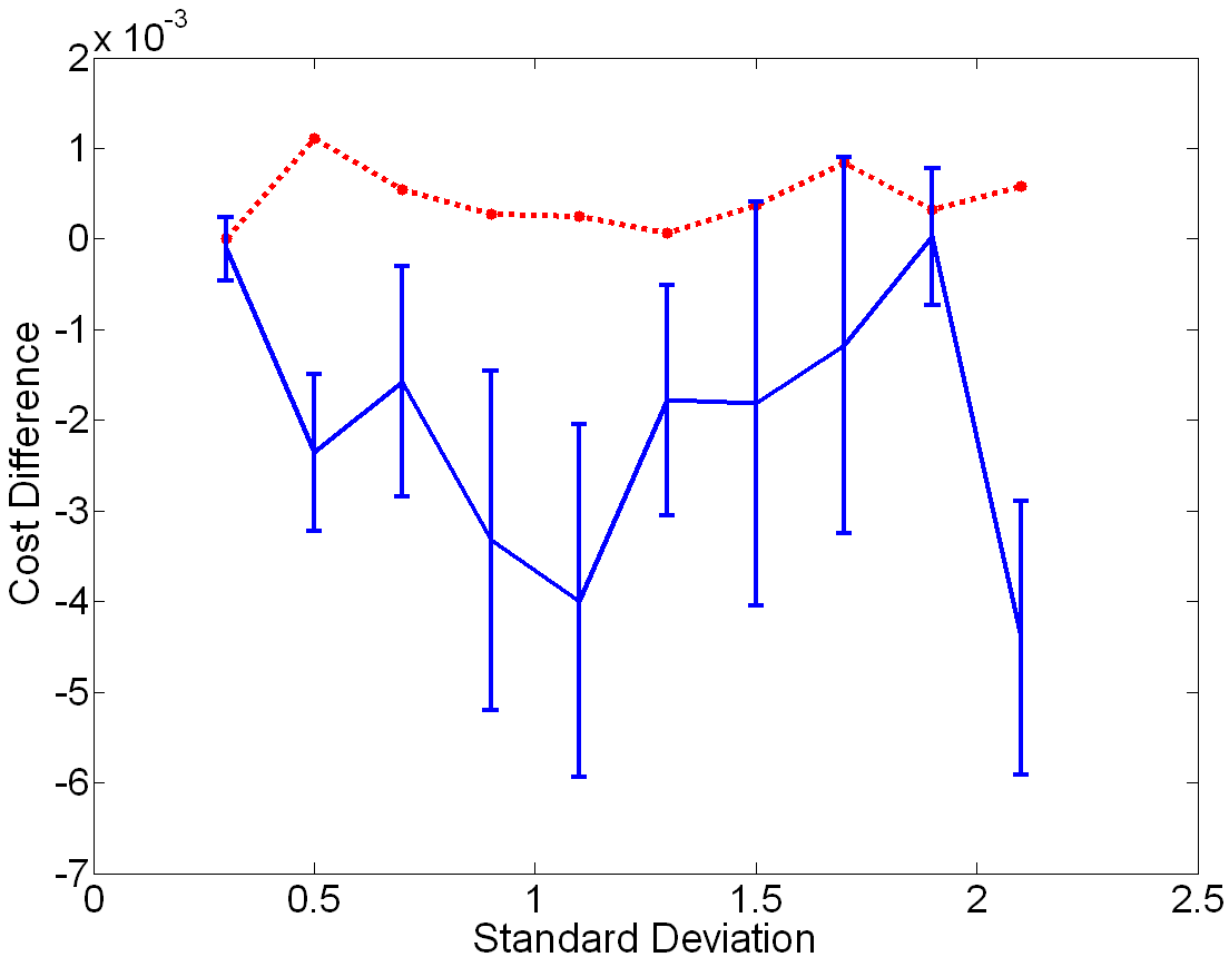
Figure 4: Comparison of the optimal protocol derived in Ref. Demkowicz-Dobrzanski (2011) and the one obtained by our SDP for two atoms. The dashed line depicts the difference between our upper bound and the cost computed in Ref. Demkowicz-Dobrzanski (2011), and the solid line depicts the difference between our lower bound and the cost computed in Ref. Demkowicz-Dobrzanski (2011). Error bars again correspond to the estimated standard error in the lower bound. We used a $15$-point prior discretization and set $F$ to the optimal set of frequency estimates derived in Demkowicz-Dobrzanski (2011), so there is no querier discretization error. The lower bound was computed by averaging 500 random oracle discretizations.

As discussed, our procedure can also optimize sequences of two or more clock queries ($t_{f}\geq 2$). If these queries are fully coherent, the algorithm is of the form given in Eq. (3), and the SDP implicitly optimizes the initial state, the $U(t_{i})$ and the measurement. Alternatively, we can combine the two queries classically. In this case we update our knowledge of the clock’s phase using Bayes’ rule between the queries. That is, after the first query, we compute posterior distributions for each measurement outcome, as in Eq. (17). We then run the SDP again, once for each outcome, using the corresponding posterior distribution as the new prior. We compute a new cost by averaging each of the costs obtained, weighted by the probability of obtaining the corresponding measurement outcome, $\mathrm{tr}(\sigma_{a})$. Here we assume that there is no noise between sequential queries. Any noise would affect the intermediate prior distributions. Fig. 5 compares these two methods for a sequence of two queries with two atoms. Here we used $|F|=25$ possible frequency estimates and the iterative technique described in Sect. IV.1 for optimizing them. We found that the number of frequency estimates needed was substantially reduced after optimization. For one query ($t_{f}=1$), and when such queries are combined classically, three estimates per query suffice after applying estimate optimization. When two queries are combined quantumly, five estimates suffice. It appears that, as expected, while we gain information by combining queries classically, fully coherent queries provide the greatest advantage. However, the technique developed for computing lower bounds cannot be applied to classical combinations of queries, so this advantage remains to be proven.

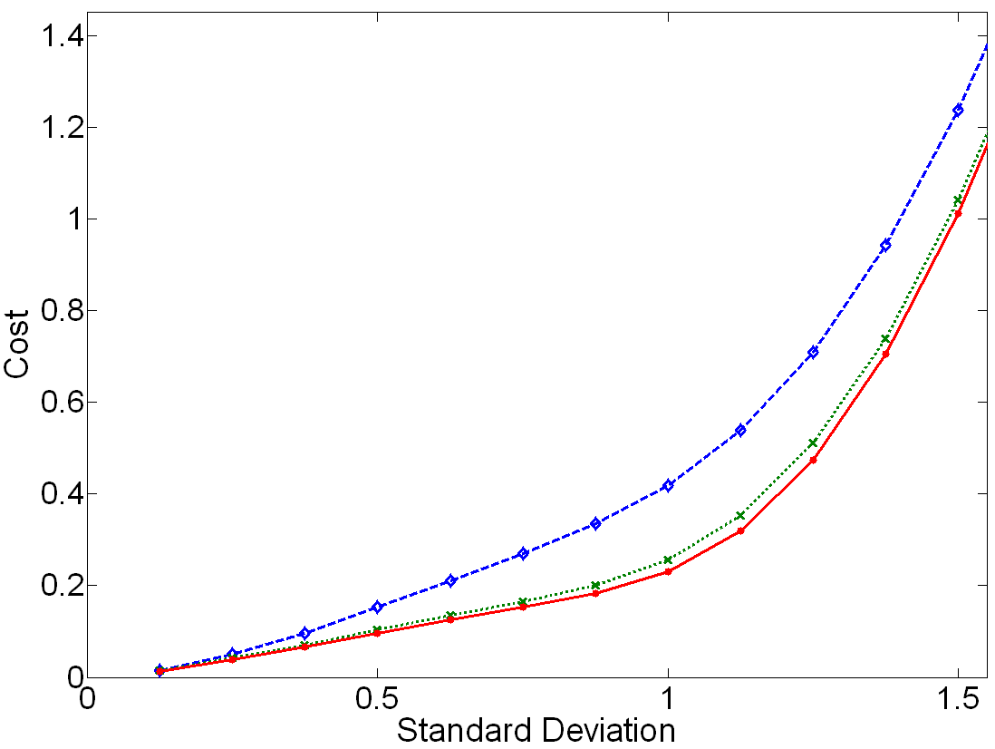
Figure 5: Average cost after one query (top, dashed line), two queries combined classically (middle, dotted line), and two coherent quantum queries (bottom, solid line). We used a $15$-point oracle discretization, $|F|=25$, the cost function $C(\omega-f_{a})=(\omega-f_{a})^{2}$, and simulated two atoms.

Table 2 examines the effect of adding more atoms to the clock. Additional atoms and additional queries always provide an advantage, as can be seen by reading down the table. The far right column gives the computational time required to run the SDP for a single discretization on a quad core $2.8\;\textrm{GHz}$ machine with $12\;\textrm{GiB}$ of RAM. Note that we are able to simulate more atoms than Table 2 may imply. For example, a simulation of $10$ atoms using a uniform $15$-point oracle discretization and $t_{f}=1$ was computed in 6 minutes, 3 seconds, and yields a cost of $0.0785$. Computing bounds for a system of this size, however, would require a great deal of computational time.

Number	Number	$c_{l}$	$c_{u}$	$s_{l}$	$\epsilon_{q}$	time
of Atoms	of Queries					(min:sec)
1	1	.6010	.6321	.0127	.0152	2:24
2	1	.4083	.4379	.0109	.0164	2:33
3	1	.2885	.3263	.0105	.0177	3:07
4	1	.1974	.2563	.0045	.0192	2:46
1	2	.4144	.4379	.0132	.0164	2:14
2	2	.1957	.2565	.0047	.0192	3:35
3	2	.1071	.2119	.0020	.0229	4:07
4	2	.0902	.2657	.0022	.0229	4:58

Table 2: Costs for various combinations of atoms and queries for a Gaussian prior with a standard deviation of $1$. SDP parameters are identical to those in Fig. 5. The times are given for solving one instance of the SDP. $100$ instances were solved for the estimates of $c_{l}$ and $c_{u}$.

Notice that on the far right of Fig. 3(b), and in the last two rows of Table 2, the gap between the lower bound and the upper bound becomes quite large. We need to increase the number of points in our discretizations if we wish to compute better approximations to the optimal solution for the continuous problem. This is as expected, since having more queries or atoms enables finer resolution of oracle frequencies. Fig. 6 illustrates the effect on our bounds of increasing the number of points in the oracle discretization. Here we are reanalyzing the last point in Fig. 3(b).

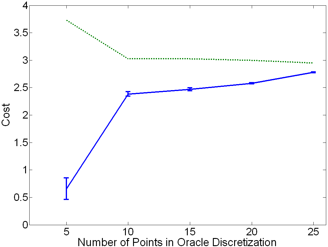
Figure 6: Upper ($c_{u}$, dotted line) and lower ($c_{l}$, solid line) bounds on cost for oracle discretizations with varying numbers of points. We are simulating the last point of Fig. 3(b) - that is, 4 atoms, a standard deviation of 1.875, and the quadratic cost function. The lower bound is computed by averaging 32 random oracle discretizations. Note that the values in Fig. 3 are for a $15$ point oracle discretization.

In summary, the method presented here is a general way of deriving better quantum clock protocols. Discretization is necessary, but the error introduced can be controlled. While the complexity of the SDPs to be solved limits the application of the method to small quantum systems, there are very promising atomic clocks, such as the ion-based ones, that use only a small number of atoms.

The optimization strategy pursued here is greedy, taking into account only the most recent prior. Therefore, it does not necessarily minimize long-term variance. Further research is required to develop more realistic strategies, taking advantage of knowledge of the clock’s history.

Finally, we note that the general form of the SDP and the discretization analysis given here can be used to extend the adversary method to continuous, noisy, and classical problems. It may also find applications to quantum parameter estimation problems other than phase or frequency estimation, where we wish to estimate the value of a parameter $x$ of an arbitrary but known family of unitary operators $U(x)$ that can be applied to quantum states of our choice.

Appendix A Remote State Preparation

Here we prove Thm. 1.

Proof.

Assume that we can remotely prepare $\{\sigma^{O}_{a}\}$ from $\rho^{OQ}$, and let $\{P_{a}^{Q}\}_{a}$ be the required POVM. Then $\sum_{a}\sigma^{O}_{a}=\sum_{a}\mathrm{tr}_{Q}P_{a}^{Q}\rho^{OQ}=\mathrm{tr}_{Q}(\sum_{a}P_{a})\rho^{OQ}=\rho^{O}$, by the definition of a POVM.

The converse is a generalization of the GHJW theorem Hughston et al. (1993) to mixed density operators. Suppose that $\sum_{a}\sigma_{a}^{O}=\rho^{O}$. To construct the required POVM, first write each $\sigma^{O}_{a}$ as an explicit mixture of pure states

$$\sigma_{a}^{O}=\sum_{m}p_{a,m}{|}{\psi_{am}}{\rangle}{\langle}{\psi_{am}}{|}.$$

By assumption, $\rho^{O}=\sum_{a,m}p_{a,m}{|}{\psi_{a,m}}{\rangle}{\langle}{\psi_{a,m}}{|}$. By filling in mixture terms with $p_{a,m}=0$ if necessary, we can assume that the range of the index $m$ is independent of $a$. Since $\rho^{OQ}={|}{\Phi}{\rangle}{\langle}{\Phi}{|}$ is pure, we can write the $OQ$ state in Schmidt form

$${|}{\Phi}{\rangle}=\sum_{j}\sqrt{q_{j}}{|}{\phi_{j}}{\rangle}{|}{\varphi_{j}}{\rangle},$$ (27)

where the ${|}{\phi_{j}}{\rangle}$ and ${|}{\varphi_{j}}{\rangle}$ are orthonormal in the Hilbert spaces of $O$ and $Q$, respectively. Thus $\rho^{O}$ can also be written as the mixture $\rho^{O}=\sum_{j}q_{j}{|}{\phi_{j}}{\rangle}{\langle}{\phi_{j}}{|}$. By unitary freedom (for example, see Nielsen and Chuang (2001), pg. 103),

$$\sqrt{p_{am}}{|}{\psi_{am}}{\rangle}=\sum_{j}u_{am,j}\sqrt{q_{j}}{|}{\phi_{j}}{\rangle},$$ (28)

where the $u_{am,j}$ are the entries of a unitary matrix. We can now define

$$P_{a}^{Q}=\sum_{m}\sum_{j,j^{\prime}}u_{am,j}^{*}u_{am,j^{\prime}}{|}{\varphi_{j}}{\rangle}{\langle}{\varphi_{j^{\prime}}}{|}.$$ (29)

That $\sum_{a}P_{a}={\mathchoice{\rm 1\mskip-4.0mul}{\rm 1\mskip-4.0mul}{\rm 1\mskip-4.5mul}{\rm 1\mskip-5.0mul}}$ follows from the unitarity condition for $u_{am,j}$. To verify the partial trace condition, compute

$$\mathrm{tr}_{Q}P_{a}^{Q}\rho^{OQ} = \sum_{m}\sum_{j,j^{\prime}}u_{am,j}^{*}u_{am,j^{\prime}}$$ (30)

$$\mathrm{tr}_{Q}\left({|}{\varphi_{j}}{\rangle}{\langle}{\varphi_{j^{\prime}}}{|}\sum_{l,l^{\prime}}\sqrt{q_{l}q_{l^{\prime}}}{|}{\phi_{l}}{\rangle}{\langle}{\phi_{l^{\prime}}}{|}{|}{\varphi_{l}}{\rangle}{\langle}{\varphi_{l^{\prime}}}{|}\right)$$

$$= \sum_{m}\sum_{j,j^{\prime}}u_{am,j}^{*}u_{am,j^{\prime}}\sqrt{q_{j}q_{j^{\prime}}}{|}{\phi_{j^{\prime}}}{\rangle}{\langle}{\phi_{j}}{|}$$

$$= \sum_{m}p_{am}{|}{\psi_{am}}{\rangle}{\langle}{\psi_{am}}{|}$$

$$= \sigma_{a}^{O},$$

as desired. ∎

Appendix B Querier Discretization Bound

Here is the proof of Thm. 3.

Proof.

Define $C(p,{\cal Q})=\sum_{a}\int C(\omega-g_{a})p(g_{a},\omega|{\cal Q})d\omega$, where the $g_{a}$ are ${\cal Q}$’s frequency estimates. Then $C(p,{\cal Q})$ is the expected cost of ${\cal Q}$ given prior $p$. Let $g(a)$ be defined by

$$g(a)=\mathrm{argmin}_{g}\left(\int C(\omega-g)p(a|\omega,{\cal Q})p(\omega)d\omega\right).$$ (31)

Then $g(a)$ is the optimum frequency estimate ${\cal Q}$ could make given measurement outcome $a$. Let ${\cal Q}_{g}$ be ${\cal Q}$ modified to make the frequency estimates $g(a)$.

Let $B$ be the expression on the right-hand-side of Eq. (16). We show that $C(p,{\cal Q}_{g})\geq S_{C}(p,F)-B$ for any algorithm ${\cal Q}$. Since $S_{C}(p,\mathbb{R})=\inf_{{\cal Q}}C(p,{\cal Q})=\inf_{\cal Q}C(p,{\cal Q}_{g})$, the result follows. We prove the bound in two steps. In the first step we force the frequency estimates to lie in $[f_{1},f_{N}]$ and in the second we change them to lie in $F$.

For the first step, let $\tilde{g}(a)$ be the value in $[f_{1},f_{N}]$ nearest to $g(a)$. If $\tilde{g}(a)=g(a)$, then $C(\omega-g(a))\geq C(\omega-\tilde{g}(a))-M(\omega)$ since $M(\omega)\geq 0$. If $\tilde{g}(a)=f_{1}$, then one of the following holds: 1. $\omega\geq f_{1}$, in which case $\tilde{g}(a)$ is nearer $\omega$ and on the same side, so that $C(\omega-g(a))\geq C(\omega-\tilde{g}(a))\geq C(\omega-\tilde{g}(a))-M(\omega)$. 2. $\omega<f_{1}$, in which case $C(\omega-g(a))\geq 0=C(\omega-f_{1})-C(\omega-f_{1})=C(\omega-\tilde{g}(a))-M(\omega)$. A similar argument works for $\tilde{g}(a)=f_{N}$. Substituting the inequalities in the integral for $C(p,{\cal Q})$ we get

$$C(p,{\cal Q}_{g}) \geq \sum_{a}\int C(\omega-\tilde{g}(a))p(a|\omega,{\cal Q})p(\omega)d\omega$$ (32)

$${}-\sum_{a}\int M(\omega)p(a|\omega,{\cal Q})p(\omega)d\omega$$

$$= C(p,{\cal Q}_{\tilde{g}})-\int M(\omega)d\omega.$$

For the second step, we modify $Q_{\tilde{g}}$ to $Q_{\tilde{f}}$, where $\tilde{f}(a)$ is one of the elements of $F$ on either side of $\tilde{g}(a)$. That is, because $f_{1}\leq\tilde{g}(a)\leq f_{N}$, there exists a unique $j$ such that $f_{j}\leq\tilde{g}(a)\leq f_{j+1}$, and we set $\tilde{f}(a)$ to either $f_{j}$ or $f_{j+1}$. Define $\lambda\in[0,1]$ by $\tilde{g}(a)=\lambda f_{j}+(1-\lambda)f_{j+1}$. It is convenient to let $Q_{\tilde{f}}$ be a “mixed” (randomized) algorithm, where $\tilde{f}(a)=f_{j}$ with probability $\lambda$ and $f_{j+1}$ with probability $1-\lambda$. Note that a mixed algorithm of this sort cannot be better than the optimal one, that is $C(p,Q_{\tilde{f}})\geq S_{C}(p,F)$. To bound the cost, we consider a given $a$ and $\omega$ and estimate the quantity

$$c(\omega,a) = \lambda C(w-f_{j})+(1-\lambda)C(w-f_{j+1})$$

$${}-C(\omega-\tilde{g}(a))$$

$$= \lambda\left(C(w-f_{j})-C(\omega-\tilde{g}(a))\right)$$

$${}+(1-\lambda)\left(C(w-f_{j+1})-C(\omega-\tilde{g}(a))\right).$$

Define $\omega_{0}=\omega-\tilde{g}(a)$, $\omega_{l}=\omega-f_{j+1}$ and $\omega_{u}=\omega-f_{j}$. We can estimate

$$C(\omega)-C(\omega_{0}) = (\omega-\omega_{0})C^{\prime}(\omega_{0})$$

$${}+\int_{0}^{\omega-\omega_{0}}\int_{0}^{x}C^{\prime\prime}(\omega_{0}+y)dydx$$

$$\leq (\omega-\omega_{0})C^{\prime}(\omega_{0})$$

$${}+\frac{1}{2}(\omega-\omega_{0})^{2}\max_{y}C^{\prime\prime}(y)$$

$$\leq (\omega-\omega_{0})C^{\prime}(\omega_{0})+\frac{b}{2}(\omega-\omega_{0})^{2}.$$

Substituting this bound for each summand of Eq. (LABEL:eq:c_omega_a) gives

$$c(\omega,a) \leq \lambda((\omega_{u}-\omega_{0})C^{\prime}(\omega_{0})+\frac{b}{2}(\omega_{u}-\omega_{0})^{2})$$ (35)

$${}+(1-\lambda)((\omega_{l}-\omega_{0})C^{\prime}(\omega_{0})+\frac{b}{2}(\omega_{l}-\omega_{0})^{2})$$

$$= \frac{b}{2}\left(\lambda(\omega_{u}-\omega_{0})^{2}+(1-\lambda)(\omega_{l}-\omega_{0})^{2})\right)$$

$$= \frac{b}{2}\left(\lambda(\omega_{u}-\omega_{0})(\omega_{u}-\omega_{l})\right)$$

$$\leq \frac{b}{2}\frac{(f_{j+1}-f_{j})^{2}}{4},$$

where we first applied $\lambda\omega_{u}+(1-\lambda)\omega_{l}=\omega_{0}$. The next identity requires applying $(1-\lambda)(\omega_{l}-\omega_{0})=-\lambda(\omega_{u}-\omega_{0})$ to the second summand, and the final inequality is obtained by noting that $\lambda(\omega_{u}-\omega_{0})/(f_{j+1}-f_{j})$ is maximized at $\lambda=1/2$. We can apply the above inequalities to bound $C(p,{\cal Q}_{\tilde{g}})$ as follows:

$$C(p,{\cal Q}_{\tilde{g}}) = \sum_{a}\int C(\omega-\tilde{g}(a))p(a|\omega,{\cal Q})p(\omega)d\omega$$ (36)

$$\geq \sum_{a}\int\big{(}\lambda C(\omega-f_{j})+(1-\lambda)C(\omega-f_{j+1})$$

$${}-\max_{j}\frac{b}{8}(f_{j+1}-f_{j})^{2}\big{)}p(a|\omega,{\cal Q})p(\omega)d\omega$$

$$= C(p,{\cal Q}_{\tilde{f}})-\max_{j}\frac{b}{8}(f_{j+1}-f_{j})^{2}$$

$$\geq S_{C}(p,F)-\max_{j}\frac{b}{8}(f_{j+1}-f_{j})^{2}.$$

To finish the proof, we combine Eqs. (32) and (36). ∎