Interpolatory $\mathcal{H}_{\infty}$ Model Reduction

Abstract

We introduce an interpolation framework for $\mathcal{H}_{\infty}$ model reduction founded on ideas originating in optimal-$\mathcal{H}_{2}$ interpolatory model reduction, realization theory, and complex Chebyshev approximation. By employing a Loewner “data-driven” framework within each optimization cycle, large-scale $\mathcal{H}_{\infty}$ norm calculations can be completely avoided. Thus, we are able to formulate a method that remains effective in large-scale settings with the main cost dominated by sparse linear solves. Several numerical examples illustrate that our approach will produce high fidelity reduced models consistently exhibiting better $\mathcal{H}_{\infty}$ performance than those produced by balanced truncation; these models often are as good as (and occasionally better than) those models produced by optimal Hankel norm approximation. In all cases, these reduced models are produced at far lower cost than is possible either with balanced truncation or optimal Hankel norm approximation.

1 Introduction

The need for high accuracy mathematical models in problems involving simulation and control often results in dynamical systems described by a large number of differential equations. Working with such large-scale systems can easily place overwhelming demands on computational resources, a problem which model reduction methods seek to alleviate by approximating the original model with another model consisting of far fewer (but carefully crafted) differential equations. Strategies for carrying out this approximation should be both efficient and accurate. For an overview of model reduction, see [1].

We consider here single-input/single-output (SISO) linear dynamical systems given in state-space form as:

$$\bm{E}\dot{\bm{x}}(t)=\bm{A}\bm{x}(t)+\bm{b}\,u(t),\qquad y(t)=\bm{c}^{T}\,\bm{x}(t)+d\,u(t),$$ (1)

where $\bm{E},\,\bm{A}\in\mbox{\Bb R}^{n\times n}$, $\bm{b},\bm{c}\in\mbox{\Bb R}^{n}$ and $d\in\mbox{\Bb R}$. $\bm{E}$ is assumed to be nonsingular throughout, although our approach extends without difficulty to cases where $\bm{E}$ is singular so long as $\mbox{{nullity}}(\bm{E})=\mbox{{nullity}}(\bm{E}^{2})$ (that is, provided that $0$ is a nondefective eigenvalue for $\bm{E}$). $\bm{x}(t)\in\mbox{\Bb R}^{n}$ are the states; $u(t)\in\mbox{\Bb R}$ is the input; and $y(t)\in\mbox{\Bb R}$ is the output of the dynamical system in (1). The transfer function of the system is

$$H(s)=\bm{c}^{T}(s\bm{E}-\bm{A})^{-1}\bm{b}+d,$$

defined for $s\in\mbox{\Bb C}$. In accord with standard convention, we denote both the system and its transfer function by $H(s)$. We assume that $H(s)$ is both controllable and observable. The order of $H(s)$ is the number of poles it possesses, counting multiplicity. Since $\bm{E}$ is nonsingular, all poles of $H(s)$ are finite and since $H(s)$ is both controllable and observable, the order of $H(s)$ is identical to the dimension, $n$, of the state vector $\bm{x}$ in (1).

We denote by $\mathcal{H}_{\infty}^{k}$, the set of rational functions of order at most $k$ which are bounded and analytic in the closed right half plane in $\mathbb{C}$. We assume in all that follows that $H\in\mathcal{H}_{\infty}^{n}$. The $\mathcal{H}_{\infty}$ norm of $H$ is defined as

$$\left\|H\right\|_{\mathcal{H}_{\infty}}=\max_{\omega\in{\mathbb{R}}}\mid H(\jmath\omega)\mid.$$ (2)

If the input function, $u(t)$, is square integrable: $\displaystyle\|u\|_{L^{2}}=\left(\int_{0}^{\infty}\mid u(t)\mid^{2}\,dt\right)^{\frac{1}{2}}<\infty$, then the output function, $y(t)$, of (1) will be square integrable as well; $u$ and $y$ have Fourier transforms $\widehat{u},\,\widehat{y}\in L^{2}(\mbox{\Bb R})$ that are related according to $\widehat{y}(\omega)=H(\jmath\omega)\widehat{u}(\omega)$. One immediately observes that the $\mathcal{H}_{\infty}$ norm defined in (2) is an $L^{2}$-induced operator norm of the underlying convolution operator mapping $u\mapsto y$.

Our goal is to construct another system

$$\bm{E}_{r}\dot{\bm{x}}_{r}(t)=\bm{A}_{r}\bm{x}_{r}(t)+\bm{b}_{r}u(t),\qquad y_{r}(t)=\bm{c}_{r}^{T}\bm{x}_{r}(t)+d_{r}u(t)$$ (3)

of much smaller order $r\ll n$, with $\bm{E}_{r},\,\bm{A}_{r}\in\mbox{\Bb R}^{r\times r}$, $\bm{b}_{r},\,\bm{c}_{r}\in\mbox{\Bb R}^{r}$, and $d_{r}\in\mbox{\Bb R}$ determined so that $y_{r}$ approximates $y$ uniformly well over all $u\in L^{2}(\mbox{\Bb R}^{+})$, in an appropriate sense.

Toward this end, define a reduced transfer function associated with (3) as $H_{r}(s)=\bm{c}_{r}^{T}(s\bm{E}_{r}-\bm{A}_{r})^{-1}\bm{b}_{r}+d_{r}$. Then, for any $u\in L^{2}(\mbox{\Bb R}^{+})$,

$$\|y-y_{r}\|_{L^{2}}\leq\|H-H_{r}\|_{\mathcal{H}_{\infty}}\|u\|_{L^{2}}.$$ (4)

The error transfer function, $H(s)-H_{r}(s)$, may be rewritten as

$$H(s)-H_{r}(s)=\bm{c}^{T}(s\bm{E}-\bm{A})^{-1}\bm{b}-\left[\bm{c}_{r}^{T}(s\bm{E}_{r}-\bm{A}_{r})^{-1}\bm{b}_{r}+(d_{r}-d)\right].$$

Evidently, a non-zero $d$-term in the original model may be absorbed into a reduced-order model by assigning $d_{r}\mapsto(d_{r}-d)$. This allows us to assume in all that follows that $d=0$ in the original model without any loss of generality.

In view of (4), the output error magnitude, $\|y-y_{r}\|_{L^{2}}$, may be made uniformly small over all bounded inputs $u$ (say, with $\|u\|_{L^{2}}\leq 1$) if we find a reduced system, $H_{r}$, that makes $\|H-H_{r}\|_{\mathcal{H}_{\infty}}$ small. This leads naturally to the optimal $\mathcal{H}_{\infty}$ model reduction problem:

For a given $H\in\mathcal{H}_{\infty}^{n}$ and reduction order $r<n$, find $H_{r}^{\star}\in\mathcal{H}_{\infty}^{r}$, that solves

$$\min\limits_{\hat{H}_{r}\in\mathcal{H}_{\infty}^{r}}\left\|H-\hat{H}_{r}\right\|_{\mathcal{H}_{\infty}}.$$ (5)

This problem is an active area of research [2]. We develop a methodology for approximating solutions to (5) that remain effective in large-scale settings, settings where the original state-space dimension, $n$, could be on the order of $10^{5}$ or more, for example. Most methods known to us will be intractable even for modest system order, say, on the order of a few thousand (with the exception of balanced truncation, see the discussion below).

Kavranoğlu and Bettayeb [26] showed that (5) can be converted into an optimal Hankel norm approximation problem for a special imbedded system with augmented input and output mappings. However, this approach is infeasible in practice since knowledge both of the minimum of (5) as well the imbedded system is required. As noted in [26], this information is available (or computationally accessible) only in very special cases.

Several methods to solve (5) that utilize linear matrix inequality (LMI) frameworks have been presented as well; see, for example, [15, 25, 24, 23, 41] and references therein. These approaches rapidly become computationally intractable with increasing state space dimension. Indeed, published examples illustrating LMI-based methods in [15, 25, 24, 23, 41] all had order less than $n=10$.

The most common practical methods for obtaining satisfactory $\mathcal{H}_{\infty}$ reduced models are Gramian-based methods such as balanced truncation (BT) [31, 32] and optimal Hankel norm approximation methods (HNA) [14]. Both approaches are known to yield small approximation errors in the $\mathcal{H}_{\infty}$ norm [19, 1], though neither generally is capable of producing globally optimal solutions to (5). Both approaches also remain computationally feasible for modest state space dimension (perhaps a few thousand), but significantly larger state space dimension still presents challenges. HNA requires an all-pass dilation of the full-order model followed by a full eigenvalue decomposition. These are dense matrix operations, having a complexity growing with $\mathcal{O}(n^{3})$, which generally limits problem sizes to a few thousand. Notably, [11] was able to extend HNA to dynamical systems having state space dimension of $\mathcal{O}(10^{4})$, using state-of-the-art numerical techniques tailored to high performance computer architectures.

The situation for BT is a bit better. BT has been applied to systems of order $\mathcal{O}(10^{5})$ by solving the underlying Lyapunov equations iteratively using ADI-type algorithms; see, for example, [20, 38, 33, 10, 35, 22] and references therein.

We describe here a different model reduction methodology that can be applied effectively even for very large state space dimension, yielding reduced models typically having smaller $\mathcal{H}_{\infty}$ errors than either BT or HNA  moreover, at significantly lower cost. Towards this end, we present a new framework for the $\mathcal{H}_{\infty}$ approximation problem using interpolatory model reduction. By connecting ideas from interpolatory $\mathcal{H}_{2}$ model reduction [21], realization theory [29], and complex Chebyshev approximation [39], we develop an interpolation-based method for $\mathcal{H}_{\infty}$-approximation that remains numerically efficient in large-scale settings. The main cost of our approach involves the solution of sparse linear systems. We demonstrate that our approach can yield reduced-order systems having $\mathcal{H}_{\infty}$ errors which are often half that of BT, and very close to (indeed, sometimes better than) that of HNA. For symmetric systems, our method typically produces reduced-order systems with $\mathcal{H}_{\infty}$-errors that are near the theoretical best possible of (5).

The rest of the paper is organized as follows: we close this section with a brief review of interpolatory model reduction and related approaches for solving the optimal $\mathcal{H}_{2}$ approximation problem. We introduce our method in §2 and illustrate its effectiveness via several numerical examples in §3.

Interpolatory model reduction.

Given a dynamical system $H(s)$ and a set of points $\{s_{1},\,s_{2},\,\ldots,\,s_{k}\}\subset\mbox{\Bb C}$, interpolatory model reduction produces a dynamical system $H_{r}(s)$ such that $H_{r}(s)$ interpolates $H(s)$ together with a prescribed number of derivatives at the points $\{s_{1},\,s_{2},\,\ldots,\,s_{k}\}$. Although this is posed as a rational interpolation problem, the construction of a solution may be accomplished with a variety of rational Krylov subspace projection techniques. Rational interpolation via projection was first proposed by Skelton et al. [42, 44, 45]. Later, Grimme [16] showed how to construct a reduced-order (Hermite) interpolant using a method of Ruhe.

Theorem 1.1 (Grimme [16]).

Given $H(s)=\bm{c}^{T}(s\bm{E}-\bm{A})^{-1}\bm{b}$ and a point-set $\mathcal{S}_{1}\subset\mathbb{C}$ containing $r$ distinct points: $\mathcal{S}_{1}=\{s_{1},\ldots,s_{r}\}$, let

$$\bm{V}_{r}=[(s_{1}\bm{E}-\bm{A})^{-1}\bm{b}\dots(s_{r}\bm{E}-\bm{A})^{-1}\bm{b}]\qquad\bm{W}_{r}^{T}=\begin{bmatrix}\bm{c}^{T}(s_{1}\bm{E}-\bm{A})^{-1}\\ \vdots\\ \bm{c}^{T}(s_{r}\bm{E}-\bm{A})^{-1}\end{bmatrix}.$$ (6)

Define a reduced-order model $H_{r}^{0}(s)=\bm{c}_{r}^{T}(s\bm{E}_{r}-\bm{A}_{r})^{-1}\bm{b}_{r}$, where $d_{r}=0$ and

$$\bm{E}_{r}=\bm{W}_{r}^{T}\bm{E}\bm{V}_{r},~{}~{}\bm{A}_{r}=\bm{W}_{r}^{T}\bm{AV}_{r},~{}~{}\bm{b}_{r}=\bm{W}_{r}^{T}\bm{b},~{}~{}{\rm and}~{}~{}\bm{c}_{r}^{T}=\bm{c}^{T}\bm{V}_{r}.$$ (7)

Then $H(s_{i})=H_{r}^{0}(s_{i})$ and $H^{\prime}(s_{k})=H_{r}^{0\,\prime}(s_{k})$, for $i=1,\dots 2r$ where $\phantom{}{}^{\prime}$ denotes the derivative with respect to the frequency parameter, $s$.

Higher-order derivatives can be matched similarly; for details, see [16, 4].

$\mathcal{H}_{2}$-optimality conditions.

Theorem 1.1 gives explicitly computable conditions that will yield a reduced-order model satisfying $2r$ interpolation conditions; one need only solve $2r$ linear algebraic systems to form the columns of $\bm{V}_{r}$ and $\bm{W}_{r}$. Notably, Theorem 1.1 carries no hint of how best to choose these interpolation points. A method for determining interpolation points that leads to reduced-order models that are (locally) optimal with respect to the $\mathcal{H}_{2}$ error was developed in [21] and will be a point of departure for the approach we propose here.

For a SISO dynamical system $H(s)$, the $\mathcal{H}_{2}$ norm is defined as

$$\left\|H\right\|_{\mathcal{H}_{2}}=\left(\frac{1}{2\pi}\int_{-\infty}^{\infty}\mid H(\jmath\omega)\mid^{2}d\omega\right)^{1/2}.$$ (8)

Then, for a given full-order model $H(s)$, and selected reduction order $r<n$, the optimal $\mathcal{H}_{2}$ approximation problem seeks a reduced model, ${\displaystyle H_{r}^{0}(s)}$, that solves

$$\min\limits_{\hat{H}_{r}^{0}\in\mathcal{H}_{2}^{r}}\left\|H-\hat{H}_{r}^{0}\right\|_{\mathcal{H}_{2}}.$$ (9)

The approximation problem (9) has been studied extensively; see, for example, [30],[43],[21], [36], [40], [17], [6], [7],[47] and references therein. First-order necessary conditions for $\mathcal{H}_{2}$-optimal approximation may be formulated in terms of interpolation conditions:

Theorem 1.2 ([30, 21]).

Given a full-order model $H(s)$, let $H_{r}^{0}(s)$ be an $\mathcal{H}_{2}$-optimal reduced order model of order $r$, with simple poles $\hat{\lambda}_{1},\dots,\hat{\lambda}_{r}$. Then,

$$H(-\hat{\lambda}_{i})=H_{r}^{0}(-\hat{\lambda}_{i})~{}~{}~{}{\rm and}~{}~{}~{}H^{\prime}(-\hat{\lambda}_{i})=H_{r}^{0\,\prime}(-\hat{\lambda}_{i})~{}~{}~{}{\rm for}~{}~{}~{}i=1,\dots,r,$$ (10)

where $\phantom{}{}^{\prime}$ denotes differentiation with respect to the frequency parameter, $s$.

These necessary conditions characterize the $\mathcal{H}_{2}$-optimal reduced order model as a rational Hermite interpolant matching the full-order transfer function and its derivative at mirror images of the reduced-order system poles. This can be accomplished with the help of Theorem 1.1 once the poles of $H_{r}^{0}(s)$ are known. Of course, the poles of $H_{r}^{0}(s)$ are not known a priori, but they can be computed iteratively using the Iterative Rational Krylov Algorithm (IRKA) developed by Gugercin et al. [21].

Algorithm IRKA. Iterative Rational Krylov Algorithm [21] Given a full-order $H(s)$, a reduction order $r$, and convergence tolerance $\mathsf{tol}$. 1. Make an initial selection of interpolation points $s_{i}$, for $i=1,\dots,r$ that is closed under complex conjugation. 2. Construct $\bm{V}_{r}$ and $\bm{W}_{r}$ as in (6) with $s_{i+r}=s_{i}$ for $i=1,\ldots,\,r$ 3. while (relative change in $\{s_{i}\}<\mathsf{tol}$) a) $\bm{E}_{r}=\bm{W}_{r}^{T}\bm{E}\bm{V}_{r}$ and $\bm{A}_{r}=\bm{W}_{r}^{T}\bm{A}\bm{V}_{r}$ b) Solve $r\times r$ eigenvalue problem $\bm{A}_{r}\mathbf{u}=\lambda\bm{E}_{r}\mathbf{u}$. c) Assign $s_{i}=s_{i+r}\leftarrow-\lambda_{i}(\bm{A}_{r},\bm{E}_{r})$ for $i=1,\dots,r$. d) Update $\bm{V}_{r}$ and $\bm{W}_{r}$  as in (6) using new $\{s_{i}\}$. 4. $\bm{E}_{r}=\bm{W}_{r}^{T}\bm{E}\bm{V}_{r}$, $\bm{A}_{r}=\bm{W}_{r}^{T}\bm{A}\bm{V}_{r}$, $\bm{b}_{r}=\bm{W}_{r}^{T}\bm{b}$, $\bm{c}_{r}^{T}=\bm{c}^{T}\bm{V}_{r}$, and $d_{r}=0$.

IRKA is a fixed point iteration that in the SISO case typically exhibits rapid convergence to a local minimizer of the $\mathcal{H}_{2}$-optimal model reduction problem. Sparsity in $\bm{E}$ and $\bm{A}$ can be well-exploited in the linear solves of Steps 2 and 3c and IRKA has been remarkably successful in producing high fidelity reduced-order approximations in large-scale settings; it has been applied successfully in finding $\mathcal{H}_{2}$-optimal reduced models for systems of high order (e.g., $n>160,000$, see [27]). For details on the algorithm, we refer to the original source [21].

2 An interpolatory approach for $\mathcal{H}_{\infty}$ approximation

The principal result that defines the character of our approach was provided by Trefethen in [39]; it is an analog to the Chebyshev Equioscillation Theorem.

Theorem 2.1 (Trefethen [39]).

Suppose $H(s)$ is a transfer function associated with a dynamical system as in (1). Let $H_{r}^{\rm opt}(s)$ be an optimal $\mathcal{H}_{\infty}$ approximation to $H(s)$ (i.e., a solution to (5) ) and let $H_{r}(s)$  be any $r^{\rm th}$ order stable approximation to $H(s)$ that interpolates $H(s)$ at $2r+1$ points in the open right half plane. Then

$$\min_{\omega\in\mbox{\Bb R}}|H(\jmath\omega)-H_{r}(\jmath\omega)|\leq\|H-H_{r}^{\rm opt}\|_{\mathcal{H}_{\infty}}\leq\|H-H_{r}\|_{\mathcal{H}_{\infty}}$$

In particular, if $|H(\jmath\omega)-H_{r}(\jmath\omega)|=\mathsf{const}$ for all $\omega\in\mbox{\Bb R}$ then $H_{r}(s)$ is itself an optimal $\mathcal{H}_{\infty}$ approximation to $H(s)$.

One sees from this that a good $\mathcal{H}_{\infty}$ approximation will be obtained when the modulus of the error, $|H(s)-H_{r}(s)|$, is nearly constant as $s=\jmath\omega$ runs along the imaginary axis. We select $2r+1$ interpolation points in the open right half plane that will induce this. By utilizing Theorem 1.1, we may locate $2r$ interpolation points in the right half plane as we like, producing an interpolating reduced-order system, $H_{r}^{0}(s)$. Also, $H(\infty)=H_{r}^{0}(\infty)=0$ so we can exploit the freedom in choosing $d_{r}$ to move the $(2r+1)^{\rm st}$ interpolation point from $\infty$ into the open right half-plane. Note that the straightforward construction, $H_{r}(s,d_{r})=H_{r}^{0}(s)+d_{r}$, creates a reduced-order model that has all interpolation points depending on $d_{r}$. We prefer a different formulation that uncouples the $2r$ interpolation points associated with $H_{r}^{0}(s)$ from the influence of $d_{r}$. The construction that accomplishes this was introduced in [29] (see also [5] for a formulation close to what we use here).

Theorem 2.2.

Given $H(s)=\bm{c}^{T}(s\bm{I}-\bm{A})^{-1}\bm{b}$ and a point-set $\mathcal{S}\ \subset\mathbb{C}$ containing $r$ distinct points: $\mathcal{S}=\{s_{1},\ldots,s_{r}\}$, let $\bm{V}_{r}$, $\bm{W}_{r}$, $\bm{E}_{r}$, $\bm{A}_{r}$, $\bm{b}_{r}$, and $\bm{c}_{r}$ be defined as in Theorem 1.1. For any given $d_{r}\in\mbox{\Bb R}$, define a new reduced-order system

$$H_{r}(s,d_{r})=(\bm{c}_{r}-d_{r}\bm{e})^{T}(s\bm{E}_{r}-\bm{A}_{r}-d_{r}\bm{e}\bm{e}^{T})^{-1}(\bm{b}_{r}-d_{r}\bm{e})+d_{r}$$ (11)

where $\bm{e}$ denotes a vector of ones. Define auxiliary reduced systems:

$$H_{r}^{0}(s)=\bm{c}_{r}^{T}(s\bm{E}_{r}-\bm{A}_{r})^{-1}\bm{b}_{r},\quad \quad G_{1}(s)=\bm{e}^{T}(s\bm{E}_{r}-\bm{A}_{r})^{-1}\bm{b}_{r},$$

$$G_{2}(s)=\bm{c}_{r}^{T}(s\bm{E}_{r}-\bm{A}_{r})^{-1}\bm{e},\quad\mbox{and} \qquad G_{3}(s)=\bm{e}^{T}(s\bm{E}_{r}-\bm{A}_{r})^{-1}\bm{e}.$$

Then

$$H_{r}(s,d_{r})=H_{r}^{0}(s)+d_{r}\frac{(G_{1}(s)-1)(G_{2}(s)-1)}{1-d_{r}G_{3}(s)}$$ (12)

and for all $d_{r}\in\mbox{\Bb R}$

$$H(s_{i})=H_{r}^{0}(s_{i})=H_{r}(s_{i},d_{r})~{}~{}\mbox{ and }~{}~{}H^{\prime}(s_{i})=H_{r}^{0\,\prime}(s_{i})=H_{r}^{\prime}(s_{i},d_{r})\quad\mbox{ for }\quad i=1,\ldots,r$$

where $\phantom{}{}^{\prime}$ denotes the derivative with respect to the frequency parameter, $s$.

Proof: The expression (12) follows from (11) with straightforward manipulations that begin with the Sherman-Morrison formula:

$$(s\bm{E}_{r}-\bm{A}_{r}-d_{r}\bm{e}\bm{e}^{T})^{-1}=(s\bm{E}_{r}-\bm{A}_{r})^{-1}+\frac{d_{r}}{1-d_{r}G_{3}(s)}(s\bm{E}_{r}-\bm{A}_{r})^{-1}\bm{e}\bm{e}^{T}(s\bm{E}_{r}-\bm{A}_{r})^{-1}$$

Define $\bm{P}(s)=\bm{V}_{r}(s\bm{E}_{r}-\bm{A}_{r})^{-1}\bm{W}_{r}^{T}(s\bm{E}-\bm{A})$. Observe that $\bm{P}(s)$ is a (skew) projection onto $\mbox{{Ran}}(\bm{V}_{r})$ for any $s\in\mbox{\Bb C}$ for which it is well-defined and so we have

$$\bm{V}_{r}\bm{e}_{k}= \bm{P}(s_{k})\bm{V}_{r}\bm{e}_{k}=\left[\bm{V}_{r}(s_{k}\bm{E}_{r}-\bm{A}_{r})^{-1}\bm{W}_{r}^{T}(s_{k}\bm{E}-\bm{A})\right](s_{k}\bm{E}-\bm{A})^{-1}\bm{b}$$

$$=\bm{V}_{r}(s_{k}\bm{E}_{r}-\bm{A}_{r})^{-1}\bm{W}_{r}^{T}\bm{b}=\bm{V}_{r}(s_{k}\bm{E}_{r}-\bm{A}_{r})^{-1}\bm{b}_{r}$$

Linear independence of the columns of $\bm{V}_{r}$ then implies $\bm{e}_{k}=(s_{k}\bm{E}_{r}-\bm{A}_{r})^{-1}\bm{b}_{r}$ and thus, $G_{1}(s_{k})=1$, for $k=1,\,2,\,\ldots,\,r$. A similar argument yields $G_{2}(s_{k})=1$, for $k=1,\,2,\,\ldots,\,r$. Taken together, we get that $H_{r}^{0}(s_{i})=H_{r}(s_{i},d_{r})$ for $i=1,\,2,\,\ldots,\,r$. Likewise,

$$H_{r}^{\prime}(s,d_{r})-H_{r}^{0\,\prime}(s)=\frac{d_{r}^{2}G_{3}^{\prime}(s)}{(1-d_{r}G_{3}(s))^{2}}(G_{1}(s)-1)(G_{2}(s)-1)+d_{r}\frac{G_{1}^{\prime}(s)(G_{2}(s)-1)}{1-d_{r}G_{3}(s)}+d_{r}\frac{(G_{1}(s)-1)G_{2}^{\prime}(s)}{1-d_{r}G_{3}(s)}$$

so that $H_{r}^{0\,\prime}(s_{i})=H_{r}^{\prime}(s_{i},d_{r})$ as well. $\Box$

Let $\{H_{r}(s,\cdot)\}_{d_{r}}$ denote the set of all transfer functions $H_{r}(s,d_{r})$ with $d_{r}$ ranging over $\mathbb{R}$. The freedom we have in choosing $d_{r}$  is significant to us for at two reasons. First, $\{H_{r}(s,\cdot)\}_{d_{r}}$ is a parameterization of the set of all proper rational functions of degree $r$ having real coefficients that satisfy the same interpolation constraints as $H_{r}^{0}(s)$ (see e.g., [29]). Second, it is now possible to construct reduced-order models of order $r$ satsfying $2r+1$ interpolation conditions, which is an essential step towards constructing reduced-order models that are optimal in the $\mathcal{H}_{\infty}$-norm. Since $H_{r}(s,d_{r})$ interpolates $H(s)$ at $s_{1},\ldots,s_{2r}$ for any $d_{r}$, one could select an additional (real) interpolation point, $s_{2r+1}>0$ and directly calculate from (12) the value of $d_{r}$ that enforces $H_{r}(s_{2r+1},d_{r})=H(s_{2r+1})$:

$$d_{r}=\frac{H(s_{2r+1})-H_{r}^{0}(s_{2r+1})}{(G_{1}(s_{2r+1})-1)(G_{2}(s_{2r+1})-1)+G_{3}(s_{2r+1})(H(s_{2r+1})-H_{r}^{0}(s_{2r+1}))}.$$

We avoid the necessity of explicitly selecting $s_{2r+1}$. Instead, as discussed below, $d_{r}$ will be chosen directly to decrease the $\mathcal{H}_{\infty}$ error.

2.1 An algorithm for $\mathcal{H}_{\infty}$ approximation

It has been observed (e.g., see [21],[4]) that $\mathcal{H}_{2}$ optimal interpolation points produced by IRKA yield reduced models that are not only (locally) $\mathcal{H}_{2}$-optimal but frequently also are high-fidelity $\mathcal{H}_{\infty}$ approximations to the original system. Indeed, $\mathcal{H}_{2}$-optimal models produced by IRKA yield $\mathcal{H}_{\infty}$ error norms that are comparable to that of BT  and sometimes are even better. Therefore, our approach begins with Algorithm IRKA to obtain $2r$ interpolation points (counting multiplicity – Hermite interpolation at $r$ distinct points) determining an $\mathcal{H}_{2}$-optimal reduced model, $H_{r}^{0}(s)$. This choice for $H_{r}^{0}(s)$ defines a family of approximations parameterized by $d_{r}$, $\{H_{r}(s,\cdot)\}_{d_{r}}$. We then proceed by (approximately) minimizing the $\mathcal{H}_{\infty}$ error with respect variations in $d_{r}$. These steps are summarized below:

Algorithm IHA. Interpolatory $\mathcal{H}_{\infty}$ Approximation: Given a full-order model, $H(s)$, and reduction order, $r$. 1. Apply Algorithm IRKA to compute $2r$ $\mathcal{H}_{2}$-optimal interpolation points and an associated $\mathcal{H}_{2}$-optimal reduced model, $H_{r}^{0}(s)$. 2. Find $\displaystyle d_{r}^{\star}=\arg\min\limits_{d_{r}\in\mathbb{R}}\left\|H-H_{r}\right\|_{\mathcal{H}_{\infty}}$ where $H_{r}=H_{r}(s,d_{r})$ is defined in (12). 3. Construct the final $\mathcal{H}_{\infty}$ approximant as $\displaystyle H_{r}^{\star}(s)=H_{r}(s,d_{r}^{\star})$.

The distribution of interpolation points obtained in Step 1 (as an outcome of $\mathcal{H}_{2}$-optimal approximation) yields very effective $\mathcal{H}_{\infty}$ approximants as well. We therefore wish to preserve these interpolation points using Theorem 2.2 while varing the $d_{r}$ parameter in such a way as to drive down the $\mathcal{H}_{\infty}$ error - centering the error curve about the origin in the process. ${\displaystyle H_{r}^{\star}(s)}$ will denote an $\mathcal{H}_{\infty}$ approximant having 1) an $\mathcal{H}_{2}$ optimal pole distribution (from Step 1 of Algorithm IHA) and 2) an optimally chosen $d_{r}^{\star}$ (from Step 2).

2.2 Efficient Implementation of Step 2 of Algorithm IHA

The major contributions to the cost of IHA come from linear solves arising in Step 1 (from IRKA) and the $\mathcal{H}_{\infty}$ norm evaluations required in solving the (scalar) nonlinear optimization problem in Step $2$. $\mathcal{H}_{\infty}$ norm evaluation involves repeated solution of several large-scale Riccati equations of order $n+r$. Solving even a single Riccati equation, let alone several, will be a formidable task when $n$ is on the scale of tens of thousands or larger, the range of system dimension of interest here. We describe below an effective strategy to circumvent this difficulty.

The optimization problem of Step 2 can be rewritten (from Theorem 2.2) as

$$\min\limits_{d_{r}\in\mathbb{R}}\left\|H(s)-H_{r}^{0}(s)-\frac{d_{r}(G_{1}(s)-1)(G_{2}(s)-1)}{1-d_{r}G_{3}(s)}\right\|_{\mathcal{H}_{\infty}}$$

where $H_{r}^{0}(s)$ is a reduced-model obtained by IRKA in Step 1 of Algorithm IHA.

If one can find a reduced-order approximation, $F_{k}(s)$, to the error system, $F(s)=H(s)-H_{r}^{0}(s)$, having modest fidelity and order $k\ll n$, then an associated optimal $d_{r}$-term could be efficiently calculated by solving the (comparatively) low order optimization problem

$$\min\limits_{d_{r}\in\mathbb{R}}\left\|F_{k}(s)-\frac{d_{r}(G_{1}(s)-1)(G_{2}(s)-1)}{1-d_{r}G_{3}(s)}\right\|_{\mathcal{H}_{\infty}}$$ (13)

Provided $k\ll n$, the cost of solving (13) will be negligible compared to that of original problem. Of course, whatever advantage this strategy may bring could be nullified if the cost of obtaining $F_{k}(s)$ is significant. By using a Loewner matrix approach developed by Mayo and Antoulas [29] and described briefly below, we are able to obtain $F_{k}(s)$ at negligible cost relative to the computational demands already incurred in Step 1. We reuse information obtained in the course of IRKA in Step 1 to obtain, for negligible additional effort, a reduced error model $F_{k}(s)$ having modest fidelity, adequate for the demands of Step 2.

Suppose we have evaluated the error system, $F(s)$, and derivative, $F^{\prime}(s)$, on a set of distinct points $\{s_{1},\ s_{2},\ \ldots,\ s_{\ell}\}\subset\mbox{\Bb C}$. We will construct from this data a reduced order surrogate, $F_{k}(s)=\widehat{\bm{c}}_{k}^{T}(s\widehat{\bm{E}}_{k}-\widehat{\bm{A}}_{k})^{-1}\widehat{\bm{b}}_{k}$ so that

$$F(s_{i})=F_{k}(s_{i})~{}~{}{\rm and}~{}~{}F^{\prime}(s_{i})=F^{\prime}_{k}(s_{i})~{}~{}{\rm for}~{}~{}i=1,2,\ldots,\ell.$$

The Loewner matrix approach as developed by Mayo and Antoulas [29] permits “data-driven” model reduction; one need not have access to state-space matrices determining a realization of the full order system. Only “response measurements” are used, that is, transfer function evaluations. Reduced-order models will be constructed directly that interpolate this “measured data”.

Define matrices ${\mathbb{L}}\in\mbox{\Bb C}^{\ell\times\ell}$ and ${\mathbb{M}}\in\mbox{\Bb C}^{\ell\times\ell}$ as

$$\left({\mathbb{L}}\right)_{i,j}:=\left\{\begin{array}[]{ll}\displaystyle\frac{F(s_{i})-F(s_{j})}{s_{i}-s_{j}}&{\rm if}~{}~{}i\neq j\\ \\ F^{\prime}(s_{i})&{\rm if}~{}~{}i=j\end{array}\right.~{}~{}~{}\left({\mathbb{M}}\right)_{i,j}:=\left\{\begin{array}[]{ll}\displaystyle\frac{s_{i}F(s_{i})-s_{j}F(s_{j})}{s_{i}-s_{j}}&{\rm if}~{}~{}i\neq j\\ \\ \left.[sF(s)]^{\prime}\right|_{s=s_{i}}&{\rm if}~{}~{}i=j\end{array}\right.$$ (14)

${\mathbb{L}}$ is the Loewner matrix associated with interpolation points $s_{1},s_{2},\ldots,s_{\ell}$ and the dynamical system $F(s)$; ${\mathbb{M}}$ is the corresponding shifted Loewner matrix (see [29] for details). Once ${\mathbb{L}}$ and ${\mathbb{M}}$ are constructed, assume that the interpolation data satisfy the following assumption:

$${\rm rank}\,(s_{i}{\mathbb{L}}-{\mathbb{M}})={\rm rank}[{\mathbb{L}}~{}~{}{\mathbb{M}}]={\rm rank}\left[\begin{array}[]{c}{\mathbb{L}}\\ {\mathbb{M}}\end{array}\right]$$ (15)

for $i=1,2,\ldots,\ell$. For SISO systems, this assumption holds whenever an interpolant of order $r={\rm rank}\,(s_{i}{\mathbb{L}}-{\mathbb{M}})$ exists [29]. For MIMO systems, this assumption is also generically valid, but details are more involved; the interested reader should see Lemma 5.4 of [29].

In light of (15), a rational Hermite interpolant is constructed by first choosing $k$ so that ${\rm rank}\left[\begin{array}[]{c}{\mathbb{L}}\\ {\mathbb{M}}\end{array}\right]\geq k$. Then for some choice of $1\leq i\leq\ell$, compute $s_{i}{\mathbb{L}}-{\mathbb{M}}=\bm{Y}\bm{\Theta}\bm{X}^{*},$ the SVD of $s_{i}{\mathbb{L}}-{\mathbb{M}}$. Let $\bm{Y}_{k}\in\mbox{\Bb C}^{\ell\times k}$ and $\bm{X}_{k}\in\mbox{\Bb C}^{\ell\times k}$ denote the leading $k$ columns of $\bm{Y}$ and $\bm{X}$, respectively (associated with a truncated SVD of order $k$). Let $\bm{Z}=[F(s_{1}),~{}F(s_{2})~{},\ldots,~{}F(s_{\ell})]^{T}$ and define

$$\widehat{\bm{E}}_{k}=-\bm{Y}_{k}^{*}{\mathbb{L}}\bm{X}_{k},~{}~{}\widehat{\bm{A}}_{k}=-\bm{Y}_{k}^{*}{\mathbb{M}}\bm{X}_{k},~{}~{}\widehat{\bm{b}}_{k}=\bm{Y}_{k}^{*}\bm{Z},~{}~{}\widehat{\bm{c}}_{k}=\bm{Z}^{T}\bm{X}_{k},$$

and $F_{k}(s)=\widehat{\bm{c}}_{k}^{T}(s\widehat{\bm{E}}_{k}-\widehat{\bm{A}}_{k})^{-1}\widehat{\bm{b}}_{k}$. $k$ may be considered as a truncation index here. Depending on whether $k$ is chosen so that $k={\rm rank}\,(s_{i}{\mathbb{L}}-{\mathbb{M}})$ or $k<{\rm rank}\,(s_{i}{\mathbb{L}}-{\mathbb{M}})$, $F_{k}(s)$ will then be either an exact or an approximate interpolant, respectively. In practice, one should choose $k$ no larger than the numerical rank of $s_{i}{\mathbb{L}}-{\mathbb{M}}$, which can be determined by a Singular Value Decomposition (SVD) of $s_{i}{\mathbb{L}}-{\mathbb{M}}$. See [29] for a full development of these ideas.

Observe that until convergence occurs within Step 1 of Algorithm IHA, every cycle of Step 3 in Algorithm IRKA will provide a sampling of $H(s)$ and $H^{\prime}(s)$ at $r$ interpolation points – generally a different set of interpolation points in each cycle. (Step 3 of Algorithm IRKA constructs a Hermite interpolant on a set of $r$ interpolation points that is cyclically adjusted.) Suppose that Algorithm IRKA takes $q$ steps to convergence. When Step 1 of Algorithm IHA concludes, we will have had $H(s)$ and $H^{\prime}(s)$ sampled at a total of $\ell=q\times r$ interpolation points. We collect these interpolation points and transfer function evaluations throughout IRKA. Once IRKA converges, (yielding an $\mathcal{H}_{2}$-optimal model, $H_{r}^{0}(s)$), we evaluate $H_{r}^{0}$ and $H_{r}^{0\,\prime}$ at these $\ell$ points as well. Since the order of $H_{r}^{0}(s)$ is $r$, the cost of these function evaluations is negligible. After the completion of Step 1 of Algorithm IHA, we have an $\ell$-fold sampling of both $F(s)=H(s)-H_{r}^{0}(s)$ and $F^{\prime}(s)$ with virtually no additional computational cost beyond what was needed for Step 1 itself. Then, we simply apply the Loewner matrix approach described above to construct $F_{k}(s)$. The choice of $k$ will be clarified via numerical examples in §3.

Numerical Cost of IHA.

Note that once Step 1 of Algorithm IHA is completed, Step 2 is not computationally intense. The cost is dominated typically by an $\ell\times\ell$ SVD computation with $\ell=q\times r$. Since IRKA typically converges rather quickly (especially so in the SISO case focused on here), $\ell$ is generally modest in size. In all of our numerical examples, we have never needed to compute an SVD of size larger than $200\times 200$; a trivial computation. Moreover, in all of our numerical examples $k$ never exceeded $33$; making the solution of the optimization problem in Step 2 quite cheap. The overall cost of IHA is only marginally more than that of IRKA and is dominated by the same sequence of sparse linear solves.

Stability of the reduced model:

The asymptotic stability of $H_{r}$ in Step 2 may be enforced by adding a penalty function to the cost function penalizing values of $d_{r}$ that yield systems having poles too close to the imaginary axis. The optimization algorithm would then automatically reject $d_{r}$ terms that cause unstable eigenvalues in the pencil $s\bm{E}_{r}-\bm{A}_{r}-d_{r}\bm{e}\bm{e}^{T}$. Alternatively, one may simply calculate and check the eigenvalues of this $r\times r$ pencil to determine whether to accept a $d_{r}$ on the basis of stability. In our numerical examples, we simply reject $d_{r}$ values that cause unstable reduced models by setting the corresponding the function value to $\infty$. We always obtained a stable reduced-model as a result but there are better, more effective numerical strategies to perform this task. For example, a logarithmic barrier function that takes the real part of the pole closest to the imaginary axis as its argument. These numerical issues will be studied in a separate work where we extend the method to the MIMO as discussed next.

Application to MIMO systems:

Algorithm IHA, together with the results of Section 2.2, can be easily generalized to the MIMO case. In the MIMO case, IRKA enforces bitangential interpolation conditions at the reflection of the reduced-order poles across the imaginary axis. A complete account of $\mathcal{H}_{2}$ optimal model reduction and IRKA for MIMO systems can be found in [4]. These interpolation conditions can be enforced while varying the D-term of the reduced-order system. See Theorem 3 in [5] for a complete description of how to construct the bitangential interpolant while varying the D-term; thus the theory in this paper directly generalizes to the MIMO case. The optimization step involving the matrix $\bm{D}\in\mathbb{R}^{p\times m}$, however, is more involved than its scalar counterpart for SISO systems and a robust numerical implementation is the subject of ongoing research.

3 Numerical Experiments

We illustrate here the performance of IHA on various benchmark models for model reduction and compare its performance with that of balanced truncation (BT)  optimal Hankel norm approximation (HNA), and Iterative Rational Krylov Algorithm (IRKA). We note that generic BT yields $d_{r}=0$, a null feed-forward term. Therefore, in order to present a fair representation for BT, we add a final step that varies the $d_{r}$ term in the BT model as well; we use $d_{r}$ that gives the minimum $\mathcal{H}_{\infty}$ norm. We refer to BT with this optimally chosen $d_{r}$ term as “modified balanced truncation” (or MBT).

3.1 PEEC Model

The full-order system is the spiral inductor system PEEC model [12] of order $n=1434$. The system is state-space-symmetric (SSS), i.e. the transfer function $H(s)=\bm{c}^{T}(s\bm{E}-\bm{A})^{-1}\bm{b}$ satisfies $\bm{E}=\bm{E}^{T}>0$, $\bm{A}=\bm{A}^{T}$ and $\bm{c}=\bm{b}$. SSS systems appear in many important applications such as in the analysis of RC circuits, and has been the subject of several model reduction papers; e.g, see [28, 37, 34, 46]. We first illustrate the effect of the $d_{r}$-term modification for MBT and for Step 2 of Algorithm IHA. In MBT, once the initial BT phase is completed, we vary $d_{r}$ and measure the resulting changes to the $\mathcal{H}_{\infty}$ error. For IHA, once the IRKA phase in Step 1 is completed, we vary the $d_{r}$ term (inducing corresponding changes to $\mathbf{A}_{r}$, $\mathbf{b}_{r}$ and $\mathbf{c}_{r}$ as in Theorem 2.2) and once again measure the resulting changes to the $\mathcal{H}_{\infty}$ error. Note that calculation of $\mathcal{H}_{\infty}$ error is for illustration only and is not used by IHA to compute the optimal $d_{r}$-term. Results are shown in Figure 1 for $r=2$. As the figure shows, there is essentially no improvement in MBT that comes from adjusting $d_{r}$, however for IHA the error is reduced by a factor larger than two. Even though at the starting point, $d_{r}=0$, the $\mathcal{H}_{2}$-optimal approximation has higher $\mathcal{H}_{\infty}$ error than does BT at $d_{r}=0$, IHA is able to reduce the $\mathcal{H}_{\infty}$ error to a value significantly lower than that for MBT through $d_{r}$-term optimization, at virtually negligible computational cost. In Figure 1, the point $d_{r}=0$ on the curve for IHA gives the value of the $\mathcal{H}_{\infty}$ error produced by IRKA. Note that the $\mathcal{H}_{\infty}$ error for IHA is less than half of that for IRKA. This behavior is common to all the numerical examples that follow.

Figure 1: Comparison of the $\mathcal{H}_{\infty}$ Error as the $d_{r}$-term varies for IHA and MBT

Before presenting the comparisons between IHA, MBT, and HNA, we illustrate the efficiency of the methodology outlined in §2.2 in solving the optimization problem in Algorithm IHA; in other words in finding the optimal $d_{r}$-term in Figure 1. For the three $r$ values $r=2,4,6$, we implement IHA both by exactly solving Step 2 and by the method of §2.2. Table 1 tabulates the results where the resulting optimal $d_{r}$ values and the $\mathcal{H}_{\infty}$ error norms for both methods together with the order-$k$ used in method of §2.2 are listed. As the table clearly illustrates that the Loewner matrix approach yields $d_{r}$ terms and the $\mathcal{H}_{\infty}$ error norms which are very close to true-optimal values of the underlying optimization problem in Step 2 of Algorithm IHA. More importantly, this is achieved with negligible computational cost where the function evaluations are the $\mathcal{H}_{\infty}$ norm computations for an order $k$ system only as opposed to order $n+r$.

Table 1: Solution of the optimization problem in Step 2

Exact			Loewner
$r$	$d_{r}^{\star}$	$\|H-H_{r}^{\star}\|_{\mathcal{H}_{\infty}}$	$d_{r}^{\star}$	$\|H-H_{r}^{\star}\|_{\mathcal{H}_{\infty}}$	$k$
$2$	$6.9577\times 10^{-3}$	$4.4522\times 10^{-3}$	$6.9659\times 10^{-3}$	$4.4574\times 10^{-3}$	$5$
$4$	$1.0041\times 10^{-4}$	$8.6577\times 10^{-5}$	$1.0076\times 10^{-4}$	$8.7114\times 10^{-5}$	$9$
$6$	$2.7795\times 10^{-6}$	$4.4771\times 10^{-6}$	$2.7804\times 10^{-6}$	$4.4857\times 10^{-6}$	$13$

One pattern we have observed via several SSS models is that $k=2r+1$ is a natural choice. This pattern repeated itself for every SSS example we have tried. There was a clear cut-off point in the singular values of the matrix $s_{i}{\mathbb{L}}-{\mathbb{M}}$ at $(2r+1)^{\rm th}$ singular value. The decay of these singular for all three $r$ values are shown in Figure 2 supporting the $k=2r+1$ choice.

Figure 2: The decay of the singular values of $s_{i}{\mathbb{L}}-{\mathbb{M}}$ for PEEC Model

Next, to compare IHA, MBT, and HNA, we reduce the order of the system to $r=2,4,6$. The resulting relative $\mathcal{H}_{\infty}$ error values together with the lower bound (i.e. $\sigma_{r+1}/\|H\|_{\mathcal{H}_{\infty}}$ where $\sigma_{r+1}$ denotes the $(r+1)^{\rm th}$ Hankel singular value of $H(s)$) are listed in Table 2. The lowest error value for each $r$ is shown in bold font. For every $r$, IHA outperforms MBT by almost a factor of two. Also it performs very close to HNA, indeed outperforms it for $r=4$. This shows the strength of the proposed method. Without solving any Lyapunov equations and without the need for any large-scale $\mathcal{H}_{\infty}$ norm computation, our methods consistently outperforms BT by a significant amount and performs as nearly as and sometimes better than HNA. Note that $\mathcal{H}_{\infty}$ error values for  IHA is very close to the lower bound given by $\sigma_{r+1}/\|H\|_{\mathcal{H}_{\infty}}$. We can relate this to Theorem 2.1: for each order of approximation shown in Table 2, the reduced-model due to IHA results in exactly $2r+1$ interpolation points in the right-half plane and a nearly circular error curve as illustrated in Figure 3 . $2r$ of these zeros result from IRKA; indeed these are $r$ distinct zeroes with multiplicity $2$. Then, the $(2r+1)^{\rm th}$ zero is obtained by introducing the $d_{r}$ term. For example, for the case $r=6$, computing the optimal $d_{r}$-term in turn placed an additional zero at the point $6.60\times 10^{8}$.

Table 2: Relative $\mathcal{H}_{\infty}$ error norms for the PEEC Model

$r$	IHA	MBT	HNA	Lower bound
$2$	$4.45\times 10^{-3}$	$8.21\times 10^{-3}$	$\mathbf{3.95\times 10^{-3}}$	$3.72\times 10^{-3}$
$4$	$\mathbf{8.66\times 10^{-5}}$	$2.78\times 10^{-4}$	$1.24\times 10^{-4}$	$7.79\times 10^{-5}$
$6$	$4.48\times 10^{-6}$	$8.16\times 10^{-6}$	$\mathbf{3.41\times 10^{-6}}$	$3.15\times 10^{-6}$

Figure 3: The Nyquist plot of the error system $H-H_{r}^{\star}$ for PEEC Model

Note that the findings in this SSS example are common to all other SSS examples we have tried. The $\mathcal{H}_{\infty}$ error due to IHA has always been around half of MBT, and $k=2r+1$ has been a clear cut-off point for the Loewner matrix approach. Due to space limitations, we omit these examples. For some other SSS examples, we refer the reader to [13].

3.2 CD Player Model

Next, we demonstrate the proposed method on the CD player model of order $n=120$. For details on this model, see [3, 12]. We reduce the order to $r=2,4,6,8,10$ using IHA; stopping at $r=10$ as the relative error fell below $10^{-3}$. As for the previous example, we compare the effect of solving the optimization problem in Step 2 of Algorithm IHA exactly versus by the method of §2.2. The results are listed in Table 3. As for the previous case, the Loewner matrix approach yields $\mathcal{H}_{\infty}$ error norms which are very close to the true optimal values of the underlying optimization problem. Once again, the function evaluations are much simpler as $k$ never exceeds $33$. In this example, we chose the value of $k$ as the normalized singular values of $s_{i}{\mathbb{L}}-{\mathbb{M}}$ drops below the tolerance of $10^{-5}$. Figure 4 shows this decay behavior for $r=4$ and $r=6$.

Table 3: Solution of the optimization problem in Step 2

Exact			Loewner
$r$	$~{}~{}~{}~{}~{}~{}d_{r}^{\star}$	$\|H-H_{r}^{\star}\|_{\mathcal{H}_{\infty}}$	$~{}~{}~{}~{}~{}~{}d_{r}^{\star}$	$\|H-H_{r}^{\star}\|_{\mathcal{H}_{\infty}}$	$k$
$2$	$-3.6728$	$3.6597\times 10^{-1}$	$-3.6545$	$3.6604\times 10^{-1}$	$2$
$4$	$\phantom{-}3.5019\times 10^{-1}$	$2.1318\times 10^{-2}$	$\phantom{-}2.4819\times 10^{-1}$	$2.1422\times 10^{-2}$	$20$
$6$	$\phantom{-}2.9538\times 10^{-1}$	$1.0155\times 10^{-2}$	$\phantom{-}2.0763\times 10^{-1}$	$1.0426\times 10^{-2}$	$25$
$8$	$\phantom{-}1.3888\times 10^{-1}$	$4.8357\times 10^{-3}$	$\phantom{-}1.3625\times 10^{-1}$	$4.8526\times 10^{-3}$	$32$
$10$	$-3.5750\times 10^{-2}$	$8.5384\times 10^{-4}$	$-3.2438\times 10^{-2}$	$8.9952\times 10^{-4}$	$33$

Figure 4: The decay of the singular values of $s_{i}L-M$ for the CD Player Model

Next, we compare IHA with MBT and HNA. The results are illustrated in Table 4 where the minumum value for each $r$ is shown in bold font. Note that for every $r$ value, the proposed approach outperforms MBT. Moreover, except for the $r=2$ and $r=4$ cases, IHA outperforms HNA as well.

Before moving to the next example, we illustrate the effect of the $d_{r}$-term modification in our proposed method as opposed to MBT. In Figure 5, we show how the absolute $\mathcal{H}_{\infty}$-error changes both in IHA and in MBT as we vary the $d_{r}$-term for $r=10$. In both cases, $d_{r}=0$ is the starting point. While the $\mathcal{H}_{\infty}$-error reduces marginally from $0.0905$ to $0.0852$ in MBT– only a $5.86\%$ reduction, the gain is much more significant in IHA where we reduce the $\mathcal{H}_{\infty}$-error from $0.0938$ down to $0.0585$, a significant $37.67\%$ reduction in the $\mathcal{H}_{\infty}$ error. Even though the $\mathcal{H}_{2}$-optimal approximation has a larger $\mathcal{H}_{\infty}$ error at the starting point, $d_{r}=0$, than does the BT approximation, the $d_{r}$-term optimization in IHA will produce a final $\mathcal{H}_{\infty}$ error that is significantly lower than that produced by the corresponding $d_{r}$-term optimization in MBT.

Table 4: Relative $\mathcal{H}_{\infty}$-norm Error norms for the CD Player Model

$r$	IHA	MBT	HNA
$2$	$3.66\times 10^{-1}$	$3.68\times 10^{-1}$	$\mathbf{3.35\times 10^{-1}}$
$4$	$2.14\times 10^{-2}$	$2.25\times 10^{-2}$	$\mathbf{2.00\times 10^{-2}}$
$6$	$\mathbf{1.04\times 10^{-2}}$	$1.19\times 10^{-2}$	$1.23\times 10^{-2}$
$8$	$\mathbf{4.85\times 10^{-3}}$	$6.40\times 10^{-3}$	$5.99\times 10^{-3}$
$10$	$\mathbf{8.99\times 10^{-4}}$	$1.24\times 10^{-3}$	$1.08\times 10^{-3}$

Figure 5: $\mathcal{H}_{\infty}$ error as a function of the $d_{r}$-term in MBT and IHA

3.3 Heat Model

The full-order model is a plate with two heat sources and two points of measurements, and described by the heat equation as explained in [3, 18]. A model of order $n=197$ is obtained by spatial discretization. We choose a SISO subsystem corresponding to the first input and first output. Using IHA, we reduce the order to $r=2,4$ and $r=6$. As in the previous examples, we first tabulate, in Table 5, the results for solving the Step 2 of Algorithm IHA exactly and by the method of §2.2. The conclusion is the same as before: The Loewner matrix approach yields $\mathcal{H}_{\infty}$ error norms and optimal $d_{r}$ values which are very close to the true optimal values of the underlying optimization problem in Step 2 of Algorithm IHA, indeed exact to the fifth digit for the $r=6$ case.

Table 5: Solution of the optimization problem in Step 2

Exact			Loewner
$r$	$~{}~{}~{}~{}~{}~{}d_{r}^{\star}$	$\|H-H_{r}^{\star}\|_{\mathcal{H}_{\infty}}$	$~{}~{}~{}~{}~{}~{}d_{r}^{\star}$	$\|H-H_{r}^{\star}\|_{\mathcal{H}_{\infty}}$	$k$
$2$	$-2.0694\times 10^{-1}$	$1.0710\times 10^{-2}$	$-2.0700\times 10^{-1}$	$1.0711\times 10^{-2}$	$7$
$4$	$\phantom{-}2.0875\times 10^{-2}$	$8.9082\times 10^{-4}$	$\phantom{-}2.0813\times 10^{-2}$	$8.9166\times 10^{-4}$	$9$
$6$	$-5.6250\times 10^{-4}$	$2.3578\times 10^{-5}$	$-5.6250\times 10^{-1}$	$2.3578\times 10^{-5}$	$13$

The decay of the singular values of $s_{i}{\mathbb{L}}-{\mathbb{M}}$ is shown in Figure 6, illustrating the choice of $k$. Only the $r=6$ case is presented; the other cases show the same pattern.

Figure 6: The decay of the singular values of $s_{i}{\mathbb{L}}-{\mathbb{M}}$ for the Heat Model

Results for comparison with MBT and HNA are shown in Table 6. Once more, the proposed method consistently yields better $\mathcal{H}_{\infty}$ performance than MBT. Even though for $r=2$ the proposed method leads to smaller $\mathcal{H}_{\infty}$ error, for $r=4,6$, HNA yields slightly better results. Hence, for this example as well, using interpolatory projections, we are able to beat MBT consistently and yield results comparable to or better than that of HNA. Indeed, this is satisfactory since, as stated in the introduction, for the large-scale settings we are interested in, implementing HNA will be a formidable task, if not impossible.

Table 6: Relative $\mathcal{H}_{\infty}$ error norms for the Heat Model

$r$	IHA	MBT	HNA
$2$	$\mathbf{1.08\times 10^{-2}}$	$1.66\times 10^{-2}$	$1.11\times 10^{-2}$
$4$	$8.92\times 10^{-4}$	$1.68\times 10^{-3}$	$\mathbf{8.47\times 10^{-4}}$
$6$	$2.30\times 10^{-5}$	$4.61\times 10^{-5}$	$\mathbf{2.07\times 10^{-5}}$

As done in the previous examples, we illustrate, in Figure 7, the behavior of the absolute $\mathcal{H}_{\infty}$-error while optimizing over the $d_{r}$-term in both IHA and MBT. In this case, MBT almost gains nothing from the $d_{r}$-term modification, as the $\mathcal{H}_{\infty}$-error is reduced from $1.0897\times 10^{-3}$ only to $1.0894\times 10^{-3}$, a marginal gain of $0.027\%$. On the other hand, IHA reduces the $\mathcal{H}_{\infty}$-error from $1.26\times 10^{-3}$ down to $5.46\times 10^{-4}$, a reduction factor of $56.89\%$. Once again, this reduction in the error is achieved even when the initial $\mathcal{H}_{\infty}$-error is bigger than that of BT, providing a clear illustration of the effectiveness of the $d_{r}$-term optimization in the proposed method.

Figure 7: $\mathcal{H}_{\infty}$ error as a function of the $d_{r}$-term in MBT and IHA

To illustrate the importance of using the IRKA points in Step 2 of Algorithm IHA, we use arbitrarily chosen interpolation points (within the bounds of the mirror spectrum of the full order $\bm{A}$) rather than the IRKA points. Then, we apply the same $d_{r}$-term modification as before. For $r=6$, for example, the resulting relative $\mathcal{H}_{\infty}$-error is $1.72\times 10^{-3}$, two order of magnitudes higher than what we obtain using the IRKA points. This simple example illustrates the advantage of initializing Step 2 of Algorithm IHA with points computed by IRKA. We want to emphasize that these arbitrary interpolation points are indeed used to initialize IRKA. Hence, IRKA corrects these arbitrarily chosen points, producing interpolation points that are used to obtain an $\mathcal{H}_{\infty}$-error norm two orders of magnitude smaller.

3.4 A Heat Transfer Problem in the Cooling of Steel Profiles

This model describes a cooling process in a rolling mill which has been modeled as boundary control of a two dimensional heat equation. The full order model has $n=79841$ with $7$ inputs and $6$ outputs. We consider a SISO subsystem corresponding to the sixth input and the second output. For details regarding this model, see [8, 9]. For such a large order, implementing HNA is not possible. BT can be implemented iteratively using ADI-type methods; however this requires state-of-the-art iterative Lyapunov solvers (two generalized Lyapunov equations of order $n=7984$1 need to be solved) and is not the focus of this paper. Hence, we concentrate only on the performance of the proposed method and compare it with IRKA to show the improvement by the $d_{r}$-term optimzation. IRKA in Step 1 of Algorithm IHA is implemented in Matlab using direct sparse linear solves. Once again, we consider the solution of the optimization problem in Step 2 of Algorithm IHA using both approaches, i.e., directly solving the large-scale optimization problem versus using the method of §2.2. The results are shown in Table 7 and reveal the same pattern as before. Note that the direct solution of this scalar optimization problem requires several $\mathcal{H}_{\infty}$ norm computation for a system of order $79841+r$. This is computationally intractable, so the $\mathcal{H}_{\infty}$ norms for the direct method are computed approximately by sampling along the imaginary axis at $500$ points, logarithmically spaced points between $10^{-8}$ and $10$. This is not an issue for the Loewner matrix approach since $\mathcal{H}_{\infty}$-norm computations are done on surrogate error systems of order $k$; which does not exceed $13$ for this example.

Table 7: Solution of the optimization problem in Step 2

Exact			Loewner
$r$	$~{}~{}~{}~{}~{}~{}d_{r}^{\star}$	$\|H-H_{r}^{\star}\|_{\mathcal{H}_{\infty}}$	$~{}~{}~{}~{}~{}~{}d_{r}^{\star}$	$\|H-H_{r}^{\star}\|_{\mathcal{H}_{\infty}}$	$k$
$2$	$\phantom{-}1.0189\times 10^{-2}$	$6.3715\times 10^{-1}$	$\phantom{-}1.2685\times 10^{-2}$	$6.3725\times 10^{-1}$	$7$
$4$	$-1.0500\times 10^{-5}$	$7.4620\times 10^{-2}$	$-5.3232\times 10^{-5}$	$7.5483\times 10^{-2}$	$12$
$6$	$-1.6859\times 10^{-5}$	$5.4567\times 10^{-3}$	$-1.6849\times 10^{-5}$	$5.4592\times 10^{-3}$	$13$

The decay of the singular values of $s_{i}{\mathbb{L}}-{\mathbb{M}}$ is shown in Figure 8, indicating a natural choice for $k$. Only the $r=6$ case is presented; the other cases show the same pattern.

Figure 8: The decay of the singular values of $s_{i}{\mathbb{L}}-{\mathbb{M}}$ for the Cooling Steel Model

We compare the performance of IHA with that of IRKA for $r=2,4,6$, to illustrate the improvement offered by optimizing over the $d_{r}$-term. The results are listed in Table 8. As expected, IHA outperforms IRKA for every $r$-value.

Table 8: Relative $\mathcal{H}_{\infty}$ error for the Cooling Steel Model, order $=79841$

$r$	IRKA	IHA
$2$	$6.46\times 10^{-1}$	$\mathbf{6.37\times 10^{-1}}$
$4$	$1.80\times 10^{-1}$	$\mathbf{7.46\times 10^{-2}}$
$6$	$1.40\times 10^{-2}$	$\mathbf{5.46\times 10^{-3}}$

In Figure 9, we demonstrate how the absolute $\mathcal{H}_{\infty}$ error changes over values of $d_{r}$, for the order $r=6$ approximation. In this case, the $\mathcal{H}_{\infty}$-error is decreased by over a factor of two, from $2.58\times 10^{-4}$ down to $1.09\times 10^{-4}$. We also note that, for $r=6$, computing the optimal $d_{r}^{\star}$ term placed an additional interpolation point at $2.44\times 10^{-2}$, yielding exactly $2r+1=13$ interpolation points in $\mathbb{C}_{+}$ as suggested by Theorem 2.1. Recalling Theorem 2.1, in Figure 10 we demonstrate how this additional interpolation condition therefore results in a tighter, more circular Nyquist plot, which is equivalent to the image of the error along the imaginary axis being nearly circular.

Figure 9: $\mathcal{H}_{\infty}$ error as a function of the $d_{r}$-term

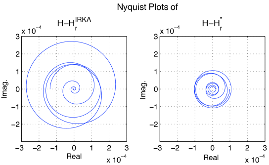
Figure 10: The error curve for $H_{r}^{\star}$ is nearly circular

4 Conclusions

We have introduced an interpolation-based model reduction technique to construct high-fidelity $\mathcal{H}_{\infty}$ approximations for large-scale linear dynamical systems. For a given order $r$, $r$ Hermite interpolation points are produced that induce (locally) optimal $\mathcal{H}_{2}$ approximation. The $d_{r}$ (feed-forward) term is then adjusted in a such way that interpolation at these initial $2r$ points is retained while an additional interpolation point is added that minimizes the $\mathcal{H}_{\infty}$-error norm. By employing a data-driven Loewner approach, this last step may be performed at negligible cost; no large-scale $\mathcal{H}_{\infty}$-norm computations are ever needed. The dominant cost of the method lies with the solution of sparse linear systems. Four numerical examples show that the proposed method produces high fidelity $\mathcal{H}_{\infty}$ reduced-order models that are better than those obtained by balanced truncation; and as good as (and sometimes better than) those obtained by optimal Hankel norm approximation; in all cases, at much lower computational cost.

References

- Antoulas [2005] A.C. Antoulas. Approximation of Large-Scale Dynamical Systems (Advances in Design and Control). Society for Industrial and Applied Mathematics, Philadelphia, PA, USA, 2005.
- Antoulas and Astolfi [2004] A.C. Antoulas and A. Astolfi. -norm approximation. In V.D. Blondel and A. Megretski, editors, Unsolved Problems in Mathematical Systems and Control Theory, pages 267–270. Princeton University Press, USA, 2004.
- Antoulas et al. [2001] A.C. Antoulas, D.C. Sorensen, and S. Gugercin. A survey of model reduction methods for large-scale systems. Contemporary Mathematics, 280:193–219, 2001.
- Antoulas et al. [2010] A.C. Antoulas, C.A. Beattie, and S. Gugercin. Interpolatory model reduction of large-scale dynamical systems. In J. Mohammadpour and K. Grigoriadis, editors, Efficient Modeling and Control of Large-Scale Systems. Springer-Verlag, 2010.
- Beattie and Gugercin [2009a] C. Beattie and S. Gugercin. Interpolatory projection methods for structure-preserving model reduction. Systems & Control Letters, 58(3):225 – 232, 2009a.
- Beattie and Gugercin [2007] C.A. Beattie and S. Gugercin. Krylov-based minimization for optimal model reduction. 46th IEEE Conference on Decision and Control, pages 4385–4390, Dec. 2007.
- Beattie and Gugercin [2009b] C.A. Beattie and S. Gugercin. A trust region method for optimal model reduction. 48th IEEE Conference on Decision and Control, Dec. 2009b.
- Benner [2004] P. Benner. Solving large-scale control problems. Control Systems Magazine, IEEE, 24(1):44–59, 2004.
- Benner and Saak [2004] P. Benner and J. Saak. Efficient numerical solution of the LQR-problem for the heat equation. Proc. Appl. Math. Mech, 4(1):648–649, 2004.
- Benner et al. [2003] P. Benner, E. S. Quintana-Ortí, and G. Quintana-Ortí. State-Space Truncation Methods for Parallel Model Reduction of Large-Scale Systems. Parallel Computing, special issue on “Parallel and Distributed Scientific and Engineering Computing”, 29:1701–1722, 2003.
- Benner et al. [2004] P. Benner, E.S. Quintana-Orti, and G. Quintana-Orti. Computing optimal Hankel norm approximations of large-scale systems. In Proceedings of 43rd IEEE Conference on Decision and Control, volume 3, pages 3078 – 3083, December 2004.
- Chahlaoui and Van Dooren [2005] Y. Chahlaoui and P. Van Dooren. Benchmark examples for model reduction of linear time-invariant dynamical systems. Dimension Reduction of Large-Scale Systems, 45:381–395, 2005.
- Flagg [2009] G.M. Flagg. An interpolation-based approach to optimal model reduction. Master’s thesis, Virginia Tech, Department of Mathematics, May 2009.
- Glover [1984] K. Glover. All optimal Hankel-norm approximations of linear multivariable systems and their -error bounds. Int J Control, 39(6):1115–1193, 1984.
- Grigoriadis [1995] K.M. Grigoriadis. Optimal model reduction via linear matrix inequalities: continuous- and discrete-time cases. Systems & Control Letters, 26(5):321 – 333, 1995.
- Grimme [1997] E.J. Grimme. Krylov projection methods for model reduction. PhD thesis, University of Illinois, 1997.
- Gugercin [2005] S. Gugercin. An iterative rational Krylov algorithm (IRKA) for optimal model reduction. In Householder Symposium XVI, Seven Springs Mountain Resort, PA, USA, May 2005.
- Gugercin [2002] S. Gugercin. Projection methods for model reduction of large-scale dynamical systems. PhD thesis, Ph. D. Dissertation, ECE Dept., Rice University, 2002.
- Gugercin and Antoulas [2004] S. Gugercin and A.C. Antoulas. A survey of model reduction by balanced truncation and some new results. International Journal of Control, 77(8):748–766, 2004.
- Gugercin et al. [2003] S. Gugercin, D.C. Sorensen, and A.C. Antoulas. A modified low-rank Smith method for large-scale Lyapunov equations. Numerical Algorithms, 32(1):27–55, 2003.
- Gugercin et al. [2008] S. Gugercin, A.C. Antoulas, and C. Beattie. model reduction for large-scale linear dynamical systems. SIAM Journal on Matrix Analysis and Applications, 30(2):609–638, 2008.
- Heinkenschloss et al. [2008] M. Heinkenschloss, D.C. Sorensen, and K. Sun. Balanced Truncation Model Reduction for a Class of Descriptor Systems with Application to the Oseen Equations. SIAM Journal on Scientific Computing, 30:1038, 2008.
- Helmersson [1994] A. Helmersson. Model reduction using LMIs. In Proceedings of the 33rd IEEE Conference on Decision and Control, volume 4, pages 3217–3222, December 1994.
- Kavranoglu [1995] D. Kavranoglu. approximation of discrete-time systems by constant matrices. Numerical Functional Analysis and Optimization, 16:177–196, 1995.
- Kavranoglu [1993] D. Kavranoglu. Zeroth order norm approximation of multivariable systems. Numerical Functional Analysis and Optimization, 14(1):89–101, 1993.