SPIDER - V. Measuring Systematic Effects in Early-Type Galaxy Stellar Masses from Photometric SED Fitting

Abstract

We present robust statistical estimates of the accuracy of early-type galaxy stellar masses derived from spectral energy distribution (SED) fitting as functions of various empirical and theoretical assumptions. Using large samples consisting of 40,000 galaxies from the Sloan Digital Sky Survey, of which 5,000 are also in the UKIRT Infrared Deep Sky Survey, with spectroscopic redshifts in the range 0.05 $\leq$ z $\leq$ 0.095, we test the reliability of some commonly used stellar population models and extinction laws for computing stellar masses. Spectroscopic ages (t), metallicities (Z), and extinctions (A) are also computed from fits to SDSS spectra using various population models. These constraints are used in additional tests to estimate the systematic errors in the stellar masses derived from SED fitting, where t, Z, and A are typically left as free parameters. We find reasonable agreement in mass estimates among stellar population models, with variation of the IMF and extinction law yielding systematic biases on the mass of nearly a factor of 2, in agreement with other studies. Removing the near-infrared bands changes the statistical bias in mass by only 0.06 dex, adding uncertainties of 0.1 dex at the 95% CL. In contrast, we find that removing an ultraviolet band is more critical, introducing 2? uncertainties of 0.15 dex. Finally, we find that stellar masses are less affected by absence of metallicity and/or dust extinction knowledge. However, there is a definite systematic offset in the mass estimate when the stellar population age is unknown, up to a factor of 2.5 for very old (12 Gyr) stellar populations. We present the stellar masses for our sample, corrected for the measured systematic biases due to photometrically determined ages, finding that age errors produce lower stellar masses by 0.15 dex, with errors of 0.02 dex at the 95% CL for the median stellar age subsample.

1 Introduction

Our understanding of the formation and evolution of early-type galaxies (ETGs) represents a key ingredient in models of galaxy formation. Here, we consider ETGs to be bulge dominated galaxies with passive spectra in their central regions. Observationally, they are characterized by elliptical isophotes, generally redder colors, and a sharp 4000Å break, corresponding to an accumulation of absorption lines of mainly ionized metals, reflected in their rest frame UV/optical colors. This feature is typical of old stellar populations with little to no ongoing star formation.

At higher redshift, most ETGs can only be studied in integrated light, and interpretation of their photometric and spectroscopic properties requires population synthesis models. These single stellar population (SSP) models usually consist of stars born at the same time with equal initial element compositions, evolved using the isochrone synthesis technique (see Charlot & Bruzual, 1991 for a review), where stars of different masses follow different evolutionary tracks. SSP models can be combined to produce arbitrary star-formation histories, although most studies restrict themselves to histories with exponentially declining star-formation. Such tau-models are parametrized by the e-folding time of this decline, $\tau$. The spectral energy distributions (SEDs) from a set of models with various parameters (e.g. initial mass function (IMF), star-formation history, age, metallicity, and extinction) is compared to the photometric or spectroscopic observations to derive a best-fit template. A fundamental parameter derived from such SED fitting is the overall normalization of the model relative to the observations, which gives the galaxy stellar mass content. Indeed, a measurement of the stellar mass of an ETG is involved in many useful scaling relations, such as the size-mass relation (Shen et al., 2003) and downsizing (Cowie et al., 1996), where the evolutionary history of ETGs is seen to follow different time scales as a function of their stellar mass content. Stellar mass assembly in galaxies is also used in tests of hierarchical models, such as the evolution of the number density and size of both early and late-type galaxies as a function of redshift (Bell et al., 2003; Bundy et al., 2005; Ilbert et al., 2010). Furthermore, upcoming surveys (e.g. PanSTARRS, LSST, DES) will provide only photometry, so it is crucial to understand how to obtain reliable stellar masses from SED fitting techniques.

The degeneracies among the multiple model parameters which are required to reproduce the observed SEDs of the galaxies, along with the available photometric bandpasses, determine the uncertainty of the mass estimates. For example, models and observations show that the rest-frame near-infrared (NIR) galaxy flux correlates well with stellar mass (Kauffmann & Charlot, 1998; Cowie et al., 1996) due to weak contributions from hot, young stars and dust extinction at these wavelengths. But both different model predictions and/or absence of NIR data in fitting the SED can result in stellar masses which differ by a factor of 2, for both low and high redshift samples (van der Wel et al., 2006). Of particular interest in this study, the effects of unknown stellar population age, metallicity, and extinction on the stellar masses derived for elliptical galaxies have not been quantified. It is already well known that the age-metallicity degeneracy (Worthey, 1994) cannot easily be broken with broadband colors alone.

All of these factors either depend on or affect the resulting evolution of the spectral energy distribution, models of which have been generated by, e.g. Bruzual & Charlot (2003), Maraston (2005), and Fioc & Rocca-Volmerange (1997). Many phases in stellar evolution are still not well understood, but one key ingredient in these models, the thermally-pulsating asymptotic giant branch (TP-AGB) phase, is particularly influential for determining the galaxy stellar mass for a range of dominant stellar population ages. Light from these stars largely influences the integrated brightness of the NIR continuum, the effects of which were recently highlighted by Maraston et al. (2006) and Bruzual (2007), who found systematic differences of factors of $\sim$2 in mass and age over a large range in redshift. This example has shown us the effects of one sensitive parameter in the SED fitting process and demonstrates the need to further test the dependence of the stellar mass estimate on model parameters and the use of common ground-based observation filters.

Several authors (e.g. Conroy et al., 2009; Treu et al., 2010; Raichoor et al., 2011) have studied some of these effects on the photometrically derived stellar mass, quantifying systematic offsets between masses calculated against different model parameters. However, they all suffer from a lack of spectroscopic data which can provide independent constraints on many of the galaxy properties. Longhetti & Saracco (2009) used a synthetic catalog of intermediate redshift ($1\leq z\leq 2$) ETGs to test the dependence of stellar population models and assumed model parameters on stellar mass. However, they compare a synthetic catalog to only 125 galaxies observed in the GOODS field, using a different SED fitting code. Ilbert et al. (2010) and Bernardi et al. (2010) test the accuracy of large surveys ($\sim$10,000 and $\sim$200,000 galaxies, respectively) at estimating photometric stellar masses compared to those from available spectroscopy. However, these projects select mostly galaxies at high redshift and neglect the possible combined effects of assuming various free parameters.

This paper is part of a series examining the global and internal properties of ETGs in the nearby Universe, combining optical and NIR photometry with spectroscopic data. The Spheroids Panchromatic Investigation in Different Environmental Regions (SPIDER) project is described in La Barbera et al. (2010a, hereafter Paper I). The second and third papers of the series present a thorough analysis of the optical+NIR scaling relations of ETGs (La Barbera et al., 2010b, c), while in Paper IV (La Barbera et al., 2010d) we have analyzed the optical+NIR internal color gradients of ETGs. Here we present an extensive comparison of stellar mass estimates obtained for low redshift ETGs by varying several observational and model parameters (presented individually in Section 7). The paper is organized as follows. Section 2 describes the galaxies, comprised of a carefully selected sample of high S/N, low redshift ETGs. In Section 3 we describe the different stellar population models used to compute model galaxy SEDs. In Section 4 we provide an overview of the general technique applied to fit the theoretical SEDs to the observed colors and the SDSS galaxy spectra. The reliability of these fits is assessed in Section 5, by comparing photometric and spectroscopic fitting results. Our method for determining stellar masses is described in Section 6, while the results of the various model comparisons are discussed in Section 7. Throughout the paper, we adopt a cosmology with H${}_{0}=70$ km s^-1 Mpc^-1, $\Omega_{m}=0.3$, and $\Omega_{\Lambda}=0.7$.

2 The SPIDER sample

2.1 SDSS $ugriz$ sample of ETGs

The sample of galaxies is selected from the Sloan Digital Sky Survey (SDSS) DR6 in the redshift range 0.05 to 0.095 and with $M_{r}<-20$, where $M_{r}$ is the k-corrected SDSS Petrosian magnitude in the r-band. The k-correction is estimated using the software kcorrect (Blanton et al., 2003), through a rest frame r-band filter blue-shifted by a factor $(1+z_{0})$, where $z_{0}=0.0725$, the median redshift of the ETG sample (see Paper I, Section 3.1). The lower redshift limit is chosen to minimize the aperture bias (Gómez et al., 2003), while the upper redshift limit guarantees a high level of completeness (according to Sorrentino et al., 2006) and allows us to define a volume-complete sample of bright early-type systems. ETGs follow two different trends in the size-luminosity diagram (Capaccioli et al., 1992; Graham & Guzmán, 2003). The separation between these two families of bright and ordinary ellipticals occurs at an absolute B-band magnitude of $-$19, corresponding to the magnitude limit of $M_{r}\sim-20$ adopted for this selection. At the upper redshift limit of $z=0.095$, the magnitude cut of $-20$ also corresponds approximately to the magnitude limit where the SDSS spectroscopy is complete (i.e. Petrosian magnitude of $m_{r}\sim 17.8$), making the sample volume limited. Following Bernardi et al. (2003), we define ETGs using the SDSS spectroscopic parameter eClass, which indicates the spectral type of a galaxy on the basis of a principal component analysis, and the SDSS photometric parameter fracDev_r, which measures the fraction of galaxy light that is better fitted by a de Vaucouleurs (rather than an exponential) law. In this contribution, ETGs are those systems with $eClass<0$ and $fracDev_{r}>0.8$. The SDSS selection criteria and completeness of the ETG sample, part of the SPIDER project, are further detailed in Paper I.

2.2 UKIDSS $YJHK$ photometry

The SPIDER sample consists of 39,993 ETGs, with available ugriz photometry and spectroscopy. This SDSS sample is then matched to the UKIRT Infrared Deep Sky Survey (UKIDSS) Large Area Survey DR4. The UKIDSS-LAS DR4 provides NIR photometry in the $YJHK$-bands over $\sim$1000 square degrees on the sky, with significant overlap with SDSS. The $YHK$-band data have a pixel scale of $0.4^{\prime\prime}$ pixel^-1, matching almost exactly the resolution of the SDSS frames ($0.396^{\prime\prime}$ pixel^-1). $J$-band observations are carried out with a resolution of $0.4^{\prime\prime}$ pixel^-1, and then interleaved to a subpixel grid, resulting in stacked frames with a resolution of $0.2^{\prime\prime}$ pixel^-1. The $YJHK$-stacked images (multiframes) have average depths of 20.2, 19.6, 18.8, and 18.2 magnitudes (in the Vega system), respectively. For each ETG in the SDSS sample, we searched for the nearest UKIDSS detection within a radius of $1^{\prime\prime}$, considering only UKIDSS frames with good quality flags ($ppErrBits<16$). Of these galaxies, 5,080 objects also have available photometry in the YJHK wavebands from UKIDSS. Hereafter, we refer to these samples as the complete and optical+NIR samples of ETGs, respectively.

As detailed in Paper I, all grizYJHK frames have been homogeneously processed with 2DPHOT (La Barbera et al., 2008), an automated software environment that performs several tasks, such as catalog extraction (using SExtractor), star/galaxy separation, and galaxy surface photometry. For each ETG, magnitudes are measured within the same aperture in all $ugrizYJHK$ wavebands. Unless otherwise stated, in the present work we use the $ugrizYJHK$ magnitudes measured within an adaptive circular aperture of $3\times r_{K,i}$, where $r_{K,i}$ is the Kron radius in the $i$-band. We use $i$-band Kron radii because of the larger S/N ratio of $i$ relative to $zYJHK$ frames (see Section 5), and its lower sensitivity to young stellar populations in a galaxy relative to $ugr$. All magnitudes herein are in the AB system. For more than 95% of all ETGs in the SPIDER sample, the $3\times r_{K,i}$ aperture is at least three times larger than the seeing FWHM of the $grizYJHK$ frames, making the Kron magnitudes essentially independent of the seeing variation from $g$ through $K$ (see Paper I). We also note that the first four papers in this series do not use $u$-band photometry, as the S/N of SDSS $u$-band frames is too low to measure reliable surface photometry. For the present study, we have processed the $u$-band images with SExtractor (Bertin & Arnouts, 1996), using the same setup as for the $grizYJHK$ wavebands, now resulting in 5,068 objects in the optical+NIR sample. All magnitudes have been corrected for Galactic extinction, as detailed in Paper I.

2.3 SDSS spectroscopy

SDSS spectra in the range $3800-9200$Å are analyzed with the spectral fitting code STARLIGHT (Cid Fernandes et al., 2005) to determine galaxy ages, metallicities, and interstellar extinctions, among other parameters. STARLIGHT finds the combination of SSP models that, normalized and broadened with a given sigma, best matches the observed spectrum. To this effect, objects are de-redshifted and corrected for foreground extinction, following the recipes described in Paper I. For the galaxy spectra in the SPIDER sample, the median value of the resolution varies from $\sim$2.8Å (FWHM) in the blue (4000Å) up to $\sim$3.7Å (FWHM) in the red (8000Å). The theoretical spectra used for comparison (and described below in Section 3) have similar resolution to that of SDSS spectra across the whole wavelength range from $\sim$3000Å to $\sim$9000Å and are therefore not resampled for this study.

3 Stellar population models

We begin by constructing a library of model spectra (SEDs), generated through different stellar population synthesis techniques that encompass a variety of stellar evolutionary tracks. The models span a wide range in age, metallicity, extinction, and IMF. In the following, we describe the SEDs used to fit the broadband colors as well as the spectra of ETGs.

3.1 SEDs for fitting broadband colors

We use stellar population synthesis models to convert galaxy luminosity into stellar mass (e.g. Bell et al., 2003; Fontana et al., 2004). The stellar mass is derived from the factor needed to rescale the spectrum from the best fit theoretical stellar population (normalized at 1 $\mathcal{M}_{\sun}$) to the intrinsic (observed) luminosities. The models we use to fit galaxy colors are described below.

3.1.1 Bruzual & Charlot (2003)

Among the variety of stellar evolution libraries provided by this code (hereafter BC03), we use models from the Padova 1994 library, which provide a median spectral resolution $R=2000$ over the spectral range from 3200 to 9500Å (STELIB), and $R=300$ outside this range (BaSeL 3.1; see BC03 for details). Models of stars with $T>50,000$ K are taken from Rauch (2003), and the spectral models of the thermally-pulsating asymptotic giant branch (TP-AGB) phase are based on Vassiliadis & Wood (1993). We utilize models with four different metallicities: $0.2Z_{\sun},0.4Z_{\sun},Z_{\sun},\mathrm{and}~{}2.5Z_{\sun}$. Within this code, we also consider both Salpeter (1955) and Chabrier (2003) IMFs, with mass limits of $0.1M_{\sun}<M<100M_{\sun}$. Unless otherwise noted, we assume a Chabrier IMF due to its theoretical motivation. The star-formation histories include exponentially declining $SFR\propto e^{-t/\tau}$ with the values of $\tau$ given below, no gas recycling, and a $t=20$ Gyr cutoff time for star-formation. This ensures that no models have their SF cut off before an e-folding time. Table 1 provides a summary of the stellar population model parameters, where the last column provides stellar ages used in comparing LePhare and STARLIGHT results (discussed in Section 5).

Table 1: Stellar population model parameters (BC03/CB10).

$\tau$			$t_{SSP}$
(Gyr)	$E(B-V)$	$Z/Z_{\sun}$	(Gyr)
0.1	0	0.2	0.5, 1.0, 2.0,
0.3	0.1	0.4	2.2, 2.5, 2.75,
1	0.2	1.0	3.25, 3.5, 4.0,
2	0.3	2.5	4.5, 5.0, 5.5,
3	0.4		6.25, 7.0, 8.0,
5	0.5		9.0, 10.0, 11.25
10			12.5
15
30

The SEDs were generated for a grid of 64 ages in the range 0.8$-$14.2 Gyr. Since the mixing of dust and stars in (early-type) galaxies is far from well understood, for the purposes of the present work we describe dust extinction with a simplified approach, where attenuation is applied to the templates using the Cardelli et al. (1989) law, with $E(B-V)$ in the range 0$-$0.5. The reddening $E(B-V)$ is limited to 0.5 magnitudes to avoid incorrect fitting of observationally red galaxies as highly reddened blue galaxies; such objects should be absent from our sample. Ilbert et al. (2010) show that the stellar mass measurements are sensitive to the extinction law, with absolute median differences of 0.14 and 0.27 dex for two spectroscopic samples of high redshift galaxies when comparing the Calzetti et al. (2000) and Charlot & Fall (2000, CF2000) extinction laws. We present similar results in Section 7.7. Unless otherwise noted, we use the Cardelli extinction law throughout this paper. We note that most studies using SED fitting to determine stellar masses have used the Calzetti extinction law. However, this law is theoretically motivated for strong starbursts. While this may be reasonable for field surveys, where the majority of galaxies are likely to be star-forming, it is inappropriate for our sample, where we expect ETGs to be dominated by older stellar populations. Therefore, we utilize the Cardelli relation as our baseline.

3.1.2 Charlot & Bruzual (2010)

An updated version of this code, which includes the new prescription of Marigo & Girardi (2007) for the TP-AGB evolution of low and intermediate-mass stars, is described in Bruzual (2007) and is used in previous papers in this series (Papers II, III, IV). We consider its preliminary version in the following comparisons, referring to it as the CB10 code (Charlot & Bruzual, private communication). These templates use the STELIB library over the entire wavelength range covered by the $ugrizYJHK$ bands. We use the same stellar population parameters as BC03, described above and listed in Table 1.

3.1.3 PEGASE.2: Fioc & Rocca-Volmerange (1997)

The code by Fioc & Rocca-Volmerange (1997) is based on the same tracks and the same stellar spectral library as BC03. The difference between the spectrophotometric models is given by different stellar spectra assumptions for the hottest stars ($T>50,000K$) and a different prescription for the TP-AGB phase, both affecting the results at young ages ($\leq 2$ Gyr). Indeed, spectra of hot stars are taken from Clegg & Middlemass (1987), while the models of the TP-AGB phase are based on the prescriptions of Groenewegen & de Jong (1993). For comparison with the results obtained with the BC03/CB10 codes, we have used models with exponentially declining SFR with time scales $\tau=0.1,0.3,1.0,2.0,3.0,5.0,10.0,\mathrm{and}~{}15.0$ Gyr and a Scalo (1986) IMF. Solar metallicity is assumed for each template, based on the readily available models within LePhare. The models are set up with no infall (i.e. all the gas available to form stars is assumed to be in place at time $t=0$) and no galactic wind, and the default value of 0.05 has been assumed for the parameter representing the fraction of close binary systems. Because this library is available in the public version of LePhare, we choose to compare its results here.

The SEDs were generated for a grid of 39 ages (in the range 0.8$-$14.2 Gyr). Dust extinction was applied to the templates, using the Cardelli et al. (1989) law (again with $E(B-V)$ in the range 0$-$0.5).

3.2 SEDs for fitting spectra

For each galaxy in the optical+NIR sample, we fit BC03/CB10 templates in the wavelength range 3800$-$9200Å to its SDSS spectrum. Per other studies using this sample, we also run STARLIGHT using SSPs from (Vazdekis et al., 2010, hereafter, M09) that are based on the MILES stellar library (Sánchez-Blázquez et al., 2006), which has an almost complete coverage of stellar atmospheric parameters, containing spectra of stars in the solar neighborhood. These SEDs cover the spectral range 3800$-$7500Å with a spectral resolution of 2.3Å. Hence, they are well suited to analyzing SDSS spectra, whose spectral resolution is $\sim$2.36Å (FWHM) in the wavelength interval 4800$-$5350Å. By improving on the instrumental homogeneity among stellar spectra, which share the same wavelength scale and resolution, and the accuracy of relative flux calibrations as compared to previous stellar population model catalogs, we expect M09 to contribute only small systematic biases in the estimates of spectroscopic parameters. Since support for the M09 library is not provided within LePhare by default, and given the minimal usable wavelength range, we have opted to use BC03 models in the photometric SED fitting to compute the theoretical magnitudes, provided reliable spectroscopic measurements are obtained from the M09 models.

To run STARLIGHT, we select a basis of 76 MILES SSPs, with ages and metallicities listed in Table 1. All models have [$\alpha/Fe$]$=0$ (i.e. solar abundance ratio). Dust extinction was applied to the templates, using the Cardelli et al. (1989) law.

4 SED fitting using a $\chi^{2}$-minimization

The theoretical SEDs are compared with either the observed galaxy colors or the observed spectra to determine the age, metallicity, and color excess $E(B-V)$ that best fits the observations. In the case of galaxy colors, the stellar population models (see Section 3) can be used to produce theoretical SEDs at different redshifts, and hence the fitting provides an estimate of the photometric redshift (see Benítez (2000) for a review).

4.1 Fitting broadband photometry with LePhare

We perform the SED fitting with the photometric redshift code LePhare (Arnouts et al., 1999; Ilbert et al., 2006), which uses a $\chi^{2}$-minimization technique. Other popular photometric redshift codes have been tested on various figures of merit. Abdalla et al. (2008) use $\sim$13,000 spectroscopic redshifts from luminous red galaxies in SDSS DR6 to test six publicly available photometric redshift codes, including LePhare and the popular codes HyperZ (Bolzonella et al., 2000) and BPZ (Benítez, 2000), finding that LePhare performs best in the lower redshift intervals. This result and the existing collaboration with the code developers motivates this choice for our study. Each SED is redshifted up to $z=0.3$ in steps of $\delta z=0.005$ and convolved with the SDSS/UKIDSS filter transmission curves . The opacity of the intergalactic medium (Madau, 1995) is taken into account within LePhare. The merit function $\chi^{2}$ is defined as

$$\chi^{2}(z,T,A)=\sum_{f=1}^{N_{f}}\left(\frac{F_{obs}^{f}-A\times F_{pred}^{f}(z,T)}{\sigma_{obs}^{f}}\right)^{2},$$ (1)

where $F_{pred}^{f}(T,z)$ is the flux predicted for a template $T$ at redshift $z$. $F_{obs}^{f}$ is the observed flux and $\sigma_{obs}^{f}$ is the associated error, converted from the AB system. The index $f$ refers to the specific filter and $N_{f}$ is the number of filters. The photometric redshift is estimated from the minimization of $\chi^{2}$ varying the three free parameters $z$, $T$, and the normalization factor $A$. This normalization factor depends on the choice of waveband used for scaling and is calculated as

$$A=\sum_{\tilde{f}=1}^{N_{\tilde{f}}}\left(\frac{F_{obs}^{\tilde{f}}\times F_{pred}^{\tilde{f}}}{(\sigma_{obs}^{\tilde{f}})^{2}}\right)/\sum_{\tilde{f}=1}^{N_{\tilde{f}}}\left(\frac{F_{pred}^{\tilde{f}}}{\sigma_{obs}^{\tilde{f}}}\right)^{2},$$ (2)

where $\tilde{f}$ refers to the waveband(s) used for scaling. Studies often use near-infrared bands (e.g. $K$-band) for scaling, since it is only weakly affected by dust extinction and is quite insensitive to the presence of young, luminous stars (Lilly & Longair, 1984; Glazebrook et al., 1995; Cowie et al., 1996). In Section 7.4, we present a comparison of galaxy stellar masses for several choices of band scaling. Here, we note only that it produces a negligible difference in the mass and, unless otherwise noted, we utilize all available wavebands to scale the SED.

4.1.1 Improving data and model matching with photometric zero-point offsets

The SDSS/UKIDSS photometric zero-points are uncertain at the few percent level (see Fukugita et al. (1996); Hewett et al. (2006), respectively). To insure further accuracy of data and model flux matching, it is important to provide reliable uncertainties in the zero-point magnitudes. To this end, we utilize the complete and optical+NIR samples with spectroscopic redshifts, including objects in the range $14.0\leq i\leq 16.4$ (brighter 25% of ugrizYJHK galaxies). Using a $\chi^{2}$-minimization (Equation 1) at fixed redshift, we determine for each galaxy the corresponding best-fitting stellar population template. LePhare notes in each case $F_{obs}^{f}$, the observed flux in the filter $f$. $A\times F_{pred}^{f}$ is the predicted flux derived from the best fit template and rescaled using the normalization factor $A$ of Equation 2. For each filter $f$, the sum

$$\psi^{2}=\sum^{N_{gal}}\left(\left(A\times F_{pred}^{f}-F_{obs}^{f}+s^{f}\right)/\sigma_{obs}^{f}\right)^{2}$$ (3)

is minimized, leaving $s^{f}$ as a free parameter. For random, normally distributed uncertainties in the flux measurement, the average deviation $s^{f}$ should be zero. Instead, we observe some systematic differences, which are listed for the optical+NIR sample at fixed redshift in Table 2 (median, converted to magnitudes. In our data, these differences never exceed $0.042$ mag (Y-band) and have an average amplitude of $0.019$ mag, using BC03. We see that these differences depend very weakly on the magnitude cut, listed as $14.0\leq m_{i}\leq x$, adopted to select the sample and are also almost independent from the set of templates used in the fitting. The sizes of these systematic differences are comparable to the level at which the SDSS/UKIDSS photometric systems differ from a true AB system. We then proceed to correct the predicted apparent magnitudes for these systematic differences, using the correction factor $s^{f}$. If we repeat a second time the procedure of template fitting after having adjusted the zero-points, the best fit templates may change. LePhare checks that the process is converging: after two iterations each estimated correction $s^{f}$ varies less than 0.0013 mag. Since the uncertainties in these zero-point corrections are not less than 0.01 mag, this error is added in quadrature to the apparent magnitude errors.

Table 2: Systematic differences $s^{f}$ between the observed and predicted fluxes.

filter	BC03	BC03	BC03	CB10	PEGASE.2
	$i\leq$ 16.4	$i\leq$ 16.8	$i\leq$ 17.1	$i\leq$ 16.4	$i\leq$ 16.4
$u$	-0.021	-0.026	-0.026	-0.020	-0.161
$g$	0.011	0.010	0.009	0.012	0.003
$r$	-0.006	-0.004	-0.004	-0.004	0.050
$i$	-0.013	-0.012	-0.011	-0.035	-0.013
$z$	0.004	0.005	0.005	-0.017	0.019
$Y$	0.042	0.042	0.041	0.062	0.093
$J$	-0.029	-0.027	-0.025	-0.012	-0.034
$H$	-0.021	-0.023	-0.025	-0.025	-0.049
$K$	0.027	0.026	0.026	0.015	-0.064

4.2 Spectral fitting

For each spectrum in the optical+NIR sample, we run STARLIGHT (Cid Fernandes et al., 2005) using a suite of models with stellar population parameters given in Table 1, separately for BC03/CB10 and M09 (see Section 3.2). The code uses a $\chi^{2}$-minimization, with a figure of merit given by

$$\chi^{2}(\textbf{\emph{x}},A_{V},v_{*},\sigma_{*})=\sum_{\lambda}\left[\left(\mathcal{O}_{\lambda}-\mathcal{T}_{\lambda}\right)\omega_{\lambda}\right]^{2},$$ (4)

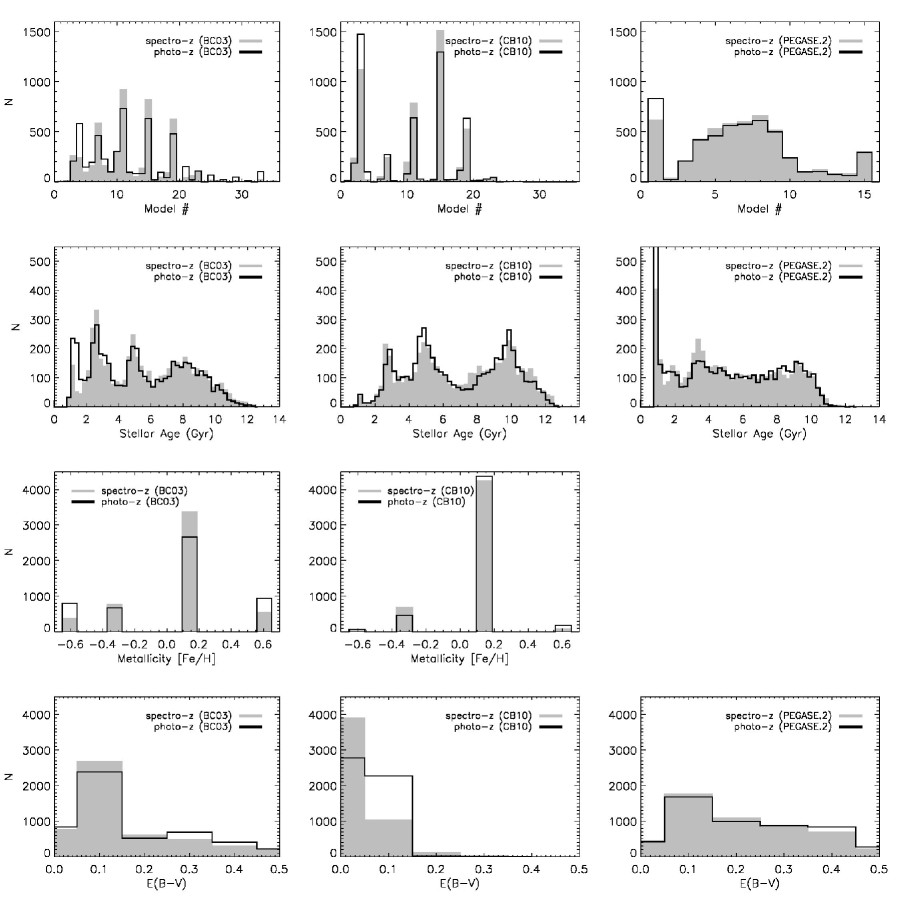
Figure 1: Distributions of models, ages, metallicities, and color excesses, using BC03 ($left$), CB10 ($center$), and PEGASE.2 ($right$). See Table 6 for “Stellar Population Model #” information. $Gray$ histograms use the spectro-z, and $black$ histograms use the photo-z. Note that PEGASE.2 templates use solar metallicity. Stellar age is measured using the median of $\exp(-\chi^{2}/2)$ from all fits, whereas LePhare only provides model (metallicity) and $E(B-V)$ from the best $\chi^{2}$ value.

where $\mathcal{O}_{\lambda}$ is the observed spectrum at wavelength $\lambda$, $\mathcal{T}_{\lambda}$ is the model spectrum, and $\omega_{\lambda}$ is a weighting factor. The model spectrum is a convolution of the intrinsic spectrum x with a Gaussian filter centered at $v_{*}$ with dispersion $\sigma_{*}$. Since both BC03/CB10 and M09 have similar spectral resolutions to the SDSS spectra, the $\sigma_{*}$ provides a direct estimate of the galaxy velocity dispersion (see Paper I for details). The intrinsic spectrum x is a linear combination of a set of stellar population models (the base) provided as input to the code. The coefficients of this linear combination are computed from STARLIGHT as part of the $\chi^{2}$-minimization procedure. For our purposes, we do not use this feature of STARLIGHT, but rather use the reduced-$\chi^{2}$ statistic provided by the code for each model in the base to compute the age, [Fe/H], and $A_{V}$ of the best fit (i.e. lowest $\chi^{2}$) stellar population model. For processing efficiency the code permits a maximum of 300 base models, so to allow a reasonably dense grid of ages/metallicities (columns 3,4 of Table 1), we chose to use single ($t=0$) burst models, which is justified by the mostly short-burst fits shown in Figure 1 (see top panels). Here we plot the distribution of best fit BC03/CB10/PEGASE.2 models for the optical+NIR sample, where the abscissa shows increasing $\tau$ (i.e. decay time scale for star-formation), with every fourth value being a constant metallicity – for reference, the first five peaks (BC03/CB10) represent solar metallicity models with $\tau\leq 3$ Gyr. A comparison of best fit ages, metallicities, and extinctions between LePhare and STARLIGHT is given in Section 5.2.

5 SED fitting reliability

In this section, we compare results obtained by fitting broadband colors and spectra of ETGs. We begin by comparing photometric and spectroscopic redshifts in Section 5.1, while in Section 5.2 we compare age, metallicity, and internal extinction estimates between LePhare and STARLIGHT.

5.1 Accuracy of photometric redshifts

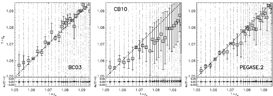
Figure 2: Comparison between the spectroscopic and photometric redshifts, having corrected for zero-point magnitude offsets (see Section 4.1.1) with a bright subsample $14.0\leq m_{i}\leq 16.4$. $Top$ panels show redshifts for the optical+NIR sample, with $squares$ representing the median values in each bin (200 objects) and their 2$\sigma$ uncertainties. $Bottom$ panels show residuals, $z_{s}-z_{p}$, normalized by the spectro-z.

We compare spectroscopic and photometric redshifts for the optical+NIR sample in Figure 2. The galaxies are binned to include 200 objects per $\delta z_{spec}$ bin, and the error bars denote the dispersion defined by $1.48\times\mathrm{median}(|\Delta z|/(1+z_{spec}))$. This measurement of the scatter corresponds to the rms for a Gaussian distribution and is unaffected by outliers (Ilbert et al., 2006). We recover $\sim$73% of the galaxies (BC03) with outlier rate, defined here as $\eta=|\Delta z|<0.025(1+z_{spec})$. The accuracy of these photometric redshifts improved with addition of the u-band data by $\sim$7% in the outlier rate. Ilbert et al. (2006) use their sample of $\sim$3,000 galaxies to confirm the importance of the u-band for low redshift galaxies, recovering $\sim$80% of the photometric redshifts at $z<0.4$ and $\sim$95% using the u-band. Figure 2 shows the binned redshifts, using the Chabrier (Scalo) IMF for BC03/CB10 (PEGASE.2) stellar population models, and the Cardelli extinction law. Photometric redshifts are well recovered, given the small redshift range, with outlier rates of $\sim$73%, $\sim$75%, $\sim$76% for BC03/CB10/PEGASE.2, respectively. However, at higher redshifts, CB10 models produce systematically lower photometric redshifts. This is surprising given the improvements described in Bruzual (2007), although it does not change the results that follow, which use the spectroscopic redshift. We note that the extremely small redshift range of our sample makes these photo-z tests unsuitable for drawing conclusions for typical imaging surveys.

5.2 Comparing photometric & spectroscopic measurements

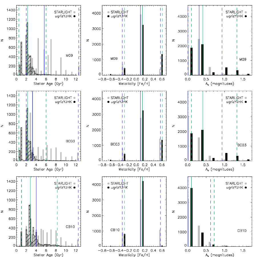
Figure 3: Comparison between spectroscopic ($gray$) and photometric ($black$) ages, metallicities, and extinctions for the optical+NIR sample. Stellar population models assume single bursts at $t=0$ and the parameters in Table 1. STARLIGHT measured extinction has been binned to the six $E(B-V)$ values in the range $0-0.5$ (converted to extinction in magnitudes using $R_{V}=3.1$. $Solid$ $blue$ ($green$) lines show the sample median, measured with STARLIGHT (LePhare), with their 2$\sigma$ uncertainties shown as $dashed$ lines.

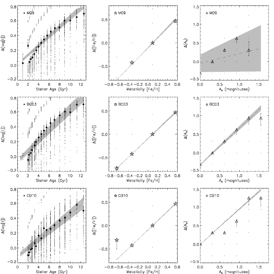
Figure 4: Each plot shows differences ($STARLIGHT-LePhare$) in spectroscopic and photometric parameters $t$, $Z$, and $A_{V}$, as a function of their spectroscopic values, measured with STARLIGHT. $Black$ symbols represent median values in each bin. Linear fits ($dashed$ lines) to the data are presented, with their 1-sigma uncertainties in the $gray$ shaded region.

To compare photometrically and spectroscopically determined results, we use the same model parameters between LePhare and STARLIGHT as much as possible. All theoretical parameters are consistent between the two packages, except for the interstellar extinction, which is calculated on-the-fly within STARLIGHT. The comparison assumes that there is essentially no stellar population gradient between the spectroscopic (fiber) and photometric (Kron) apertures. This assumption is motivated by the lack of color gradients between fiber and Kron apertures, as shown in Appendix A. As shown in Figure 3, there is good agreement between the distributions of photometric and spectroscopic ages using CB10 (see bottom-left panel), with a median difference of 0.75 Gyr, whereas the sample median age (measured from AGE_MED in LePhare) estimated from the BC03 templates is 1 Gyr too low, slightly improved by addition of the u-band data. However, the new treatment of the TP-AGB phase yields isochrones up to 1 magnitude brighter in the K-band (Bruzual, 2007), where the dominant flux of these galaxies is expected – this would produce better fits between the photometric SED and older stellar populations. Despite this discrepancy, $ugrizYJHK$ photometry reproduces the age-metallicity distribution much more accurately than the $ugriz$-bands alone, as expected, and so is used in the tests that follow. Both STARLIGHT and LePhare produce similar age/metallicity/extinction distributions for our optical+NIR sample, despite large differences for individual galaxies and strong systematic trends as a function of STARLIGHT output parameters (see Figure 4).

6 Method to estimate galaxy stellar masses

In most cases, all 9 bands were used to compute the stellar mass. We provide the rescaled template stellar mass (measured from MASS_MED in LePhare) derived from

$$\log\mathcal{M}=\log(\mathcal{M}_{*}/\mathcal{L}_{\lambda})+0.4kcor_{\lambda}+2\log d_{pc}-2.0+0.4M_{\lambda}^{sun}-0.4m_{\lambda^{\prime}},$$ (5)

where $\mathcal{M}_{*}/\mathcal{L}$ is the stellar mass-to-light ratio in the chosen filter centered at $\lambda$, $kcor_{\lambda}$ is the k-correction, $d_{pc}$ is the cosmology dependent luminosity distance in pc, and $m_{\lambda^{\prime}}$ is the apparent magnitude in the observed filter centered at $\lambda^{\prime}$ (see Longhetti & Saracco (2009) for a derivation of Equation 5). As with stellar age, this measurement is taken from the median of the likelihood function $\exp(-\chi^{2}/2)$. Note that stellar masses computed in this manner are only partial due to the adaptive aperture of $3\times r_{K,i}$; total stellar masses would require an aperture correction, which is irrelevant for this type of study (however, see Section 8). We then compute the median and its asymmetric 2$\sigma$ uncertainties for histograms of $\Delta(\log\mathcal{M})$ for differences resulting from the choices of stellar population model, initial mass function, interstellar extinction law, and photometric bands.

We also determine stellar mass, using the optical+NIR sample, for fixed age, metallicity, and extinction, derived from STARLIGHT, in Sections 7.7-7.8. We define the difference $\Delta$ as $\log\mathcal{M}_{fixed}-\log\mathcal{M}_{free}$ for each parameter. Operationally, $fixed$ refers to constraining the specified parameter and leaving all other parameters (except for redshift) free in the $\chi^{2}$-fitting. This allows us to quantify the accuracy of a stellar mass estimate when these parameters are unknown, and then derive corrections for any offset. Therefore, we define a mass correction term, $\epsilon$, which can be applied to the stellar mass measurements over a range of photometrically determined ages and metallicities, for a given best fit template (i.e. through a linear regression line). This term is computed as the median of each $\Delta(\log\mathcal{M})$ histogram described above for fixed-parameter minus free-parameter. In Section 7.8.2, we discuss the use of this parameter in correcting the stellar mass distribution of our samples.

Lastly, we present two comparisons of our measured stellar masses to similar estimates from a group at the Max Planck Institute and to those presented in Paper IV – this is discussed in Section 8. We note here that the overall agreement with separate photometrically estimated stellar masses (MPI) is excellent, showing a negligible offset with 2$\sigma$ scatter of about 0.1 dex. We find that inclusion of short-burst model SEDs when fit with a young ($\lesssim$3 Gyr) stellar population yield stellar masses that are in most cases $\sim$0.2 dex too low.

7 Biases and uncertainties in stellar masses

Unless otherwise noted, the results presented herein use the optical+NIR sample of 5,068 ETGs and their spectroscopic redshifts. In Sections 7.1 and 7.2, we test the impact of sample photometric errors and redshifts, respectively, on the resulting stellar mass estimates. The tests presented in Sections 7.2-7.7 were conducted separately for both BC03 and CB10 stellar population models. In Sections 7.7-7.8, we apply results from the STARLIGHT spectral fits to constrain the $\chi^{2}$-minimization, using the BC03, CB10, and M09 libraries, separately for each test. When spectroscopically constraining $t$, $Z$, or $A_{V}$ with the M09 library, we use BC03 models within LePhare, as described in Section 3.2. In Table 4, we also summarize the results of the following tests for BC03/CB10 stellar population models. Similar results using the complete sample of ETGs are provided in Table 5. The reader should take results from this sample with caution, considering the caveats introduced by use of only five optical bandpasses and the discussions in Section 5.2 and below. Further, we do not perform the SED fitting for fixed age/metallicity/extinction on the complete ($ugriz$-only) sample due to resulting catastrophic errors in the constrained $\chi^{2}$-minimization.

7.1 Dependence on sample magnitude errors

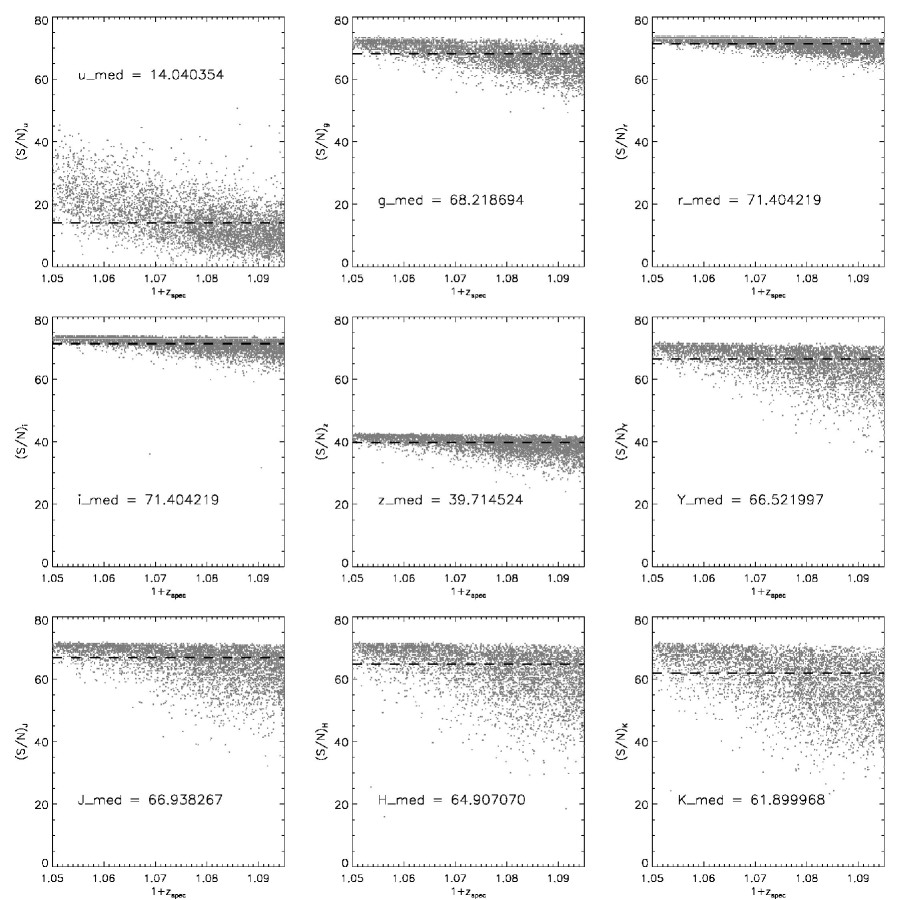
Figure 5: Signal-to-noise ratios (S/N) for the optical+NIR sample. The S/N in the u-band is too low to allow the fitting of galaxy images with Sersic models (as in previous papers in this series; see Section 2.2), so SExtractor was used to obtain the magnitudes and corresponding errors. S/N in all of the other bands is remarkably high. $Dashed$ lines represent the median S/N in each bandpass.

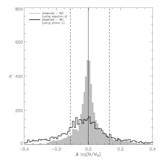
Figure 6: Errors in the stellar mass computed from the observed apparent magnitudes minus the Monte-Carlo magnitudes (see Section 7.1), using the spectro-z (gray) and photo-z (black), for the optical+NIR sample. The $ugrizYJHK$ magnitudes were varied within their 1$\sigma$ errors according to a normal distribution, and the resulting magnitudes were used to scale the template SED to obtain the stellar mass estimate. The solid and dashed lines indicate median and $\pm 2\sigma$ limits, respectively, for the $gray$ histogram.

The photometric measurements of the complete and optical+NIR samples in this study have high S/N ratios (see Figure 5). To investigate the dependence of galaxy stellar mass estimates on photometric errors, we used a Monte-Carlo approach to varying the $ugrizYJHK$ magnitudes. Each magnitude was varied according to a normal distribution, centered on the observed apparent magnitude, using the $1\sigma$ error limits provided by SExtractor. For fixed redshift, the resulting differences in stellar masses from the original sample (optical+NIR) are shown in Figure 6. The masses show a dispersion of $\pm 0.12$ dex at the 95% CL, which lie within uncertainties induced by the photometric redshift, but are surprisingly large given the S/N of this sample, with a negligible systematic bias introduced in the mass.

7.2 Dependence on photometric redshift

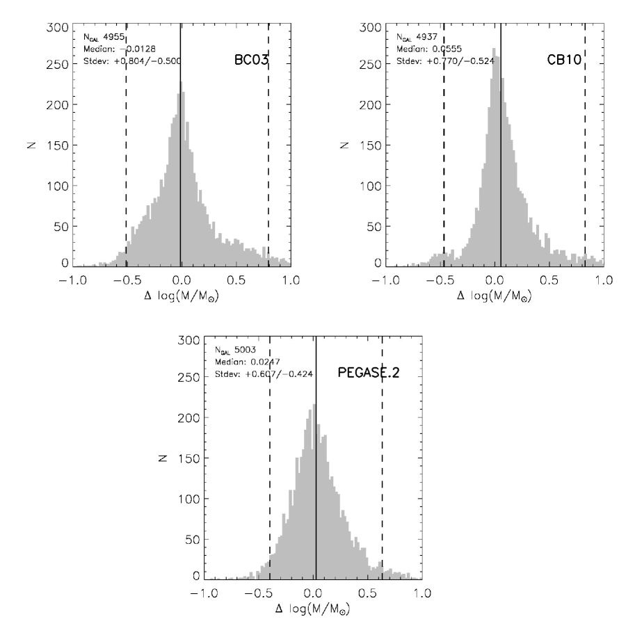
Figure 7: Histograms of $\Delta(\log\mathcal{M})_{s-p}$, defined in Section 6, for spectroscopic and photometric redshifts, using the BC03, CB10, and PEGASE.2 stellar population models. The solid and dashed lines indicate median and $\pm 2\sigma$ limits, respectively. Only objects in the range $9<\log\mathcal{M}/\mathcal{M}_{\sun}<12$ are included in this figure.

We quantified how the stellar mass accuracy is affected by the use of a photometric redshift, which is the typical case for a large imaging survey. Figure 7 shows the difference between the stellar masses computed with the spectroscopic vs. photometric redshifts. The sample uses the entire redshift range $0.05\leq z\leq 0.095$, and all bands are used to scale the mass. We find a median difference of $\sim$0.01 dex, with errors of $+0.804$/$-0.500$ dex at the 95% CL, using BC03 models. This scatter is slightly larger than the systematic uncertainties expected (0.2 dex at the 68% CL) in the stellar mass estimate due to photometric redshifts (Pozzetti et al., 2007; Longhetti & Saracco, 2009) at low redshift . For the optical+NIR sample, the average positive 2$\sigma$ limit on the photo-z is roughly 40% – at the largest redshift ($z=0.095$, i.e. $d_{L}=435$ Mpc), this yields a luminosity distance error of nearly 200 Mpc, or a stellar mass error (from Equation 5) of $\sim$0.4 dex. The photo-z also impacts the template best fit ages differently, depending on stellar population model. We concluded that the unusually low redshift of our sample results in abnormally large mass errors (compared to those reported in the literature) due to the use of photo-zs, since the fractional errors in the luminosity distances are large. For all remaining tests, we use the spectroscopic redshifts.

7.3 Dependence on stellar population model

The comparison of stellar masses between different models is shown in Figures 8 and 9 (see top-left panels). To allow a meaningful comparison with BC03/CB10 and PEGASE.2 models, here we include only objects in the optical+NIR sample that are fit with a solar metallicity ($N_{BC03}=3,371$, $N_{CB10}=4,240$) . The stellar mass comparisons between models yield small offsets. CB10 models produce slightly higher masses by about 0.005 dex, with a scatter of $\sim$0.14 dex with respect to BC03 masses using the spectroscopic redshift (see Table 4). This result seems to be in disagreement with, instead, BC03 models having systematically higher NIR $\mathcal{M}_{*}/\mathcal{L}$ than CB10 models, at given age and metallicity (see e.g. Eminian et al., 2008). Indeed, $LePhare$ gives lower photometric ages when using BC03 (see Figure 3), resulting in lower $\mathcal{M}_{*}/\mathcal{L}$ ratios when compared to CB10 results. This might compensate for any variation of $\mathcal{M}_{*}/\mathcal{L}$ due to the different treatment of the TP-AGB phase between BC03 and CB10. This seems to hold only for ETGs with old ages, as Muzzin et al. (2009) actually found CB10 (as of 2008) based stellar masses to be systematically smaller than those obtained from BC03 for high-redshift ($z\sim 2.3$) galaxies. Moreover, van der Wel et al. (2006) reported that, for $z\sim 0$ galaxies, including the TP-AGB phase, as done in Maraston (2005) stellar population models, leads to lower stellar masses than those obtained with BC03, when fitting both optical and NIR broad-band colors, more consistent with what is reported here. On the other hand, PEGASE.2 models produce systematically lower masses than BC03/CB10. The offsets in these comparisons are likely due to the different prescriptions for the luminous stars dominating the $K$-band flux, and are comparable to other factors discussed below. Longhetti & Saracco (2009) measure the effect of different TP-AGB prescriptions (assuming these stars dominate the $K$-band flux) between stellar population models on the resulting stellar mass when the age is known, finding agreement within at least 20%, between BC03, CB10, and PEGASE.2 models.

Earlier studies (Pozzetti et al., 2007; Treu et al., 2010) find that a Chabrier IMF underestimates galaxy stellar masses by nearly a factor of 2, compared to those derived with the Salpeter IMF. Cappellari et al. (2006) used different models than these authors and find that galaxy stellar masses based on a Salpeter IMF were in some cases too high compared to those determined with stellar kinematics, reaching the same conclusion. We use the stellar population models of BC03/CB10 to further compare model dependent stellar masses (with star-formation histories, metallicities, and color excesses given in Table 1), using different IMFs. Figures 8 and 9 show the dispersion in $\Delta(\log\mathcal{M})$ between the Chabrier and Salpeter IMFs (see top-right panels). The zero-point offset is $-0.227$ ($-0.225$) dex using BC03 (CB10) models, or a factor of $\sim$2, which differs from the analytical estimate (see Appendix B) by $\sim$0.1 dex.

7.4 Dependence on photometric bandpasses fitted

Here we highlight the systematic effects of band scaling in the $\chi^{2}$-minimization as well as inclusion of ultraviolet and NIR continua, separately, in the SED fitting. Again, we remind the reader that these results apply specifically to a low redshift population of ETGs, where the continuum levels behave differently with redshift for ETGs and especially for other morphological types.

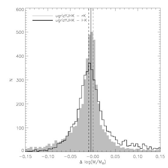
Figure 10: Effect of using different optical+NIR bandpasses for scaling the SED (using BC03). With known redshift, this histogram suggests that there is no systematic bias in choosing all bands as opposed to $K$-band to scale the SED. The median difference (solid vertical) is indistinguishable from zero at the $0.3\sigma$ level (dashed vertical). Note that LePhare does not accept only 1-band for scaling when the redshift is unknown.

In Figure 10, we plot the differences in galaxy stellar mass for several choices of band scaling – $ugrizYJHK$, $rK$, and $HK$. For our optical+NIR sample of low redshift ETGs, this allows for a measurement of the sensitivity of the overall luminosity scaling of the SED to magnitude errors, specifically targeting the $K$-band. The median, dispersion, kurtosis, and skewness for these stellar mass differences are given in Table 3, suggesting that there is a systematic bias in the stellar mass of 0.005 dex when using all bands as opposed to using only the $H$ and $K$ bands. The differences are sharply peaked around zero, as indicated by the high excess kurtosis.

Table 3: Characteristics of $\Delta(\log\mathcal{M})$ for $ugrizYJHK-xK$ (with $x=r,H$) band scaling.

	Median${}^{+2\sigma}_{-2\sigma}$	Kurtosis	Skewness
$ugrizYJHK-rK$	$-8.000$E-$3^{0.06041}_{0.09934}$	9.09	-0.734
$ugrizYJHK-HK$	$-4.500$E-$3^{0.09971}_{0.04286}$	5.61	1.00

These offsets are small compared to errors introduced by other factors explored later in this paper. The excess of positive residuals for $ugrizYJHK-HK$ scaling is possibly due to a known poor modeling effect in the near-infrared described in Sections 5 and 7.3, which predicts $K$-band magnitudes that are too faint. Therefore, we use all bands to measure the stellar mass, so that the scale factor is less sensitive to errors in any one given band. In the minimization, the best $\chi^{2}$ at each redshift step is saved to build the function $F(z)=\exp[-\chi_{min}^{2}(z)/2]$. This function is used to refine the photo-z solution with a parabolic interpolation (Bevington, 1969).

7.5 Dependence on inclusion of rest-frame UV photometry

We use the optical+NIR sample to compare stellar masses computed with and without u-band data, for BC03/CB10 models. We find scatters of $\sim$0.14 and $\sim$0.12 dex, respectively, in $\Delta(\log\mathcal{M})$, as shown in Figures 8 and 9, with negligible systematic bias in the mass (see green histograms in bottom-right panels). Conroy & Gunn (2010) describe the influence of the 4000Å break (quantified as D_n4000) on $ugr$ colors for red sequence galaxies and find that BC03 models, among others, predict D_n4000 strengths that are generally too large. It is possible that this effect, which alone would yield older stellar ages in the $\chi^{2}$-fitting, competes with the underpredicted NIR luminosities to produce the scatter observed in Figure 8 (for $u-$no-$u$). This uncertainty would be difficult to quantify, as these models suffer in reproducing the age-metallicity plane found from spectral fits. However, with the modifications in CB10 models affecting spectra redward of $\sim$6000Å, the $u-$no-$u$ stellar mass differences in Figure 9 have a lower systematic bias and dispersion than the BC03 models, showing that CB10 treats optical+NIR spectral regions more consistently with the observations. Hence, including $u$-band data simply provides more robust stellar mass estimates.

7.6 Dependence on rest-frame NIR photometry

We also test the absence of near-infrared data on the stellar mass estimate (see bottom-right panels of Figures 8 and 9). The $\Delta(\log\mathcal{M})$ offset in $ugrizYJHK-ugriz$ stellar masses is approximately $-0.057\pm 0.10$ ($-0.042\pm 0.12$) dex for BC03 (CB10) models, with $ugriz$-only photometry producing higher stellar masses in both cases. Pozzetti et al. (2007) find a similar result – that is, higher masses by $\sim$0.1 dex using optical-only photometry – for their $K$-selected spectroscopic sample of high redshift galaxies. Given the changes in TP-AGB evolution between BC03/CB10 models, these relatively smaller dispersions suggest that the 4000Å break is a more sensitive constraint in the SED fits than is the continuum level of the NIR data for this sample of low redshift ETGs.

7.7 Dependence on interstellar extinction

We compare stellar masses derived using the Cardelli et al. (1989) and Calzetti et al. (2000) extinction laws with $E(B-V)$ values listed in Table 1. These empirical laws are line-of-sight dependent with average $R_{V}$ equal to $3.1$ and $4.05\pm 0.80$, respectively, in popular photometric redshift codes (e.g. $BPZ$, $HyperZ$, LePhare). Using BC03 models, this mass difference yields errors of $+0.07$/$-0.14$ dex for the optical+NIR sample with negligible systematic bias in the mass. These extinction laws produce excellent mass agreement, however, using CB10 models, which might be related to the fact that CB10 models provide SEDs that are more consistent with the observations in both the optical and NIR. We also measure stellar masses using the Charlot & Fall (2000) extinction law, which is provided with the $GALAXEV$ code and requires as inputs the total effective $V$-band optical depth $\tau_{V}$ and the fraction $\mu$ of it contributed by the interstellar medium. The default values of $\tau_{V}=1.0$ and $\mu=0.3$ are assumed for this test, where it should be noted that these values best describe a population of star-forming galaxies. Our optical+NIR sample yields a $\Delta(\log\mathcal{M})$ zero-point offset of $-0.10$ dex for BC03 models, with CB10 models producing slightly better agreement. Note that this difference is comparable to the offsets found by Ilbert et al. (2010) for the $z\sim 1$ zCOSMOS sample ($\Delta(\log\mathcal{M})_{\mathrm{(Calzetti}-\mathrm{CF2000)}}$ is $-0.14$ dex), where they also show that this systematic offset is larger for massive galaxies with a high SFR.

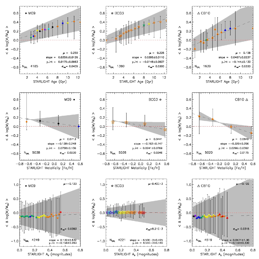
Figure 11: Plots showing $\log\mathcal{M}_{fixed}-\log\mathcal{M}_{free}$ offsets, described in Section 6, as a function of spectroscopically determined age, metallicity, and extinction for the optical+NIR sample, using M09 ($left$), BC03 ($center$), and CB10 ($right$) models. The color code is – from red to blue – # galaxies $<50$, $<100$, $<200$, $<300$, $<400$, $<500$, $<600$ (black $>600$). Measurements in a given bin are only considered if the bin contains $\geq$40 galaxies without catastrophic fitting failures (as returned by $LePhare$). Overplotted are linear fits to each data set. The error bars denote the 95% CL on the median, normalized by the square root of the number of galaxies in the given bin. Provided within each plot are the mean offset ($\mu$), the standard deviation of the residuals ($\sigma_{\mathrm{res}}$), and the slope and y-intercept for a model line fit from a $\chi^{2}$-minimization.

Finally, we utilize spectroscopic measurements of $A_{V}$ (from STARLIGHT) and the Cardelli et al. (1989) extinction law to constrain the interstellar extinction for each galaxy. In LePhare, we fix the color excess $E(B-V)$ based on the relationship $E(B-V)=A_{V}/R_{V}$. We find that for our optical+NIR sample, the uncertainties in the stellar mass estimate due to unknown extinction are comparable ($\sim$0.2 dex for BC03) to the effect of using different extinction laws. However, M09/CB10 models yield much larger uncertainties of $\sim$0.4 dex. We find a negligible systematic trend in mass difference as a function of spectroscopically determined extinction for all models. Figure 11 shows however that when fixing the extinction to the spectroscopic value measured from M09/CB10 models, stellar masses are systematically lower than the free parameter case by $\sim$0.15 dex for all $A_{V}$ values. A linear regression fit to the trend of $\Delta(\log\mathcal{M})$ offset with amount of extinction (in magnitudes) produces

$$\Delta(\log\mathcal{M})=\left\{\begin{array}[]{ll}(0.132\pm 0.832)A_{V}+(-0.156\pm 0.263)&\mathrm{for}~{}\mathrm{M09},\\ (-6.50\mathrm{E-}3\pm 0.425)A_{V}+(8.54\mathrm{E-}3\pm 0.140)&\mathrm{for}~{}\mathrm{BC03},\\ (0.0471\pm 1.30)A_{V}+(-0.132\pm 0.330)&\mathrm{for}~{}\mathrm{CB10}\\ \end{array}\right.$$ (6)

where the 1$\sigma$ uncertainties on the regression coefficients are provided above. Large uncertainties in $\Delta(\log\mathcal{M})$ affect the reliability of this fit, but it is provided for reference.

Fitting broadband photometry seems to produce lower interstellar extinction than spectral fitting for our sample of ETGs, as shown in the right panels in Figure 4. This would lower the $0.4\times m_{\lambda^{\prime}}$ term in Equation 5 and produce a higher stellar mass estimate. We note here that we do not provide a mass correction analysis as a function of photometrically determined extinction, due to the shallow trend in $\Delta(\log\mathcal{M})$ with $A_{V}$. Furthermore, the $A_{V}$ (or equivalently $E(B-V)$) parameter space cannot be specified directly within the STARLIGHT $\chi^{2}$-fitting.

7.8 Dependence on stellar age and metallicity

This section spotlights both the effect of different best fit ages and metallicities on the resulting stellar masses, and suggests how blue continuum fluxes and mass-to-light ratios could explain the large stellar mass differences due to photometrically determined ages. To this end, we have used optical spectra to constrain independently age and metallicity in the models.

7.8.1 Dependence on stellar metallicity

The Padova 1994 stellar evolutionary tracks used by BC03/CB10 encompass six metallicities in the range $Z/Z_{\sun}=0.005-2.5$, with the four most metal-rich models chosen for this study. The M09 model fits use $Z/Z_{\sun}=0.2,0.4,1.0,1.6$ metallicities from the Padova 2000 library. We separate galaxies on the basis of the metallicity ranges given in Table 1 and run LePhare with the metallicity constrained to the closest value. The result is a systematic offset for unknown metallicity consistent with zero for most objects fit with M09 models. However, metallicity is more poorly constrained with BC03/CB10 models, yielding a larger systematic offset in the stellar mass, with uncertainties as high as $\sim$0.2 dex at low metallicity (see Table 4). The linear regression fit to our optical+NIR sample yields the following functional form:

$$\Delta(\log\mathcal{M})=\left\{\begin{array}[]{ll}(-0.138\pm 0.248)Z+(0.0758\pm 0.136)&\mathrm{for}~{}\mathrm{M09},\\ (-0.162\pm 0.147)Z+(0.0241\pm 0.0769)&\mathrm{for}~{}\mathrm{BC03},\\ (-0.320\pm 0.206)Z+(0.0296\pm 0.0362)&\mathrm{for}~{}\mathrm{CB10}\\ \end{array}\right.$$ (7)

where the 1$\sigma$ uncertainties on the regression coefficients are provided above. Large uncertainties in $\Delta(\log\mathcal{M})$ for the non-solar metallicity models affect the reliability of this fit, but it is provided for reference.

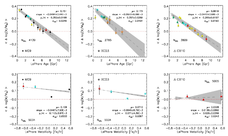
Figure 12: The mass correction, $\epsilon$, plots as a function of photometrically determined age and metallicity, using M09 ($left$), BC03 ($center$), and CB10 ($right$) models. The color code is defined in Figure 11. Measurements in a given bin are only considered if the bin contains $\geq$20 galaxies without catastrophic fitting failures (as returned by $LePhare$). Overplotted are linear fits to each data set. The error bars denote the 95% CL on the median, normalized by the square root of the number of galaxies in the given bin. Provided within each plot are the mean offset ($\mu$), the standard deviation of the residuals ($\sigma_{\mathrm{res}}$), and the slope and y-intercept for a model line fit from a $\chi^{2}$-minimization.

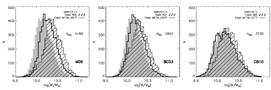
Figure 13: Stellar mass distributions for the optical+NIR sample. Only the spectroscopic redshift is constrained in the $gray$ histogram. The $black$ $shaded$ ($outlined$) histograms show the stellar masses, corrected for age (metallicity) according to the procedure described in Section 7.8.2. These corrections utilize the spectroscopic measurements from M09 ($left$), BC03 ($center$), and CB10 ($right$) stellar population models, respectively.

We can see how the distribution of stellar masses changes for our sample by applying an offset to each mass as a function of its photometrically determined metallicity, which we call the mass correction, $\epsilon$. For galaxies with a given photometrically-determined metallicity, we add an offset calculated from the linear fit in Figure 12 to the stellar mass measured with only the spectroscopic redshift constrained. Figure 13 shows the distribution of stellar masses for our optical+NIR sample, corrected for these offsets. This technique shows that the median stellar mass changes by $\sim$0.1 dex when using the M09/BC03 models. The distribution remains more consistent in CB10 models, which may be expected given the slightly better agreement between spectroscopic and photometric metallicities using these templates (see CB10/Metallicity plot in Figure 4).

7.8.2 Dependence on stellar age

As described in Section 7.3, stellar masses of low redshift ETGs have uncertainties of $\sim$0.14 dex at the 95% CL due to the stellar population models alone. Furthermore, the photometrically determined stellar age is model-dependent. The relationship between dominant stellar population age and stellar mass is not easily quantifiable, but errors in the age are propagated to errors in the mass estimate. To this end, we have used stellar age measurements from STARLIGHT spectral fits to fix the age of the template used in the $\chi^{2}$-minimization.

Figure 11 shows an estimate of the systematic bias in stellar mass for unconstrained age plotted as a function of spectroscopically determined age. We note that when constraining the stellar age in LePhare to its spectroscopically determined value, only 1,314 (1,810) galaxies, using BC03 (CB10) models, have non-zero $\exp(-\chi^{2}/2)$ values. There is a clear trend of increasing mass difference with age. Furthermore, using BC03 models in the SED fitting (provided spectroscopic constraints separately from M09/BC03) yields systematically lower stellar masses at all ages. This trend is also evident from CB10 models, though stellar masses for unconstrained age are systematically higher below about 4 Gyr. The linear regression fit to the optical+NIR sample yields the following functional form:

$$\Delta(\log\mathcal{M})=\left\{\begin{array}[]{ll}(0.0359\pm 0.0126)t+(0.0175\pm 0.0963)&\mathrm{for}~{}\mathrm{M09},\\ (0.0395\pm 0.0110)t+(-0.0148\pm 0.0837)&\mathrm{for}~{}\mathrm{BC03},\\ (0.0467\pm 0.0237)t+(-0.144\pm 0.133)&\mathrm{for}~{}\mathrm{CB10}\\ \end{array}\right.$$ (8)

where the 1$\sigma$ uncertainties on the regression coefficients are provided above. Notice that there is a significant positive trend in stellar mass underestimation with increasing age that is well approximated by the linear model.

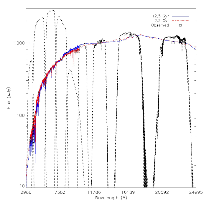
Figure 14: Best-fit output spectra from LePhare for a single galaxy with age fixed to the spectroscopic value of 12.5 Gyr (solid blue) and photometrically fit to 2.2 Gyr (dash-dot red), selected from the optical+NIR sample. The observed apparent magnitudes, converted in flux, are overplotted (squares) with their 1$\sigma$ errors. The $ugrizYJHK$ filter curves are overplotted for reference.

This gross underestimate in mass for old stellar populations might be due to the fact that models underestimate the ages – possibly because of age-metallicity-extinction degeneracy or a failure of the models to reproduce the observed spectra – and then the SED fitting code increases the luminosity scale factor accordingly. To illustrate this, we select a single galaxy with spectroscopically and photometrically determined ages of 12.5 Gyr and 2.2 Gyr, respectively, and compare the best fit redshifted, reddened photometric SEDs for free and fixed age (see Figure 14), where the fixed age stellar mass is higher by $\sim$0.42 dex. The galaxy is best fit by a $Z/Z_{\sun}=0.4$ metallicity, and differs by 0.1 in $E(B-V)$, using BC03 models. Following Equation 5, the median difference in $0.4\times m_{\lambda^{\prime}}$ in the $g$-band is 0.06 mag (with higher flux in the 2.2 Gyr SED) and indistinguishable from our broadband photometry alone. Older and younger populations have very different stellar mass-to-light ratios, where for instance the difference in $\log(\mathcal{M}_{*}/\mathcal{L}_{B})$ for the two best fit ages here is $\sim$0.67 dex (with lower $B$-band mass-to-light ratio in the 2.2 Gyr SED). As expected, the 4000Å break is the most significantly differing feature in the broadband colors of these SEDs, with $\Delta[\log(\mathcal{M}_{*}/\mathcal{L}_{B})]-\Delta(0.4\times m_{g})$ accounting for most of the measured difference in stellar mass for this particular object, yet it cannot be photometrically distinguished despite the high S/N of our objects at this redshift . Furthermore, including the $K$-band photometry seems to bias most SEDs towards young ages, assuming our ellipticals are indeed dominated by older stars. So, we can attribute larger differences in the stellar mass due to unknown age to the blue $\mathcal{M}_{*}/\mathcal{L}$ for different stellar population ages. It is also true that differing spectroscopic and photometric metallicities will produce different stellar masses, but given the trends provided in Section 7.8.1, it is likely that large differences in age dominate the effect of age-metallicity degeneracy on the galaxy stellar mass.

We can see how the distribution of stellar masses changes for our sample by applying an offset to each mass as a function of its photometric age, similar to the procedure described at the end of Section 7.8.1. Figure 13 shows the distribution of stellar masses for our optical+NIR sample, corrected for these offsets. This technique shows that the median stellar mass changes by as much as $\sim$0.1 dex when using the updated CB10 models.

8 External comparison of stellar masses

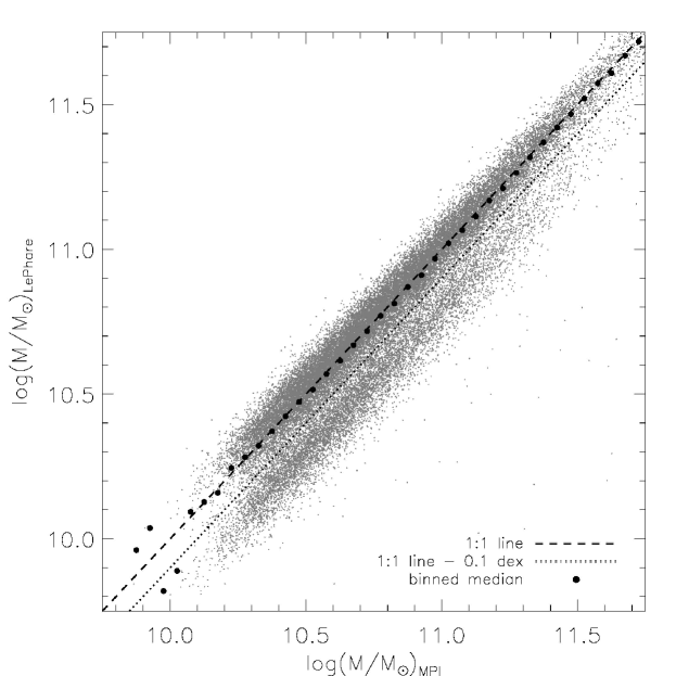
Figure 15: Comparison of total stellar masses for the complete sample and the same sample of galaxies from a group at the Max Planck Institute (obtained from http://www.mpa-garching.mpg.de/SDSS/DR7/Data/stellarmass.html), who use SDSS FiberMag photometry. The black circles are obtained by median-binning the data, the dashed line is the 1:1 line, and the dotted line is arbitrarily drawn 0.1 dex below the 1:1 line to separate the two trends observed here.

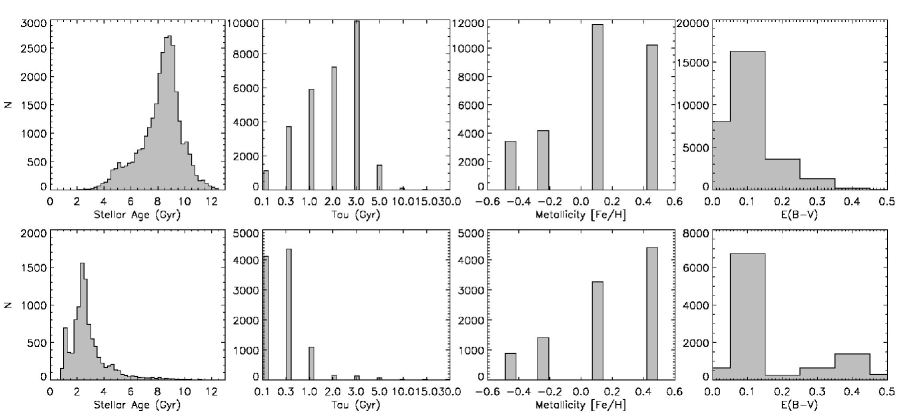
Figure 16: Distributions of age, star-formation decay time scale, metallicity, and extinction for galaxies lying above (top panels) and below (bottom panels) the dotted line in Figure 15.

As a comparison to related work, we plot stellar masses obtained from our SED fits against those derived from a group at the Max Planck Institute (see Figure 15), using the complete sample and BC03 stellar population models . We convert to total stellar mass by dividing each set of measured stellar masses by an aperture correction, corresponding to the fraction of $z$-band light contained within the $i$-band Kron aperture (LePhare) and the SDSS fiber (MPI). This procedure assumes that the stellar mass in a galaxy is distributed in the same way as the $z$-band light. We notice two trends in this comparison, with $\sim$75% of the galaxies lying above an arbitrary line drawn 0.1 dex below the 1:1 line. The subset of galaxies that lie above this line are in excellent agreement with those from MPI, with a negligible offset and 2$\sigma$ uncertainty of $\sim$0.1 dex, likely due in part to the difference between how Kron and SDSS FiberMags are measured (e.g. correcting the latter for emission lines) as well as potential differences in model parameters. The distributions of best fit age, star-formation decay time scale, metallicity, and extinction are plotted in Figure 16 for galaxies lying above (top panels) and below (bottom panels) the dotted line drawn in Figure 15. We see that with metallicity and extinction being similar for the two samples, the contribution from a high $t/\tau$ is a redder galaxy – that is, such a galaxy has enough e-folding times to allow the younger stars to fade. This produces a degeneracy in the shape of the SEDs, as compared to a similar $t/\tau$ for an older galaxy, resulting in a lower mass for the younger SED. We have directly verified this degeneracy for several objects with similar $t/\tau$, metallicity, extinction, and redshift, but different ages.

We also compared the stellar masses that we present here with those presented in Paper IV, finding trends similar to those described above. Specifically, we find a negligible offset (0.003 dex) with a modest 2$\sigma$ scatter of $\sim$0.1 dex for galaxies (65%) lying above a line, drawn similarly to the dotted line in Figure 15. The stellar population model differences between the stellar masses presented in this paper – i.e. for BC03 models, with a Chabrier IMF, Cardelli extinction law, and spectroscopic redshift – and those presented in Paper IV is the permitted model decay time scales for star-formation ($\tau$), where in this paper we also include $\tau=0.1,0.3,\mathrm{and}~{}30.0$ Gyr models, and use of the Calzetti law in Paper IV (which induces negligible offset in the stellar mass). Another difference is that in this paper we use all available bands to scale the SED, so that the scale factor is less sensitive to errors in any one given band. In Paper IV, we used only $K$-band to scale the SED, due to its supposed independence from the effects of dust extinction and young, luminous stars (see Section 4.1).

9 Summary & conclusions

We measured systematic errors in galaxy stellar masses due to different ingredients in widely used models from stellar population synthesis techniques. Using a large sample of high S/N, low redshift ETGs, we want to accomplish two primary goals

– Determine at a high-level of significance, the statistical biases and uncertainties inherent in a stellar mass estimate;

– Provide robust corrections to a sample of photometrically determined galaxy stellar masses, when spectroscopy is unavailable.

We first presented a comparison of BC03, CB10, and PEGASE.2 stellar mass estimates, finding that masses have dispersions of $\sim$$0.10-0.15$ dex at the 95% CL, with this uncertainty arguably being due to the different treatment of the TP-AGB stellar evolutionary phase. In general, our tests find no statistically significant systematic mass bias at the $2\sigma$ level due to variations of the stellar population models, extinction laws, and photometric bandpasses. This includes varying scaling bandpasses in the fitting technique as well as the magnitudes used in generating the photometric SED. However, a systematic offset of about $-0.23$ dex (inconsistent with zero at the $2\sigma$ level) is observed between stellar masses predicted from Chabrier and Salpeter IMFs. The newer TP-AGB calculations by Marigo & Girardi (2007) affecting $K$-band magnitudes also improve the quality of $u$-band fits, where the dispersion in galaxy stellar mass measured with and without $u$-band data is improved by nearly 20% from BC03 to CB10 models. It is interesting to note that stellar mass estimates are more consistent with no near-infrared photometry than they are without $u$-band data, at least using BC03 models with this sample of ETGs.

The observed systematic stellar mass biases and dispersions for our optical+NIR and complete sample of ETGs are summarized in Table 4. As expected for this redshift range, using the photo-z produces the largest systematic uncertainties in the stellar mass estimate. We find that a Chabrier (2003) IMF produces lower stellar masses than a Salpeter (1955) IMF by about 0.227 (0.225) dex for BC03 (CB10) models, in agreement with other studies, but lower by about 0.1 dex than the difference predicted by direct integration of the formulae over the mass range 0.1$-$100 $\mathcal{M}_{\sun}$ (Appendix B). For the optical+NIR sample, this difference falls within the 3$\sigma$ confidence limits of the observational estimate (i.e. 0.23 +0.15/-0.10 for BC03), while for the complete sample, it is within the 4$\sigma$ confidence limits for BC03 and highly inconsistent with zero ($>4\sigma$ deviation) for CB10.

An important part of this work is the investigation of systematic effects on the photometrically determined stellar mass when spectroscopic constraints on age, metallicity, and extinction are unavailable, and to provide statistically robust stellar mass corrections as a function of these photometric parameters for low redshift early-type galaxies. We used 5,068 objects with $ugrizYJHK$ photometry and spectroscopy to achieve this goal. Offsets from extinction constraints are the smallest of these systematic effects; this implies that the SED fitting is less sensitive to the coarse extinction grid employed by stellar population models when estimating the stellar mass. We find a negligible trend with $A_{V}$ in stellar mass difference for the optical+NIR sample. However, there is about a 0.15 dex bias towards higher masses for all extinctions when $A_{V}$ is unknown, using M09/CB10 models. The dispersion in these mass differences is about $\pm 0.5$ dex (consistent with zero), slightly lower for BC03 models, yet larger than uncertainties introduced by unknown age/metallicity, mainly because of the smaller number of galaxies in a given extinction bin. Fitting broadband photometry seems to produce lower interstellar extinction than spectral fitting for our sample of ETGs, as shown in the right panels in Figure 4. This would lower the $0.4\times m_{\lambda^{\prime}}$ term in Equation 5 and produce a higher stellar mass estimate. We comment that for general surveys, it might be more appropriate to fit an SED with one extinction law (e.g. Calzetti et al., 2000), and then refit with a more appropriate law once an approximate age is established.

The positive trend in $\Delta(\log\mathcal{M})$ with increasing metallicity is simply a result of the inverse trend shown in the middle panels of Figure 4. That is, spectral fits on average produce lower metallicities than broadband photometric SED fitting for these objects; and for any given age, a lower metallicity SSP has a lower mass. This is merely a reflection of the failure of such a coarse metallicity grid to constrain the model in the SED fitting, as expected. Dressler & Shectman (1987) show that the size of the 4000Å break in spheroidal galaxies is quite insensitive to metallicity, so even provided a wider range of stellar population metallicities, our result should remain unchanged in this regard for (old) ETGs. We chose a larger grid of stellar ages for M09/BC03/CB10 models, ranging from $0.5-12.5$ Gyr to constrain age in the $\chi^{2}$-minimization. We measure remarkably lower stellar masses when age is unknown for all young/old populations (except $\lesssim 4$ Gyr for CB10 models), with uncertainties of around $0.2-0.3$ dex. Indeed, for our low redshift ETGs with older stellar populations, we would be underestimating the stellar mass content by a factor of 2 (for galaxies with $t\sim 10$ Gyr from BC03/CB10 models). We can argue that the increasing trend with stellar age in Figure 11 is directly due to the overall underestimate in photometrically determined age for all models (see left panels of Figure 4), whereas we argue in Section 7.8.2, a difference of $\sim$0.7 dex in the best fit age can yield a stellar mass difference of $\sim$0.4 dex, explained by varying $\mathcal{M}_{*}/\mathcal{L}$ ratios between different stellar age SEDs. Notice that unknown ages, resulting from a mismatch between the true star formation history of a galaxy and the simplified form used in SED fits (e.g. an exponentially declining SFR), can also affect significantly the stellar mass determination of high-redshift galaxies, as discussed, e.g., by Pozzetti et al. (2007) and Lee et al. (2010).

In conclusion, we find uncertainties in the galaxy stellar mass due to different stellar population models, IMFs, and extinction laws that are much less than uncertainties introduced by using the photo-z over this small redshift range. More notable are offsets measured between Chabrier/Salpeter IMFs, Cardelli/CF2000 extinction laws, and changes in TP-AGB evolutionary prescriptions – between CB10/PEGASE.2 models. The discrepancies in ages, metallicities, and extinctions between spectroscopic and photometric measurement techniques propagate to uncertainties in the stellar mass estimates, yielding notably lower masses when stellar age is unknown. Given the coarse grid of stellar metallicities, the age-metallicity degeneracy is likely to contribute to the large discrepancies in spectroscopic and photometric measurements. Finally, we proposed a mass correction to our sample that incorporates these systematic offsets as a function of their photometrically determined age and metallicity, finding that the sample median mass increases by a factor of roughly 1.3. We would like to comment that these results apply to optical and near-infrared broadband photometry of low redshift ETGs. Detailed quantification of the systematic errors involved in SED fitting have produced results consistent with what other studies have found and have allowed us to obtain consistent stellar mass estimates for this sample.

We have used data from the 4th data release of the UKIDSS survey, which is described in detail in Warren et al. (2007). The UKIDSS project is defined in Lawrence et al. (2007). UKIDSS uses the UKIRT Wide Field Camera (WFCAM; Casali et al. (2007)). The photometric system is described in Hewett et al. (2006), and the calibration is described in Hodgkin et al. (2009). The pipeline processing and science archive are described in Irwin et al. (2011, in prep) and Hambly et al. (2008). Funding for the SDSS and SDSS-II has been provided by the Alfred P. Sloan Foundation, the Participating Institutions, the National Science Foundation, the U.S. Department of Energy, the National Aeronautics and Space Administration, the Japanese Monbukagakusho, the Max Planck Society, and the Higher Education Funding Council for England. The SDSS Web Site is http://www.sdss.org. The SDSS is managed by the Astrophysical Research Consortium for the Participating Institutions. The Participating Institutions are the American Museum of Natural History, Astrophysical Institute Potsdam, University of Basel, University of Cambridge, Case Western Reserve University, University of Chicago, Drexel University, Fermilab, the Institute for Advanced Study, the Japan Participation Group, Johns Hopkins University, the Joint Institute for Nuclear Astrophysics, the Kavli Institute for Particle Astrophysics and Cosmology, the Korean Scientist Group, the Chinese Academy of Sciences (LAMOST), Los Alamos National Laboratory, the Max-Planck-Institute for Astronomy (MPIA), the Max-Planck-Institute for Astrophysics (MPA), New Mexico State University, Ohio State University, University of Pittsburgh, University of Portsmouth, Princeton University, the United States Naval Observatory, and the University of Washington. The authors would also like to thank Olivier Ilbert and Stephane Arnouts for help with using $LePhare$.

Table 4: Summary of results: optical+NIR. Offset is the median of the $\Delta(\log\mathcal{M})$ histograms and $2\sigma$ is the $\pm$2-sigma uncertainty on the median. Offset is provided for the fixed$-$free parameter tests (Figure 11) at the median spectroscopic values of $t$, Z, and $A_{V}$ for BC03 and CB10 models. Unless otherwise noted, these tests assume a spectroscopic redshift, Chabrier IMF, and Cardelli extinction law. Note that galaxies fit with the median spectroscopic age of 4.0 Gyr (CB10) suffered catastrophic fitting failures, and so the offset and uncertainties are reported here for an age of 4.5 Gyr.

	BC03		CB10
	Offset	$2\sigma$	Offset	$2\sigma$	Note
spectro-z $-$ photo-z	0.0128	+0.804/-0.500	0.0555	+0.771/-0.524	$0.000\leq z_{p}\leq 0.300$, $9<\log\mathcal{M}/\mathcal{M}_{\sun}<12$
BC03 $-$ CB10	-4.64E-3	+0.118/-0.163	-4.64E-3	+0.118/-0.163	STELIB spectral library
BC03 (CB10) $-$ PEGASE.2	0.0962	+0.0837/-0.112	0.0858	+0.0934/-0.132	—
Chabrier $-$ Salpeter	-0.227	+0.0855/-0.0323	-0.225	+0.0441/-0.0281	STELIB spectral library
Cardelli $-$ Calzetti	-4.50E-3	+0.0711/-0.140	-1.00E-4	+0.109/-0.0375	Cardelli/Calzetti from LePhare code
Cardelli $-$ CF2000	-0.104	+0.142/-0.170	-0.0680	+0.156/-0.131	$\tau_{V}=1.0$, $\mu=0.3$ (in GALAXEV code)
$u-$ no-$u$	-0.0257	+0.131/-0.151	-6.30E-3	+0.115/-0.121	—
$ugrizYJHK-ugriz$	-0.0566	+0.0868/-0.125	-0.0419	+0.147/-0.108	—
Fixed$-$Free
$t$	0.0833	+0.108/-0.144	0.0590	+0.284/-0.201	$t_{med}=3.25~{}(4.50)$ Gyr, BC03 (CB10)
$Z$	0.0587	+0.191/-0.0442	-1.50E-3	+0.0273/-0.151	[Fe/H]${}_{med}=0.0932~{}(0.0932)$, BC03 (CB10)
$A_{V}$	0.0276	+0.280/-0.147	-0.164	+0.554/-0.488	$A_{V,med}=0.12~{}(0.10)$, BC03 (CB10)

Table 5: Summary of results: complete. Offset is the median of the $\Delta(\log\mathcal{M})$ histograms and $2\sigma$ is the $\pm$2-sigma uncertainty on the median. Offset is provided for the fixed$-$free parameter tests (Figure 11) at the median spectroscopic values of $t$, Z, and $A_{V}$ for BC03 and CB10 models. Unless otherwise noted, these tests assume a spectroscopic redshift, Chabrier IMF, and Cardelli extinction law. Again, the reader is cautioned on use of the results in this table, per the reasons outlined in Section 7.

	BC03		CB10
	Offset	$2\sigma$	Offset	$2\sigma$	Note
spectro-z $-$ photo-z	0.0281	+0.780/-0.330	0.0185	+0.772/-0.316	$0.000\leq z_{p}\leq 0.300$, $9<\log\mathcal{M}/\mathcal{M}_{\sun}<12$
BC03 $-$ CB10	0.0131	+0.0424/-0.0326	0.0131	+0.0424/-0.0326	STELIB spectral library
BC03 (CB10) $-$ PEGASE.2	0.0871	+0.0516/-0.0908	0.0802	+0.0550/-0.151	—
Chabrier $-$ Salpeter	-0.233	+0.0144/-0.0140	-0.231	+0.0173/-0.0151	STELIB spectral library
Cardelli $-$ Calzetti	-0.0193	+0.0777/-0.0386	5.10E-3	+0.0578/-0.0718	Cardelli/Calzetti from LePhare code
Cardelli $-$ CF2000	-0.0693	+0.0918/-0.0501	-0.0225	+0.0941/-0.0433	$\tau_{V}=1.0$, $\mu=0.3$ (in GALAXEV code)
$u-$ no-$u$	-0.0128	+0.0410/-0.102	-0.0166	+0.0571/-0.187	—

Appendix A SDSS fiber vs. Kron radius

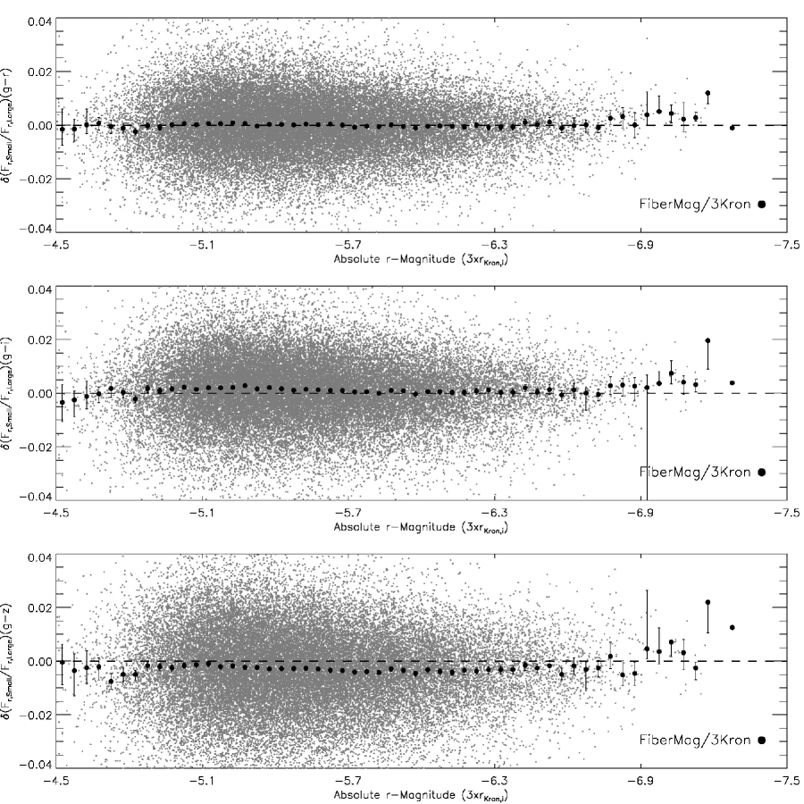
Figure 17: Difference in flux ratio of SDSS FiberMags over Kron magnitudes between the $g$ and $x$ wavebands, with $x=[riz]$, as a function of the absolute $r$-band magnitude for the complete sample of ETGs. Black circles are obtained by median-binning the data, with error bars marking the 2$\sigma$ uncertainty on median values. Notice that there is no variation in the difference of flux ratios from $g$ through $z$, i.e. no significant color gradient between the Fiber and Kron apertures. In $g-z$ there is a small negative offset, but it is less than 0.005 magnitudes.

In this paper, we provide spectroscopic parameters measured within the SDSS fiber radius of $1.5^{\prime\prime}$. However, photometric magnitudes are measured using an adaptive aperture radius of $3\times r_{K,i}$ (see Section 2). Figure 17 shows the difference in flux ratio of SDSS FiberMags to Kron magnitudes between the wavebands $g$ and $x$, with $x=riz$, as a function of $M_{r}$ for the complete sample. The plot shows that there is essentially no color gradient between the $1.5^{\prime\prime}$ and $3\times r_{K,i}$ apertures, from $g$ through $z$. Indeed, the FiberMag/($3\times r_{K,i}$) flux ratios have color consistent with zero inside the $2\sigma$ error bars for most of the absolute magnitude range, with no noticeable dependence on $M_{r}$. We conclude that it is reasonable to compare STARLIGHT spectroscopic parameters, measured within the fiber aperture, to those from SED fitting, measured within the $3\times r_{K,i}$ aperture.

Appendix B The initial mass function (IMF)

Expressions for the initial distribution of stars in a stellar population as a function of mass, known as the stellar initial mass function (IMF), have been proposed by several authors (e.g. Salpeter, 1955; Scalo, 1986; Chabrier, 2003). In this paper, we primarily use the Chabrier IMF for BC03/CB10, parameterized as

$$\xi(m)\propto\left\{\begin{array}[]{ll}\exp[-\frac{(\log m-\log m{{}_{c}})^{2}}{2\sigma^{2}}]&,\mathrm{for}~{}0.1\leq m/\mathcal{M}_{\sun}\leq 1,\\ m^{-2.3}&,\mathrm{for}~{}1<m/\mathcal{M}_{\sun}\leq 100,\\ \end{array}\right.$$ (B1)

with $m_{c}=0.08\mathcal{M}_{\sun}$ and $\sigma=0.69$, and the Scalo IMF for PEGASE.2, approximated here by two power-law segments:

$$\xi(m)\propto\left\{\begin{array}[]{ll}m^{-1.53}&,\mathrm{for}~{}0.1\leq m/\mathcal{M}_{\sun}\leq 1,\\ m^{-2.67}&,\mathrm{for}~{}1<m/\mathcal{M}_{\sun}<120.\\ \end{array}\right.$$ (B2)

The logarithmic slope of $\xi(m)\propto m^{-2.35}$ (B3) for the Salpeter IMF is tested against the Chabrier form in Section 7.3. We can compare the results to the analytical approximations, derived by integrating Equations (B1), (B2), and (B3) as $m\times\xi(m)$. Salpeter masses are expected to be a factor of 2.15 ($\sim$0.33 dex) larger than Chabrier, and Scalo masses are expected to be larger by a factor of 1.05 over Chabrier. The analytical result ($0.33$ dex) falls within the 3$\sigma$ confidence limits of the Chabrier/Salpeter comparison in Figures 8 and 9. We then take the difference in stellar mass between the Chabrier and Scalo IMFs computed above and apply this correction to $\Delta(\log\mathcal{M})$ for BC03(CB10)$-$PEGASE.2, as described in the text.

Table 6: Stellar population model parameters (BC03/CB10/PEGASE.2).

	BC03/CB10		PEGASE.2
	$\tau$
Number	(Gyr)	$Z$	SFR
1	0.1	$0.2\times Z_{\sun}$	$\delta(t=0)$
2	0.1	$0.4\times Z_{\sun}$	$\tau=0.1$
3	0.1	$Z_{\sun}$	$\tau=0.3$
4	0.1	$3\times Z_{\sun}$	$\tau=0.5$
5	0.3	$0.2\times Z_{\sun}$	$\tau=0.7$
6	0.3	$0.4\times Z_{\sun}$	$\tau=1.0$
7	0.3	$Z_{\sun}$	$\tau=2.0$
8	0.3	$3\times Z_{\sun}$	$\tau=3.0$
9	1.0	$0.2\times Z_{\sun}$	$\tau=5.0$
10	1.0	$0.4\times Z_{\sun}$	$\tau=7.0$
11	1.0	$Z_{\sun}$	$\tau=9.0$
12	1.0	$3\times Z_{\sun}$	$\tau=10.0$
13	2.0	$0.2\times Z_{\sun}$	$\tau=15.0$
14	2.0	$0.4\times Z_{\sun}$	$\tau=20.0$
15	2.0	$Z_{\sun}$	$0.5\times 10^{-4}\mathcal{M}_{\sun}Myr^{-1}$
			for $t\leq 20$ Gyr
16	2.0	$3\times Z_{\sun}$	—
17	3.0	$0.2\times Z_{\sun}$	—
18	3.0	$0.4\times Z_{\sun}$	—
19	3.0	$Z_{\sun}$	—
20	3.0	$3\times Z_{\sun}$	—
21	5.0	$0.2\times Z_{\sun}$	—
22	5.0	$0.4\times Z_{\sun}$	—
23	5.0	$Z_{\sun}$	—
24	5.0	$3\times Z_{\sun}$	—
25	10.0	$0.2\times Z_{\sun}$	—
26	10.0	$0.4\times Z_{\sun}$	—
27	10.0	$Z_{\sun}$	—
28	10.0	$3\times Z_{\sun}$	—
29	15.0	$0.2\times Z_{\sun}$	—
30	15.0	$0.4\times Z_{\sun}$	—
31	15.0	$Z_{\sun}$	—
32	15.0	$3\times Z_{\sun}$	—
33	30.0	$0.2\times Z_{\sun}$	—
34	30.0	$0.4\times Z_{\sun}$	—
35	30.0	$Z_{\sun}$	—
36	30.0	$3\times Z_{\sun}$	—

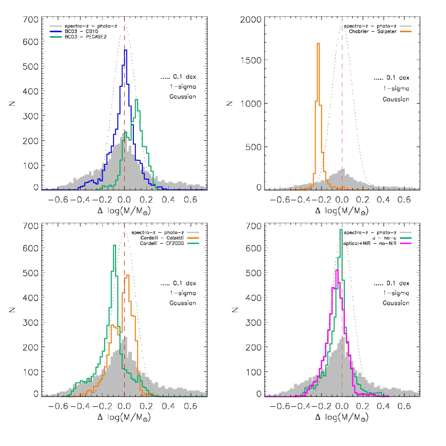
Figure 8: Histograms of $\Delta(\log\mathcal{M})$, defined in Section 6, for the optical+NIR sample and various BC03 model parameters. With the exception of the spectro-z$-$photo-z mass plot (gray), the redshift is fixed in each case. A Chabrier IMF and Cardelli extinction law is assumed, unless otherwise noted. Overplotted are a vertical $dashed$ line and a Gaussian with $\sigma=0.1$ dex centered on zero.

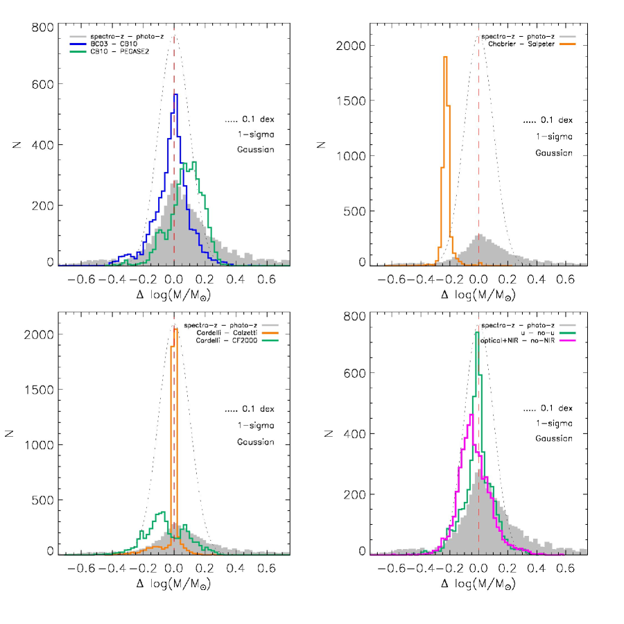
Figure 9: Histograms of $\Delta(\log\mathcal{M})$, defined in Section 6, for the optical+NIR sample and various CB10 model parameters. With the exception of the spectro-z$-$photo-z mass plot (gray), the redshift is fixed in each case. A Chabrier IMF and Cardelli extinction law is assumed, unless otherwise noted. Overplotted are a vertical $dashed$ line and a Gaussian with $\sigma=0.1$ dex centered on zero. A color version of this figure is available online.

References

- Abdalla et al. (2008) Abdalla, F. B., Banerji, M., Lahav, O., & Rashkov, V. 2008, ArXiv e-prints
- Arnouts et al. (1999) Arnouts, S., Cristiani, S., Moscardini, L., Matarrese, S., Lucchin, F., Fontana, A., & Giallongo, E. 1999, MNRAS, 310, 540
- Bell et al. (2003) Bell, E. F., McIntosh, D. H., Katz, N., & Weinberg, M. D. 2003, ApJS, 149, 289
- Benítez (2000) Benítez, N. 2000, ApJ, 536, 571
- Bernardi et al. (2010) Bernardi, M., Shankar, F., Hyde, J. B., Mei, S., Marulli, F., & Sheth, R. K. 2010, MNRAS, 404, 2087
- Bernardi et al. (2003) Bernardi, M., et al. 2003, AJ, 125, 1849
- Bertin & Arnouts (1996) Bertin, E., & Arnouts, S. 1996, A&AS, 117, 393
- Bevington (1969) Bevington, P. R. 1969, Data reduction and error analysis for the physical sciences (New York: McGraw-Hill)
- Blanton et al. (2003) Blanton, M. R., et al. 2003, ApJ, 594, 186
- Bolzonella et al. (2000) Bolzonella, M., Miralles, J., & Pelló, R. 2000, A&A, 363, 476
- Bruzual (2007) Bruzual, A. G. 2007, in IAU Symposium, Vol. 241, IAU Symposium, ed. A. Vazdekis & R. F. Peletier, 125–132
- Bruzual & Charlot (2003) Bruzual, G., & Charlot, S. 2003, MNRAS, 344, 1000
- Bundy et al. (2005) Bundy, K., Ellis, R. S., & Conselice, C. J. 2005, ApJ, 625, 621
- Calzetti et al. (2000) Calzetti, D., Armus, L., Bohlin, R. C., Kinney, A. L., Koornneef, J., & Storchi-Bergmann, T. 2000, ApJ, 533, 682
- Capaccioli et al. (1992) Capaccioli, M., Caon, N., & D’Onofrio, M. 1992, MNRAS, 259, 323
- Cappellari et al. (2006) Cappellari, M., et al. 2006, MNRAS, 366, 1126
- Cardelli et al. (1989) Cardelli, J. A., Clayton, G. C., & Mathis, J. S. 1989, ApJ, 345, 245
- Casali et al. (2007) Casali, M., et al. 2007, A&A, 467, 777
- Chabrier (2003) Chabrier, G. 2003, PASP, 115, 763
- Charlot & Bruzual (1991) Charlot, S., & Bruzual, A. G. 1991, ApJ, 367, 126
- Charlot & Fall (2000) Charlot, S., & Fall, S. M. 2000, ApJ, 539, 718
- Cid Fernandes et al. (2005) Cid Fernandes, R., Mateus, A., Sodré, L., Stasińska, G., & Gomes, J. M. 2005, MNRAS, 358, 363
- Clegg & Middlemass (1987) Clegg, R. E. S., & Middlemass, D. 1987, MNRAS, 228, 759
- Conroy & Gunn (2010) Conroy, C., & Gunn, J. E. 2010, ApJ, 712, 833
- Conroy et al. (2009) Conroy, C., Gunn, J. E., & White, M. 2009, ApJ, 699, 486
- Cowie et al. (1996) Cowie, L. L., Songaila, A., Hu, E. M., & Cohen, J. G. 1996, AJ, 112, 839
- Dressler & Shectman (1987) Dressler, A., & Shectman, S. A. 1987, AJ, 94, 899
- Eminian et al. (2008) Eminian, C., Kauffmann, G., Charlot, S., Wild, V., Bruzual, G., Rettura, A., & Loveday, J. 2008, MNRAS, 384, 930
- Fioc & Rocca-Volmerange (1997) Fioc, M., & Rocca-Volmerange, B. 1997, A&A, 326, 950
- Fontana et al. (2004) Fontana, A., et al. 2004, A&A, 424, 23
- Fukugita et al. (1996) Fukugita, M., Ichikawa, T., Gunn, J. E., Doi, M., Shimasaku, K., & Schneider, D. P. 1996, AJ, 111, 1748
- Glazebrook et al. (1995) Glazebrook, K., Ellis, R., Santiago, B., & Griffiths, R. 1995, MNRAS, 275, L19
- Gómez et al. (2003) Gómez, P. L., et al. 2003, ApJ, 584, 210
- Graham & Guzmán (2003) Graham, A. W., & Guzmán, R. 2003, AJ, 125, 2936
- Groenewegen & de Jong (1993) Groenewegen, M. A. T., & de Jong, T. 1993, A&A, 267, 410
- Hambly et al. (2008) Hambly, N. C., et al. 2008, MNRAS, 384, 637
- Hewett et al. (2006) Hewett, P. C., Warren, S. J., Leggett, S. K., & Hodgkin, S. T. 2006, MNRAS, 367, 454
- Hodgkin et al. (2009) Hodgkin, S. T., Irwin, M. J., Hewett, P. C., & Warren, S. J. 2009, MNRAS, 394, 675
- Ilbert et al. (2006) Ilbert, O., et al. 2006, A&A, 457, 841
- Ilbert et al. (2010) Ilbert, O., et al. 2010, ApJ, 709, 644
- Kauffmann & Charlot (1998) Kauffmann, G., & Charlot, S. 1998, MNRAS, 297, L23+
- La Barbera et al. (2010d) La Barbera, F., De Carvalho, R. R., De La Rosa, I. G., Gal, R. R., Swindle, R., & Lopes, P. A. A. 2010d, AJ, 140, 1528
- La Barbera et al. (2010b) La Barbera, F., de Carvalho, R. R., de La Rosa, I. G., & Lopes, P. A. A. 2010b, MNRAS, 408, 1335
- La Barbera et al. (2010a) La Barbera, F., de Carvalho, R. R., de La Rosa, I. G., Lopes, P. A. A., Kohl-Moreira, J. L., & Capelato, H. V. 2010a, MNRAS, 408, 1313
- La Barbera et al. (2008) La Barbera, F., de Carvalho, R. R., Kohl-Moreira, J. L., Gal, R. R., Soares-Santos, M., Capaccioli, M., Santos, R., & Sant’anna, N. 2008, PASP, 120, 681
- La Barbera et al. (2010c) La Barbera, F., Lopes, P. A. A., de Carvalho, R. R., de La Rosa, I. G., & Berlind, A. A. 2010c, MNRAS, 408, 1361
- Lawrence et al. (2007) Lawrence, A., et al. 2007, MNRAS, 379, 1599
- Lee et al. (2010) Lee, S.-K., Ferguson, H. C., Somerville, R. S., Wiklind, T., & Giavalisco, M. 2010, ApJ, 725, 1644
- Lilly & Longair (1984) Lilly, S. J., & Longair, M. S. 1984, MNRAS, 211, 833
- Longhetti & Saracco (2009) Longhetti, M., & Saracco, P. 2009, MNRAS, 394, 774
- Madau (1995) Madau, P. 1995, ApJ, 441, 18
- Maraston (2005) Maraston, C. 2005, MNRAS, 362, 799
- Maraston et al. (2006) Maraston, C., Daddi, E., Renzini, A., Cimatti, A., Dickinson, M., Papovich, C., Pasquali, A., & Pirzkal, N. 2006, ApJ, 652, 85
- Marigo & Girardi (2007) Marigo, P., & Girardi, L. 2007, A&A, 469, 239
- Muzzin et al. (2009) Muzzin, A., Marchesini, D., van Dokkum, P. G., Labbé, I., Kriek, M., & Franx, M. 2009, ApJ, 701, 1839
- Pozzetti et al. (2007) Pozzetti, L., et al. 2007, A&A, 474, 443
- Raichoor et al. (2011) Raichoor, A., et al. 2011, arXiv:1103.0259v1
- Rauch (2003) Rauch, T. 2003, A&A, 403, 709
- Salpeter (1955) Salpeter, E. E. 1955, ApJ, 121, 161
- Sánchez-Blázquez et al. (2006) Sánchez-Blázquez, P., et al. 2006, MNRAS, 371, 703
- Scalo (1986) Scalo, J. M. 1986, Fund. Cosmic Phys., 11, 1
- Shen et al. (2003) Shen, S., Mo, H. J., White, S. D. M., Blanton, M. R., Kauffmann, G., Voges, W., Brinkmann, J., & Csabai, I. 2003, MNRAS, 343, 978
- Sorrentino et al. (2006) Sorrentino, G., Antonuccio-Delogu, V., & Rifatto, A. 2006, A&A, 460, 673
- Treu et al. (2010) Treu, T., Auger, M. W., Koopmans, L. V. E., Gavazzi, R., Marshall, P. J., & Bolton, A. S. 2010, ApJ, 709, 1195
- van der Wel et al. (2006) van der Wel, A., Franx, M., Wuyts, S., van Dokkum, P. G., Huang, J., Rix, H., & Illingworth, G. D. 2006, ApJ, 652, 97
- Vassiliadis & Wood (1993) Vassiliadis, E., & Wood, P. R. 1993, ApJ, 413, 641
- Vazdekis et al. (2010) Vazdekis, A., Sánchez-Blázquez, P., Falcón-Barroso, J., Cenarro, A. J., Beasley, M. A., Cardiel, N., Gorgas, J., & Peletier, R. F. 2010, MNRAS, 404, 1639
- Warren et al. (2007) Warren, S. J., et al. 2007, MNRAS, 375, 213
- Worthey (1994) Worthey, G. 1994, ApJS, 95, 107