Half-trek criterion for generic identifiability of linear structural equation models

Abstract

A linear structural equation model relates random variables of interest and corresponding Gaussian noise terms via a linear equation system. Each such model can be represented by a mixed graph in which directed edges encode the linear equations and bidirected edges indicate possible correlations among noise terms. We study parameter identifiability in these models, that is, we ask for conditions that ensure that the edge coefficients and correlations appearing in a linear structural equation model can be uniquely recovered from the covariance matrix of the associated distribution. We treat the case of generic identifiability, where unique recovery is possible for almost every choice of parameters. We give a new graphical condition that is sufficient for generic identifiability and can be verified in time that is polynomial in the size of the graph. It improves criteria from prior work and does not require the directed part of the graph to be acyclic. We also develop a related necessary condition and examine the “gap” between sufficient and necessary conditions through simulations on graphs with $25$ or $50$ nodes, as well as exhaustive algebraic computations for graphs with up to five nodes.

, and

t1Supported by a Vidi grant from The Netherlands Organisation for Scientific Research (NWO). t2Supported by the NSF under Grant DMS-07-46265 and by an Alfred P. Sloan Fellowship.

1 Introduction

When modeling the joint distribution of a random vector $X=(X_{1},\ldots,X_{m})^{T}$, it is often natural to appeal to noisy functional relationships. In other words, each variable $X_{w}$ is assumed to be a function of the remaining variables and a stochastic noise term $\varepsilon_{w}$. The resulting models are known as linear structural equation models when the relationship is linear, that is, when

$$X_{w}=\lambda_{0w}+\sum_{v\not=w}\lambda_{vw}X_{v}+\varepsilon_{w},\qquad w=1,\ldots,m,$$ (1)

or in vectorized form with a matrix $\Lambda=(\lambda_{vw})$ that is tacitly assumed to have zeros along the diagonal,

$$X=\lambda_{0}+\Lambda^{T}X+\varepsilon.$$ (2)

The classical distributional assumption is that the error vector $\varepsilon=(\varepsilon_{1},\ldots,\break\varepsilon_{m})^{T}$ has a multivariate normal distribution with zero mean and some covariance matrix $\Omega=(\omega_{vw})$. Writing $I$ for the identity matrix, it follows that $X$ has a multivariate normal distribution with mean vector $(I-\Lambda)^{-T}\lambda_{0}$ and covariance matrix

$$\Sigma=(I-\Lambda)^{-T}\Omega(I-\Lambda)^{-1}.$$ (3)

Background on structural equation modeling can be found, for instance, in Bollen (1989). As emphasized in Spirtes, Glymour and Scheines (2000) and Pearl (2000), their great popularity in applied sciences is due to the natural causal interpretation of the involved functional relationships.

Interesting models are obtained by imposing some pattern of zeros among the coefficients $\lambda_{vw}$ and the covariances $\omega_{vw}$. It is convenient to think of the zero patterns as being associated with a mixed graph that contains directed edges $v\to w$ to indicate possibly nonzero coefficients $\lambda_{vw}$, and bidirected edges $v\leftrightarrow w$ when $\omega_{vw}$ is a possibly nonzero covariance; in figures we draw the bidirected edges dashed for better distinction. Mixed graph representations have first been advocated in Wright (1921, 1934) and are also known as path diagrams. We briefly illustrate this in the next example, which gives the simplest version of what are often referred to as instrumental variable models; see also Didelez, Meng and Sheehan (2010).

Figure 1: Mixed graph for the instrumental variable model.

Example 1 ((IV)).

Suppose that, as in Evans and Ringel (1999), we record an infant’s birth weight ($X_{3}$), the level of maternal smoking during pregnancy ($X_{2}$) and the cigarette tax rate that applies ($X_{1}$). A model of interest, with mixed graph in Figure 1, assumes

$$X_{1}=\lambda_{01}+\varepsilon_{1},\qquad X_{2}=\lambda_{02}+\lambda_{12}X_{1}+\varepsilon_{2},\qquad X_{3}=\lambda_{03}+\lambda_{23}X_{2}+\varepsilon_{3},$$

with an error vector $\varepsilon$ that has zero mean vector and covariance matrix

$$\Omega=\pmatrix{\omega_{11}&0&0\vspace*{2pt}\cr 0&\omega_{22}&\omega_{23}\vspace*{2pt}\cr 0&\omega_{23}&\omega_{33}}.$$

The possibly nonzero entry $\omega_{23}$ can absorb the effects that unobserved confounders (such as age, income, genetics, etc.) may have on both $X_{2}$ and $X_{3}$; compare Richardson and Spirtes (2002) and Wermuth (2011) for background on mixed graph representations of latent variable problems.

Formally, a mixed graph is a triple $G=(V,D,B)$, where $V$ is a finite set of nodes and $D,B\subseteq V\times V$ are two sets of edges. In our context, the nodes correspond to the random variables $X_{1},\ldots,X_{m}$, and we simply let $V=[m]:=\{1,\ldots,m\}$. The pairs $(v,w)$ in the set $D$ represent directed edges and we will always write $v\to w$; $v\to w\in D$ does not imply $w\to v\in D$. The pairs in $B$ are bidirected edges $v\leftrightarrow w$; they have no orientation, that is, $v\leftrightarrow w\in B$ if and only if $w\leftrightarrow v\in B$. Neither the bidirected part $(V,B)$ nor the directed part $(V,D)$ contain self-loops, that is, $v\to v\notin D$ and $v\leftrightarrow v\notin B$ for all $v\in V$. If the directed part $(V,D)$ does not contain directed cycles (i.e., no cycle $v\to\cdots\to v$ can be formed from the edges in $D$), then the mixed graph $G$ is said to be acyclic.

Let $\mathbb{R}^{D}$ be the set of real $m\times m$-matrices $\Lambda=(\lambda_{vw})$ with support $D$, that is, $\lambda_{vw}=0$ if $v\to w\notin D$. Write $\mathbb{R}^{D}_{\mathrm{reg}}$ for the subset of matrices $\Lambda\in\mathbb{R}^{D}$ for which $I-\Lambda$ is invertible, where $I$ denotes the identity matrix. [If $G$ is acyclic, then $\mathbb{R}^{D}=\mathbb{R}^{D}_{\mathrm{reg}}$; see the remark after equation (8).] Similarly, let $\operatorname{PD}_{m}$ be the cone of positive definite symmetric $m\times m$-matrices $\Omega=(\omega_{vw})$ and define $\operatorname{PD}(B)\subset\operatorname{PD}_{m}$ to be the subcone of matrices with support $B$, that is, $\omega_{vw}=0$ if $v\not=w$ and $v\leftrightarrow w\notin B$.

Definition 1.

The linear structural equation model given by a mixed graph $G=(V,D,B)$ on $V=[m]$ is the family of all $m$-variate normal distributions with covariance matrix

$$\Sigma=(I-\Lambda)^{-T}\Omega(I-\Lambda)^{-1}$$

for $\Lambda\in\mathbb{R}^{D}_{\mathrm{reg}}$ and $\Omega\in\operatorname{PD}(B)$.

The first question that arises when specifying a linear structural equation model is whether the model is identifiable in the sense that the parameter matrices $\Lambda\in\mathbb{R}^{D}_{\mathrm{reg}}$ and $\Omega\in\operatorname{PD}(B)$ can be uniquely recovered from the normal distribution they define. Clearly, this is equivalent to asking whether they can be recovered from the distribution’s covariance matrix, and thus we ask whether the fiber

$$\mathcal{F}(\Lambda,\Omega)=\bigl{\{}\bigl{(}\Lambda^{\prime},\Omega^{\prime}\bigr{)}\in\Theta\dvtx\phi_{G}\bigl{(}\Lambda^{\prime},\Omega^{\prime}\bigr{)}=\phi_{G}(\Lambda,\Omega)\bigr{\}}$$ (4)

is equal to $\{(\Lambda,\Omega)\}$. Here, we introduced the shorthand $\Theta:=\mathbb{R}^{D}_{\mathrm{reg}}\times\operatorname{PD}(B)$. Put differently, identifiability holds if the parametrization map

$$\phi_{G}\dvtx(\Lambda,\Omega)\mapsto(I-\Lambda)^{-T}\Omega(I-\Lambda)^{-1}$$ (5)

is injective on $\Theta$, or a suitably large subset.

Example 2 ((IV, continued)).

In the instrumental variable model associated with the graph in Figure 1,

$$\Sigma = (\sigma_{vw})$$

$$= \pmatrix{1&-\lambda_{12}&0\vspace*{2pt}\cr 0&1&-\lambda_{23}\vspace*{2pt}\cr 0&0&1}^{-T}\pmatrix{\omega_{11}&0&0\vspace*{2pt}\cr 0&\omega_{22}&\omega_{23}\vspace*{2pt}\cr 0&\omega_{23}&\omega_{33}}\pmatrix{1&-\lambda_{12}&0\vspace*{2pt}\cr 0&1&-\lambda_{23}\vspace*{2pt}\cr 0&0&1}^{-1}$$

$$= \pmatrix{\omega_{11}&\omega_{11}\lambda_{12}&\omega_{11}\lambda_{12}\lambda_{23}\vspace*{2pt}\cr\omega_{11}\lambda_{12}&\omega_{22}+\omega_{11}\lambda_{12}^{2}&\omega_{23}+\lambda_{23}\sigma_{22}\vspace*{2pt}\cr\omega_{11}\lambda_{12}\lambda_{23}&\omega_{23}+\lambda_{23}\sigma_{22}&\omega_{33}+2\omega_{23}\lambda_{23}+\lambda_{23}^{2}\sigma_{22}}.$$

Despite the presence of both the edges $2\to 3$ and $2\leftrightarrow 3$, we can recover $\Lambda$ (and thus also $\Omega$) from $\Sigma$ using that

$$\lambda_{12}=\frac{\sigma_{12}}{\sigma_{11}},\qquad\lambda_{23}=\frac{\sigma_{13}}{\sigma_{12}}.$$

The first denominator $\sigma_{11}$ is always positive since $\Sigma$ is positive definite. The second denominator $\sigma_{12}$ is zero if and only if $\lambda_{12}=0$. In other words, if the cigarette tax ($X_{1}$) has no effect on maternal smoking during pregnancy ($X_{2}$), then there is no way to distinguish between the causal effect of smoking on birth weight (coefficient $\lambda_{23}$) and the effects of confounding variables (error covariance $\omega_{23}$). Indeed, the map $\phi_{G}$ is injective only on the subset of $\Theta$ with $\lambda_{12}\not=0$.

In this paper we study the kind of identifiability encountered in the instrumental variables example. The statistical literature often refers to this as almost-everywhere identifiability to express that the exceptional pairs $(\Lambda,\Omega)$ with fiber cardinality $|\mathcal{F}(\Lambda,\Omega)|>1$ form a set of measure zero. However, since the map $\phi_{G}$ is rational, the exceptional sets are well-behaved null sets, namely, they are algebraic subsets. An algebraic subset $V\subset\Theta$ is a subset that can be defined by polynomial equations, and it is a proper subset of the open set $\Theta$ unless it is defined by the zero polynomial. A proper algebraic subset has smaller dimension than $\Theta$ [see Cox, Little and O’Shea (2007)], and thus also measure zero; statistical work often quotes the lemma in Okamoto (1973) for the latter fact. These observations motivate the following definition and problem.

Definition 2.

The mixed graph $G$ is said to be generically identifiable if $\phi_{G}$ is injective on the complement $\Theta\setminus V$ of a proper (i.e., strict) algebraic subset $V\subset\Theta$.

Problem 1

Characterize the mixed graphs $G$ that are generically identifiable.

Despite the long history of linear structural equation models, the problem just stated remains open, even when restricting to acyclic mixed graphs. However, in the last two decades a number of graphical conditions have been developed that are sufficient for generic identifiability. We refer the reader, in particular, to Pearl (2000), Brito and Pearl (2002a, 2006), Tian (2009) and Chan and Kuroki (2010), which each contain many further references. To our knowledge, the condition that is of the most general nature and most in the spirit of attempting to solve Problem 1 is the G-criterion of Brito and Pearl (2006). This criterion, and in fact all other mentioned work, uses linear algebraic techniques to solve the parametrized equation systems that define the fibers $\mathcal{F}(\Lambda,\Omega)$. Therefore, the G-criterion is in fact sufficient for the following stronger notion of identifiability, which we have seen to hold for the graph from Figure 1; recall the formulas given in Example 2.

Definition 3.

The mixed graph $G$ is said to be rationally identifiable if there exists a proper algebraic subset $V\subset\Theta$ and a rational map $\psi$ such that $\psi\circ\phi_{G}(\Lambda,\Omega)=(\Lambda,\Omega)$ for all $(\Lambda,\Omega)\in\Theta\setminus V$.

The main results of our paper give a graphical condition that is sufficient for rational identifiability and that is strictly stronger than the G-criterion of Brito and Pearl (2006) when applied to acyclic mixed graphs. Moreover, the new condition, which we name the half-trek criterion, also applies to cyclic graphs, for which little prior work exists. The approach we take also yields a necessary condition, or, more precisely put, a graphical condition that is sufficient for $G$ (or rather the map $\phi_{G}$) to be generically infinite-to-one. That is, the condition implies that the fiber $\mathcal{F}(\Lambda,\Omega)$ is infinite for all pairs $(\Lambda,\Omega)$ outside a proper algebraic subset of $\Theta$. Hardly any previous work on such “negative” graphical conditions seems to exist. Our main results just described are stated in detail in Section 3 and proven in Section 9 and in Sections 2 and 3 of the Supplementary Material [Foygel, Draisma and Drton (2012)]. The comparison to the G-criterion is made in Section 4, with some proofs deferred to Section 4 of the supplement. Some interesting examples are visited in Section 5. Those include examples that do not seem to be covered by any known graphical criterion.

A major motivation for this paper is the complexity of deciding whether a given graph is rationally identifiable. In Garcia-Puente, Spielvogel and Sullivant (2010) this question is proved to be decidable using computational algebraic geometry, and in Section 8 of the supplement we give a variant of that approach in which the size of the input to Buchberger’s algorithm is significantly reduced. However, there is no reason to believe that this approach yields an algorithm whose running time is bounded by some polynomial in the size of the input, namely, the mixed graph $G$. Faced with this situation, one naturally wonders whether this decision problem is at all contained in complexity class NP, which requires that for all rationally identifiable $G$ there exists a certificate for rational identifiability that can be checked in polynomial time. This is by no means clear to us. For instance, while in Example 2 the rational inverse map of the parametrization happens to be rather small in terms of bit-size, it is unclear why for general rationally identifiable $G$ there should be a rational map that can in polynomial time be checked to be inverse to the parametrization (on the other hand, there is no reason why efficiently checkable certificates would have to be of this form). By contrast, our half-trek criteria for rational identifiability and for being generically infinite-to-one turn out not only to have efficiently checkable certificates for positive instances (which will be evident from the criteria’s definitions) but even to be in complexity class $\mathrm{P}\subseteq\mathrm{NP}$. Indeed, in Section 6 we develop polynomial-time algorithms for checking our graphical conditions from Section 3, and correctness of those algorithms is proven in Section 6 of the supplement.

The examples shown in Section 5 were found as part of an exhaustive study of the identifiability properties of all mixed graphs with up to 5 nodes, in which we compare the aforementioned, generally applicable but inefficient techniques from computational algebraic geometry with our half-trek criteria. The results of these computations are given in Section 7. That section further contains, as proof of concept, the result of simulations for graphs on 25 or 50 nodes, based on the polynomial-time algorithms from Section 6. Finally, in Section 8, we describe how our half-trek methods behave with respect to a graph decomposition technique for acyclic mixed graphs that is due to Tian (2005); somewhat surprisingly, this leads to a strengthening of our sufficient condition. Concluding remarks are given in Section 10.

2 Preliminaries on treks

A path from node $v$ to node $w$ in a mixed graph $G=(V,D,B)$ is a sequence of edges, each from either $D$ or $B$, that connect the consecutive nodes in a sequence of nodes beginning at $v$ and ending in $w$. We do not require paths to be simple or even to obey directions, that is, a path may include a particular edge more than once, the nodes that are part of the edges need not all be distinct, and directed edges may be traversed in the wrong direction. A path $\pi$ from $v$ to $w$ is a directed path if all its edges are directed and pointing to $w$, that is, $\pi$ is of the form

$$v=v_{0}\to v_{1}\to\cdots\to v_{r}=w.$$

In a covariance matrix in a structural equation model, that is, a matrix structured as in Definition 1, the entry $\sigma_{vw}$ is a sum of terms that correspond to certain paths from $v$ to $w$. For instance, in Example 2, the variance

$$\sigma_{33}=\omega_{33}+\omega_{23}\lambda_{23}+\omega_{23}\lambda_{23}+\lambda_{23}^{2}\omega_{22}+\lambda_{23}^{2}\lambda_{12}^{2}\omega_{11}$$ (6)

is a sum of five terms that are associated, respectively, with the trivial path $3$, which has no edges, and the four additional paths

$$3\leftrightarrow 2\rightarrow 3,\qquad 3\leftarrow 2\leftrightarrow 3,\qquad 3\leftarrow 2\rightarrow 3,\qquad 3\leftarrow 2\leftarrow 1\rightarrow 2\rightarrow 3.$$

In the literature, the paths that contribute to a covariance are known as treks; compare, for example, Sullivant, Talaska and Draisma (2010) and the references therein. A trek from source $v$ to target $w$ is a path from $v$ to $w$ whose consecutive edges do not have any colliding arrowheads. In other words, a trek from $v$ to $w$ is a path of one of the two following forms:

$$v^{\mathrm{L}}_{l}\leftarrow v^{\mathrm{L}}_{l-1}\leftarrow\cdots\leftarrow v^{\mathrm{L}}_{1}\leftarrow v^{\mathrm{L}}_{0}\longleftrightarrow v^{\mathrm{R}}_{0}\rightarrow v^{\mathrm{R}}_{1}\rightarrow\cdots\rightarrow v^{\mathrm{R}}_{r-1}\rightarrow v^{\mathrm{R}}_{r}$$

or

$$v^{\mathrm{L}}_{l}\leftarrow v^{\mathrm{L}}_{l-1}\leftarrow\cdots\leftarrow v^{\mathrm{L}}_{1}\leftarrow v^{\mathrm{T}}\rightarrow v^{\mathrm{R}}_{1}\rightarrow\cdots\rightarrow v^{\mathrm{R}}_{r-1}\rightarrow v^{\mathrm{R}}_{r},$$

where the endpoints are $v^{\mathrm{L}}_{l}=v$, $v^{\mathrm{R}}_{r}=w$. In the first case, we say that the left-hand side of $\pi$, written $\operatorname{Left}({\pi})$, is the set of nodes $\{v^{\mathrm{L}}_{0},v^{\mathrm{L}}_{1},\ldots,v^{\mathrm{L}}_{l}\}$, and the right-hand side, written $\operatorname{Right}({\pi})$, is the set of nodes $\{v^{\mathrm{R}}_{0},v^{\mathrm{R}}_{1},\ldots,v^{\mathrm{R}}_{r}\}$. In the second case, $\operatorname{Left}({\pi})=\{v^{\mathrm{T}},v^{\mathrm{L}}_{1},\ldots,v^{\mathrm{L}}_{l}\}$, and $\operatorname{Right}({\pi})=\{v^{\mathrm{T}},v^{\mathrm{R}}_{1},\ldots,v^{\mathrm{R}}_{r}\}$—note that the top node $v^{\mathrm{T}}$ is part of both sides of the trek. As pointed out before, paths and, in particular, treks are not required to be simple. A trek $\pi$ may thus pass through a node on both its left- and right-hand sides. If the graph contains a cycle, then the left- or right-hand side of $\pi$ may contain this cycle. Any directed path is a trek; in this case $|\operatorname{Left}({\pi})|=1$ or $|\operatorname{Right}({\pi})|=1$ depending on the direction in which the path is traversed. A trek from $v$ to $v$ may have no edges, in which case $v$ is the top node, and $\operatorname{Left}({\pi})=\operatorname{Right}({\pi})=\{v\}$, and we call the trek trivial.

A trek is therefore obtained by concatenating two directed paths at a common top node or by joining them with a bidirected edge, and the connection between the matrix entries and treks is due to the fact that

$$\bigl{(}(I-\Lambda)^{-1}\bigr{)}_{vw}=\sum_{\pi\in\mathcal{P}(v,w)}\prod_{x\rightarrow y\in\pi}\lambda_{xy},$$ (7)

where $\mathcal{P}(v,w)$ is the set of directed paths from $v$ to $w$ in $G$. The equality in (7) follows by writing $(I-\Lambda)^{-1}=I+\Lambda+\Lambda^{2}+\cdots$. For a precise statement about the form of the covariance matrix $\Sigma$, let $\mathcal{T}(v,w)$ be the set of all treks from $v$ to $w$. For a trek $\pi$ that contains no bidirected edge and has top node $v$, define a trek monomial as

$$\pi(\lambda,\omega)=\omega_{vv}\prod_{x\to y\in\pi}\lambda_{xy}.$$

For a trek $\pi$ that contains a bidirected edge $v\leftrightarrow w$, define the trek monomial as

$$\pi(\lambda,\omega)=\omega_{vw}\prod_{x\to y\in\pi}\lambda_{xy}.$$

The following rule [Spirtes, Glymour and Scheines (2000), Wright (1921, 1934)] expresses the covariance matrix $\Sigma$ as a summation over treks; compare the example in (6). The covariance matrix $\Sigma$ for a mixed graph $G$ is given by

$$\sigma_{vw}=\sum_{\pi\in\mathcal{T}(v,w)}\pi(\lambda,\omega);$$ (8)

If $G$ is acyclic, then $\Lambda^{k}=0$ for all $k\geq m$, and so the expression in (7) is polynomial. Similarly, (8) writes $\sigma_{vw}$ as a polynomial. If $G$ is cyclic, then one obtains power series that converge if the entries of $\Lambda$ are small enough. However, in the proofs of Section 9 it will also be useful to treat these as formal power series.

Our identifiability results involve conditions that refer to paths that we term half-treks. A half-trek $\pi$ is a trek with $|\operatorname{Left}({\pi})|=1$, meaning that $\pi$ is of the form

$$v^{\mathrm{L}}_{0}\leftrightarrow{}v^{\mathrm{R}}_{0}\rightarrow v^{\mathrm{R}}_{1}\rightarrow\cdots\rightarrow v^{\mathrm{R}}_{r-1}\rightarrow v^{\mathrm{R}}_{r}$$

or

$$v^{\mathrm{T}}\rightarrow v^{\mathrm{R}}_{1}\rightarrow\cdots\rightarrow v^{\mathrm{R}}_{r-1}\rightarrow v^{\mathrm{R}}_{r}.$$

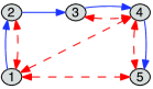
Figure 2: An acyclic mixed graph.

Example 3.

In the graph shown in Figure 2, [(a)]

neither $\pi_{1}\dvtx 2\rightarrow 3\rightarrow 4\leftarrow 3$ nor $\pi_{2}\dvtx 3\rightarrow 4\leftrightarrow 1$ are treks, due to the colliding arrowheads at node $4$.

$\pi\dvtx 2\leftarrow 1\leftrightarrow 4\rightarrow 5$ is a trek, but not a half-trek. $\operatorname{Left}({\pi})=\{1,2\}$ and $\operatorname{Right}({\pi})=\{4,5\}$.

$\pi\dvtx 1\rightarrow 2\rightarrow 3$ is a half-trek with $\operatorname{Left}({\pi})=\{1\}$ and $\operatorname{Right}({\pi})=\{1,2,3\}$.

It will also be important to consider sets of treks. For a set of $n$ treks, $\Pi=\{\pi_{1},\ldots,\pi_{n}\}$, let $x_{i}$ and $y_{i}$ be the source and the target of $\pi_{i}$, respectively. If the sources are all distinct, and the targets are all distinct, then we say that $\Pi$ is a system of treks from $X=\{x_{1},\ldots,x_{n}\}$ to $Y=\{y_{1},\ldots,y_{n}\}$, which we write as $\Pi\dvtx X\rightrightarrows Y$. Note that there may be overlap between the sources in $X$ and the targets in $Y$, that is, we might have $X\cap Y\not=\varnothing$. The system $\Pi$ is a system of half-treks if every trek $\pi_{i}$ is a half-trek. Finally, a set of treks $\Pi=\{\pi_{1},\ldots,\pi_{n}\}$ has no sided intersection if

$$\operatorname{Left}({\pi_{i}})\cap\operatorname{Left}({\pi_{j}})=\varnothing=\operatorname{Right}({\pi_{i}})\cap\operatorname{Right}({\pi_{j}})\qquad\forall i\neq j.$$

Example 4.

Consider again the graph from Figure 2. [(a)]

The pair of treks

$$\pi_{1}\dvtx 3\rightarrow 4\rightarrow 5,\qquad\pi_{2}\dvtx 4\leftrightarrow 1$$

forms a system of treks $\Pi=\{\pi_{1},\pi_{2}\}$ between $X=\{3,4\}$ and $Y=\{1,5\}$. The node $4$ appears in both treks, but is in only the right-hand side of $\pi_{1}$ and only the left-hand side of $\pi_{2}$. Therefore, $\Pi$ has no sided intersection.

The set $\Pi=\{\pi_{1},\pi_{2}\}$ comprising the two treks

$$\pi_{1}\dvtx 1\leftrightarrow 4,\qquad\pi_{2}\dvtx 3\rightarrow 4\rightarrow 5$$

is a system of treks between $X=\{1,3\}$ and $Y=\{4,5\}$. Since node $4$ is in $\operatorname{Right}({\pi_{1}})\cap\operatorname{Right}({\pi_{2}})$, the system $\Pi$ has a sided intersection.

3 Main identifiability and nonidentifiability results

Define the set of parents of a node $v\in V$ as $\mathrm{pa}(v)=\{w\dvtx w\to v\in D\}$ and the set of siblings as $\operatorname{sib}(v)=\{w\dvtx w\leftrightarrow v\in B\}$. Let $\operatorname{htr}(v)$ be the set of nodes in $V\setminus(\{v\}\cup\operatorname{sib}(v))$ that can be reached from $v$ via a half-trek. These half-treks contain at least one directed edge. Put differently, a node $w\not=v$ that is not a sibling of $v$ is in $\operatorname{htr}(v)$ if $w$ is a proper descendant of $v$ or one of its siblings. Here, the term descendant refers to a node that can be reached by a directed path.

Definition 4.

A set of nodes $Y\subset V$ satisfies the half-trek criterion with respect to node $v\in V$ if [(iii)]

$|Y|=|\mathrm{pa}(v)|$,

$Y\cap(\{v\}\cup\operatorname{sib}(v))=\varnothing$, and

there is a system of half-treks with no sided intersection from $Y$ to $\mathrm{pa}(v)$.

We remark that if $\mathrm{pa}(v)=\varnothing$, then $Y=\varnothing$ satisfies the half-trek criterion with respect to $v$. We are now ready to state the main results of this paper.

Theorem 1 ((HTC-identifiability))

Let $(Y_{v}\dvtx v\in V)$ be a family of subsets of the vertex set $V$ of a mixed graph $G$. If, for each node $v$, the set $Y_{v}$ satisfies the half-trek criterion with respect to $v$, and there is a total ordering $\prec$ on the vertex set $V$ such that $w\prec v$ whenever $w\in Y_{v}\cap\operatorname{htr}(v)$, then $G$ is rationally identifiable.

The existence of such a total ordering is equivalent to the relation $w\in Y_{v}\cap\operatorname{htr}(v)$ not admitting cycles; given the family $(Y_{v}\dvtx v\in V)$, this can clearly be tested in polynomial time in the size of the graph. More importantly, as we show in Section 6, HTC-identifiability itself can be checked in polynomial time. In that section we will also show that the same is true for the following nonidentifiability criterion.

Theorem 2 ((HTC-nonidentifiability))

Suppose $G$ is a mixed graph in which every family $(Y_{v}\dvtx v\in V)$ of subsets of the vertex set $V$ either contains a set $Y_{v}$ that fails to satisfy the half-trek criterion with respect to $v$ or contains a pair of sets $(Y_{v},Y_{w})$ with $v\in Y_{w}$ and $w\in Y_{v}$. Then the parametrization $\phi_{G}$ is generically infinite-to-one.

The main ideas underlying the two results are as follows. Under the conditions given in Theorem 1, it is possible to recover the entries in the matrix $\Lambda$, column-by-column, following the given ordering of the nodes. Each column is found by solving a linear equation system that can be proven to have a unique solution. The details of these computations are given in Section 9, where we prove Theorem 1. The proof of Theorem 2 is also in Section 9 and rests on the fact that under the given conditions the Jacobian of $\phi_{G}$ cannot have full rank.

In light of the two theorems, we refer to a mixed graph $G$ as follows: [(iii)]

HTC-identifiable, if it satisfies the conditions of Theorem 1,

HTC-infinite-to-one, if it satisfies the conditions of Theorem 2,

HTC-classifiable, if it is either HTC-identifiable or HTC-infinite-to-one,

HTC-inconclusive, if it is not HTC-classifiable. We now give a first example of an HTC-identifiable graph. Additional examples will be given in Section 5, where we will see graphs that are generically $h$-to-one with $2\leq h<\infty$, but also that HTC-inconclusive graphs may be rationally identifiable or generically infinite-to-one.

Example 5.

The graph in Figure 2 is HTC-identifiable, which can be shown as follows. Let

$$Y_{1}=\varnothing,\qquad Y_{2}=\{5\},\qquad Y_{3}=\{2\},\qquad Y_{4}=\{2\},\qquad Y_{5}=\{3\}.$$

Then each $Y_{v}$ satisfies the half-trek criterion with respect to $v$ because, [(a)]

trivially, $\mathrm{pa}(v)=\varnothing$ for $v=1$;

for $v=2$, we have $5\leftrightarrow 1\rightarrow 2$;

for $v=3$, we have $2\rightarrow 3$;

for $v=4$, we have $2\rightarrow 3\rightarrow 4$; and

for $v=5$, we have $3\rightarrow 4\rightarrow 5$. Considering the descendant sets $\operatorname{htr}(v)$, we find that

$$Y_{1}\cap\operatorname{htr}{(1)} = \varnothing,\qquad Y_{2}\cap\operatorname{htr}{(2)}=\{5\},\qquad Y_{3}\cap\operatorname{htr}{(3)}=\varnothing,$$

$$Y_{4}\cap\operatorname{htr}{(4)} = \{2\},\qquad Y_{5}\cap\operatorname{htr}{(5)}=\{3\}.$$

Hence, any ordering $\prec$ respecting $3\prec 5\prec 2\prec 4$ will satisfy the conditions of Theorem 1.

A mixed graph $G=(V,D,B)$ is simple if there is at most one edge between any pair of nodes, that is, if $D\cap B=\varnothing$ and $v\to w\in D$ implies $w\to v\notin D$. As observed in Brito and Pearl (2002a), simple acyclic mixed graphs are rationally identifiable; compare also Corollary 3 in Drton, Foygel and Sullivant (2011). It is not difficult to see that Theorem 1 includes this observation as a special case.

Proposition 1

If $G$ is a simple acyclic mixed graph, then $G$ is HTC-identifiable.

Since $G$ is simple, it holds for every node $v\in V$ that $\mathrm{pa}(v)\cap\operatorname{sib}(v)=\varnothing$ and, thus, $\mathrm{pa}(v)$ satisfies the half-trek criterion with respect to $v$. An acyclic graph has at least one topological ordering $\prec$, that is, an ordering such that $v\to w\in D$ only if $v\prec w$. In other words, $w\in\mathrm{pa}(v)$ implies $w\prec v$. Hence, the family $(\mathrm{pa}(v)\dvtx v\in V)$ together with a topological ordering $\prec$ satisfies the conditions of Theorem 1.

Another straightforward observation is that the map $\phi_{G}$ cannot be generically finite-to-one if the dimension of the domain of definition $\mathbb{R}^{D}_{\mathrm{reg}}\times\operatorname{PD}(B)$ is larger than the space of $m\times m$ symmetric matrices that contains the image of $\phi_{G}$. This occurs if $|D|+|B|$ is larger than ${{m}\choose{2}}$. Theorem 2 covers this observation.

Proposition 2

If a mixed graph $G=(V,D,B)$ with $V=[m]$ has $|D|+|B|>{{m}\choose{2}}$ edges, then $G$ is HTC-infinite-to-one.

Suppose $G$ is not HTC-infinite-to-one. Then there exists subsets $(Y_{v}\dvtx v\in V)$, where each $Y_{v}$ satisfies the half-trek criterion with respect to $v$ and for any pair of sets $(Y_{v},Y_{w})$ it holds that $v\in Y_{w}$ implies $w\notin Y_{v}$.

Fix a node $v\in V$. For every directed edge $u\to v\in D$, there is a corresponding node $y\in Y_{v}$ for which it holds, by Definition 4, that $y\leftrightarrow v\notin B$. Therefore, if there are $d_{v}$ directed edges pointing to $v$, then there are $d_{v}$ nodes, namely, the ones in $Y_{v}$, that are not adjacent to $v$ in the bidirected part $(V,B)$. If we consider another node $w\in V$, with $d_{w}$ parents, then there are again $d_{w}$ nonadjacencies $\{u,w\}$, $u\in Y_{w}$, in the bidirected part. Moreover, $\{v,w\}$ cannot appear as a nonadjacency for both node $v$ and node $w$ because of the requirement that $v\in Y_{w}$ imply $w\notin Y_{v}$. We conclude that there are at least $|D|$ nonedges in the bidirected part. In other words, $|D|+|B|\leq{{m}\choose{2}}$.

We conclude the discussion of Theorems 1 and 2 by pointing out that HTC-identifiability is equivalent to a seemingly weaker criterion.

Definition 5.

A set of nodes $Y\subset V$ satisfies the weak half-trek criterion with respect to node $v\in V$ if [(iii)]

$|Y|=|\mathrm{pa}(v)|$,

$Y\cap(\{v\}\cup\operatorname{sib}(v))=\varnothing$, and

there is a system of treks with no sided intersection from $Y$ to $\mathrm{pa}(v)$ such that for any $w\in Y\cap\operatorname{htr}(v)$, the trek originating at $w$ is a half-trek.

Lemma 1

Suppose the set $W\subset V$ satisfies the weak half-trek criterion with respect to some node $v$. Then there exists a set $Y$ satisfying the half-trek criterion with respect to $v$, such that $Y\cap\operatorname{htr}(v)=W\cap\operatorname{htr}(v)$.

Lemma 1 yields the following result; both the lemma and the theorem are proved in Section 7 of the supplement [Foygel, Draisma and Drton (2012)].

Theorem 3 ((Weak HTC))

Theorems 1 and 2 hold when using the weak half-trek criterion instead of the half-trek criterion. Moreover, a graph $G$ can be proved to be rationally identifiable (or generically infinite-to-one) using the weak half-trek criterion if and only if $G$ is HTC-identifiable (or HTC-infinite-to-one).

4 G-criterion

The G-criterion, proposed in Brito and Pearl (2006), is a sufficient criterion for rational identifiability in acyclic mixed graphs. The criterion attempts to prove the fiber $\mathcal{F}(\Lambda,\Omega)$ to be equal to $\{(\Lambda,\Omega)\}$ by solving the equation system

$$\Sigma=(I-\Lambda)^{-T}\Omega(I-\Lambda)^{-1}$$

in a stepwise manner. The steps yield the entries in $\Lambda$ column-by-column and, simultaneously, more and more rows and columns for principal submatrices of $\Omega$. As explained in Section 9, the half-trek method from Section 3 starts from an equation system that has $\Omega$ eliminated and then only proves $\Lambda$ to be uniquely identified. In this section, we show that, due to this key simplification, the sufficient condition in the half-trek method improves the G-criterion for acyclic mixed graphs.

To prepare for a comparison of the two criteria, we first restate the identifiability theorem underlying the G-criterion in our own notation. Enumerate the vertex set of an acyclic mixed graph $G$ according to any topological ordering as $V=[m]=\{1,\ldots,m\}$. (Then $v\to w$ only if $v<w$.) Use the ordering to uniquely associate bidirected edges to individual nodes by defining, for each $v\in V$, the sets of siblings $S_{<}(v)=\{w\in\operatorname{sib}(v)\dvtx w<v\}$ and $S_{>}(v)=\{w\in\operatorname{sib}(v)\dvtx w>v\}$. For a trek $\pi$, we write $t(\pi)$ to denote the target node, that is, $\pi$ is a trek from some node to $t(\pi)$.

Definition 6 ([Brito and Pearl (2006)]).

A set of nodes $A\subset V$ satisfies the G-criterion with respect to a node $v\in V$ if $A\subset V\setminus\{v\}$ and $A$ can be partitioned into two (disjoint) sets $Y,Z$ with $|Y|=|\mathrm{pa}(v)|$ and $|Z|=|S_{<}(v)|$, with two systems of treks $\Pi\dvtx Y\rightrightarrows\mathrm{pa}(v)$ and $\Psi\dvtx Z\rightrightarrows S_{<}(v)$, such that the following condition holds:

If each trek $\pi\in\Pi$ is extended to a path $\pi^{\prime}$ by adding the edge $t(\pi)\to v$ to the right-hand side, and each trek $\psi\in\Psi$ is similarly extended using $t(\psi)\leftrightarrow v$, then the set of paths $\{\pi^{\prime}\dvtx\pi\in\Pi\}\cup\{\psi^{\prime}\dvtx\psi\in\Psi\}$ is a set of treks that has no sided intersection except at the common target node $v$.

Note that the paths $\pi^{\prime}$ for $\pi\in\Pi$ are always treks. For $\psi\in\Psi$, the requirement that $\psi^{\prime}$ is a trek means that $\psi$ cannot have an arrowhead at its target node.

For the statement of the main theorem about identifiability using the G-criterion, define the depth of a node $v$ to be the length of the longest directed path terminating at $v$. This number is denoted by $\operatorname{Depth}(v)$.

Theorem 4 ([Brito and Pearl (2006)])

Suppose $(A_{v}\dvtx v\in V)$ is a family of subsets of the vertex set $V$ of an acyclic mixed graph $G$ and, for each $v$, the set $A_{v}$ satisfies the G-criterion with respect to $v$. Then $G$ is rationally identifiable if at least one of the following two conditions is satisfied: [(C1)]

For all $v$ and all $w\in A_{v}$, it holds that $\operatorname{Depth}(w)<\operatorname{Depth}(v)$.

For all $v$ and all $w\in A_{v}\cap(\operatorname{htr}(v)\cup S_{>}(v))$, the trek associated to node $w$ in the definition of the G-criterion is a half-trek. Furthermore, there is a total ordering $\prec$ on $V$, such that if $w\in A_{v}\cap(\operatorname{htr}(v)\cup S_{>}(v))$, then $w\prec v$.

We remark that the ordering $\prec$ in condition (C2) need not agree with any topological ordering of the graph. When using only condition (C1) the theorem was given in Brito and Pearl (2002b), and the literature is not always clear on which version of the G-criterion is concerned. For instance, all examples in Chan and Kuroki (2010) can be proven to be rationally identifiable by means of Theorem 4 as stated here.

We now compare the G-criterion to the half-trek criterion. We say that a graph $G$ is GC-identifiable if it satisfies the conditions of Theorem 4. The next theorem and proposition are proved in Section 4 of the supplement [Foygel, Draisma and Drton (2012)]. They demonstrate that the half-trek method provides an improvement over the G-criterion even for acylic mixed graphs.

Theorem 5

A GC-identifiable acyclic mixed graph is also HTC-identifiable.

The graph in Figure 2 is HTC-identifiable, as was shown in Example 5.

Proposition 3

The acyclic mixed graph in Figure 2 is not GC-identifiable.

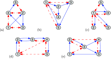
Figure 3: Rationally identifiable mixed graphs.

5 Examples

In the previous section the acyclic mixed graph from Figure 2 was shown to be HTC-identifiable but not GC-identifiable. In this section we give several other examples that illustrate the conditions of our theorems and the ground that lies beyond them. The examples are selected from the computational experiments that we report on in Section 7. We begin with the identifiable class.

Example 6.

Figure 3 shows 5 rationally identifiable mixed graphs: [(a)]

This graph is simple and acyclic and, thus HTC- and GC-identifiable; recall Proposition 1. There are pairs $(\Lambda,\Omega)$ for which the fiber $\mathcal{F}(\Lambda,\Omega)$ has positive dimension. By Theorem 2 in Drton, Foygel and Sullivant (2011), removing the edge $1\leftrightarrow 3$ would give a new graph with all fibers of the form $\mathcal{F}(\Lambda,\Omega)=\{(\Lambda,\Omega)\}$.

The next graph is acyclic but not simple. It is HTC- and GC-identifiable.

This acyclic graph is HTC-inconclusive. The bidirected part being connected, the example is not covered by the graph decomposition technique discussed in Section 8.

This is an example of a cyclic graph that is HTC-identifiable.

This cyclic graph is HTC-inconclusive.

On $m=5$ nodes, graphs with more than ${{5}\choose{2}}=10$ edges are trivially generically infinite-to-one. The next example gives nontrivial nonidentifiable graphs.

Example 7.

All 4 graphs in Figure 4 are generically infinite-to-one. The acyclic graph in (a) and the cyclic graph in (c) are HTC-infinite-to-one. The acyclic graph in (b) and the cyclic graph in (d) are HTC-inconclusive.

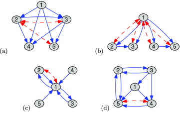
Figure 4: Generically infinite-to-one graphs.

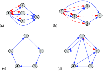
Figure 5: Generically finite-to-one graphs.

Many HTC-inconclusive graphs have fibers that are of cardinality $2\leq h<\infty$. An example of an acyclic 4-node graph that is generically 2-to-one was given in Brito (2004). Our next example lists more graphs of this generically finite-to-one type.

Example 8.

Figure 5 shows four mixed graphs that are HTC-inconclusive and not generically identifiable. All the graphs have fibers that are generically finite: [(a)]

This graph is generically 2-to-1. We note that the coefficients $\lambda_{v5}$, $v\in[4]$, can be identified; that is, any two matrices $\Lambda,\Lambda^{\prime}$ appearing in the same fiber have an identical fifth column.

Generically, the fibers of this graph have cardinality of either one or three. For instance, let

$$\omega_{11}=\cdots=\omega_{55}=1,\qquad\omega_{12}=\omega_{13}=\omega_{15}=\tfrac{1}{5},\qquad\lambda_{23}=1.$$

Define

$$f(\lambda_{12})=529\lambda_{12}^{4}-460\lambda_{12}^{3}-3642\lambda_{12}^{2}-2380\lambda_{12}-4271.$$

Then, not considering the nongeneric situation with $f(\lambda_{12})=0$, we have

$$\bigl{|}\mathcal{F}(\Lambda,\Omega)\bigr{|}=\cases{3,&\quad$\mbox{if }f(\lambda_{12})>0,$\vspace*{2pt}\cr 1,&\quad$\mbox{if }f(\lambda_{12})<0.$}$$

The polynomial $f$ has two roots which are approximately $-2.16$ and $3.44$.

As shown in Drton, Foygel and Sullivant (2011), a cycle of length 3 or more is generically 2-to-1.

The next graph is not generically identifiable. Generically, its fibers have at least two elements but not more than 10. Using the terminology from Definition 7 below, the graph has degree of identifiability 10. We do not know of an example of a fiber with more than two elements.

6 Efficient algorithms for HTC-classification

While purely combinatorial, the identifiability conditions from Theorems 1 and 2 are not in a form that is directly amenable to efficient computation. However, as we show in this section, there exist polynomial-time algorithms for deciding whether a mixed graph $G$ is HTC-identifiable and whether $G$ is HTC-infinite-to-one. In the related context of the G-criterion, Chapter 4 in Brito (2004) describes how the problem of determining the existence of a set of nodes $Y$ satisfying the G-criterion with respect to a given node $v$ can be solved by computation of maximum flow in a derived directed graph. Our work for HTC-identifiability extends this construction, which enables us to use maximum flow computations to completely determine HTC-identifiability of a mixed graph $G$. Furthermore, we show that whether $G$ is HTC-infinite-to-one can be decided via a single max-flow computation.

We first give some background on the max-flow problem; see Ford and Fulkerson (1962) and Cormen et al. (2001). Let $G=(V,D)$ be a directed graph (or “network”) with designated source and sink nodes $s,t\in V$. Let $c_{V}\dvtx V\rightarrow\mathbb{R}_{\geq 0}$ be a node-capacity function, and let $c_{D}\dvtx D\rightarrow\mathbb{R}_{\geq 0}$ be an edge-capacity function. Then a flow $f$ on $G$ is a function $f\dvtx D\rightarrow\mathbb{R}_{\geq 0}$ that satisfies

$$\sum_{u}f(u,v)=\sum_{w}f(v,w)\leq c_{V}(v)$$

for all nodes $v\neq s,t$, and

$$f(u,v)\leq c_{D}(u,v)$$

for all edges $u\rightarrow v\in D$. The size $|f|$ of a flow $f$ on $G$ is the total amount of flow passing from the source $s$ to the sink $t$, that is,

$$|f|:=\sum_{w}f(s,w)=\sum_{u}f(u,t).$$

The max-flow problem on $(G,s,t,c_{V},c_{D})$ is the problem of finding a flow $f$ whose size $|f|$ is maximum.

The computational complexity of the max-flow problem is known to be of order $\mathcal{O}(|V|^{3})$ if $G$ has no reciprocal edge pairs. A reciprocal edge pair consists of the two edges $v\rightarrow w$ and $w\rightarrow v$ for distinct nodes $v\neq w$. (“Antiparallel” is another term used for such edge pairs.) In general, the complexity is $\mathcal{O}((|V|+r)^{3})$, where $r\leq|D|/2$ is the number of reciprocal edge pairs. It is also known that if $c_{V}$ and $c_{D}$ are both integer-valued, then there exists a maximal flow $f$ that is integer-valued, and can be interpreted as a sum of directed paths from $s$ to $t$ with a flow of size $1$ along each path [Ford and Fulkerson (1962), Cormen et al. (2001)]. (We note that the max-flow problem is usually defined without bounded node capacities and on graphs with no reciprocal edge pairs, but the more general problem stated here can be converted to the standard form; see Section 6 of the supplement [Foygel, Draisma and Drton (2012)] for details.)

6.1 Deciding HTC-identifiability

To determine whether a mixed graph $G=(V,D,B)$ is HTC-identifiable, we first need to address the following subproblem. Given a node $v\in V$, and a subset of “allowed” nodes $A\subseteq V\setminus(\{v\}\cup\operatorname{sib}(v))$, how can we efficiently determine whether there exists a subset $Y\subseteq A$ satisfying the half-trek criterion with respect to $v$? We now show that answering this question is equivalent to solving a max-flow problem on a network $G_{\mathrm{flow}}(v,A)$ with at most $2|V|+2$ nodes and at most $3|V|+|D|+|B|$ edges.

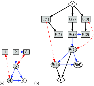
Figure 6: Using max-flow to find a set satisfying the half-trek criterion, for node $v=6$ and allowed nodes $A=\{1,2,3\}$. (a) The concerned mixed graph $G$. (b) The network $G_{\mathrm{flow}}(v,A)$.

We construct the network as follows; an example is shown in Figure 6. The vertex set of $G_{\mathrm{flow}}(v,A)$ comprises three types of nodes, namely, [(a)]

a source $s$ and a sink $t$,

a “left-hand copy” $L(a)$ for each $a\in A$, and

a “right-hand copy” $R(w)$ for each $w\in V$. The edges of $G_{\mathrm{flow}}(v,A)$ are given by the following: [(a)]

$s\rightarrow L(a)$ and $L(a)\rightarrow R(a)$ for each $a\in A$ (thick solid edges, in Figure 6),

$L(a)\rightarrow R(w)$ for each $a\leftrightarrow w\in B$ (dashed edges),

$R(w)\rightarrow R(u)$ for each $w\rightarrow u\in D$ (solid edges), and

$R(w)\rightarrow t$ for each $w\in\mathrm{pa}(v)$ (thick solid edges). Finally, we define the capacity functions. All edges have capacity $\infty$. The source $s$ and sink $t$ have capacity $\infty$, and all other nodes have capacity $1$.

The intuition for our construction is that a half-trek of the form $y\rightarrow x_{1}\rightarrow\cdots\rightarrow x_{n}=p$, with $y\in A$ and $p\in\mathrm{pa}(v)$, will appear in the flow network as

$$s\rightarrow L(y)\rightarrow R(y)\rightarrow R(x_{1})\rightarrow\cdots\rightarrow R(x_{n})\rightarrow t,$$

and a half-trek of the form $y\leftrightarrow x_{1}\rightarrow\cdots\rightarrow x_{n}=p$ will appear as

$$s\rightarrow L(y)\rightarrow R(x_{1})\rightarrow\cdots\rightarrow R(x_{n})\rightarrow t.$$

By construction, no flow can exceed $|\mathrm{pa}(v)|$ in size. Therefore, for practical purposes, all infinite capacities can equivalently be replaced with capacity $|\mathrm{pa}(v)|$.

Algorithm 1 Testing HTC-identifiability of a mixed graph

  Input: $G=(V,D,B)$, a mixed graph on $m$ nodes

  Initialize: $\texttt{SolvedNodes}\leftarrow\{v\dvtx\mathrm{pa}(v)=\varnothing\}$.

  repeat

     for $v=1,2,\ldots,m$ do

        if $v\notin\texttt{SolvedNodes}$ then

           $A\leftarrow(\texttt{SolvedNodes}\cup(V\setminus\operatorname{htr}(v)))\setminus(\{v\}\cup\operatorname{sib}(v))$.

           if $\texttt{MaxFlow}(G_{\mathrm{flow}}(v,A))=|\mathrm{pa}(v)|$ then

              $\texttt{SolvedNodes}\leftarrow\texttt{SolvedNodes}\cup\{v\}$.

           end if

        end if

     end for

  until $\texttt{SolvedNodes}=V$ or no change has occurred in the last iteration.

  Output: “yes” if $\texttt{SolvedNodes}=V$, “no” otherwise.

The following theorem is proved in Section 6 of the supplement.

Theorem 6

Given a mixed graph $G=(V,D,B)$, a node $v\in V$ and a subset of “allowed” nodes $A\subseteq V\setminus(\{v\}\cup\operatorname{sib}(v))$, there exists a set $Y\subseteq A$ satisfying the half-trek criterion with respect to $v$ if and only if the flow network $G_{\mathrm{flow}}(v,A)$ has maximum flow equal to $|\mathrm{pa}(v)|$.

Using Theorem 6, we are able to give an algorithm to determine whether $G$ is HTC-identifiable. If $G$ is HTC-identifiable, then, by Definition 4, we have an ordering $\prec$ on $V$, and for each $v$, a set $Y_{v}$ satisfying the half-trek criterion with respect to $v$, such that any $w\in Y_{v}\cap\operatorname{htr}(v)$ must be $\prec v$. Therefore, by Theorem 6, the network $G_{\mathrm{flow}}(v,A)$ must have maximum flow size $|\mathrm{pa}(v)|$, where $A$ is the set of nodes that are “allowed” to be in $Y_{v}$ according to the ordering $\prec$, that is,

$$A=\bigl{[}\{w\dvtx w\prec v\}\cup\bigl{(}V\setminus\operatorname{htr}(v)\bigr{)}\bigr{]}\setminus\bigl{[}\{v\}\cup\operatorname{sib}(v)\bigr{]}.$$

This intuition is formalized in Algorithm 1. In Section 6 of the supplement, we prove the following theorem, which states that Algorithm 1 correctly determines HTC-identifiability.

Theorem 7

A mixed graph $G=(V,D,B)$ is HTC-identifiable if and only if Algorithm 1 returns “yes.” Furthermore, the algorithm has complexity at most $\mathcal{O}(|V|^{2}(|V|+r)^{3})$, where $r\leq|D|/2$ is the number of reciprocal edge pairs in $D$.

6.2 Deciding if a graph is HTC-infinite-to-one

To determine whether a mixed graph $G=(V,D,B)$ is HTC-infinite-to-one, we may again appeal to max-flow computation. It now suffices to solve a single larger max-flow problem, with at most $\frac{3}{2}|V|^{2}+2$ nodes and at most $|V|\cdot(\frac{3}{2}|V|+2|D|+|B|)$ edges, and $|V|\cdot r$ reciprocal edge pairs, where $r$ is the number of reciprocal edge pairs in $G$.

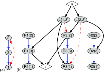
Figure 7: Using max-flow to test whether a mixed graph is HTC-infinite-to-one. (a) A mixed graph $G$ on 3 nodes. (b) The associated flow network $G_{\mathrm{flow}}$.

The relevant flow network $G_{\mathrm{flow}}$ is constructed as follows; an example is shown in Figure 7. The nodes of $G_{\mathrm{flow}}$ are as follows: [(a)]

a source $s$ and a sink $t$,

a “left-hand copy” $L\{v,w\}$ for each unordered pair $\{v,w\}\subset V$ with $v\leftrightarrow w\notin B$, and

a “right-hand copy” $R_{v}(w)$ for each $v,w\in V$. The edges of $G_{\mathrm{flow}}$ are as follows: [(a)]

$s\rightarrow L\{v,w\}$ and $L\{v,w\}\rightarrow R_{v}(w)$ for each unordered pair $\{v,w\}\subset V$ with $v\leftrightarrow w\notin B$ (thick solid edges, in Figure 7),

$L\{v,w\}\rightarrow R_{v}(u)$ for each $v,w,u$ with $v\neq w$ such that $v\leftrightarrow w\notin B$ but $w\leftrightarrow u\in B$ (dashed edges),

$R_{v}(w)\rightarrow R_{v}(u)$ for each $v,w,u\in V$ with $w\rightarrow u\in D$ (solid edges), and

$R_{v}(w)\rightarrow t$ for each $v,w\in V$ with $w\in\mathrm{pa}(v)$ (thick solid edges). Finally, the edge capacity function assigns capacity $\infty$ to all edges, and the node capacity function gives capacity $\infty$ to the source $s$ and sink $t$ and capacity $1$ to all other nodes. If useful in practice, the infinite capacities can be set to $|V|^{2}$, as no flow can have size larger than $|V|^{2}$.

The intuition for the construction just given is as follows. If the mixed graph $G$ is not HTC-infinite-to-one, then simultaneously for all nodes $v\in V$, we can find systems of half-treks with no sided intersection $Y_{v}\rightrightarrows\mathrm{pa}(v)$, such that $Y_{v}$ does not contain $v$ or any siblings of $v$, and $w\in Y_{v}$ implies $v\notin Y_{w}$. Writing $y_{(v,k)}\mbox{$\,\circ$---$\circ\,$}z_{(v,k),1}$ to represent either $y_{(v,k)}=z_{(v,k),1}$ or $y_{(v,k)}\leftrightarrow z_{(v,k),1}$, a half-trek

$$\pi_{(v,k)}\dvtx y_{(v,k)}\mbox{$\,\circ$---$\circ\,$}z_{(v,k),1}\rightarrow z_{(v,k),2}\rightarrow\cdots\rightarrow k$$

with $k\in\mathrm{pa}(v)$ and $y_{(v,k)}\in Y_{v}$ corresponds to a path in the network $G_{\mathrm{flow}}$ given by

$$\tilde{\pi}_{(v,k)}\dvtx s\rightarrow L\{v,y_{(v,k)}\}\rightarrow R_{v}(z_{(v,k),1})\rightarrow R_{v}(z_{(v,k),2})\rightarrow\cdots\rightarrow R_{v}(k)\rightarrow t.$$

Therefore, in the maximum flow on $G_{\mathrm{flow}}$, if $\{v,w\}$ is used by one of the paths passing through the $R_{v}(\cdot)$ copy of the graph, then it will not get used by any of the flows passing through the $R_{w}(\cdot)$ copy of the graph.

The following theorem is proved in Section 6 of the supplement.

Theorem 8

A mixed graph $G=(V,D,B)$ is HTC-infinite-to-one if and only if $G_{\mathrm{flow}}$ has maximum flow size strictly less than $|D|=\sum_{v\in V}|\mathrm{pa}(v)|$. The computational complexity of solving this max-flow problem is$\mathcal{O}(|V|^{3}(|V|+r)^{3})$, where $r\leq|D|/2$ is the number of reciprocal edge pairs in $G$.

7 Computational experiments

This section reports on the results of an exhaustive study of all mixed graphs with $m\leq 5$ nodes, for which the identification problem can be fully solved by means of algebraic techniques. Moreover, we show simulations in which we apply our new combinatorial criteria to graphs with $m=25$ and $50$ nodes.

7.1 Exhaustive computations on small graphs

We applied the half-trek and the G-criterion as well as algebraic techniques to all mixed graphs on $m\leq 5$ nodes. All algebraic computations were done with the software Singular [Decker et al. (2011)]; see Section 1 of the supplement [Foygel, Draisma and Drton (2012)] for details. The G-criterion and the max-flow algorithms from Section 6 were implemented in R [R Development Core Team (2011)] and MATLAB [MathWorks Inc. (2010)], respectively.

Table 1: Classification of unlabeled mixed graphs with $3\leq m\leq 5$ nodes; column “HTC” gives counts of HTC-classifiable graphs

	$\bolds{m=3}$		$\bolds{m=4}$		$\bolds{m=5}$
Unlabeled mixed graphs	Total	HTC	Total	HTC	Total	HTC
Acyclic, $\leq{m\choose 2}$ edges	22		0715		0,103,670
rationally identifiable	17	17	0343	343	00,32,378	032,257
generically finite-to-one	00	–	0004	–	000.,1166	–
generically $\infty$-to-one	05	05	0368	368	00,70,126	070,099
Acyclic, $>{m\choose 2}$ edges	18		0852		0,152,520
Cyclic, $\leq{m\choose 2}$ edges	06		0718		0,348,175
rationally identifiable	02	02	0239	230	00,91,040	078,586
generically finite-to-one	01	–	0075	—	00,44,703	–
generically $\infty$-to-one	03	03	0404	383	0,212,432	202,697
Cyclic, $>{m\choose 2}$ edges	58		9307		8,439,859

The results are given in Table 1, where we treat graphs as unlabeled, that is, we count isomorphism classes of graphs with respect to permutation of the vertex set $V=[m]$. The table distinguishes between acyclic and cyclic (i.e., nonacyclic) graphs. In each case, we single out the graphs with more than ${{m}\choose{2}}$ edges. These are trivially generically infinite-to-one and also HTC-infinite-to-one according to Proposition 2. The remaining graphs are classified into three disjoint groups, namely, rationally identifiable graphs, generically infinite-to-one graphs and generically finite-to-one graphs. The following notion makes the distinctions and terminology precise. Here, $\mathbb{C}^{D}_{\mathrm{reg}}$ is defined as $\mathbb{R}^{D}_{\mathrm{reg}}$ but allowing for complex matrix entries. We write $\mathbb{C}^{m\times m}_{\mathrm{sym}}$ for the space of symmetric $m\times m$ complex matrices.

Definition 7.

Let $G=(V,D,B)$ be a mixed graph. Then the complex rational map $\phi_{G,\mathbb{C}}$, obtained by extending the map $\phi_{G}$ to $\mathbb{C}^{D}_{\mathrm{reg}}\times\mathbb{C}^{m\times m}_{\mathrm{sym}}$, is generically $h$-to-one with $h\in\mathbb{N}\cup\{\infty\}$, and we call $h=\operatorname{ID}(G)$ the degree of identifiability of $G$.

A mixed graph $G$ is rationally identifiable if and only if its degree of identifiability $\operatorname{ID}(G)=1$. Similarly, $G$ is generically infinite-to-one if and only if $\operatorname{ID}(G)=\infty$; in that case the fiber $\mathcal{F}(\Lambda,\Omega)\subset\mathbb{R}^{D}_{\mathrm{reg}}\times\operatorname{PD}(B)$ defined in (4) is generically of positive dimension. In Table 1, a graph $G$ is generically finite-to-one if $2\leq\operatorname{ID}(G)<\infty$ and, thus, $\mathcal{F}(\Lambda,\Omega)$ is generically finite with $|\mathcal{F}(\Lambda,\Omega)|\leq\operatorname{ID}(G)$. If $\operatorname{ID}(G)$ is finite and even, $G$ cannot be generically identifiable because polynomial equations have complex solutions appearing in conjugate pairs and $\mathcal{F}(\Lambda,\Omega)$ always contains at least one (real) point, that is,  $(\Lambda,\Omega)$. If $\operatorname{ID}(G)$ is odd, we cannot exclude the possibility that the equation defining $\mathcal{F}(\Lambda,\Omega)$ generically only has one real point, leading to generic identifiability. However, we did not observe this in any examples we checked.

Table 1 shows that our half-trek method yields a perfect classification of acyclic graphs with $m\leq 4$ nodes and cyclic graphs with $m\leq 3$ nodes. Among the acyclic graphs with $m=5$ nodes, our method misses 121 rationally identifiable graphs and 27 generically infinite-to-one graphs. The gaps are larger for cyclic graphs, but the method still classifies 86% of the rationally identifiable graphs correctly and misses less than 5% of the generically infinite-to-one graphs. In the supplementary article [Foygel, Draisma and Drton (2012)], we list some rationally identifiable graphs and some generically infinite-to-one graphs that are not classifiable using our method (i.e., that are HTC-inconclusive). The degree of identifiability $\operatorname{ID}(G)$ of a graph $G$ with $5$ nodes can be any number in $[8]\cup\{10\}$, and any number in $[4]$ when $G$ is acyclic. For example, the graphs in Figure 5(a), (b) and (d) have $\operatorname{ID}(G)=2$, $3$ and $10$, respectively.

We also tracked which acyclic graphs are rationally identifiable according to the G-criterion from Theorem 4. Since this method depends on the choice of a topological ordering of the nodes, we tested each possible topological ordering. Our computation shows that the G-criterion finds all rationally identifiable acyclic graphs with $m\leq 4$ nodes. For $m=5$, the G-criterion proves 31,830 acyclic graphs to be rationally identifiable but misses 427 of the HTC-identifiable acyclic graphs.

7.2 Simulations for large graphs

Exhaustive computations become prohibitive for more than 5 nodes. Furthermore, algebraic computations are not feasible for larger graphs. Instead, we test the HTC-status of randomly generated mixed graphs with $m=25$ or $m=50$ nodes.

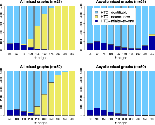
Figure 8: Classification of labeled mixed graphs with $m=25$ and $m=50$ nodes. Each bar represents 5000 randomly drawn graphs with fixed number of edges, ranging from $m$ to $m\cdot 10$.

For each value $n=k\cdot m$ for $k\in[10]$, we randomly sampled $5000$ labeled mixed graphs on $m$ nodes with $n$ edges, by selecting a subset of size $n$ from the set of all possible edges, which consists of $2\cdot{{m}\choose{2}}$ directed edges and ${m\choose 2}$ bidirected edges. We repeated this process with acyclic graphs only; the choice is then from ${m\choose 2}$ directed edges and ${m\choose 2}$ bidirected edges. The results of these simulations are shown in Figure 8. When the graphs are restricted to be acyclic, most are HTC-identifiable and only extremely few are HTC-inconclusive. When we do not restrict to acyclic graphs, on the other hand, we see that as the number of edges increases, the proportion of HTC-inconclusive graphs grows rapidly.

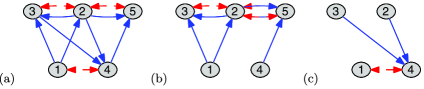
Figure 9: An acyclic mixed graph shown in (a) and its two mixed components shown in (b) and (c).

8 Decomposition of acyclic graphs

In this section we discuss how, for acyclic graphs, the scope of applicability of our half-trek method can be extended via a graph decomposition due to Tian (2005). Let $G=(V,D,B)$ be an acyclic mixed graph, and let $C_{1},\ldots,C_{k}\subset V$ be the (pairwise disjoint) vertex sets of the connected components of the bidirected part $(V,B)$. For $j\in[k]$, let $B_{j}=B\cap(C_{j}\times C_{j})$ be the bidirected edges in the $j$th connected component. Let $V_{j}$ be the union of $C_{j}$ and any parents of nodes in $C_{j}$, that is,

$$V_{j}=C_{j}\cup\bigl{\{}\mathrm{pa}(v)\dvtx v\in C_{j}\bigr{\}},\qquad j=1,\ldots,k.$$

Clearly, the sets $V_{1},\ldots,V_{k}$ need not be pairwise disjoint. Let $D_{j}$ be the set of edges $v\to w$ in the directed part $(V,D)$ that have $v\in V_{j}$ and $w\in C_{j}$. The decomposition of Tian (2005) involves the graphs $G_{j}=(V_{j},D_{j},B_{j})$, for $j\in[k]$. We refer to these as the mixed components $G_{1},\ldots,G_{k}$ of $G$. Figure 9 gives an example.

The mixed components $G_{1},\ldots,G_{k}$ create a partition of the edges of $G$. There is an associated partition of the entries of $\Lambda\in\mathbb{R}^{D}$ that yields submatrices $\Lambda_{1},\ldots,\Lambda_{k}$ with each $\Lambda_{j}\in\mathbb{R}^{D_{j}}$; recall that for an acyclic graph $\mathbb{R}^{D}_{\mathrm{reg}}=\mathbb{R}^{D}$. Similarly, from $\Omega\in\operatorname{PD}(B)$, we create matrices $\Omega_{1},\ldots,\Omega_{k}$ with each $\Omega_{j}\in\operatorname{PD}(B_{j})$, where $\operatorname{PD}(B_{j})$ is defined with respect to the graph $G_{j}$, that is, the set contains matrices indexed by $V_{j}\times V_{j}$. We define $\Omega_{j}$ by taking the submatrix $\Omega_{C_{j},C_{j}}$ from $\Omega$ and extending it by setting $(\Omega_{j})_{vv}=1$ for all $v\in V_{j}\setminus C_{j}$. The work leading up to Theorems 1 and 2 in Tian (2005) shows that, for all $j\in[k]$, there is a rational map $f_{j}$ defined on the entire cone of $m\times m$ positive definite matrices such that

$$f_{j}\circ\phi_{G}(\Lambda,\Omega)=\phi_{G_{j}}(\Lambda_{j},\Omega_{j})$$

for all $\Lambda\in\mathbb{R}^{D}$ and $\Omega\in\operatorname{PD}(B)$. In turn, there is a rational map $g$ defined everywhere on the product of the relevant cones of positive definite matrices such that

$$g\bigl{(}\phi_{G_{1}}(\Lambda_{1},\Omega_{1}),\ldots,\phi_{G_{k}}(\Lambda_{k},\Omega_{k})\bigr{)}=\phi_{G}(\Lambda,\Omega)$$

for all $\Lambda\in\mathbb{R}^{D}$ and $\Omega\in\operatorname{PD}(B)$. We thus obtain the following theorem.

Theorem 9

For an acyclic mixed graph $G$ with mixed components $G_{1},\ldots,G_{k}$, the following holds: [(iii)]

$G$ is rationally (or generically) identifiable if and only if all components $G_{1},\ldots,G_{k}$ are rationally (or generically) identifiable;

$G$ is generically infinite-to-one if and only if there exists a component $G_{j}$ that is generically infinite-to-one;

if each $G_{j}$ is generically $h_{j}$-to-one with $h_{j}<\infty$, then $G$ is generically $h$-to-one with $h=\prod_{j=1}^{k}h_{j}$.

We remark that this theorem could also be stated as $\operatorname{ID}(G)=\prod_{j=1}^{k}\operatorname{ID}(G_{j})$, in terms of the degree of identifiability from Definition 7.

The next theorem makes the observation that when applying our half-trek method to an acyclic graph, we may always first decompose the graph into its mixed components, which may result into computational savings.

Theorem 10

If an acyclic mixed graph $G$ is HTC-identifiable, then all its mixed components $G_{1},\ldots,G_{k}$ are HTC-identifiable. Furthermore, $G$ is HTC-infinite-to-one if and only if there exists a mixed component $G_{j}$ that is HTC-infinite-to-one.

The claim about HTC-identifiability follows from Lemma 4 in Section 5 of the supplement [Foygel, Draisma and Drton (2012)]. The second statement is a consequence of Lemmas 5 and 6 from the same section.

The benefit of graph decomposition goes beyond computation in that some identification methods apply to all mixed components but not to the original graph. In Tian (2005), this is exemplified for the G-criterion. More precisely, the 4-node example given there concerns the early version of the G-criterion from Brito and Pearl (2002b) that includes only condition (C1) from Theorem 4 but not condition (C2), which is due to Brito and Pearl (2006). However, graph decomposition allows one to also extend the scope of our more general half-trek method, where passing to mixed components can avoid problems with finding a suitable total ordering of the vertex set. Surprisingly, however, the extension is possible only for the sufficient condition, that is, HTC-identifiability; Theorem 10 gives an equivalence result for HTC-infinite-to-one graphs.

Proposition 4

The acyclic mixed graph in Figure 9(a) is not HTC-identifiable but both its mixed components are HTC-identifiable.

Suppose for a contradiction that the original graph $G$ is HTC-identifiable and that the sets $Y_{3}$, $Y_{4}$ and $Y_{5}$ are part of the family of sets appearing in Theorem 1. In particular, each set has two elements and satisfies the half-trek criterion with respect to its subscript. Now, the presence of the edge $2\leftrightarrow 3$ implies that $Y_{3}\subset\{1,4,5\}$. Moreover, $Y_{3}\not=\{1,4\}$ because the sole half-trek from $4$ to $3$ has $1$ in its right-hand side and all half-treks from $1$ to $3$ are directed paths and thus have the source $1$ on their right-hand side as well. It follows that $5\in Y_{3}$ and, thus, $3\notin Y_{5}$. Since $2\leftrightarrow 5$ is in $G$, it must hold that $Y_{5}=\{1,4\}$. Examining the descendant sets $\operatorname{htr}(v)$, we see that the total ordering $\prec$ in Theorem 1 ought to satisfy $4\prec 5\prec 3$. Since $1\in\operatorname{sib}(4)$ and $3,5\in\operatorname{htr}(4)$, we conclude that $Y_{4}\subset\{2\}$, which is a contradiction because $Y_{4}$ must have two elements.

Turning to the mixed components of $G$, it is clear that the component shown in Figure 9(c) is HTC-identifiable because it is a simple graph; recall Proposition 1. The component in Figure 9(b) is HTC-identifiable because Theorem 1 applies with the choice of

$$Y_{1}=Y_{4}=\varnothing,\qquad Y_{2}=\{1\},\qquad Y_{5}=\{1,4\},\qquad Y_{3}=\{1,5\},$$

and any ordering that respects $5\prec 3$.

As seen in Table 1, the half-trek method misses 121 rationally identifiable acyclic graphs with 5 nodes, among them is the example from Proposition 4. After graph decomposition, the half-trek method proves 9 of the 121 examples to be rationally identifiable. The remaining 112 graphs all have a connected bidirected part; see Figure 3(c) for an example. On 5 nodes, there are 27 generically infinite-to-one graphs that are HTC-inconclusive. All of these have a connected bidirected part.

9 Proofs for the half-trek criterion

In this section we prove the two main theorems stated in Section 3. We begin with the identifiability theorem.

Theorem 1 ((HTC-identifiability))

Let $(Y_{v}\dvtx v\in V)$ be a family of subsets of the vertex set $V$ of a mixed graph $G$. If, for each node $v$, the set $Y_{v}$ satisfies the half-trek criterion with respect to $v$, and there is a total ordering $\prec$ on the vertex set $V$ such that $w\prec v$ whenever $w\in Y_{v}\cap\operatorname{htr}(v)$, then $G$ is rationally identifiable.

Let $\Sigma=\phi_{G}(\Lambda_{0},\Omega_{0})$ be a matrix in the image of $\phi_{G}$, given by a generically chosen pair $(\Lambda_{0},\Omega_{0})\in\Theta=\mathbb{R}^{D}_{\mathrm{reg}}\times\operatorname{PD}(B)$. For generic identifiability, we need to show that the equation

$$\Sigma=(I-\Lambda)^{-T}\Omega(I-\Lambda)^{-1}$$ (9)

has a unique solution in $\Theta$, namely, $(\Lambda,\Omega)=(\Lambda_{0},\Omega_{0})$. However, a pair $(\Lambda,\Omega)$ solves (9) if and only if

$$\bigl{[}(I-\Lambda)^{T}\Sigma(I-\Lambda)\bigr{]}_{vw}=0\qquad\forall(v,w)\notin B\mbox{ and }v\not=w$$ (10)

and

$$\bigl{[}(I-\Lambda)^{T}\Sigma(I-\Lambda)\bigr{]}_{vw}=\Omega_{vw}\qquad\forall(v,w)\in B\mbox{ or }v=w.$$ (11)

The nonzero entries of $\Omega$ appearing in (11) are freely varying real numbers that are subject only to the requirement that $\Omega$ be positive definite. For cyclic graphs, (9) contains rational equations. Hence, the focus is on (10), which defines a polynomial equation system even when the graph is cyclic.

We prove the theorem by solving the equations (10) in a stepwise manner according to the ordering $\prec$. When visiting node $v$, the goal is to recover the $v$th column of $\Lambda$ as a function of $\Sigma$. Based on solving linear equation systems, the functions of $\Sigma$ that give the entries of $\Lambda$ will always be rational functions, proving our stronger claim of rational (as opposed to mere generic) identifiability.

For our proof we proceed by induction and assume that, for all $w\prec v$, we have recovered the entries of the vector $\Lambda_{\mathrm{pa}(w),w}$ as (rational) expressions in $\Sigma$. To solve for $\Lambda_{\mathrm{pa}(v),v}$, let $Y_{v}=\{y_{1},\ldots,y_{n}\}$ and $\mathrm{pa}(v)=\{p_{1},\ldots,p_{n}\}$. Define $\mathbf{A}\in\mathbb{R}^{n\times n}$ as

$$\mathbf{A}_{ij}=\cases{\bigl{[}(I-\Lambda)^{T}\Sigma\bigr{]}_{y_{i}p_{j}},&\quad$\mbox{if }y_{i}\in\operatorname{htr}(v),$\vspace*{2pt}\cr\Sigma_{y_{i}p_{j}},&\quad$\mbox{if }y_{i}\notin\operatorname{htr}(v).$}$$

Define $\mathbf{b}\in\mathbb{R}^{n}$ as

$$\mathbf{b}_{i}=\cases{\bigl{[}(I-\Lambda)^{T}\Sigma\bigr{]}_{y_{i}v},&\quad${\mbox{if }y_{i}\in\operatorname{htr}(v),}$\vspace*{2pt}\cr\Sigma_{y_{i}v},&\quad${\mbox{if }y_{i}\notin\operatorname{htr}(v).}$}$$

Note that both $\mathbf{A}$ and $\mathbf{b}$ depend only on $\Sigma$ and the columns $\Lambda_{\mathrm{pa}(w),w}$ with $w\in Y_{v}\cap\operatorname{htr}(v)$, which are assumed already to be known as a function of $\Sigma$ because $w\in Y_{v}\cap\operatorname{htr}(v)$ implies $w\prec v$. We now claim that the vector $\Lambda_{\mathrm{pa}(v),v}$ solves the equation system $\mathbf{A}\cdot\Lambda_{\mathrm{pa}(v),v}=\mathbf{b}$.

First, consider an index $i$ with $y_{i}\in Y_{v}\cap\operatorname{htr}(v)$. Since $Y_{v}$ satisfies the half-trek criterion with respect to $v$, the node $y_{i}\not=v$ is not a sibling of $v$. Therefore, by (10),

$$\bigl{[}(I-\Lambda)^{T}\ \Sigma(I-\Lambda)\bigr{]}_{y_{i}v}=0\quad\Longrightarrow\qquad\bigl{[}(I-\Lambda)^{T}\Sigma\Lambda\bigr{]}_{y_{i}v}=\bigl{[}(I-\Lambda)^{T}\Sigma\bigr{]}_{y_{i}v}.$$

It follows that

$$(\mathbf{A}\cdot\Lambda_{\mathrm{pa}(v),v})_{i} = \sum_{j=1}^{n}\bigl{[}(I-\Lambda)^{T}\Sigma)\bigr{]}_{y_{i}p_{j}}\Lambda_{p_{j}v}$$

$$= \bigl{[}(I-\Lambda)^{T}\Sigma\Lambda\bigr{]}_{y_{i}v}=\bigl{[}(I-\Lambda)^{T}\Sigma\bigr{]}_{y_{i}v}=\mathbf{b}_{i}.$$

Second, let $i$ be an index with $y_{i}\in Y_{v}\setminus\operatorname{htr}(v)$. Then

$$(\mathbf{A}\cdot\Lambda_{\mathrm{pa}(v),v})_{i}=\sum_{j=1}^{n}\Sigma_{y_{i}p_{j}}\Lambda_{p_{j}v}=[\Sigma\Lambda]_{y_{i}v}=\bigl{[}(I-\Lambda)^{-T}\Omega(I-\Lambda)^{-1}\Lambda\bigr{]}_{y_{i}v}.$$

By definition of $\operatorname{htr}(v)$, we know that $[(I-\Lambda)^{-T}\Omega]_{y_{i}v}=0$. Adding this zero and using that $(I-\Lambda)^{-1}=I+(I-\Lambda)^{-1}\Lambda$, we obtain that

$$(\mathbf{A}\cdot\Lambda_{\mathrm{pa}(v),v})_{i} = \bigl{[}(I-\Lambda)^{-T}\Omega(I-\Lambda)^{-1}\Lambda\bigr{]}_{y_{i}v}+\bigl{[}(I-\Lambda)^{-T}\Omega\bigr{]}_{y_{i}v}$$

$$= \bigl{[}(I-\Lambda)^{-T}\Omega(I-\Lambda)^{-1}\bigr{]}_{y_{i}v}=\Sigma_{y_{i}v}=\mathbf{b}_{i}.$$

Therefore, $\mathbf{A}\cdot\Lambda_{\mathrm{pa}(v),v}=\mathbf{b}$, as claimed.

By Lemma 2 below, the matrix $\mathbf{A}$ is invertible in the generic situation. Therefore, we have shown that $\Lambda_{\mathrm{pa}(v),v}=\mathbf{A}^{-1}\mathbf{b}$ is a rational function of $\Sigma$. Proceeding inductively according to the vertex ordering $\prec$, we recover $\Lambda_{\mathrm{pa}(v),v}$ for all $v$ and, thus, the entire matrix $\Lambda$, as desired.

Lemma 2

Let $v\in V$ be any node. Let $Y\subset V\setminus(\{v\}\cup\operatorname{sib}(v))$, with $|Y|=|\mathrm{pa}(v)|=n$. Write $Y=\{y_{1},\ldots,y_{n}\}$ and $\mathrm{pa}(v)=\{p_{1},\ldots,p_{n}\}$, and define the matrix $\mathbf{A}$ as

$$\mathbf{A}_{ij}=\cases{\bigl{[}(I-\Lambda)^{T}\Sigma\bigr{]}_{y_{i}p_{j}},&\quad$y_{i}\in\operatorname{htr}(v),$\vspace*{2pt}\cr\Sigma_{y_{i}p_{j}},&\quad$y_{i}\notin\operatorname{htr}(v).$}$$

If $Y$ satisfies the half-trek criterion with respect to $v$, then $\mathbf{A}$ is generically invertible.

Recall the trek-rule from (8). Let $\mathcal{H}(v,w)\subset\mathcal{T}(v,w)$ be the set of all half-treks from $v$ to $w$. Then, for each $i,j\in\{1,\ldots,n\}$,

$$\mathbf{A}_{ij}=\cases{\displaystyle\sum_{\pi\in\mathcal{H}(y_{i},p_{j})}\pi(\lambda,\omega),&\quad$y_{i}\in\operatorname{htr}(v),$\vspace*{2pt}\cr\displaystyle\sum_{\pi\in\mathcal{T}(y_{i},p_{j})}\pi(\lambda,\omega),&\quad$y_{i}\notin\operatorname{htr}(v).$}$$

For a system of treks $\Pi$, define the monomial

$$\Pi(\lambda,\omega)=\prod_{\pi\in\Pi}\pi(\lambda,\omega).$$

Then

$$\operatorname{det}(\mathbf{A})=\sum_{\Psi\dvtx Y\rightrightarrows P}(-1)^{|\Psi|}\Psi(\lambda,\omega),$$

where the sum is over systems of treks $\Psi$ for which all treks $\psi\in\Psi$ with sources in $\operatorname{htr}(v)$ are half-treks. (The sign $|\Psi|$ is the sign of the permutation that writes $p_{1},\ldots,p_{n}$ in the order of their appearance as targets of the treks in $\Psi$.)

By assumption, there exists some system of half-treks with no sided intersection from $Y$ to $P$. Let $\Pi$ be such a system, with minimal total length among all such systems. Now take any system of treks $\Psi$ from $Y$ to $P$, such that $\Pi(\lambda,\omega)=\Psi(\lambda,\omega)$. (We do not assume that $\Psi$ has no sided intersection, or has any half-treks.) In Lemma 1 in the supplement [Foygel, Draisma and Drton (2012)], we prove that $\Psi=\Pi$ for any such $\Psi$—that is, $\Pi$ is the unique system of half-treks with no sided intersection of minimal total length. Therefore, the coefficient of the monomial $\Pi(\lambda,\omega)$ in $\operatorname{det}(\mathbf{A})$ is given by $(-1)^{|\Pi|}$, and $\operatorname{det}(\mathbf{A})$ is not the zero polynomial/power series. For generic choices of $(\Lambda,\Omega)$ it thus holds that $\operatorname{det}(\mathbf{A})\not=0$.

We now turn to the proof of the nonidentifiability theorem.

Theorem 2 ((HTC-nonidentifiability))

Suppose $G$ is a mixed graph in which every family $(Y_{v}\dvtx v\in V)$ of subsets of the vertex set $V$ either contains a set $Y_{v}$ that fails to satisfy the half-trek criterion with respect to $v$ or contains a pair of sets $(Y_{v},Y_{w})$ with $v\in Y_{w}$ and $w\in Y_{v}$. Then the parametrization $\phi_{G}$ is generically infinite-to-one.

Let

$$N=\bigl{\{}\{v,w\}\dvtx v\neq w,(v,w)\notin B\bigr{\}}$$

be the set of (unordered) nonsibling pairs in the graph. Treating $\Sigma$ as fixed, let $\mathbf{J}\in\mathbb{R}^{|N|\times|D|}$ be the Jacobian of the equations in (10), taking partial derivatives with respect to the nonzero entries of $\Lambda$. The entries of $\mathbf{J}$ are given by

$$\mathbf{J}_{\{v,w\},(u,v)}=-\bigl{[}(I-\Lambda)^{T}\Sigma\bigr{]}_{wu},\qquad\{v,w\}\in N,u\in\mathrm{pa}(v),$$ (12)

and all other entries zero. By Lemma 2 in the supplement, it is sufficient to show that, under the conditions of the theorem, $\mathbf{J}$ does not have generically full column rank.

In the remainder of this proof, we always let $\Sigma=\phi_{G}(\Lambda,\Omega)$ when considering $\mathbf{J}$. If $\mathbf{J}$ has generically full column rank, then we can choose a set $M\subset N$ with $|M|=|D|=\sum_{v\in V}|\mathrm{pa}(v)|$, such that $\operatorname{det}(\mathbf{J}_{M,D})$ is not the zero polynomial, where $\mathbf{J}_{M,D}$ is the square submatrix formed by taking all rows of $\mathbf{J}$ that are indexed by $M$. By the definition of the determinant, there must be a partition of $M=\bigcup_{v}M_{v}$ such that for all $v$, we have

$$\operatorname{det}(\mathbf{J}_{M_{v},(\mathrm{pa}(v),v)})\neq 0.$$

By (12), each entry $\{w_{1},w_{2}\}\in M_{v}$ must have either $w_{1}=v$ or $w_{2}=v$. Writing $Y_{v}=\{w\dvtx\{v,w\}\in M_{v}\}$, it holds that

$$\operatorname{det}\bigl{(}\bigl{[}(I-\Lambda)^{T}\Sigma\bigr{]}_{Y_{v},\mathrm{pa}(v)}\bigr{)}=\pm\operatorname{det}(J_{\{Y_{v},v\},(\mathrm{pa}(v),v)})=\pm\operatorname{det}(J_{M_{v},(\mathrm{pa}(v),v)})$$

is nonzero. By Lemma 3 below, this implies that each set $Y_{v}$ satisfies the half-trek criterion with respect to its indexing node $v$. Forming a partition of $M\subset N$, the sets $M_{v}$ are pairwise disjoint. Hence, no two nodes $v,w$ can satisfy both $v\in Y_{w}$ and $w\in Y_{v}$ because otherwise $\{v,w\}\in M_{v}\cap M_{w}$.

Lemma 3

Let $v\in V$ be any node. Let $Y\subset V\setminus(\{v\}\cup\operatorname{sib}(v))$, with $|Y|=|\mathrm{pa}(v)|=n$. If the matrix $\mathbf{J}=[(I-\Lambda)^{T}\Sigma]_{Y,\mathrm{pa}(v)}$ is generically invertible, then $Y$ satisfies the half-trek criterion with respect to $v$.

Abbreviate $P=\mathrm{pa}(v)$. We have $\mathbf{J}=[(I-\Lambda)^{T}\Sigma]_{Y,P}=[\Omega(I-\Lambda)^{-1}]_{Y,P}$. Hence,

$$\operatorname{det}(\mathbf{J})=\sum_{W\subset V,|W|=n}\operatorname{det}(\Omega_{Y,W})\operatorname{det}\bigl{(}(I-\Lambda)^{-1}_{W,P}\bigr{)}.$$

By assumption, $\operatorname{det}(\mathbf{J})$ is not the zero polynomial/power series. Therefore, for some $W\subset V$ with $|W|=n$, we have $\operatorname{det}(\Omega_{Y,W})\not\equiv 0$ and $\operatorname{det}((I-\Lambda)^{-1}_{W,P})\not\equiv 0$.

By Menger’s theorem [see, e.g., Theorem 9.1 of Schrijver (2004)], the nonvanishing of $\operatorname{det}((I-\Lambda)^{-1}_{W,P})$ implies that there is a system $\Psi$ of pairwise vertex-disjoint directed paths $\psi_{i}\dvtx w_{i}\rightarrow\cdots\rightarrow p_{i}$, $i\in[n]$, whose sources and targets give $W=\{w_{1},\ldots,w_{n}\}$ and $P=\{p_{1},\ldots,p_{n}\}$, respectively. Indeed, if no such system exists, then by Menger’s theorem there is a set $C$ of strictly less than $n$ vertices such that all directed paths from $W$ to $P$ pass through $C$. But this implies that the matrix $(I-\Lambda)^{-1}_{W,P}$ factors as $(I-\Lambda)^{-1}_{W,C}\cdot(I-\Lambda)^{-1}_{C,P}$, and $|C|<n$ implies that $\operatorname{det}((I-\Lambda)^{-1}_{W,P})=0$, a contradiction. Note that by erasing loops, we can further arrange that the $\psi_{i}$ do not have self-intersections.

Since $\operatorname{det}(\Omega_{Y,W})\neq 0$, we can index $Y=\{y_{1},\ldots,y_{n}\}$ such that $\Omega_{y_{i}w_{i}}\neq 0$ for all $i$. This implies that either $y_{i}=w_{i}$ or $y_{i}\leftrightarrow w_{i}\in B$. Now define a system of half-treks $\Pi\dvtx Y\rightrightarrows P$ by setting $\pi_{i}=\psi_{i}$ if $w_{i}=y_{i}$, and extending $\psi_{i}$ at the left-hand side to

$$\pi_{i}=y_{i}\leftrightarrow w_{i}\rightarrow\cdots\rightarrow p_{i}$$

if $y_{i}\neq w_{i}$. Since $\Psi$ has no sided intersection, $\Pi$ also has no sided intersection. It follows that $Y$ satisfies the half-trek criterion with respect to $v$.

10 Conclusion

We have proposed graphical criteria for determining identifiability as well as nonidentifiability of linear structural equation models. The criteria can be checked in time that is polynomial in the size of the mixed graph representing the model. To our knowledge, they are the best known. In particular, they apply to cyclic graphs. For acyclic graphs, the graph decomposition method discussed in Section 8 further extends their scope. We expect the decomposition method to also extend the scope of the criteria for cyclic graphs, when a cyclic model is suitably embedded into an acyclic one, but we leave a thorough study of this problem for future work.

Our algebraic computations revealed that there remains a “gap” between the necessary and the sufficient condition for rational identifiability that we have developed. To better understand this gap, it would be helpful to find an interesting class of graphs, defined on an arbitrary number of nodes $m$, which is rationally identifiable but not HTC-identifiable.

In models that are not HTC-identifiable, the half-trek method can still prove certain parameters to be rationally identifiable; recall, for instance, the example from Figure 5(a). Referring to Theorem 1, if a set $Y_{v}$ satisfies the half-trek criterion with respect to the indexing node $v$, and $Y_{v}\cap\operatorname{htr}(v)=\varnothing$, then the proof of Theorem 1 shows how to obtain rational expressions in the covariance matrix $\Sigma$ that equal the coefficients $\lambda_{wv}$, where $w\in\mathrm{pa}(v)$. In the next step of the recursive procedure that proves Theorem 1, we can solve for any node $u$ with $Y_{u}\cap\operatorname{htr}(u)\subseteq\{v\}$. Continuing in this way, individual parameters can be identified even though ultimately the procedure will stop before all nodes are visited, as we are discussing an HTC-inconclusive graph. In particular, the maximum flow construction given in Algorithm 1 will reveal all nodes whose set of incoming directed edge parameters can be identified via the half-trek criterion. It would be interesting to compare this partial application of the half-trek method to other graphical criteria for identification of individual edge coefficients; see, in particular, Garcia-Puente, Spielvogel and Sullivant (2010) for a review and examples of such methods.

References

- Bollen (1989) {bbook}[mr] \bauthor\bsnmBollen, \bfnmKenneth A.\binitsK. A. (\byear1989). \btitleStructural Equations with Latent Variables. \bpublisherWiley, \baddressNew York. \bidmr=0996025 \bptokimsref \endbibitem
- Brito (2004) {bmisc}[author] \bauthor\bsnmBrito, \bfnmCarlos\binitsC. (\byear2004). \bhowpublishedGraphical methods for identification in structural equation models. Ph.D. thesis, UCLA Computer Science Dept. \bptokimsref \endbibitem
- Brito and Pearl (2002a) {barticle}[mr] \bauthor\bsnmBrito, \bfnmCarlos\binitsC. and \bauthor\bsnmPearl, \bfnmJudea\binitsJ. (\byear2002a). \btitleA new identification condition for recursive models with correlated errors. \bjournalStruct. Equ. Model. \bvolume9 \bpages459–474. \biddoi=10.1207/S15328007SEM0904_1, issn=1070-5511, mr=1930449 \bptokimsref \endbibitem
- Brito and Pearl (2002b) {binproceedings}[author] \bauthor\bsnmBrito, \bfnmCarlos\binitsC. and \bauthor\bsnmPearl, \bfnmJudea\binitsJ. (\byear2002b). \btitleA graphical criterion for the identification of causal effects in linear models. In \bbooktitleProceedings of the Eighteenth National Conference on Artificial Intelligence (AAAI) \bpages533–538. \bpublisherAAAI press, \baddressPalo Alto, CA. \bptokimsref \endbibitem
- Brito and Pearl (2006) {binproceedings}[author] \bauthor\bsnmBrito, \bfnmCarlos\binitsC. and \bauthor\bsnmPearl, \bfnmJudea\binitsJ. (\byear2006). \btitleGraphical condition for identification in recursive SEM. In \bbooktitleProceedings of the Twenty-Second Conference on Uncertainty in Artificial Intelligence (\beditor\bfnmRina\binitsR. \bsnmDechter and \beditor\bfnmThomas S.\binitsT. S. \bsnmRichardson, eds.) \bpages47–54. \bpublisherAUAI Press, \baddressArlington, VA. \bptokimsref \endbibitem
- Chan and Kuroki (2010) {binproceedings}[author] \bauthor\bsnmChan, \bfnmHei\binitsH. and \bauthor\bsnmKuroki, \bfnmManabu\binitsM. (\byear2010). \btitleUsing descendants as instrumental variables for the identification of direct causal effects in linear SEMs. In \bbooktitleProceedings of the Thirteenth International Conference on Artificial Intelligence and Statistics (\beditor\bfnmYee Whye\binitsY. W. \bsnmTeh and \beditor\bfnmMike\binitsM. \bsnmTitterington, eds.). \bseriesJ. Mach. Learn. Res. (JMLR), Workshop and Conference Proceedings \bvolume9 \bpages73–80. \bnoteAvailable at http://jmlr.csail.mit.edu/proceedings/. \bptokimsref \endbibitem
- Cormen et al. (2001) {bbook}[mr] \bauthor\bsnmCormen, \bfnmThomas H.\binitsT. H., \bauthor\bsnmLeiserson, \bfnmCharles E.\binitsC. E., \bauthor\bsnmRivest, \bfnmRonald L.\binitsR. L. and \bauthor\bsnmStein, \bfnmClifford\binitsC. (\byear2001). \btitleIntroduction to Algorithms, \bedition2nd ed. \bpublisherMIT Press, \baddressCambridge, MA. \bidmr=1848805 \bptokimsref \endbibitem
- Cox, Little and O’Shea (2007) {bbook}[mr] \bauthor\bsnmCox, \bfnmDavid\binitsD., \bauthor\bsnmLittle, \bfnmJohn\binitsJ. and \bauthor\bsnmO’Shea, \bfnmDonal\binitsD. (\byear2007). \btitleIdeals, Varieties, and Algorithms, \bedition3rd ed. \bpublisherSpringer, \baddressNew York. \biddoi=10.1007/978-0-387-35651-8, mr=2290010 \bptokimsref \endbibitem
- Decker et al. (2011) {bmisc}[author] \bauthor\bsnmDecker, \bfnmWolfram\binitsW., \bauthor\bsnmGreuel, \bfnmGert-Martin\binitsG.-M., \bauthor\bsnmPfister, \bfnmGerhard\binitsG. and \bauthor\bsnmSchönemann, \bfnmHans\binitsH. (\byear2011). \bhowpublishedSingular 3-1-3—A computer algebra system for polynomial computations. Available at http:// www.singular.uni-kl.de. \bptokimsref \endbibitem
- Didelez, Meng and Sheehan (2010) {barticle}[mr] \bauthor\bsnmDidelez, \bfnmVanessa\binitsV., \bauthor\bsnmMeng, \bfnmSha\binitsS. and \bauthor\bsnmSheehan, \bfnmNuala A.\binitsN. A. (\byear2010). \btitleAssumptions of IV methods for observational epidemiology. \bjournalStatist. Sci. \bvolume25 \bpages22–40. \biddoi=10.1214/09-STS316, issn=0883-4237, mr=2741813 \bptokimsref \endbibitem
- Drton, Foygel and Sullivant (2011) {barticle}[mr] \bauthor\bsnmDrton, \bfnmMathias\binitsM., \bauthor\bsnmFoygel, \bfnmRina\binitsR. and \bauthor\bsnmSullivant, \bfnmSeth\binitsS. (\byear2011). \btitleGlobal identifiability of linear structural equation models. \bjournalAnn. Statist. \bvolume39 \bpages865–886. \biddoi=10.1214/10-AOS859, issn=0090-5364, mr=2816341 \bptokimsref \endbibitem
- Evans and Ringel (1999) {barticle}[author] \bauthor\bsnmEvans, \bfnmWilliam N.\binitsW. N. and \bauthor\bsnmRingel, \bfnmJeanne S.\binitsJ. S. (\byear1999). \btitleCan higher cigarette taxes improve birth outcomes? \bjournalJournal of Public Economics \bvolume72 \bpages135–154. \bptokimsref \endbibitem
- Ford and Fulkerson (1962) {bbook}[mr] \bauthor\bsnmFord, \bfnmL. R.\binitsL. R. \bsuffixJr. and \bauthor\bsnmFulkerson, \bfnmD. R.\binitsD. R. (\byear1962). \btitleFlows in Networks. \bpublisherPrinceton Univ. Press, \baddressPrinceton, NJ. \bidmr=0159700 \bptokimsref \endbibitem
- Foygel, Draisma and Drton (2012) {bmisc}[author] \bauthor\bsnmFoygel, \bfnmRina\binitsR., \bauthor\bsnmDraisma, \bfnmJan\binitsJ. and \bauthor\bsnmDrton, \bfnmMathias\binitsM. (\byear2012). \bhowpublishedSupplement to “Half-trek criterion for generic identifiability of linear structural equation models.” DOI:\doiurl110.1214/12-AOS1012SUPP. \bptokimsref \endbibitem
- Garcia-Puente, Spielvogel and Sullivant (2010) {binproceedings}[author] \bauthor\bsnmGarcia-Puente, \bfnmLuis D.\binitsL. D., \bauthor\bsnmSpielvogel, \bfnmSarah\binitsS. and \bauthor\bsnmSullivant, \bfnmSeth\binitsS. (\byear2010). \btitleIdentifying causal effects with computer algebra. In \bbooktitleProceedings of the Twenty-sixth Conference on Uncertainty in Artificial Intelligence (UAI) (\beditor\bfnmPeter\binitsP. \bsnmGrünwald and \beditor\bfnmPeter\binitsP. \bsnmSpirtes, eds.). \bpublisherAUAI Press. \bptokimsref \endbibitem
- MathWorks Inc. (2010) {bmisc}[author] \borganizationMathWorks Inc. (\byear2010). \bhowpublishedMATLAB version 7.10.0 (R2010a). Natick, MA. \bptokimsref \endbibitem
- Okamoto (1973) {barticle}[mr] \bauthor\bsnmOkamoto, \bfnmMasashi\binitsM. (\byear1973). \btitleDistinctness of the eigenvalues of a quadratic form in a multivariate sample. \bjournalAnn. Statist. \bvolume1 \bpages763–765. \bidissn=0090-5364, mr=0331643 \bptokimsref \endbibitem
- Pearl (2000) {bbook}[mr] \bauthor\bsnmPearl, \bfnmJudea\binitsJ. (\byear2000). \btitleCausality: Models, Reasoning, and Inference. \bpublisherCambridge Univ. Press, \baddressCambridge. \bidmr=1744773 \bptokimsref \endbibitem
- R Development Core Team (2011) {bmisc}[author] \borganizationR Development Core Team. (\byear2011). \bhowpublishedR: A language and environment for statistical computing. R Foundation for Statistical Computing, Vienna, Austria. \bptokimsref \endbibitem
- Richardson and Spirtes (2002) {barticle}[mr] \bauthor\bsnmRichardson, \bfnmThomas\binitsT. and \bauthor\bsnmSpirtes, \bfnmPeter\binitsP. (\byear2002). \btitleAncestral graph Markov models. \bjournalAnn. Statist. \bvolume30 \bpages962–1030. \biddoi=10.1214/aos/1031689015, issn=0090-5364, mr=1926166 \bptokimsref \endbibitem
- Schrijver (2004) {bbook}[author] \bauthor\bsnmSchrijver, \bfnmAlexander\binitsA. (\byear2004). \btitleCombinatorial Optimization. Polyhedra and Efficiency. \bseriesAlgorithms and Combinatorics 24 \bvolumeA. \bpublisherSpringer, \baddressBerlin. \bptokimsref \endbibitem
- Spirtes, Glymour and Scheines (2000) {bbook}[mr] \bauthor\bsnmSpirtes, \bfnmPeter\binitsP., \bauthor\bsnmGlymour, \bfnmClark\binitsC. and \bauthor\bsnmScheines, \bfnmRichard\binitsR. (\byear2000). \btitleCausation, Prediction, and Search, \bedition2nd ed. \bpublisherMIT Press, \baddressCambridge, MA. \bidmr=1815675 \bptokimsref \endbibitem
- Sullivant, Talaska and Draisma (2010) {barticle}[mr] \bauthor\bsnmSullivant, \bfnmSeth\binitsS., \bauthor\bsnmTalaska, \bfnmKelli\binitsK. and \bauthor\bsnmDraisma, \bfnmJan\binitsJ. (\byear2010). \btitleTrek separation for Gaussian graphical models. \bjournalAnn. Statist. \bvolume38 \bpages1665–1685. \biddoi=10.1214/09-AOS760, issn=0090-5364, mr=2662356 \bptokimsref \endbibitem
- Tian (2005) {binproceedings}[author] \bauthor\bsnmTian, \bfnmJin\binitsJ. (\byear2005). \btitleIdentifying direct causal effects in linear models. In \bbooktitleProceedings of the Twentieth National Conference on Artificial Intelligence (AAAI) \bpages346–353. \bpublisherAAAI press, \baddressPalo Alto, CA. \bptokimsref \endbibitem
- Tian (2009) {binproceedings}[author] \bauthor\bsnmTian, \bfnmJin\binitsJ. (\byear2009). \btitleParameter identification in a class of linear structural equation models. In \bbooktitleProceedings of the Twenty-first International Joint Conference on Artificial Intelligence (IJCAI) \bpages1970–1975. \bpublisherAAAI press, \baddressPalo Alto, CA. \bptokimsref \endbibitem
- Wermuth (2011) {barticle}[mr] \bauthor\bsnmWermuth, \bfnmNanny\binitsN. (\byear2011). \btitleProbability distributions with summary graph structure. \bjournalBernoulli \bvolume17 \bpages845–879. \biddoi=10.3150/10-BEJ309, issn=1350-7265, mr=2817608 \bptokimsref \endbibitem
- Wright (1921) {barticle}[author] \bauthor\bsnmWright, \bfnmSewall\binitsS. (\byear1921). \btitleCorrelation and causation. \bjournalJ. Agricultural Research \bvolume20 \bpages557–585. \bptokimsref \endbibitem
- Wright (1934) {barticle}[author] \bauthor\bsnmWright, \bfnmSewall\binitsS. (\byear1934). \btitleThe method of path coefficients. \bjournalAnn. Math. Statist. \bvolume5 \bpages161–215. \bptokimsref \endbibitem