Efficient Instance Retrieval of Subgoals
for Subsumptive Tabled Evaluation
of Logic Programs

Abstract

Tabled evaluation is an implementation technique that solves some problems of traditional Prolog systems in dealing with recursion and redundant computations. Most tabling engines determine if a tabled subgoal will produce or consume answers by using variant checks. A more refined method, named call subsumption, considers that a subgoal $A$ will consume from a subgoal $B$ if $A$ is subsumed by (an instance of) $B$, thus allowing greater answer reuse. We recently developed an extension, called Retroactive Call Subsumption, that improves upon call subsumption by supporting bidirectional sharing of answers between subsumed/subsuming subgoals. In this paper, we present both an algorithm and an extension to the table space data structures to efficiently implement instance retrieval of subgoals for subsumptive tabled evaluation of logic programs. Experiments results using the YapTab tabling system show that our implementation performs quite well on some complex benchmarks and is robust enough to handle a large number of subgoals without performance degradation.

1 Introduction

Tabled resolution methods solve some of the shortcomings of Prolog because they can reduce the search space, avoid looping and have better termination properties than SLD resolution methods [Chen and Warren (1996)]. Tabling works by memorizing generated answers and then by reusing them on similar calls that appear during the resolution process. In a nutshell, first calls to tabled subgoals are considered generators and are evaluated as usual, using SLD resolution, but their answers are stored in a global data space, called the table space. Similar calls are called consumers and are resolved by consuming the answers already stored for the corresponding generator, instead of re-evaluating them against the program clauses. There are two main approaches to determine if two subgoals $A$ and $B$ are similar:

• Variant-based tabling: $A$ and $B$ are variants if they can be made identical by variable renaming. For example, $p(X,1,Y)$ and $p(Y,1,Z)$ are variants because both can be transformed into $p(VAR_{0},1,VAR_{1})$;

• Subsumption-based tabling: $A$ is considered similar to $B$ if $A$ is subsumed by $B$ (or $B$ subsumes $A$), i.e., if $A$ is more specific than $B$ (or an instance of). For example, subgoal $p(X,1,2)$ is subsumed by subgoal $p(Y,1,Z)$ because there is a substitution $\{Y=X,Z=2\}$ that makes $p(X,1,2)$ an instance of $p(Y,1,Z)$. Tabling by call subsumption is based on the principle that if $A$ is subsumed by $B$ and $S_{A}$ and $S_{B}$ are the respective answer sets, then $S_{A}\subseteq S_{B}$. Note that this assumption may not hold when programs use extra-logical features of Prolog such as the var/1 and nonvar/1 built-in predicates.

For some types of programs, subsumption-based tabling yields superior time performance, as it allows greater reuse of answers, and better space usage, since the answer sets for the subsumed subgoals are not stored. However, the mechanisms to efficiently support subsumption-based tabling are harder to implement, which makes subsumption-based tabling not as popular as variant-based tabling. XSB Prolog [Rao et al. (1997)] was the first Prolog system to implement subsumption-based tabling, first by using a data structure called Dynamic Threaded Sequential Automata (DTSA) [Rao et al. (1996)] and later by using a data structure called Time-Stamped Trie (TST) [Johnson et al. (1999), Johnson (2000)], that showed better space efficiency than DTSA. Despite the advantages of using subsumption-based tabling, the degree of answer reuse might depend on the call order of subgoals. For example, in XSB, if a more general subgoal is called before specific subgoals, answer reuse will happen, but if more specific subgoals are called before a more general subgoal, no reuse will occur.

In order to solve this problem, we implemented an extension to the original TST design, called Retroactive Call Subsumption (RCS) [Cruz and Rocha (2010)], that supports subsumption-based tabling by allowing full sharing of answers between subsumptive subgoals, independently of the order they are called. RCS works by selectively pruning the evaluation of subsumed subgoals when a more general subgoal appears later on. We designed a new table space organization, called Single Time-Stamped Trie (STST) [Cruz and Rocha (2010)] where answers are represented only once. We also designed a new algorithm to efficiently retrieve the set of currently evaluating subgoals that are subsumed by (instances of) a more general subgoal. In this paper, we will focus our discussion on the support for this algorithm on a concrete implementation, the YapTab system [Rocha et al. (2005), Rocha et al. (2000)], but our proposals can be generalized and applied to other tabling systems based on similar data structures.

The remainder of the paper is organized as follows. First, we briefly introduce the main background concepts about the table space in YapTab. Next, we describe the modifications made to the table space data structures and we discuss in detail our new algorithm to efficiently retrieve subsumed subgoals. Finally, we present some experimental results and then we finish by outlining some conclusions.

2 Table Space

Whenever a tabled subgoal is first called, a new entry is allocated in the table space. Table entries are used to keep track of subgoal calls and to store their answers. Arguably, the most successful data structure for tabling is tries [Ramakrishnan et al. (1999)]. Tries are trees in which common prefixes are represented only once. Tries provide complete discrimination for terms and permit look-up and insertion to be done in a single pass. Figure 1 shows an example of a trie. First, in (a) the trie is only represented by a root node. Next, in (b) the term $t(X,a)$ is inserted and three nodes are created to represent each part of the term. In (c) a new term, $u(X,b,Y)$ is inserted. This new term differs from the first one and a new distinct branch is created. Finally, in (d), the term $t(1,a)$ is inserted and only one new node needs to be created as this term shares the two prefix nodes with term $t(X,a)$. Note that $t(1,a)$ is subsumed by $t(X,a)$ since there is a substitution, namely $\{X=1\}$, that makes $t(1,a)$ an instance of $t(X,a)$.

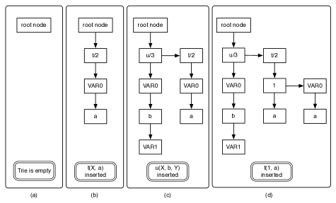
Figure 1: Using tries to represent terms

In YapTab, we use the trie node data structure as the building block of tries. Each node contains the following fields: $symbol$, representing the stored part of a term; $child$, a pointer to the child node; $parent$, a pointer to the parent node; $sibling$, which points to the sibling node; and $status$, a bit field with information about the trie node. When the chain of sibling nodes exceeds a certain threshold length, a hashing scheme is dynamically employed to provide direct access to nodes, optimizing the search of terms.

In the STST organization, each tabled predicate has a table entry that points to a subgoal trie and an answer trie. In the subgoal trie, each distinct trie path represents a tabled subgoal call and each leaf trie node points to a subgoal frame, a data structure containing information about the subgoal call, notably an answer return list containing pointers to leaf nodes of the answer trie. In order to support call subsumption mechanisms, the answer trie is also a time-stamped trie [Johnson et al. (1999)], where the trie nodes are extended with a $timestamp$ field.

3 Retrieval of Subsumed Subgoals

In this section, we describe the modifications made to the subgoal trie data structure and we discuss in detail the new algorithm developed to efficiently retrieve the set of currently evaluating instances of a subgoal. Note that in a RCS setting, this new algorithm is executed only when the currently executing subgoal is a generator (and not a consumer of answers) and a call represents a generator only if no variant or subsuming subgoals are found during an initial search on the subgoal trie. This initial search is done in a single pass through the subgoal trie using the method initially proposed by [Rao et al. (1996)] for non-retroactive subsumption-based tabling.

3.1 Subgoal Trie Data Structure

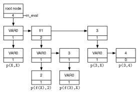
Figure 2: The $in\_eval$ field in a subgoal trie representing a $p/2$ tabled predicate

Each subgoal trie node was extended with a new field, named $in\_eval$, which stores the number of subgoals, represented below the node, that are in evaluation. During the search for subsumed subgoals, this field is used to ignore the subgoal trie branches without evaluating subgoals, i.e., the ones with $in\_eval=0$.

When a subgoal starts being evaluated, all subgoal trie nodes in its subgoal trie path get the $in\_eval$ field incremented. When a subgoal completes its evaluation, the corresponding $in\_eval$ fields are decremented. Hence, for each subgoal leaf trie node, the $in\_eval$ field can be equal to either: 1, when the corresponding subgoal is in evaluation; or 0, when the subgoal is completed. For the root subgoal trie node, we know that it will always contain the total number of subgoals being currently evaluated. For an example, the subgoal trie in Fig. 2 represents four evaluating subgoals and one completed subgoal for the tabled predicate $p/2$.

When a chain of sibling nodes is organized in a linked list, it is easy to select the trie branches with evaluating subgoals by looking for the nodes with $in\_eval>0$. But, when the sibling nodes are organized in a hash table, it can become very slow to inspect each node as the number of siblings increase. In order to solve this problem, we designed a new data structure, called evaluation index, in a similar manner to the timestamp index [Johnson et al. (1999)] of the TST design.

An evaluation index is a double linked list that is built for each hash table and is used to chain the subgoal trie nodes where the $in\_eval$ field is greater than 0. Note that this linked list is not ordered by the $in\_eval$ value. Each evaluation index node contains the following fields: $prev$, a pointer to the previous evaluation index node, if any; $next$, a pointer to the next evaluation index node, if any; $node$, a pointer to the subgoal trie node the index node represents; and $in\_eval$, the number of evaluating subgoals under the corresponding subgoal trie node. We also extended the hash table with a field named $index$ to point to the evaluation index.

An indexed subgoal trie node uses the $in\_eval$ field to point to the index node, while a trie node with $in\_eval=0$ is not indexed. To compute the $in\_eval$ value of a trie node, we first need to use the $status$ field to determine if the node is inside a hash table or not, and then use the $in\_eval$ field accordingly. Figure 3 shows a hash table and the corresponding evaluation index.

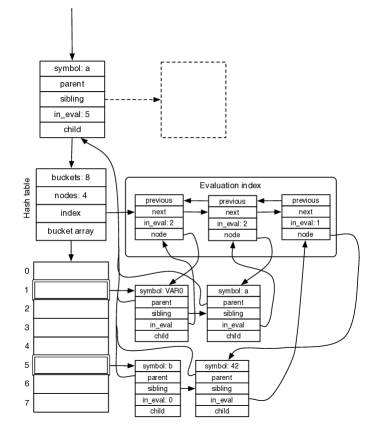
Figure 3: A hash table with an evaluation index

The evaluation index makes the operation of pruning trie branches more efficient by providing direct access to trie nodes with evaluating subgoals, instead of visiting a potentially large number of trie nodes in the hash table. While advantageous, the operation of incrementing or decrementing the $in\_eval$ fields in a trie path is more costly, because these indexes must be maintained.

Figure 4 presents the pseudo-code for the $increment\_in\_eval()$ procedure. This procedure iterates over the subgoal trie path and increments the $in\_eval$ field from the leaf to the root node. When we find hashed trie nodes, we must check if the node is currently being indexed. If this is the case, we simply increment the $in\_eval$ field of the index node, otherwise we create a new index node on the evaluation index pointing to the current subgoal trie node and the $in\_eval$ field of the subgoal trie node is made to point to the index node.

increment_in_eval(leaf_node, root_node) {
  current_node = leaf_node
  while (current_node != root_node)
    if (is_hashed_node(current_node))
      if (in_eval(current_node) == 0)                         // not indexed
        hash_table = child(parent(current_node))
        index_node = add_index_node(hash_table, current_node)
        in_eval(current_node) = index_node
      else                                                        // indexed
        index_node = in_eval(current_node)
        in_eval(index_node) = in_eval(index_node) + 1
    else                                                // simple chain list
      in_eval(current_node) = in_eval(current_node) + 1
    current_node = parent(current_node)
  in_eval(root_node) = in_eval(root_node) + 1
}

Figure 4: Pseudo-code for procedure $increment\_in\_eval()$

The procedure in Fig. 5, $decrement\_in\_eval()$, does the inverse job of procedure $increment\_in\_eval()$. When decrementing an indexed subgoal trie node, if the $in\_eval$ field reaches 0, the trie node no longer needs to be indexed, and hence we must remove the index node from the evaluation index. In the other cases, we simply decrement the respective $in\_eval$ field.

decrement_in_eval(leaf_node, root_node) {
  current_node = leaf_node
  while (current_node != root_node)
    if (is_hashed_node(current_node))
      index_node = in_eval(current_node)
      if (in_eval(index_node) == 1)                     // remove from index
        hash_table = child(parent(current_node))
        remove_index_node(hash_table, index_node)
        in_eval(current_node) = 0
      else                                                   // keep indexed
        in_eval(index_node) = in_eval(index_node) - 1
    else                                                // simple chain list
      in_eval(current_node) = in_eval(current_node) - 1
    current_node = parent(current_node)
  in_eval(root_node) = in_eval(root_node) - 1
}

Figure 5: Pseudo-code for procedure $decrement\_in\_eval()$

3.2 Matching Algorithm

The algorithm that finds the currently running subgoals that are subsumed by a more general subgoal $S$ works by matching the subgoal arguments $SA$ of $S$ against the trie symbols in the subgoal trie $T$. By using the $in\_eval$ field as described previously, we can ignore irrelevant branches as we descend the trie. When reaching a leaf node, we append the corresponding subgoal frame in a result list that is returned once the process finishes. If the matching process fails at some point or if a leaf node was reached, the algorithm backtracks to try alternative branches, in order to fully explore the subgoal trie $T$.

When traversing $T$, trie variables cannot be successfully matched against ground terms of $SA$. Ground terms of $SA$ can only be matched with ground terms of $T$. For example, if matching the trie subgoal $p(VAR_{0},VAR_{1})$ with the subgoal $p(2,X)$, we cannot match the constant $2$ against the trie variable $VAR_{0}$, because $p(2,X)$ does not subsume $p(X,Y)$.

When a variable of $SA$ is matched against a ground term of $T$, subsequent occurrences of the same variable must also match the same term. As an example, consider the trie subgoal $p(2,4)$ and the subgoal $p(X,X)$. The variable $X$ is first matched against 2, but the second matching, against 4, must fail because $X$ is already bound to 2.

Now consider the trie subgoal $p(VAR_{0},VAR_{1})$ and the subgoal $p(X,X)$. Variable $X$ is first matched against $VAR_{0}$, but then we have a second match against a different trie variable, $VAR_{1}$. Again, the process must fail because $p(X,X)$ does not subsume $p(X,Y)$. This last example evokes a new rule for variable matching. When a variable of $SA$ is matched against a trie variable, subsequent occurrences of the same variable must always match the same trie variable. This is necessary, because the subgoals found must be instances of $S$. To implement this algorithm, we use the following data structures:

• WAM data structures: heap, trail, and associated registers. The heap is used to build structured terms, in which the subgoal arguments are bound. Whenever a new variable is bound, we trail it using the WAM trail;

• term stack: stores the remaining terms to be matched against the subgoal trie symbols;

• term log stack: stores already matched terms from the term stack and is used to restore the state of the term stack when backtracking;

• variable enumerator vector: used to mark the term variables that were matched against trie variables;

• choice point stack: stores choice point frames, where each frame contains information needed to restore the computation in order to search for alternative branches.

Figure 6 shows the pseudo-code for the procedure that traverses a subgoal trie and collects the set of subsumed subgoals of a given subgoal call. This procedure can be summarized in the following steps:

1. setup WAM machinery and define the current trie node as the trie root node;

2. push the subgoal arguments into the term stack from right to left, so that the leftmost argument is on the top;

3. fetch a term $T$ from the term stack;

4. search for a child trie node $N$ of the current node where the $in\_eval$ field is not 0.

5. search for the next child node with a valid $in\_eval$ field to be pushed on the choice point stack, if any;

6. match $T$ against the trie symbol of $N$;

7. proceed into the child of $N$ or, if steps 4 or 6 fail, backtrack by popping a frame from the choice point stack. The frame is used to restore the term stack from the term log stack and to set the current trie node to the alternative node;

8. once a leaf is reached, add the corresponding subgoal frame to the resulting subgoal frame list. If there are choice points available, backtrack to try them;

9. if no more choice point frames exist, return the found subsumed subgoals.

collect_subsumed_subgoals(subgoal_trie, subgoal_call) {
  save_wam_registers()
  subgoals = NULL
  parent = subgoal_trie
  node = child(parent)
  push_arguments(term_stack, subgoal_call)
  while (true)
    term = deref(pop(term_stack))
    if (is_atom(term) or is_integer(term))
      try_node = try_constant_term(term, node)
    else if (is_functor(term) or is_list(term))
      try_node = try_structured_term(term, node)
    else                                          // term must be a variable
      try_node = try_variable_term(term, node)
    if (try_node != NULL)
      push(term_log_stack, term)
      parent = try_node
      node = child(parent)
      if (empty(term_stack))                   // new subsumed subgoal found
        add_subgoal(subgoals, subgoal_frame(parent))
      else
        continue
    if (empty(choice_point_stack))
      unwind_wam_trail()
      restore_wam_registers()
      return subgoals
    else
      frame = pop_choice_point_frame(choice_point_stack)
      restore_computation(frame)
      node = get_alt_node(frame)
      parent = parent(node)
}

Figure 6: Pseudo-code for procedure $collect\_subsumed\_subgoals()$

3.3 Choice Point Stack

To store alternative branches for exploration, we use a choice point stack. Each choice point frame stores the following fields: $alt\_node$, the alternative node to explore; $term\_stack\_top$, the top of the term stack; $term\_log\_stack\_top$, the top of the term log stack; $trail\_top$, the current trail position; and $saved\_HB$, the $HB$ register. The $HB$ register is used to detect conditional bindings in the same manner as for the $HB$ register in WAM choice points, that is, we use it to know if a term variable needs to be trailed. When a choice point frame is popped from the stack, the state of the computation is restored by executing the following actions:

• all terms stored in the term log stack are pushed back to the term stack in the inverse order (topmost terms are pushed first);

• the trail is unwound to reset the variables that were bound after choice point creation;

• register $H$ and $HB$ are reset to their previous values. $H$ is set to $HB$ and $HB$ to $saved\_HB$;

• the current node and parent node are reset.

Since constant and structured terms can have at most one matching alternative in a trie level, choice point frames are only pushed when the current term is a variable. Remember that if a node satisfies the $in\_eval$ prerequisite, variable terms can match all types of trie symbols, including trie variables.

3.4 Matching Constant and Structured Terms

If the next term from the term stack is a constant or a structured term we must match it against a similar ground term only. Both constant and structured terms work pretty much the same way, except that for a list or a functor term we push the term arguments into the term stack before descending into the next trie level. The arguments are pushed into the stack in order to be matched against the next trie symbols. Figure 7 presents the pseudo-code for the $try\_structured\_term()$ procedure.

try_structured_term(term, current_node)
  if (is_hash_table(current_node))              // step 1: check hash bucket
    hash_table = current_node
    current_node = search_bucket_array(hash_table, term)
    if (current_node == NULL)
      return NULL
  while (current_node != NULL)    // step 2: traverse chain of sibling nodes
    if (symbol(current_node) == principal_functor(term))
      if (in_eval(current_node) > 0)
        push_arguments(term_stack, term)
        return current_node
      else                                      // no running subgoals below
        return NULL
    current_node = sibling(current_node)
  return NULL
}

Figure 7: Pseudo-code for procedure $try\_structured\_term()$

This procedure is divided into two steps. In step 1, we check if the current node is a hash table. If this is the case, we hash the term to get the hash bucket that might contain the matching trie node. If the bucket is empty we simply return $NULL$. Otherwise, we move into step 2. In step 2 we traverse a chain of sibling nodes (a simple chain or a bucket chain) looking for a node with a matching symbol and with a valid $in\_eval$ value.

3.5 Matching Variable Terms

A variable term can potentially be matched against any trie symbol. It is only when the variable is matched against a trie variable that the process may fail. Figure 8 shows the pseudo-code for the $try\_variable\_term()$ procedure. It is defined by three main cases, depending on the type of the current node, namely:

1. the node is a hash table. For faster access of valid trie nodes, we use the evaluation index, which gives us all the valid trie nodes in a linked list. We set the next alternative node to be pushed on the choice point stack by using the function $next\_valid\_index\_node()$ that uses the $next$ pointer of the first index node to locate the alternative trie node.

2. the node is a hashed node, thus is on the evaluation index of the corresponding hash table. In this case, we also use the $next\_valid\_index\_node()$ function to identify the next alternative trie node.

3. the node is part of a simple linked list. Here we must use the function $next\_valid\_node()$ to find the next valid trie node ($in\_eval>0$). The alternative trie node is also set using this function on the sibling node.

try_variable_term(variable, current_node) {
  if (is_hash_table(current_node))                     // case 1: hash table
    hash_table = current_node
    index_node = index(hash_table)
    if (index_node == NULL)                     // no running subgoals below
      return NULL
    current_node = node(index_node)
    alt_node = next_valid_index_node(current_node)
  else if (is_hashed_node(current_node))             // case 2: indexed node
    alt_node = next_valid_index_node(current_node)
  else                                         // case 3: simple linked list
    current_node = next_valid_node(current_node)
    if (current_node == NULL)
      return NULL
    alt_node = next_valid_node(current_node)
  push_choice_point_frame(choice_point_stack, {alt_node, ..., HB})
  if (try_variable_matching(variable, symbol(current_node)))
    return current_node
  else
    return NULL
}

Figure 8: Pseudo-code for procedure $try\_variable\_term()$

After the current valid node and alternative node are set, we push the alternative into the choice point stack and call the $try\_variable\_matching()$ procedure (Fig. 9) to match the term variable with the trie node symbol.

try_variable_matching(variable, symbol) {
  if (is_variable(symbol))
    if (is_in_variable_enumerator_vector(variable))
      return (variable_enumerator_index(variable) == var_index(symbol))
    else                                               // free term variable
      var_index = var_index(symbol)
      mark_variable_enumerator_vector(variable, var_index)
      return TRUE
  else                                                 // ground trie symbol
    if (is_in_variable_enumerator_vector(variable))
      return FALSE
    if (is_constant(symbol))
      bind_and_conditionally_trail(variable, symbol)
    else if (is_functor(symbol) or is_list(symbol))
      term = create_heap_structure(symbol)
      bind_and_conditionally_trail(variable, term)
      push_arguments(term_stack, term)
    return TRUE
}

Figure 9: Pseudo-code for procedure $try\_variable\_matching()$

Matching a term variable with a trie symbol depends on the type of the trie symbol. If the trie symbol is a trie variable, we have two cases. If the term variable is free (i.e., this is its first occurrence), we simply make it to point to the position on the variable enumerator vector that corresponds to the trie variable index and we trail the term variable using the WAM trail. Otherwise, the term variable is already matched against a trie variable (on the variable enumerator vector), thus we get both indexes (term and trie variable indexes) and the matching succeeds if they correspond to the same index (same variable).

If the trie symbol is a ground term, we first test if the term variable is on the variable enumerator vector and, in such case, we fail since term variables matched against trie variables must only be matched against the same trie variable. For constant trie symbols, we simply bind the term variable to the trie symbol. For structured terms (lists and functors), we create the structured term on the heap, bind the term variable to the heap address, and push the new term arguments into the term stack to be matched against the next trie symbols.

3.6 Running Example

Consider the subgoal trie in Fig. 10 representing three evaluating subgoals and two completed subgoals for a tabled predicate $p/3$. Now assume that we want to retrieve the subgoals that are subsumed by the subgoal call $p(X,2,X)$.

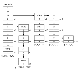
Figure 10: A subgoal trie for a $p/3$ tabled predicate with three evaluating subgoals

Initially, the algorithm sets up the WAM registers and then pushes the subgoal arguments into the term stack, resulting in the following stack configuration (from bottom to top): $[X,2,X]$. Next, we pop the $X$ variable from the term stack and inspect the linked list of nodes $n1$, $n9$ and $n12$. Because $X$ is a variable term, we can potentially match this term with any node with $in\_eval>0$. We thus match $X$ against the trie symbol $f/1$ from node $n1$ by constructing a new $f/1$ functor term into the heap and by binding $X$ to it (this includes trailing $X$’s reference). Figure 11(a) shows the configuration of the auxiliary data structures at this point. Notice that the $H$ register now points to the next free heap cell, the $X$ variable ($REF~{}7$) was pushed into the term log stack, and the new variable representing the argument of $f/1$ ($REF~{}12$) was pushed into the term stack. Before descending into node $n2$, we need to push the alternative node $n12$ into the choice point stack. Note that node $n9$ cannot be used as an alternative because no evaluating subgoals exist in that trie branch.

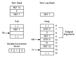
(a) Before descending into node $n2$

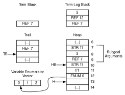
(b) After descending into node $n7$

Figure 11: Auxiliary data structures configuration

Next, we pop the unbound functor argument from the term stack and we match it against the trie symbol 3 from node $n2$. Node $n5$ is then pushed into the choice point stack, and we now have the following choice point stack configuration: $[n12,n5]$. We then descend into node $n3$, where the next term from the term stack, 2, matches the trie symbol 2. Here, there are no alternative nodes to explore, and matching proceeds to node $n4$. In node $n4$, we first pop the $X$ variable from the term stack that, after dereferenced, points to the constructed $f/1$ functor on the heap. As we cannot match ground terms with trie variables, the process fails.

We then pop the top frame from the choice point stack and search is resumed at node $n5$. The resulting choice point stack configuration is $[n12]$. Because we backtracked to try node $n5$, the term stack is restored with the $X$ variable ($REF~{}7$), the constant 2 and the functor argument ($REF~{}12$). In node $n5$, the functor argument is popped from the term stack and, because the trie symbol is the $VAR_{0}$ trie variable, it is made to point to the index 0 of the variable enumerator vector. We then descend into node $n6$, where matching succeeds and then we arrive at node $n7$. Figure 11(b) shows the configuration of the auxiliary data structures at this point. Notice that the twelfth cell on the heap now points to a variable enumerator position and that the $HB$ register points again to the tenth cell on the heap, which corresponds to the value of the $H$ register when we pushed the choice point frame for the alternative node $n12$.

Node $n7$ contains the functor $f/1$ and the next term from the term stack is the $X$ variable ($REF~{}7$) that is bound to the functor $f/1$ created on the heap. Matching therefore succeeds and we get into node $n8$. In node $n8$, we have the trie variable $VAR_{0}$ and a variable that is in the variable enumerator vector. Because they both correspond to the same index, index 0, matching succeeds and a first subsumed subgoal is found: $p(f(X),2,f(X))$.

Next, we pop the next top frame from the choice point stack and search is resumed at node $n12$. The term stack is restored to its initial state and the choice point stack is now empty. Node $n12$ contains the trie symbol 5 that matches the term variable $X$. Execution proceeds to node $n13$ where the trie symbol 2 matches the constant term 2. We then descend again, now to node $n14$. Here, only node $n15$ can be used. We then pop the variable $X$ from the term stack that is bound to the constant 5. As it matches the trie symbol 5 in node $n15$, a new subsumed subgoal is thus found: $p(5,2,5)$. Finally, as there are no more alternatives, the algorithm ends and returns the two subsumed subgoals found.

4 Experimental Results

Experiments using the YapTab tabling engine with support for RCS showed very good results when compared to non-retroactive call by subsumption [Cruz and Rocha (2010)]. Here, we focus on the retrieval algorithm and for this we analyze experimental results using some well-known tabled programs. The environment for our experiments was a PC with a 2.0 GHz Intel Core 2 Duo CPU and 2 GBytes of memory running MacOSX 10.6.6 with YapTab 6.03.

For a better understanding of our algorithm, here called EIRS (Efficient Instance Retrieval of Subgoals), we compare it to two alternative implementations. The first alternative implementation is called NIRS (Naive Instance Retrieval of Subgoals). It uses the same matching rules as the main algorithm presented here, but, instead of using backtracking and pruning by active generators through the $in\_eval$ field, it starts from a list of subgoal trie leaf nodes, built during runtime, and attempts to find subsumed subgoals by matching each subgoal separately in a bottom-up fashion. The second alternative implementation is called SIRS (Semi-naive Instance Retrieval of Subgoals) and works exactly like the algorithm presented in this paper, except that the subgoal trie is not extended with the $in\_eval$ field, so there is no pruning by inactive generators.

Table 1 shows execution statistics for EIRS, NIRS and SIRS when running some well-known tabled programs. The first column shows the program name and the second column shows the number of calls to the retrieval algorithm. Then, for each algorithm, we present the execution time, in milliseconds, that was spent executing the retrieval of subsumed subgoals (average of three runs) and, between parenthesis, we include the percentage of time that this task represents in the execution of the whole program. Note that for EIRS, the execution time also includes the maintenance of the $in\_eval$ fields and related data structures. Finally, we show the speedup of EIRS over NIRS and SIRS (values in bold mean that EIRS is better).

Table 1: Execution statistics for EIRS, NIRS and SIRS

Program	Calls	EIRS	NIRS	NIRS	SIRS	SIRS
				EIRS		EIRS
empty (100)	101	0.54 (81)	0.22 (22)	0.41	0.71 (71)	1.32
empty (1K)	1001	5.33 (10)	7.32 (12)	1.37	7.03 (12)	1.32
empty (10K)	10001	54.50 (0.9)	668.66 (11)	12.30	71.15 (1.2)	1.31
one (100)	102	0.55 (82)	0.23 (35)	0.42	0.71 (71)	1.29
one (1K)	1002	5.42 (7)	7.55 (9)	1.40	7.32 (9.5)	1.35
one (10K)	10002	54.50 (0.4)	710.50 (5)	13.04	73.97 (0.5)	1.36
end (100)	101	0.58 (87)	1.75 (88)	3.01	0.71 (71)	1.22
end (1K)	1001	5.92 (10)	143.77 (70)	24.29	7.02 (11)	1.19
end (10K)	10001	59.69 (0.9)	17361.50 (59)	290.90	71.21 (1)	1.19
flora	226	1.39 (1)	59.55 (24)	42.93	24.41 (15)	17.34
genome1	4	0.02 (0)	13.95 (23)	606.52	14.14 (23)	614.78
genome2	4	0.02 (0)	6.86 (25)	285.83	7.08 (24)	354.10
genome3	4	0.02 (0)	3.52 (12)	146.66	3.53 (12)	147.08

The empty programs consist in the evaluation and completion of several subgoals (total number in parentheses) followed, in the end, by a call to a more general subgoal. The results for the empty programs show that, as the number of subgoals increases, both EIRS and SIRS perform in linear time, while the NIRS does not keep up and behaves in a super-linear fashion. However, EIRS tends to be 30% faster than SIRS. The one programs perform a search for a single subsumed subgoal in a subgoal trie where several subgoals have already completed (total number in parentheses). The one programs have a comparable behavior to that of empty. The end programs consist in the evaluation of several subgoals (total number in parentheses) followed by a call to a subgoal that subsumes every other in evaluation. The results for the end programs show that both EIRS and SIRS keep their $O(n)$ complexity for this benchmark, while NIRS performs very badly. Here, EIRS appears to be 20% better than SIRS, which can be explained by the need of a new stack to control the traversal of the hash table, for the case when the next term to match is a variable.

The second section of Table 1 presents real-world examples of tabled programs. We included a relatively complex benchmark, flora, from the Flora object-oriented knowledge base language [Yang and Kifer (2000)], which shows a 42-fold and 17-fold speedup over NIRS and SIRS, respectively. If we take into account that flora takes 165 milliseconds to run the entire program with EIRS, the fraction of time spent retrieving subsumed subgoals is very small (less than 1%). However, if we use NIRS or SIRS, the fraction of time spent collecting subgoals is 24% or 15%, which is very considerable. The genome programs also show the same behavior and even more impressive speedups for the EIRS algorithm.

In summary, the results in Table 1 clearly show that the EIRS backtracking mechanism for trie traversal is quite efficient and effective as the number of subgoals increases. The NIRS algorithm performs worse in most cases, since it needs to match every subgoal separately. The SIRS algorithm tends to perform better than NIRS in our synthetic programs, but, in some important benchmarks, like flora or genome, the results are not so good, since the algorithm is unable to ignore trie branches where no active generators exist.

5 Conclusions

We presented a new algorithm for the efficient retrieval of subsumed subgoals in tabled logic programs. Our proposal takes advantage of the existent WAM machinery and data areas and extends the subgoal trie data structure with information about the evaluation status of the subgoals in a branch, which allows us to reduce the search space considerably. We therefore argue that our approach can be easily ported to other tabling engines, as long they are based on WAM technology and use tries for the table space.

Our experiments with the retrieval algorithm presented in this paper show that the algorithm has good running times, even when the problem size is increased, thus evidencing that our approach is robust and capable of handling programs where intensive retroactive subsumption is present.

References

- Chen and Warren (1996) Chen, W. and Warren, D. S. 1996. Tabled Evaluation with Delaying for General Logic Programs. Journal of the ACM 43, 1, 20–74.
- Cruz and Rocha (2010) Cruz, F. and Rocha, R. 2010. Retroactive Subsumption-Based Tabled Evaluation of Logic Programs. In European Conference on Logics in Artificial Intelligence. Number 6341 in LNAI. Springer-Verlag, 130–142.
- Johnson (2000) Johnson, E. 2000. Interfacing a Tabled-WAM Engine to a Tabling Subsystem Supporting Both Variant and Subsumption Checks. In Conference on Tabulation in Parsing and Deduction. 155–162.
- Johnson et al. (1999) Johnson, E., Ramakrishnan, C. R., Ramakrishnan, I. V., and Rao, P. 1999. A Space Efficient Engine for Subsumption-Based Tabled Evaluation of Logic Programs. In Fuji International Symposium on Functional and Logic Programming. Number 1722 in LNCS. Springer-Verlag, 284–300.
- Ramakrishnan et al. (1999) Ramakrishnan, I. V., Rao, P., Sagonas, K., Swift, T., and Warren, D. S. 1999. Efficient Access Mechanisms for Tabled Logic Programs. Journal of Logic Programming 38, 1, 31–54.
- Rao et al. (1996) Rao, P., Ramakrishnan, C. R., and Ramakrishnan, I. V. 1996. A Thread in Time Saves Tabling Time. In Joint International Conference and Symposium on Logic Programming. The MIT Press, 112–126.
- Rao et al. (1997) Rao, P., Sagonas, K., Swift, T., Warren, D. S., and Freire, J. 1997. XSB: A System for Efficiently Computing Well-Founded Semantics. In International Conference on Logic Programming and Non-Monotonic Reasoning. Number 1265 in LNCS. Springer-Verlag, 431–441.
- Rocha et al. (2000) Rocha, R., Silva, F., and Santos Costa, V. 2000. YapTab: A Tabling Engine Designed to Support Parallelism. In Conference on Tabulation in Parsing and Deduction. 77–87.
- Rocha et al. (2005) Rocha, R., Silva, F., and Santos Costa, V. 2005. On applying or-parallelism and tabling to logic programs. Theory and Practice of Logic Programming 5, 1 & 2, 161–205.
- Yang and Kifer (2000) Yang, G. and Kifer, M. 2000. Flora: Implementing an Efficient Dood System using a Tabling Logic Engine. In Computational Logic. Number 1861 in LNCS. Springer-Verlag, 1078–1093.