Sample-to-sample fluctuations of the overlap distributions in the three-dimensional Edwards-Anderson spin glass

Abstract

We study the sample-to-sample fluctuations of the overlap probability densities from large-scale equilibrium simulations of the three-dimensional Edwards-Anderson spin glass below the critical temperature. Ultrametricity, Stochastic Stability and Overlap Equivalence impose constraints on the moments of the overlap probability densities that can be tested against numerical data. We found small deviations from the Ghirlanda-Guerra predictions, which get smaller as system size increases. We also focus on the shape of the overlap distribution, comparing the numerical data to a mean-field-like prediction in which finite-size effects are taken into account by substituting delta functions with broad peaks.

I INTRODUCTION

Spin glasses are model glassy systems which have been studied for decades and have become a paradigm for a broad class of scientific applications. They not only provide a mathematical model for disordered alloys and their striking low-temperature properties (slow dynamics, age-dependent response), but they have also been the test-ground for new ideas in the study of other complex systems, such as structural glasses, colloids, econophysics, and combinatorial optimization models. The non-trivial phase-space structure of the mean-field solution to spin glasses SK ; Parisi80 ; MPVbook encodes many properties of glassy behavior.

Whether the predictions of the mean-field solutions correctly describe the properties of finite-range spin-glass models (and of their experimental counterpart materials) is a long-debated question. The Droplet Model describes the spin glass phase in terms of a unique state (apart from a global inversion symmetry) and predicts a (super-universal) coarsening dynamics for the off-equilibrium regime. DM Moreover, there is no spin glass transition in presence of any external magnetic field. On the other side, the Replica Symmetry Breaking scenario MPVbook ; MPRRZ , based on the mean field prediction, describes a complex free-energy landscape and a non-trivial order parameter distribution in the thermodynamic limit; the dynamics is critical at all temperatures in the spin-glass phase. The spin glass transition temperature is finite also in presence of small magnetic fields; the search for the de Almeida-Thouless line $T_{\text{c}}(h)$ is the purpose of many numerical experiments (see, for example, Ref. SYAT, ).

From the theoretical perspective, the last decade has seen a strong advance in the understanding of the properties of the mean-field solution: its correctness has been rigorously proved thanks to the introduction of new concepts and tools, like stochastic stability or replica and overlap equivalence GuerraSS ; AizenmanContucci ; GhirlandaGuerra ; Parisi98 ; Talagrand . Besides, numerical simulation has been the methodology of choice when investigating finite-range spin glasses, even if the computational approach is severely plagued by the intrinsic properties (slow convergence to equilibrium, slowly growing correlation lengths) of the simulated system’s (thermo)dynamics. In this respect, a Moore-law-sustained improvement in performance of devices for numerical computation and new emerging technologies in the last years has allowed for very fast-running implementation of standard simulation techniques. By means of the non-conventional computer Janus JANUS_SH we have been able to collect high-quality statistics of equilibrium configurations of three-dimensional Edwards-Anderson spin glasses, well beyond what would have been possible on conventional PC clusters.

Theoretical predictions and Janus numerical data have been compared in detail in Refs. janusPRL, and EAPTJANUS, . One of the main results presented therein is that equilibrium properties at a given finite length scale correspond to out-of-equilibrium properties at a given finite time scale. On experimentally accessible scales (order $10^{4}$ seconds waiting times corresponding to order $10^{2}$ lattice sizes) the Replica Symmetry Breaking picture turns out as the only relevant effective theory. Theories in which some of the fundamental ingredients of the mean-field solutions are lacking (overlap equivalence in the TNT model TNT , ultrametricity in the Droplet Model) show inconsistencies when their predictions are compared to the observed behavior.

In this work we reconsider the analysis of the huge amount of data at our disposal, focusing on the sample-to-sample fluctuations of the distribution of the overlap order parameter. The assumptions of the mean-field theory allow us to make predictions on the joint probabilities of overlaps among many real replicas which can be tested against numerical data for the three-dimensional Edwards-Anderson model. The structure of the paper is as follows: in section II we give some details on the considered spin-glass model and the performed Monte Carlo simulations. In the subsequent section we first recall some fundamental concepts such as stochastic stability, ultrametricity, replica and overlap equivalence and some predictions on the joint overlap probability densities, and then present a detailed comparison with numerical data. In section IV we show how finite-size numerical overlap distributions compare to the mean-field prediction in which finite-size effects are appropriately introduced. We finally present our conclusions in the last section.

II MONTE CARLO SIMULATIONS

II.1 The Model

We consider the Edwards-Anderson model EAMODEL in three dimensions, with Ising spin variables $\sigma_{i}=\pm 1$ and binary random quenched couplings $J_{ij}=\pm 1$. Each spin, set on the nodes of a cubic lattice of size $V=L^{3}$ ($L$ being the lattice size), interacts only with its nearest neighbors under periodic boundary conditions. The Hamiltonian is:

$$H=-\sum_{\langle i,j\rangle}J_{ij}\sigma_{i}\sigma_{j}\ \ ,$$ (1)

where the sum extends over nearest-neighbor lattice sites. In what follows we are dealing mainly with measures of the spin overlap

$$q_{ab}=\frac{1}{L^{3}}\sum_{i}\sigma_{i}^{a}\sigma_{i}^{b}\;,$$ (2)

where $a$ and $b$ are replica indices, and the sample-dependent frequencies $N_{J}(q_{ab})$ with which we estimate the overlap probability distribution $P_{J}(q)$ of each sample (we indicate one-sample quantities by the subscript $J$):

$$P_{J}(q_{ab})=\left<\delta\left(q_{ab}-\frac{1}{L^{3}}\sum_{i}\sigma_{i}^{a}\sigma_{i}^{b}\right)\right>\;,$$ (3)

where $\langle\left(\cdot\cdot\cdot\right)\rangle$ is a thermal average. In what follows $\overline{\left(\cdot\cdot\cdot\right)}$ denotes average over disorder.

II.2 Numerical Simulations

$L$	$T_{\text{min}}$	$T_{\text{max}}$	$N_{T}$	$N_{S}$
8	0.150	1.575	10	4000
16	0.479	1.575	16	4000
24	0.625	1.600	28	4000
32	0.703	1.549	34	1000

Table 1: A summary of parameters of the simulations we have used in this work. For each lattice size, $L$, we considered $N_{S}$ samples, with four independent real replicas per sample. For the Parallel Tempering algorithm, $N_{T}$ temperatures were used between $T_{\text{min}}$ and $T_{\text{max}}$, uniformly distributed in that range (except in the case of $L=8$, in which we have $7$ temperatures uniformly distributed between $0.435$ and $1.575$ plus the $3$ temperatures $0.150$, $0.245$ and $0.340$). Our MCS consisted of $10$ Heat-Bath sweeps followed by $1$ Parallel Tempering update. More detailed information regarding these simulations can be found in Ref. EAPTJANUS, .

We present an analysis of overlap probability distributions computed on equilibrium configurations of the three-dimensional Edwards-Anderson model defined in Eq. (1). We computed the configurations by means of an intensive Monte Carlo simulation on the Janus supercomputer. Full details of these simulation can be found in Ref. EAPTJANUS, . For easy reference, we summarize the parameters of our simulations in Table 1. In order to reach such low temperature values, it has been crucial to tailor the simulation time, on a sample-by-sample basis, through a careful study of the temperature random-walk dynamics along the parallel tempering simulation.

III REPLICA EQUIVALENCE AND ULTRAMETRICITY

The Sherrington-Kirkpatrick (SK) model SK is the mean-field counterpart of model (1). It is defined by the Hamiltonian

$$H=\sum_{i\neq j}J_{ij}\sigma_{i}\sigma_{j}\;,$$ (4)

where the sum now extends to all pairs of $N$ Ising spins and the couplings $J_{ij}$ are independent and identically-distributed random variables extracted from a Gaussian or a bimodal distribution with variance $1/N$. The quenched average of the thermodynamic potential may be performed by rewriting the $n$-replicated partition function in terms of an $n\times n$ overlap matrix $Q_{a,b}$ for which the saddle-point approximation gives the self-consistency equation

$$Q_{ab}=\langle\sigma^{a}\sigma^{b}\rangle\;,$$ (5)

where the average $\langle(\cdot\cdot\cdot)\rangle$ involves an effective single-site Hamiltonian in which $Q_{a,b}$ couples the replicas. The thermodynamics of model (4) is recovered in the limit $n\rightarrow 0$, after averaging over all possible permutations of replicas.

The overlap probability distribution $P(q)$ is defined in terms of such an averaging procedure: for any function of the overlap $f(q)$, one has that

$$\int dq_{a,b}P(q_{a,b})f(q_{a,b})=\lim_{n\rightarrow 0}\frac{1}{n!}\sum_{p}f(Q_{p(a),p(b)})\;,$$ (6)

the sum being over permutations $p$ of the $n$ replica indices. The assumption of the replica approach is that $P(q)$ defined in this way is the same as the large-volume limit of the disorder average $\overline{P_{J}(q)}$ of the probability distribution of the overlap defined in Eqs. (2) and (3).

The hierarchical solution MPVbook for $Q_{ab}$ is based on two main assumptions: stochastic stability and ultrametricity. In what follows we are interested in the consequences of such assumptions when dealing with a generic random spin system defined by a Hamiltonian $H_{J}(\sigma)$, where the subscript $J$ summarizes the dependence on a set of random quenched parameters, e.g., the random couplings in models (1) and (4).

Stochastic stability GuerraSS ; AizenmanContucci in the replica formalism is equivalent to replica equivalence GhirlandaGuerra ; Parisi98 : one-replica observables retain symmetry under replica permutation even when the replica symmetry is broken. This property implies that the $n\times n$ overlap matrix for an $n$-replicated system, satisfies

$$0\equiv\sum_{c}\left[f(Q_{ac})-f(Q_{bc})\right]$$ (7)

for any function $f$ and any indices $a,b$. In the framework of the solution to the mean-field model, this is necessary for having a well defined free energy Parisi80 ; Parisi98 in the limit $n\rightarrow 0$. A consequence of (7) is, given a set of $n$ real replicas, the possibility of expressing joint probabilities of $m$ among the $n(n-1)/2$ overlap variables to joint probabilities for overlaps among a set of up to $m$ replicas. Parisi98 The following relations hold, for instance, in the cases $n=4,m=2$ and $n=6,m=3$:

$$3P\left(q_{12},q_{34}\right) = 2P\left(q_{12}\right)P\left(q_{34}\right)$$ (8)

$$+ \delta\left(q_{12}-q_{34}\right)P\left(q_{12}\right)\;,$$

$$15P\left(q_{12},q_{34},q_{56}\right) = 2P\left(q_{12},q_{23},q_{31}\right)$$

$$+ 5P\left(q\right)P\left(q^{\prime}\right)P\left(q^{\prime\prime}\right)$$

$$+ 2\delta\left(q-q^{\prime}\right)P\left(q^{\prime}\right)P\left(q^{\prime\prime}\right)$$

$$+ 2\delta\left(q^{\prime}-q^{\prime\prime}\right)P\left(q\right)P\left(q^{\prime}\right)$$

$$+ 2\delta\left(q-q^{\prime\prime}\right)P\left(q\right)P\left(q^{\prime}\right)$$

$$+ 2\delta\left(q-q^{\prime}\right)\delta\left(q^{\prime}-q^{\prime\prime}\right)P\left(q\right)\;,$$ (9)

where $q\equiv q_{12}$, $q^{\prime}\equiv q_{34}$, $q^{\prime\prime}\equiv q_{56}$.

Note that relation (8) quantifies the fluctuations of the overlap distribution: even in the limit of very large volumes, for the joint probability of two independent overlaps,

$$P(q_{12},q_{34}^{\prime})\equiv\overline{P_{J}(q_{12},q_{34}^{\prime})}\neq\overline{P_{J}(q_{12})}\;\overline{P_{J}(q_{34}^{\prime})}\;.$$ (10)

Ultrametricity is the other remarkable feature of the mean-field solution, stating that when picking up three equilibrium configurations, either their mutual overlaps are all equal or two are equal and smaller than the third. A distance can be defined in terms of the overlap so that all triangles among states are either equilateral or isosceles. In terms of overlaps probabilities, the property reads:

$$P(q_{12},q_{23},q_{31}) = \delta(q_{12}-q_{23})\delta(q_{23}-q_{31})B(q_{12})$$

$$+ \left[\Theta(q_{12}-q_{23})A(q_{12},q_{23})\delta(q_{23}-q_{31})\right.$$

$$+ \left.\mbox{two perm.}\right]$$

where $\Theta(x)$ is the Heaviside step function. By replica equivalence, $A$ and $B$ can be expressed in terms of $P(q)$: IPR

$$A(q,q^{\prime}) = P(q)P(q^{\prime})\ \ ,$$ (12)

$$B(q) = x(q)P(q)\ \ ,$$ (13)

$$x(q) = \int_{-q}^{q}P(q^{\prime})dq^{\prime}\ \ .$$ (14)

Ultrametricity implies that the joint probability of overlaps among $n$ replicas, which in principle depends on $n(n-1)/2$ variables, is a function of only $n-1$ variables. Thus, using replica equivalence, it is reduced to a combination of joint probabilities of a smaller set of replicas. Note that $P(q_{12},q_{23},q_{31})$ is the only non-single-overlap quantity appearing in the r.h.s. of Eq. (9): by combining replica equivalence and ultrametricity, three-overlap probabilities reduce to combinations of single-overlap probabilities.

Stochastic stability, or equivalently replica equivalence, is a quite general property that should apply also to short-range models, in the hypothesis that the model is not unstable upon small random long-range perturbations GuerraSS . Whether short-range models would feature ultrametricity is a long-debated question, for which direct inspection by numerical means is the methodology of choice. It has been shown PRJPA that, in the hypothesis that the overlap distribution is non-trivial and fluctuating in the thermodynamic limit, then ultrametricity is equivalent to the simpler assumption of overlap equivalence, in the sense that it is the unique possibility when both replica and overlap equivalence hold. Overlap equivalence states that, in the presence of replica symmetry breaking, given any local function $A_{i}(\sigma)$, the generalized overlap $q_{A}=N^{-1}\sum_{i}A_{i}(\sigma^{a})A_{i}(\sigma^{b})$, with $a,b$ indices of real replicas, does not fluctuate when considering configurations at fixed spin-overlap Athanasiu : all definitions of the overlap are equivalent. Assuming that stochastic stability is a very generic property, there may be violation of ultrametricity only in a situation in which also overlap equivalence is violated. In this respect, evidence of overlap equivalence has been found in both equilibrium and off-equilibrium numerical simulations of the Edwards-Anderson model EAPTJANUS ; ContucciPRL ; janusPRL .

The aim of this work is a numerical study of the sample-to-sample fluctuations of the overlap distribution; we focus on the sample statistics of the cumulative overlap probability functions defined by

$$X_{J}(q)\equiv\int_{-q}^{q}P_{J}\left(q^{\prime}\right)dq^{\prime}\;.$$ (15)

This is a random variable, since it depends on the random disorder, and we denote by $\Pi_{q}(X_{J})$ its probability distribution. We estimate the moments of the $\Pi_{q}$ distribution as

$$X_{k}(q) = \int x^{k}\Pi_{q}(x)dx=\overline{\left[X_{J}\left(q\right)\right]^{k}}$$ (16)

$$= \overline{\left[\int_{-q}^{q}P_{J}\left(q^{\prime}\right)dq^{\prime}\right]^{k}}\;,$$

where $P_{J}\left(q\right)$ are the Monte Carlo overlap frequencies for a given sample.

Given a set of three independent spin configurations we obtain also the probability for the three overlaps to be smaller than $q$:

$$X_{\text{T}}(q)=\overline{\int_{-q}^{q}P_{J}(q_{12},q_{23},q_{31})dq_{12}dq_{23}dq_{31}}$$ (17)

In the replica equivalence assumption $X_{k}(q)$ can be expressed in terms of $X_{\text{T}}(q)$ and $X_{1}(q)$; integrating the Ghirlanda-Guerra relations (8,9) up to $k=3$ we have:

$$X_{2}(q) = \frac{1}{3}X_{1}(q)+\frac{2}{3}X_{1}^{2}(q)\ \ ,$$ (18)

$$X_{3}(q) = \frac{1}{15}\left[2X_{\text{T}}(q)+2X_{1}(q)\right.$$ (19)

$$+ \left.6X_{1}^{2}(q)+5X_{1}^{3}(q)\right]\ \ .$$

Ultrametricity imposes a further constraint: from relations (III - 14) it follows

$$X_{\text{T}}(q)=\left[x(q)\right]^{2}\equiv X_{1}^{2}(q)\ \ ,$$ (20)

And the quantities (16) become polynomials in $X_{1}$ only. The above relation simply states that, if ultrametricity holds, the probability of finding three overlaps smaller than $q$ factorizes to the probability of finding two overlaps independently smaller than $q$, with the third bound to be equal to at least one of the previous two.

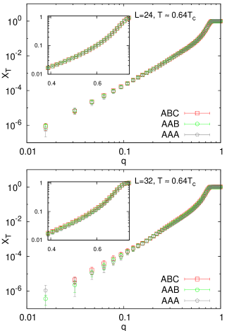
Figure 1: (Color online) The quantity $X_{\text{T}}$ as defined in the text, as a function of $q$ for lattice size $L=24$ (top) and $L=32$ (bottom) at temperature $T\simeq 0.64T_{\text{c}}$. Insets show a magnified view of the region $q\sim 0.6$ (log-log plot). Plots show data for $X_{\text{T}}$ computed only with triplets of independent configurations (ABC), with triplets in which two configurations belong to the same Monte Carlo history (AAB), and triplets in which all configurations come from the same Monte Carlo history (AAA). No significant difference shows up as long as we take enough uncorrelated configurations from the same replica.

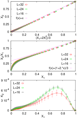
Figure 2: (Color online) Top: $X_{2}$ as a function of the corresponding polynomial in $X_{1}$ (Eq. (18)). The straight line is the theoretical prediction (unit slope). Center: the ratio $X_{2}/X_{1}$ as a function of $X_{1}$, where the straight line is the theoretical prediction. Bottom: the squared difference $K_{2}=\left[X_{2}-(X_{1}+2X_{1}^{2})/3\right]^{2}$ as function of $X_{1}$. Data refer to $T\sim 0.64T_{\text{c}}$

For models in which the overlap is not fluctuating in the large-volume limit (i.e., $P(q)$ is a delta function) the above relations are satisfied but reduce to trivial identities. If the replica symmetry is broken, then stochastic stability imposes strong constraints on the form of the overlap matrix and consequently on the overlap probability densities. Ultrametricity is a further simplification: lack of this property might indicate that more than one overlap might be needed to describe the equilibrium configurations PRJPA .

We can extract further information from the distribution $\Pi_{q}(x)$. It has been found MPSTV ; MPV ; MPR that in mean-field theory the probability distribution $\pi(y)$ of the random variable $Y_{J}=1-X_{J}$ behaves as a power law for $Y_{J}\sim 1$. This implies that $\Pi_{q}(x)$ also follows a power law for small $x$ values

$$\pi_{q}(y\rightarrow 1) \sim (1-y)^{x(q)-1}\ \ ,$$

$$\Pi_{q}(s\rightarrow 0) \sim s^{x(q)-1}\ \ .$$ (21)

Since for most samples the $P_{J}(q)$ is a superposition of narrow peaks around sample-dependent $q$ values, separated by wide $q$ intervals in which $P_{J}$ is exactly zero, when dealing with data from simulations of finite-size systems, it is convenient to turn to the cumulative distribution of the $X_{J}$ to improve the statistical signal, especially at small $q$ values:

$$\Pi_{q}^{C}(s)=\int_{0}^{s}dx\Pi_{q}(x)$$ (22)

which should verify at small $s$

$$\Pi_{q}^{C}(s\rightarrow 0)\sim s^{x(q)}\ ;$$ (23)

the probability of finding a sample in which the overlap probability distribution $P_{J}(q)$ in the interval $\left[0,q\right]$ is small enough to verify $\int_{-q}^{q}P(q^{\prime})dq^{\prime}<s$ goes to zero as a power law of $s$.

III.1 Numerical results

We recall that in our simulations we tailored the temperature range for the parallel tempering implementation to improve its performance as discussed in Ref. EAPTJANUS, . This brought us to direct measurements of observables at temperature sets that were not perfectly overlapping at all lattice sizes. In what follows we compare data at temperatures that are slightly different for different lattice sizes. Considering that even if the simulations were performed at exactly the same temperatures, tiny size-dependent critical effects may always affect the results, we preferred not to perform involved interpolations to correct for order $1\%$ or less of temperature discrepancies. In what follows we will refer to the set of data at $T\sim 0.64T_{\text{c}}$ and $T\sim 0.75T_{\text{c}}$ for the sake of brevity; the precise values of the temperatures are summarized in Table 2. We also compare data at exactly $T=0.625=0.57T_{\text{c}}$ for lattice sizes $L=8,16,24$.

As our simulations were not optimized to study the critical region, we take the value $T_{\text{c}}=1.109(10)$ from Refs. HPV1, and HPV2, (featuring many more samples and small sizes to control scaling corrections). Still, combining the critical exponents determination of these references with the Janus data used herein, we obtain a compatible value of $1.105(8)$. DTC2

$L$	$T\sim 0.57T_{\text{c}}$	$T\sim 0.64T_{\text{c}}$	$T\sim 0.75T_{\text{c}}$
8	0.625	$-$	0.815
16	0.625	0.698	0.844
24	0.625	0.697	0.842
32	$-$	0.703	0.831

Table 2: Temperature values for each lattice size ($T_{\text{c}}=1.109$ HPV1 ; HPV2 ).

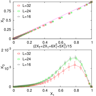
Figure 3: (Color online) Data at $T\sim 0.64T_{\text{c}}$. Top: $X_{3}$ as a function of the corresponding polynomial in $X_{1}$ and $X_{\text{T}}$ (Eq. (19)). The straight line is the theoretical prediction (unit slope). Bottom: the squared difference $K_{3}=\left[X_{3}-(2X_{\text{T}}+2X_{1}+6X_{1}^{2}+5X_{1}^{3})/15\right]^{2}$ as function of $X_{1}$, $T=0.64T_{\text{c}}$. Lines connecting points are only a guide to the eye.

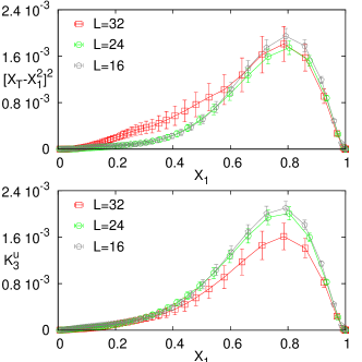
Figure 4: (Color online) Top: The squared difference $\left[X_{\text{T}}-X_{1}^{2}\right]^{2}$ as a function of $X_{1}$. Bottom: the quantity $K_{3}^{u}=\left[X_{3}-(2X_{1}+8X_{1}^{2}+5X_{1}^{3})/15\right]^{2}$ as a function of $X_{1}$. All data for $T\sim 0.64T_{\text{c}}$ and for lattice sizes $L=16,24,32$. The lines connecting the data points are only intended as a guide to the eye.

We simulated four independent real replicas per sample: thus we avoid any bias in computing $X_{\text{T}}(q)$, Eq. (17), by picking three configurations in three distinct replicas. We show the computed $X_{\text{T}}(q)$ for the largest lattices $L=24$ and $L=32$ in Fig. 1 i) considering only configurations for different replicas (data labeled as ABC); ii) picking two configurations out of three from the same replica (labeled AAB); iii) picking the three configurations in the same replica (labeled AAA) . To minimize the effect of bias due to hard samples, we picked up the same number of configurations per sample, spaced in time by an amount proportional to the exponential autocorrelation time $\tau_{\text{exp}}$ of that sample EAPTJANUS . The three data sets (ABC, AAB, AAA) are equivalent and small deviations at low $q$ values remain within error bars: this is a strong indication of the statistical quality of our data, as described in Ref. EAPTJANUS, .

We now come to test the Ghirlanda-Guerra relations, Eqs. (18) and (19). Plotting the two sides of Eq. (18) parametrically in $q$, the data show a slight deviation from the theoretical prediction (see Fig. 2 top). It is interesting to compare the discrepancies for different lattice sizes. As the position and width of $P(q)$ are size-dependent, it seems more natural to compare functions of the moments $X_{k}$ for different lattice sizes as functions of the integrated probability $x(q)=X_{1}(q)$ (see Fig. 2 middle). It is evident from the third plot in Fig. 2 that the quantity

$$K_{2}=\left[X_{2}-(X_{1}+2X_{1}^{2})/3\right]^{2}$$ (24)

is definitely non-zero although very small in the entire range. However, the data are compatible with $K_{2}$ decreasing with lattice size and becoming null in the $L\to\infty$ limit.

We can reach similar conclusions regarding $X_{3}$ as a function of $X_{\text{T}}$ and $X_{1}$, and the quantity

$$K_{3}=\left[X_{3}-(2X_{\text{T}}+2X_{1}+6X_{1}^{2}+5X_{1}^{3})/15\right]^{2}$$ (25)

(see Fig. 3). Even if the data for different lattice sizes stand within a couple of standard deviations, there is a clear improvement in the agreement between the prediction and the Monte Carlo data as the size increases.

The data plotted in Fig. 4 take into account the ultrametric relation (20). When comparing $X_{\text{T}}$ and $X_{1}^{2}$ small deviations from the prediction arise. However, data for $L=32$ have strong fluctuations, and do not hint at any clear tendency with the system size. The bottom plot in Fig. 4 shows data for the quantity

$$K_{3}^{u}=\left[X_{3}-(2X_{1}+8X_{1}^{2}+5X_{1}^{3})/15\right]^{2},$$ (26)

which we obtain by substituting (20) in  (25). The same considerations we made above apply here: the agreement with ultrametric relations (19) and (20) improves with increasing $L$.

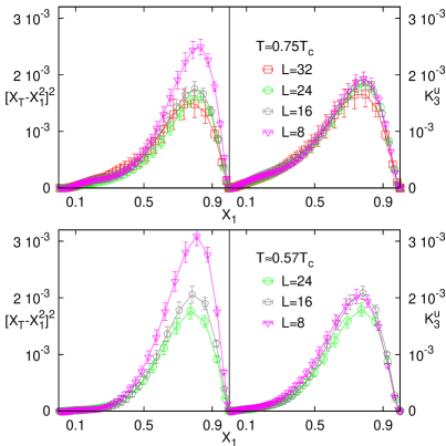
Figure 5: (Color online) Square difference $\left[X_{\text{T}}-X_{1}^{2}\right]^{2}$ (left) and the quantity $K_{3}^{u}=\left[X_{3}-(2X_{1}+8X_{1}^{2}+5X_{1}^{3})/15\right]^{2}$ (right) as a function of $X_{1}$. Top: for $T=0.75T_{\text{c}}$ and $L=8,16,24,32$. Bottom: for $T=0.57T_{\text{c}}$ and $L=8,16,24$.

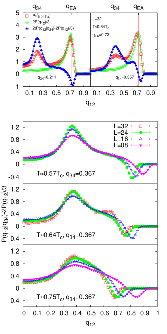
Figure 6: (Color online) Top: The conditioned probability $P(q_{12}|q_{34})$ (open squares) for $L=32$ and $T\sim 0.64T_{\text{c}}$ and two values of $q_{34}=0.211$ (left) and $q_{34}=0.367$ (right). We also plot $2P(q_{12})/3$ (open circles) and the difference (full triangles) of the two above quantities (Eq. (27) in the text), scaled by a factor $2$ for a better view. $q_{34}$ and $q_{\text{EA}}$ values are indicated by vertical lines for visual reference. We took the value $q_{\text{EA}}(L=32,T=0.64T_{\text{c}})\sim 0.72$ as given in Ref. EAPTJANUS, .
Bottom: The difference $P(q_{12}|q_{34})-2P(q_{12})/3$ with $q_{34}=0.367$, for different lattice size compared at temperatures $T=0.75T_{\text{c}}$, $T=0.64T_{\text{c}}$, $T=0.57T_{\text{c}}$.

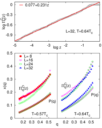
Figure 7: (Color online) Asymptotic behavior of the cumulative probability $\Pi_{q}^{C}(z)$ (Eq. (23)). Top: small-$z$ decay for $L=32$, $T=0.64T_{\text{c}}$ and $q=0.3125$. Bottom: comparison of the exponent $x(q)$ obtained by the two methods described in the text (uppermost data points represent values obtained by fitting $\Pi_{q}^{C}(z)$, lowermost data points come from integrating the $P(q)$), for some lattice sizes, many cut-off values $q$ and temperatures $T\sim 0.57T_{\text{c}}$ (left) and $T\sim 0.64T_{\text{c}}$ (right).

We can compare the results above with those of Ref. MPR, , in which a good agreement between theoretical prediction of the kind of Eqs. (18), (19), (20) and Monte Carlo data on $3D$ Edwards-Anderson spin glass with Gaussian couplings was reported, but without clear evidence on whether the very small discrepancies could be controlled or not in the limit of large volume. In this respect, we have been able to thermalize systems of linear sizes up to twice the largest lattice studied in Ref. MPR, and these larger sizes show a trend towards satisfying Eqs. (18), (19), (20) that was not clear in Ref. MPR, . We also note that finite-size effects are stronger at low temperatures, and obtaining evidence of the correct trend requires data from simulations of larger systems than at higher temperature. We can also compare data at $T\sim 0.75T_{\text{c}}$ and $T=0.57T_{\text{c}}$ (we have data at exactly $T=0.625$ for lattice sizes $L=8$, $L=16$ and $L=24$ but unfortunately not for $L=32$). We see that at $T\sim 0.75T_{\text{c}}$ the data for the squared differences $K_{3}^{u}$ and $\left[X_{\text{T}}-X_{1}^{2}\right]^{2}$ are almost size-independent (this is actually true for $\left[X_{\text{T}}-X_{1}^{2}\right]^{2}$ when $L>8$, see Fig. 5, top). At $T\sim 0.64T_{\text{c}}$ (see Fig. 4), such effects cannot be clearly told by comparing only the smallest lattices considered, $L=16$ and $L=24$. At $T=0.57T_{\text{c}}$, size-dependent effects are strong even for $L=16,24$ (see Fig. 5, bottom).

Having data from four independent replicas per sample, we have access to the joint probability of two independent overlaps. According to Eq. (8) the quantity

$$\frac{P(q_{12},q_{34})}{P(q_{34})}-\frac{2}{3}P(q_{12})=P(q_{12}|q_{34})-\frac{2}{3}P(q_{12})\ ,$$ (27)

(where $P(\cdot|\cdot)$ denotes conditional probability) when plotted versus $q_{12}$, should be a delta function in $q_{34}$. This quantity is shown for $L=32$, $T\sim 0.64T_{\text{c}}$ and two values of $q_{34}$ in the top plot of Fig. 6 and reveals a clear peak around $q_{34}$. At high $q_{12}$ values there is a small excess in the probability $P(q_{12})\,P(q_{34})$, so the difference in Eq. (27) becomes negative. As one sees in Fig. 6 this happens at values $q_{12}\gtrsim q_{\text{EA}}$, i.e., in a region of atypically large overlaps that should vanish in the thermodynamical limit. The size dependence for the quantity in Eq. (27) is not easy to quantify from the data: as one can see in Fig. 6 (bottom) for a particular choice of $q_{34}$, the peak height tends to increase with $L$ (at least for $T\sim 0.75T_{\text{c}}$), but in a very slow way, making extrapolations in the $L\to\infty$ limit practically impossible. Despite this, we note that the negative peaks get narrower as the system size increases: we expect then that this effect will disappear at larger system sizes.

We conclude this section commenting the asymptotic behavior of the cumulative probability $\Pi_{q}^{C}(z)$, Eq. (23). The small-$z$ decay is clearly a power law (see top plot in Fig. 7), but the best fit exponent is significantly different from the estimate obtained by integrating the overlap distribution $P(q)$. Fig. 7 shows a comparison of the exponent $x(q)$ obtained by the two methods, for some lattice sizes, many cut-off values $q$ and two temperatures, $T\sim 0.64T_{\text{c}}$ and $T\sim 0.57T_{\text{c}}$. Although the differences seem to decrease by increasing the lattice size, the trend is very slow and even not in a clear direction for some values of the cutoff $q$. Again, the only conclusion that can be drawn is that the finite-size effects are large, even for $L=32$, and safe extrapolations in the $L\to\infty$ limit cannot be done.

A closer inspection of the data reported in Fig. 7 reveals that the difference between the two data sets is roughly a constant, and this difference becomes extremely important in the limit of small $q$, where one would expect both measurements of $x(q)$ to approach zero. Contrary to expectations, the $x(q)$ estimated from the data of $\Pi^{C}_{q}$ seems to remain non-zero even in the $q\to 0$ limit. A possible explanation for this observation comes from the fact that the delta peaks in the $P_{J}(q)$ get broader for systems of finite size. Indeed, in the thermodynamic limit, one would expect $P_{J}(q)$ to be the sum of delta functions centered on overlap values extracted from the average distribution $P_{\infty}(q)$: if this expectation is true, then the value for $X_{J}(q)$ is nothing but the probability of having a peak at an overlap value smaller than $q$ and this is exactly $x(q)$. However, if the delta peaks acquire a non-zero width $\Delta$ due to finite-size effects, then for $q<\Delta$ the overlap probability distribution close to the origin $P_{J}(0)$ may be affected by broad peaks centered on overlaps larger than $q$, which should not count in the thermodynamical limit. If this explanation is correct, then the limit $q\to 0$ for the data shown in Fig. 7 (bottom) obtained from $\Pi^{C}_{q}$ should give a rough estimate, in the large $L$ limit, for the peak width $\Delta$ (see data in Table 2 and discussion below).

IV THE ORDER PARAMETER DISTRIBUTION

$L$	$T/T_{\text{c}}$	$q_{\text{EA}}$	$x_{\infty}(q_{\text{EA}})$	$\Delta$
32	0.75	0.663(19)	0.91(13)	0.0923(80)
	0.64	0.7319(30)	0.828(28)	0.1015(30)
24	0.75	0.69674(72)	1.0000(3)	0.10618(84)
	0.64	0.7625(27)	0.876(24)	0.1182(24)
	0.57	0.7954(24)	0.842(25)	0.1216(32)
16	0.75	0.73780(73)	1.000031(7)	0.1443(10)
	0.64	0.809(16)	1.00(14)	0.150(11)
	0.57	0.8210(41)	0.811(49)	0.1683(51)
8	0.75	0.8250(21)	1.000001(9)	0.2872(37)
	0.57	0.886(18)	0.95(18)	0.296(28)
$L$	$T/T_{\text{c}}$	$\alpha$	$\gamma$	$\chi^{2}/\text{d.o.f.}$
32	0.75	1.92(34)	11.2(1.2)	20/97
	0.64	0.93(44)	7.7(1.0)	38/103
24	0.75	2.04(21)	9.68(55)	45/101
	0.64	0.95(21)	6.88(41)	69/107
	0.57	0.75(17)	5.62(30)	88/110
16	0.75	1.76(16)	5.14(31)	77/107
	0.64	0.45(21)	4.50(52)	133/113
	0.57	0.53(19)	3.37(40)	161/115
8	0.75	0.73(22)	2.02(34)	501/121
	0.57	0.49(16)	1.36(17)	466/123

Table 3: Results of the fitting procedure of Eq. (36) on numerical $P(q)$ data, with kernel exponent $k=2.5$ (see Eq. (33)). All errors on parameters are jackknife estimates. 

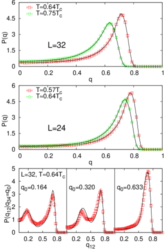
Figure 8: (Color online) Comparison between the Monte Carlo data of the $P(q)$ and the convolution computed as described in the text (solid lines). Top: $L=32$, $T\sim 0.64T_{\text{c}}$ and $T\sim 0.75T_{\text{c}}$. Center: $L=24$, $T\sim 0.57T_{\text{c}}$ and $T\sim 0.64T_{\text{c}}$. Bottom: the conditioned probability $P(q_{12}|q_{34}=q_{0})$ for $L=32$, $T\sim 0.64T_{\text{c}}$ and some values of $q_{0}$.

We now compare the $P(q)$ obtained in numerical simulations of the three-dimensional Edwards-Anderson model (1) to the prediction obtained by smoothly introducing controlled finite-size effects on a mean-field-like distribution consisting in a delta function centered in $q=q_{\text{EA}}$ and a continuous tail down to $q=0$ (a similar analysis has been carried out for long-range spin-glass models, see Ref. LR, ). On the positive $q$ axis one has

$$P_{\infty}(q) = \widetilde{P}(q)\Theta(q_{\text{EA}}-q)$$ (28)

$$+ [1-x_{\infty}(q_{\text{EA}})]\delta(q-q_{\text{EA}})\;,$$

$$x_{\infty}(q_{\text{EA}}) = \int_{0}^{q_{\text{EA}}}dq\,\widetilde{P}(q)\;.$$ (29)

It is convenient to introduce the effective field $h$ trough

$$q=\tanh\left(h\right)$$ (30)

and consider its distribution

$$\mathcal{P}_{\infty}(h) = P_{\infty}\big{(}q(h)\big{)}\frac{dq(h)}{dh}$$ (31)

$$= \frac{dq(h)}{dh}\widetilde{P}\big{(}q(h)\big{)}\Theta(h_{\text{EA}}-h)+$$

$$[1-x_{\infty}(q_{\text{EA}})]\delta(h-h_{\text{EA}})\;,$$

$$x_{\infty}(q_{\text{EA}}) = \int_{0}^{h_{\text{EA}}}dh\widetilde{\mathcal{P}}(h)\;,$$ (32)

being clear that $q_{\text{EA}}=\tanh\left(h_{\text{EA}}\right)$. This change of variable smooths the constraint on the fluctuations of $q$ near the extremes of the distribution.

In a finite-size system the thermodynamical distribution $\mathcal{P}_{\infty}(h)$ will be modified, mainly by the fact that delta functions become distributions with non-zero widths. Remember that, in the thermodynamical limit, we expect the distribution $\mathcal{P}_{J}(h)$ for any given sample to be the sum of delta functions. A simple way to take into account the spreading of the delta functions due to finite-size effects is to introduce a symmetric convolution kernel

$$G^{(k)}_{\Delta}(h-h^{\prime})\equiv C\exp{\left[-\left(\left|h-h^{\prime}\right|/\Delta\right)^{k}\right]}\;,$$ (33)

where $C$ is a normalizing constant and the spreading parameter $\Delta$ is assumed not to depend on $h$,  while it should have a clear dependence on the system size, such that $\lim_{L\to\infty}\Delta=0$. The parameter $k$, to be varied in the interval $[2,3]$, is introduced in order to consider convolutions different from the Gaussian case ($k=2$).

In order to obtain an analytic expression for the finite size distribution

$$\mathcal{P}_{L}(h)\equiv\int dh^{\prime}\frac{\mathcal{P}_{\infty}(h^{\prime})+\mathcal{P}_{\infty}(-h^{\prime})}{2}G^{(k)}_{\Delta}(h-h^{\prime})\;,$$ (34)

we assume the following form for the continuous part of the distribution

$$\widetilde{\mathcal{P}}(h)\equiv\widetilde{P}\big{(}q(h)\big{)}\frac{dq(h)}{dh}=\widetilde{P}(0)(1+\alpha h^{2}+\gamma h^{4})\;,$$ (35)

where $\widetilde{\mathcal{P}}(0)=\widetilde{P}(0)=P_{\infty}(0)$, $\alpha$ and $\gamma$ are free parameters to be inferred from the data. The final result is

$$\mathcal{P}_{L}(h) = [1-x_{\infty}(q_{\text{EA}})]\frac{G^{(k)}_{\Delta}(h-h_{\text{EA}})+G^{(k)}_{\Delta}(h+h_{\text{EA}})}{2}$$ (36)

$$+ \widetilde{P}(0)\int_{-h_{\text{EA}}}^{h_{\text{EA}}}\!\!\!\!\!\!dz\,\left[1+\alpha z^{2}+\gamma z^{4}\right]G^{(k)}_{\Delta}(h-z)$$

where $x_{\infty}(q_{\text{EA}})=2\widetilde{P}(0)[h_{\text{EA}}+\alpha h_{\text{EA}}^{2}/3+\gamma h_{\text{EA}}^{5}/5]$.

We let $\alpha$, $\gamma$, $q_{\text{EA}}$ and $\Delta$ vary in a fitting procedure to $P(q)$ Monte Carlo data; values of $\widetilde{P}(0)$ are fixed to the Monte Carlo values $P_{MC}(0)$. The choice of the exponent $k$ in the convolution kernel is crucial. We varied $k$ in the interval $\left[2,3\right]$. The Gaussian convolution $k=2$ turned out to be the worst choice in such interval, giving rise to unphysical negative weights for the delta function contributions, i.e., $1-x_{\infty}(q_{\text{EA}})<0$. We obtained very good results with the choice $k=2.5$. Fit parameters are reported in Table 2 for some lattice sizes and temperatures, while Fig. 8 shows comparison between Monte Carlo $P(q)$ and the relative fitting curve. Although the fitting curves interpolate nicely the numerical $P(q)$, some of the fitting parameters may look strange: in particular $q_{\text{EA}}$ is a bit larger than the peak location and $x_{\infty}(q_{\text{EA}})\simeq 1$ (for example, in the $L=32$ data the difference is around $2\%$). It is worth remembering that in the solution of the SK model at low temperatures the continuous part $\mathcal{P}(q)$ has a divergence for $q\to q_{\text{EA}}^{-}$, which can easily dominate the delta function in finite-size systems (where delta peaks are broadened). Indeed, by increasing the system size, $q_{\text{EA}}$ seems to move towards the location of the peak maximum and $x_{\infty}(q_{\text{EA}})$ becomes smaller than 1.

In order to make a stronger test of the above fitting procedure, we have used the fit parameters in Table 2 to derive the finite-size conditional probability

$$P_{L}(q|q^{\prime})=P_{L}(q,q^{\prime})/P_{L}(q^{\prime})$$ (37)

applying the convolution kernel $G^{(k)}_{\Delta}(h-h^{\prime})$ to the $L=\infty$ joint probability given by the Ghirlanda-Guerra relation, r.h.s of Eq.(8). Fig. 8 shows a comparison between our extrapolated $P_{L}(q_{12}|q_{34}=q_{0})$ and the Monte Carlo data for $L=32$, $T=0.64T_{\text{c}}$ and three values of $q_{0}$: the agreement is very good at any value of $q_{0}$, especially considering that the fitting parameters were previously fixed by interpolating the unconditional overlap distribution $P_{L}(q)$.

V CONCLUSIONS

We performed a direct inspection of stochastic stability and ultrametricity properties on the sample-to-sample fluctuations of the overlap probability densities obtained by large-scale Monte Carlo simulations of the three-dimensional Edwards-Anderson model. We found small but still sizeable deviations from the prediction of the Ghirlanda-Guerra relations but a clear tendency towards improvement of agreement with increasing system size.

Large fluctuations make it difficult to draw any definitive conclusion on the analysis of the ultrametric relation (20) when taking into account data for the largest lattice size. In addition, critical effects show up at $T\sim 0.75T_{\text{c}}$. Considering that for a stochastically stable system overlap equivalence is enough to infer ultrametricity, the results presented here support and integrate the analyses and claims of Refs janusPRL, ,  EAPTJANUS, and  ContucciPRL, , in which the authors reported strong evidence of overlap equivalence.

We also turned our attention to the shape of the overlap probability distribution, showing that finite-size $P_{L}(q)$ and $P_{L}(q,q^{\prime})$ compare well with mean-field (infinite-size) predictions, modified by finite-size effects that only make delta functions broad.

- (1) D. Sherrington and S. Kirkpatrick, Phys. Rev. Lett. 35 1792 , (1975).
- (2) G. Parisi, J.Phys.A: Math. Gen., 13, 1101 (1980).
- (3) M. Mézard, G. Parisi and M.A. Virasoro, Spin Glass Theory and Beyond 1987 World Scientific, Singapore.
- (4) D.S. Fisher and D.A. Huse, Phys. Rev. Lett. 56 1601 (1986); Phys. Rev. B 38 373 (1988); Phys. Rev. B 38 386 (1988).
- (5) E. Marinari, G. Parisi, F. Ricci-Tersenghi, J.J. Ruiz-Lorenzo and F. Zuliani J. Stat. Phys. 98, 973 (2000).
- (6) Auditya Sharma and A.P. Young, Phys. Rev. B 84, 014428 (2011)
- (7) F. Guerra, Int. J. Mod. Phys. B 10, 1675 (1997).
- (8) M. Aizenman and P. Contucci, J. Stat. Phys. 92, 765 (1998).
- (9) S. Ghirlanda and F. Guerra, J. Phys. A: Math. Gen. 31 9149 (1998).
- (10) G. Parisi, available as preprint cond-mat/9801081.
- (11) M. Talagrand, Ann. Math. 163, 221 (2006).
- (12) The Janus Collaboration: F. Belletti, M. Cotallo, A. Cruz, L. A. Fernandez, A. Gordillo, A. Maiorano, F. Mantovani, E. Marinari, V. Martin-Mayor, A. Muñoz-Sudupe, D. Navarro, S. Perez-Gaviro, J. J. Ruiz-Lorenzo, S. F. Schifano, D. Sciretti, A. Tarancon, R. Tripiccione and J. L. Velasco, Comp. Phys. Comm. 178, 208 (2008).
- (13) F. Belletti, M. Cotallo, A. Cruz, L.A. Fernandez, A. Gordillo-Guerrero, M. Guidetti, A. Maiorano, F. Mantovani, E. Marinari, V. Martin-Mayor, A. Munoz Sudupe, D. Navarro, G. Parisi, S. Perez-Gaviro, J.J. Ruiz-Lorenzo, S.F. Schifano, D. Sciretti, A. Tarancon, R. Tripiccione, J.L. Velasco, and D. Yllanes, Phys. Rev. Lett. 101, 157201 (2008); F. Belletti, A. Cruz, L.A. Fernandez, A. Gordillo-Guerrero, M. Guidetti, A. Maiorano, F. Mantovani, E. Marinari, V. Martin-Mayor, J. Monforte, A. Muñoz-Sudupe, D. Navarro, G. Parisi, S. Perez-Gaviro, J.J. Ruiz-Lorenzo, S.F. Schifano, D. Sciretti, A. Tarancon, R. Tripiccione and D. Yllanes, J. Stat. Phys., 135, 1121 (2009).
- (14) Janus Collaboration: R. Alvarez Banos, A. Cruz, L.A. Fernandez, J. M. Gil-Narvion, A. Gordillo-Guerrero, M. Guidetti, A. Maiorano, F. Mantovani, E. Marinari, V. Martin-Mayor, J. Monforte-Garcia, A. Munoz Sudupe, D. Navarro, G. Parisi, S. Perez-Gaviro, J. J. Ruiz-Lorenzo, S.F. Schifano, B. Seoane, A. Tarancon, R. Tripiccione, D. Yllanes, J. Stat. Mech. P06026 (2010).
- (15) F. Krzakala and O.C. Martin, Phys. Rev. Lett. 85, 3013 (2000).
- (16) Edwards F. S. and Anderson P. W., J. Phys. F 5 975, (1974); J. Phys. F. 6, 1927, (1976).
- (17) K. Hukushima and K. Nemoto, J. Phys. Soc. Japan, 65, 1604 (1996).
- (18) E. Marinari, Optimized Monte Carlo Methods, in Advances in Computer Simulation, Ed. J. Kerstesz and I. Kondor, (Springer-Verlag, 1998).
- (19) L.A. Fernandez, V. Martin-Mayor, S. Perez-Gaviro, A. Tarancon, A.P. Young, Phys. Rev. B 80 024422 (2009).
- (20) D. Amit and V. Martin-Mayor, Field Theory, the Renormalization Group and Critical Phenomena, World Scientific, Singapore (2005).
- (21) A. Sokal, Functional Integration: Basics and Applications, edited by C. DeWitt-Morette, P. Cartier, and A. Folacci, Plenum, New York (1997).
- (22) D. Iñiguez, G. Parisi and J.J. Ruiz-Lorenzo, J. Phys. A.: Math. Gen, 29, 4337 (1996).
- (23) G. Parisi and F. Ricci-Tersenghi, J. Phys. A: Math. Gen. 33, 113 (2000).
- (24) G.G. Athanasiu, C.P. Bachas and W.F. Wolff, Phys. Rev. B 35, 1965 (1987).
- (25) P Contucci, C. Giardinà, C. Giberti, G. Parisi, and C. Vernia, Phys. Rev. Lett. 99, 057206 (2007).
- (26) M. Mézard, G. Parisi, N. Sourlas, G. Toulouse, and M. Virasoro, Phys. Rev. Lett. 52, 1156 (1984)
- (27) M. Mézard, G. Parisi and M.A. Virasoro, J. Physique Lett. 46, 217 (1985).
- (28) E. Marinari, G. Parisi and J.J. Ruiz-Lorenzo, Phys. Rev. B. 58, 14852 (1998).
- (29) M. Hasenbusch, A. Pelissetto and E. Vicari, J. Stat. Mech L02001 (2008).
- (30) M. Hasenbusch, A. Pelissetto and E. Vicari, Phys. Rev. B 78, 214205 (2008).
- (31) A. Billoire, L. A. Fernandez, A. Maiorano, E. Marinari, V. Martin-Mayor, D. Yllanes, J. Stat. Mech. P10019 (2011).
- (32) L. Leuzzi, G. Parisi, F. Ricci-Tersenghi and J.J. Ruiz-Lorenzo, Phys. Rev. Lett. 101, 107203 (2008).