Relay Selection with Channel Probing in Sleep-Wake Cycling Wireless Sensor Networks

Abstract

In geographical forwarding of packets in a large wireless sensor network (WSN) with sleep-wake cycling nodes, we are interested in the local decision problem faced by a node that has “custody” of a packet and has to choose one among a set of next-hop relay nodes to forward the packet towards the sink. Each relay is associated with a “reward” that summarizes the benefit of forwarding the packet through that relay. We seek a solution to this local problem, the idea being that such a solution, if adopted by every node, could provide a reasonable heuristic for the end-to-end forwarding problem. Towards this end, we propose a relay selection problem comprising a forwarding node and a collection of relay nodes, with the relays waking up sequentially at random times. At each relay wake-up instant the forwarder can choose to probe a relay to learn its reward value, based on which the forwarder can then decide whether to stop (and forward its packet to the chosen relay) or to continue to wait for further relays to wake-up. The forwarder’s objective is to select a relay so as to minimize a combination of waiting-delay, reward and probing cost. Our problem can be considered as a variant of the asset selling problem studied in the operations research literature. We formulate our relay selection problem as a Markov decision process (MDP) and obtain some interesting structural results on the optimal policy (namely, the threshold and the stage-independence properties). We also conduct simulation experiments and gain valuable insights into the performance of our local forwarding-solution.

I Introduction

Consider a wireless sensor network deployed for the detection of rare events, e.g., forest fires, intrusion in border areas, etc. To conserve energy, the nodes in the network sleep-wake cycle whereby they alternate between an ON state and a low power OFF state. We are further interested in asynchronous sleep-wake cycling where the point processes of wake-up instants of the nodes are not synchronized [1, 2].

In such networks, whenever an event is detected, an alarm packet (containing the event location and a time stamp) is generated and has to be forwarded, through multiple hops (as illustrated in Fig. 1), to a control center (sink) where appropriate action could be taken. Since the network is sleep-wake cycling, a forwarding node (i.e., a node holding an alarm packet) has to wait for its neighbors to wake-up before it can choose one for the next hop. Thus, due to the sleep-wake process, there is a delay incurred at each hop en-route to the sink, and our interest is in minimizing the total average end-to-end delay subject to a constraint on some global metric of interest such as the average hop count, or the average total transmission power (sum of the transmission power used at each hop). Such a global problem can be considered as a stochastic shortest path problem [3], for which the distributed Bellman-Ford algorithm (e.g., the LOCAL-OPT algorithm proposed by Kim et al. in [1]) can be used to obtain the optimal solution. However, a major drawback with such an approach is that a pre-configuration phase is required to run such algorithms, which would involve exchange of several control messages. Furthermore, such global configuration would need to be performed each time there is a change in the network topology, such as due to node failures, or variations in the propagation characteristics, etc.

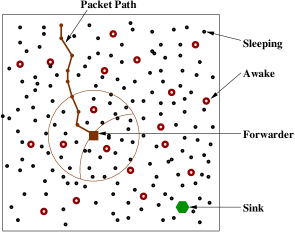
Figure 1: Illustration of a packet being forwarded to the sink node (green hexagon) through a sleep-wake cycling network. The square node (labeled as forwarder) is the current custodian of the packet.

The focus of our research is instead towards designing simple forwarding rules that use only the local information available at a forwarding node. In our own earlier work in this direction [4, 2], we formulated the local forwarding problem as one of minimizing the one-hop forwarding delay subject to a constraint on the reward offered by the chosen relay. The reward associated with a relay is a function of the transmission power and the progress towards the sink made by the packet when forwarded via that relay. We considered two variations of the problem, one in which the number of potential relays is known [4], and the other in which only a probability mass function of the number of potential relays is known [2]. In each case, we derived the structure of the optimal policy. Further, through simulation experiments we found that, in some region of operation, the end-to-end performance (i.e., total delay and total transmission power) obtained by applying the solution to the local problem at each hop is comparable with that obtained by the global solution (i.e., the LOCAL-OPT proposed by Kim et al. [1]), thus providing additional support for the approach of utilizing local forwarding rules, albeit suboptimal.

In our earlier work, however, we assume that the gain of the wireless communication channel between the forwarding node and a relay is a deterministic function of the distance between the two, whereas, in practice, due to the phenomenon called shadowing, the channel gain at a given distance from the forwarding node is not a constant, but varies spatially over points at the same distance (the variation being typically modeled as log normally distributed [5]). In addition to not being just a function of distance, the path-loss between a pair of locations varies with time; in a forest, for example, this would be due to seasonal variations in the foliage. Therefore, in each instance that a node gets custody of a packet, the node has to send probe packets to determine the channel gain to relay nodes that wake up, and thereby “offer” to forward the packet. Such probing incurs additional cost (for instance, see [6] where probing allows the transmitter to obtain a finer estimate of the channel gain). Hence, “to probe” or “not to probe” can itself become a part of the decision process. In the current work we incorporate these features (namely, channel probing and the associated power cost) while choosing a relay for the next hop, leading to an interesting variant of the asset selling problem [7, Section 4.4], [8] studied in the operations research literature.

Outline and Our Contributions: In Section II we will formally describe our system model, following which we will discuss the related work. Sections III and IV are devoted towards characterizing the structure of the policy RST-OPT (ReSTricted-OPTimal) which is optimal within a restricted class of relay selection policies. In Section V we will discuss the globally optimal GLB-OPT policy. Numerical and simulation results are presented in Section VI. Our main technical contributions are the following:

• We characterize the optimal policy, RST-OPT, in terms of stopping sets. We prove that the stopping sets have a threshold structure (Theorem 1).

• We further prove that the stopping sets are identical across the decision stages (Theorem 2 and 3). This result can be considered as a generalization of the one-step-look ahead rule (see the remark following Theorem 2).

• Through one-hop numerical work we find that the performance of RST-OPT is close to that of GLB-OPT. This result is useful because, the sub-optimal RST-OPT is computationally more simpler than GLB-OPT. We have also conducted simulations to study the end-to-end performance of RST-OPT.

We will finally conclude in Section VII. For the ease of readability we have moved most of the proofs to the Appendix.

II System Model: The Relay Selection Problem

We will describe the system model from the context of geographical forwarding, also known as location aware routing, [4, 9, 10]. In geographical forwarding it is assumed that each node in the network knows its location (with respect to some reference) as well as the location of the sink.

Figure 2: The hatched area is the forwarding region $\mathcal{L}$. For $\ell\in\mathcal{L}$, the progress $Z_{\ell}$ is the difference between the forwarder-to-sink and $\ell$-to-sink distances.

Consider a forwarding node $\mathscr{F}$ located at $v$ (see Fig. 2). The sink node is situated at $v_{0}$. Thus, the distance between $\mathscr{F}$ and the sink is $V=\ \parallel v-v_{0}\parallel$ (we use $\parallel\cdot\parallel$ to denote the Euclidean norm). The communication region is the set of all locations where reliable exchange of control messages (transmitted using a low rate robust modulation technique on a separate control channel) can take place between $\mathscr{F}$ and a receiver, if any, at these locations. In Fig. 2 we have shown the communication region to be circular, but in practice this region can be arbitrary. The set of nodes within the communication region are referred to as the neighbors.

Let $V_{\ell}=\ \parallel\ell-v_{0}\parallel$ represent the distance of a location $\ell$ (which is a point in $\Re^{2}$) from the sink. Now define the progress of location $\ell$ as $Z_{\ell}=V-V_{\ell}$, which is simply the difference between the $\mathscr{F}$-to-sink and $\ell$-to-sink distances. $\mathscr{F}$ is interested in forwarding the packet only to a neighbor within the forwarding region $\mathcal{L}$, which is defined as

$$\mathcal{L}=\Big{\{}\ell\in\mbox{communication region}:Z_{\ell}\geq z_{min}\Big{\}}$$ (1)

where, $z_{min}>0$ is the minimum progress constraint (see Fig. 2, where the hatched area is the forwarding region). The reason for using $z_{min}>0$ in the definition of $\mathcal{L}$ are: (1) practically this will ensure that a progress of at least $z_{min}$ is made by the packet at each hop, and (2) mathematically this condition will allow us to bound the reward functions (to be defined sooner) to take values within an interval $[0,\overline{r}]$.

Next, it is natural to assume that $\mathcal{L}$ is bounded; we will further assume that $\mathcal{L}$ is closed. The reason for imposing this condition will become clear in Section IV. Finally, we will refer to the nodes in the forwarding region as relays.

Sleep-Wake Process: Without loss of generality, we will assume that $\mathscr{F}$ receives an alarm packet (from an upstream node) at time $0$, which has to be forwarded to one of the relays. There are $N$ relays that wake-up sequentially at the points of a Poisson process of rate $\frac{1}{\tau}$. The wake-up times are denoted, $0\leq W_{1}\leq\cdots\leq W_{N}$. The relay waking up at the instant $W_{k}$ is referred to as the $k$-th relay. Let $U_{1}=W_{1}$ and $U_{k}=W_{k}-W_{k-1}$ $(k=2,\cdots,N$) denote the inter-wake-up time between the $k$-th and the $(k-1)$-th relay. Then, $\{U_{k}\}$ are i.i.d. exponential random variables with mean $\tau$.

Channel Model: We will consider the following standard model for the transmission power required by $\mathscr{F}$ to achieve an SNR (signal to noise ratio) constraint of $\Gamma$ at some location $\ell$, whose distance from $\mathscr{F}$ is more than $d_{ref}$ (far-field reference distance beyond which the following expression will hold [12]):

$$P_{\ell}=\frac{\Gamma N_{0}}{G_{\ell}}{\left(\frac{D_{\ell}}{d_{ref}}\right)}^{\xi}$$ (2)

where, $D_{\ell}=\ \parallel\ell-v\parallel$ is the distance between $\mathscr{F}$ and $\ell$, $G_{\ell}$ is the random component of the channel gain between $\mathscr{F}$ and $\ell$, $N_{0}$ is the receiver noise variance, and $\xi$ is the path-loss attenuation factor. We will assume that $d_{ref}\leq z_{min}$ so that $P_{\ell}$ in (2) is the power required for any $\ell\in\mathcal{L}$. Also, for simplicity, from here on we will use $\Gamma^{\prime}$ to denote $\frac{\Gamma N_{0}}{d_{ref}^{\xi}}$.

Although $G_{\ell}$ along with the path-loss, ${\left(\frac{D_{\ell}}{d_{ref}}\right)}^{\xi}$, constitutes the gain of the channel, for simplicity we will throughout refer to $G_{\ell}$ itself as the channel gain between $\mathscr{F}$ and the location $\ell$. We will assume that the set of channel gains, $\{G_{\ell}:\ell\in\mathcal{L}\}$, are i.i.d. We will further assume that the channel coherence time is large so that the channels gains remain unchanged over the entire duration of the decision process, i.e., in physical layer wireless terminology, we have a slowly varying channel.

Remark: There are two remarks we would like to make here. First is regarding the channel gains being i.i.d. Since the randomness in the channel is spatially correlated [13], if two locations $\ell$ and $u$ are very close then the corresponding gains, $G_{\ell}$ and $G_{u}$, will not be independent; a minimum separation between the receivers is required for the gains to be statistically independently. Thus, our assumption of independence between the channel gains to the relays requires that the relays should not be close to each other, or, equivalently, the relay density should not be large. We will assume that this physical property holds, and, thus, proceed with the technical assumption that the channel gains are i.i.d.

Next, about the slowly varying channel, it suffices for the channel coherence time to be longer than the sleep-wake cycling period (recall footnote 1 from page 1). Under our light traffic assumption where the events are rare, with a probability close to $1$, a node wakes up and finds no forwarding node in its communication range. Thus, with a high probability, when a node wakes up, it stays awake for a few milliseconds, e.g., $3$ milliseconds (for sending a control packet, turning the radio from send to listen, and then waiting for a possible response). Thus, for example, with a $1\%$ duty cycle, the inter-wakeup time would need to be $300$ milliseconds, imposing a reasonable requirement on the channel coherence time.

Reward Structure: Finally, combining progress, $Z_{\ell}$, and power, $P_{\ell}$, we define the reward associated with a location $\ell\in\mathcal{L}$ as,

$$R_{\ell}=\frac{Z_{\ell}^{a}}{P_{\ell}^{(1-a)}}=\frac{Z_{\ell}^{a}}{(\Gamma^{\prime}D_{\ell}^{\xi})^{(1-a)}}G_{\ell}^{(1-a)},$$ (3)

where $a\in[0,1]$ is used to trade-off between $Z_{\ell}$ and $P_{\ell}$. The reward being inversely proportional to $P_{\ell}$ is clear because it is advantageous to use low power to get the packet across; $R_{\ell}$ is proportional to $Z_{\ell}$ to promote progress towards the sink while choosing a relay for the next hop.

The channel gains, $\{G_{\ell}\}$, are non-negative; we will further assume that they are bounded above by $g_{max}$. These conditions along with $Z_{\ell}\geq z_{min}$ (which implies that $D_{\ell}\geq z_{min}$) and $\mathcal{L}$ is bounded (so that $Z_{\ell}\leq z_{max}$ for all $\ell\in\mathcal{L}$) will provide the following upper bound for the reward functions $\Big{\{}R_{\ell}:\ell\in\mathcal{L}\Big{\}}$:

$$\overline{r} = \frac{z_{max}^{a}}{(\Gamma^{\prime}z_{min}^{\xi})^{(1-a)}}g_{max}^{(1-a)}.$$

Thus, the reward values lie within the interval $[0,\overline{r}]$.

Let $F_{\ell}$ represent the c.d.f. (cumulative distribution function) of $R_{\ell}$, and

$$\mathcal{F} = \Big{\{}F_{\ell}:\ell\in\mathcal{L}\Big{\}}$$ (4)

denote the collection of all possible reward distributions. From (3), note that, given a location $\ell$ it is only possible to know the reward distribution $F_{\ell}$. To know the exact reward $R_{\ell}$, $\mathscr{F}$ has to transmit probe packets to learn the channel gain $G_{\ell}$ (we will formalize probing very soon).

Relay Locations: We will assume that each of the $N$ relays is randomly and mutually independently located in the forwarding region $\mathcal{L}$. Formally, if $L_{1},L_{2},\cdots,L_{N}$ denotes the relay locations, then these are i.i.d. uniform over the forwarding set $\mathcal{L}$ (this assumption holds if the nodes are deployed according to a spatial Poisson process). Let $L$ denote the uniform distribution over $\mathcal{L}$ so that, for $k=1,2,\cdots,N$, the distribution of $L_{k}$ is $L$.

Remark: Although, for the sake of motivating the model, we have restricted to a very specific $\mathcal{F}$ (set of reward distributions) and $L$ (relay location distribution), it is important to note that all our analysis in the subsequent sections will follow through for more general $\mathcal{F}$ and $L$ as well.

At time $0$, $\mathscr{F}$ only knows that there are $N$ relays in its forwarding set $\mathcal{L}$, but does not know their locations, $L_{k}$, nor their channel gains, $G_{L_{k}}$.

Sequential Decision Problem: When the $k$-th relay wakes up, we assume that its location $L_{k}$, and hence its reward distribution $F_{L_{k}}$ is revealed to $\mathscr{F}$. This can be accomplished by including the location information $L_{k}$ within a control packet (sent using a low rate robust modulation technique, and hence, assumed to be error free) transmitted by the $k$-th relay upon waking up. However, if $\mathscr{F}$ wishes to learn the channel gain $G_{L_{k}}$ (and hence the exact reward value $R_{L_{k}}$), it has to transmit additional probe packets (indeed several packets) in order to obtain a reliable estimate of the channel gain, incurring a power cost of $\delta\geq 0$ units. Thus, when the $k$-th relay wakes up (referred to as stage $k$), given the set of previously probed and unprobed relays (i.e., the history), the actions available to $\mathscr{F}$ are:

• s: stop and forward the packet to a relay with the maximum reward (best relay) among the probed relays; with this action the decision process ends.

• c: continue to wait for the next relay to wake-up (average waiting time is $\tau$); with this action the decision process enters stage $k+1$.

• p: probe a relay from the set of all unprobed relays (provided there is at least one unprobed relay). The probed relay’s reward value is then revealed, allowing $\mathscr{F}$ to update the best relay. After probing, the decision process is still at stage $k$ and $\mathscr{F}$ has to again decide upon an action.

In the model, for the sake of analysis, we neglect the time taken for the exchange of control packets and the time taken to probe a relay to learn its channel gain. We argue that this is reasonable for very low duty cycling networks, where the average inter-wake-up time is much larger than the time taken for probing and for the exchange of control packets.

At stage $k$, let $b_{k}$ denote the reward of the best relay, and $\mathcal{F}_{k}$ be the vector of reward distribution of the unprobed relays, i.e., formally,

$$b_{k}=\max\Big{\{}R_{L_{i}}:i\leq k,\mbox{ relay }i\mbox{ has been probed}\Big{\}},$$

and

$$\mathcal{F}_{k}=\Big{(}F_{L_{i}}:i\leq k,\mbox{ relay }i\mbox{ is unprobed}\Big{)}.$$

We will regard $(b_{k},\mathcal{F}_{k})$ to be the state of the system at stage $k$. Note that, it is possible that until stage $k$ no relay has been probed, in which case $b_{k}=-\infty$, or all the relays are probed so that $\mathcal{F}_{k}$ is empty. Whenever $\mathcal{F}_{k}$ is empty we will represent the state as simply $b_{k}$. Now we can define a forwarding policy $\pi$ as follows:

Definition 1

A policy $\pi$ is a sequence of mappings $(\mu_{1},\mu_{2},\cdots,\mu_{N})$ where,

• for $k=1,2,\cdots,N-1$, $\mu_{k}(b_{k},\mathcal{F}_{k})\in\{\textsf{s},\textsf{c},\textsf{p}\}$ and $\mu_{k}(b_{k})\in\{\textsf{s},\textsf{c}\}$, and

• $\mu_{N}(b_{N},\mathcal{F}_{N})\in\{\textsf{s},\textsf{p}\}$ and $\mu_{N}(b_{N})\in\textsf{s}$.

Note that the action to continue is not available at the last stage $N$. Let $\Pi$ denote the set of all policies. $\blacksquare$

For a policy $\pi\in\Pi$, the delay incurred, denoted $D$, is the time until a relay is chosen. Let $R$ denote the reward offered by the chosen relay. Further, let $M$ denote the total number of relays that were probed during the decision process. Then, recalling that $\delta$ is the probing cost, $\delta M$ represents the total cost of probing. We would like to think of $(R-\delta M)$ as the effective reward achieved using policy $\pi$. Then, denoting $\mathbb{E}[\cdot]$ to be the expectation operator conditioned on using policy $\pi$, the problem we are interested in is the following:

$$\mbox{Minimize}_{\pi\in\Pi}\ \bigg{(}\mathbb{E}_{\pi}[D]-\eta\Big{(}\mathbb{E}_{\pi}[R]-\delta\mathbb{E}_{\pi}[M]\Big{)}\bigg{)},$$ (5)

where $\eta>0$ is the multiplier used to trade-off between delay and effective reward.

Restricted Class $\overline{\Pi}$: Recall that the state at stage $k$ is of the form $(b_{k},\mathcal{F}_{k})$ where $\mathcal{F}_{k}$ is the set of all unprobed relays. The size of $\mathcal{F}_{k}$ can vary from $0$ (if all the $k$ relays that have woken up thus far have been probed) to $k$ (if none have been probed). Further, suppose the size of $\mathcal{F}_{k}$ is $m$ ($0<m\leq k$) then $\mathcal{F}_{k}\in\mathcal{F}^{m}$ (the $m$ times Cartesian product of $\mathcal{F}$) since the reward distribution of each unprobed relay can be any distribution from $\mathcal{F}$. Thus, the set of all possible states at stage $k$ is large. Hence, for analytical tractability, we first consider (in Sections III and IV) solving the problem in (5) over a restricted class of policies, $\overline{\Pi}\subseteq\Pi$, where a policy is restricted to take decisions keeping only up to two relays awake $-$ one the best among all probed relays and other the best among the unprobed ones. Thus, the decision at stage $k$ is based on $(b_{k},H_{k})$ where $H_{k}$ is the “best distribution in $\mathcal{F}_{k}$” (our notion of best distribution is based on stochastic ordering; we will formally discuss this in Section IV). Later in Section V we will discuss the optimal policy within the unrestricted class of policies $\Pi$.

Related Work: Suppose the probing cost $\delta=0$, then the objective in (5) will reduce to minimizing $\Big{(}\mathbb{E}_{\pi}[D]-\eta\mathbb{E}_{\pi}[R]\Big{)}$. Further, when $\delta=0$, since there is no advantage in not probing, an optimal policy is to always probe relays as they wake-up so that their reward value is immediately revealed to $\mathscr{F}$. Alternatively, if $\mathscr{F}$ is not allowed to exercise the option to not-probe a relay, then again the model reduces to the case where the relay rewards are immediately revealed as and when they wake-up.

We have studied this particular case of our relay selection problem (which we will refer to as the basic relay selection model) in our earlier work [2, Section 6],[4], and this basic model can be shown to be equivalent to a basic version of the asset selling problem [7, Section 4.4], [8] studied in the operations research literature. The asset selling problem comprises a seller (with some asset to sell) and a collection of buyers who are arriving sequentially in time. The offers made by the buyers are i.i.d. If the seller wishes to choose an early offer, then he can invest the funds received for a longer time period. On the other hand, waiting could yield a better offer, but with the loss of time during which the sale-proceeds could have been invested. The seller’s objective is to choose an offer so as to maximize his final revenue (received at the end of the investment period). Thinking of the offer of a buyer as analogous to the reward of a relay, the seller’s objective of maximizing revenue is equivalent to the forwarder’s objective of minimizing a combination of delay and reward.

However, in the present work we generalize this basic version by allowing the probing cost to be positive (i.e., $\delta>0$) so that a relay’s reward value (equivalently, buyer’s offer value) is not revealed to the forwarder (equivalently, seller) for free. Instead the forwarder can choose to probe a relay to know its reward value after incurring an additional cost of $\delta$. Although there is work reported in the asset selling problem literature which is centered around the idea of the offer (or reward) distribution being unknown, or not knowing a parameter of the offer distribution [14, 15] but these do not incorporate an additional probe action like in our model here. To the best of our knowledge, the particular class of models we study here is not available in the asset selling problem literature.

Problem of choosing a next-hop relay arises in the context of geographical forwarding (as mentioned earlier, geographical forwarding [9, 16] is a forwarding technique where the prerequisite is that the nodes know their respective locations as well as the sink’s location). For instance, Zorzi and Rao in [10] propose an algorithm called GeRaF (Geographical Random Forwarding) which, at each forwarding stage, chooses the relay making the largest progress. For a sleep-wake cycling network, Liu et al. in [17] propose a relay selection approach as a part of CMAC, a protocol for geographical packet forwarding. Under CMAC, node $i$ chooses an $r_{0}$ that minimizes the expected normalized latency (which is the average ratio of one-hop delay and progress). Links to more literature on similar work from the context of geographical forwarding can be found in [2]. However, these work do not incorporate the action of “probing a relay” as in our relay selection model here.

From the context of wireless communication, the action to probe generally occurs in the problem of channel selection [18, 19]. For instance, the authors in [18] study the following problem: a transmitter, aiming to maximize its throughput, has to choose a channel for its transmissions, among several available ones. The transmitter, only knowing the channel gain distributions, has to send probe packets to learn the exact channel state information (CSI). Probing many channels yields a channel with a good gain but reduces the effective time for transmission within the channel coherence period. The problem is to obtain optimal strategies to decide when to stop probing and to transmit. An important difference with our work is that, in [18, 19] all the channel gain distributions are known a priori while here the reward distributions are revealed as and when the relays wake-up. We will discuss more about the work in [18] in Section V.

Another work which is close to ours is that of Stadje [20], where only some initial information about an offer (e.g., the average size of the offer) is revealed to the decision maker upon its arrival. In addition to the actions, stop and continue, the decision maker can also choose to obtain more information about the offer by incurring a cost. Recalling previous offers is not allowed. A similar problem is studied by Thejaswi et al. in [6], where initially a coarse estimate of the channel gain is made available to the transmitter. The transmitter can choose to probe the channel a second time to get a finer estimate. In both of these [20, 6], the optimal policy is characterized by a threshold rule. However, the horizon length of these problems is infinite, because of which the thresholds are stage independent. In general, for a finite horizon problem the optimal policy would be stage dependent. For our problem, despite being a finite horizon one, we are able to show that certain stopping sets are identical across stages. This is due to the fact that we allow the best probed relay to stay awake.

III Restricted Class $\overline{\Pi}$: An MDP Formulation

Confining to the restricted class $\overline{\Pi}$, in this section we will formulate the problem in (5) as a Markov decision process. This will require us to first discuss the one-step cost functions and state transitions before proceeding to write the Bellman optimality equations.

III-A One-Step Costs and State Transitions

The decision instants or the decision stages are the times at which the relays wake-up. Thus, there are $N$ decision stages indexed by $k=1,2,\cdots,N$. Recall that for any policy in the restricted class $\overline{\Pi}$, the decision at stage $k$ is based on $(b_{k},H_{k})$, where $b_{k}$ is the best reward so far and $H_{k}\in\mathcal{F}_{k}$ is the best reward distribution with $\mathcal{F}_{k}$ being the set of reward distributions of all the unprobed relays so far. As mentioned earlier, if no relay has been probed until stage $k$ then $b_{k}=-\infty$. On the other hand, if all the relays have been probed, in which case $\mathcal{F}_{k}$ is empty, then we will denote the state as simple $b_{k}$. Hence, the state space can be written as,

$$\mathcal{X} = [0,\overline{r}]\cup\Big{\{}(b,F_{\ell}):b\in\{-\infty\}\cup[0,\overline{r}],\ell\in\mathcal{L}\Big{\}}\cup\{\textbf{\emph{t}}\}$$

where t is the cost-free termination state. We will use $(b,F_{\ell})$ to denote a generic state at stage $k$.

Now, at stage $k=1,2,\cdots,N-1$, given that the state is $(b,F_{\ell})$, if $\mathscr{F}$’s decision is to stop then the decision process enters t, with $\mathscr{F}$ incurring a termination cost of $-\eta b$ (recall from (5) that $\eta>0$ is the trade-off parameter). On the other hand, if the action is to continue then $\mathscr{F}$ will first incur a waiting cost of $U_{k+1}$ (the time until the next relay wakes up) and then, when the $(k+1)$-th relay wakes-up (whose reward distribution is $F_{L_{k+1}}$), $\mathscr{F}$ chooses between the two unprobed relays $-$ one the previous relay with reward distribution $F_{\ell}$, and other the new one with distribution $F_{L_{k+1}}$ $-$ so that the state at stage $k+1$ will be either $(b,F_{\ell})$ or $(b,F_{L_{k+1}})$. The best reward value continues to be $b$ since no new relay has been probed during the state transition.

Alternatively, $\mathscr{F}$ could choose the action to probe the available unprobed relay (whose reward distribution is $F_{\ell}$) incurring a cost of $\eta\delta$ (recall that $\delta$ is the probing cost). After probing, the decision process is still considered to be at stage $k$ with the new state being $b^{\prime}=\max\{b,R_{\ell}\}$, where $R_{\ell}$ is the reward value of the just probed relay (thus the distribution of $R_{\ell}$ is $F_{\ell}$). $\mathscr{F}$ has to now further decide whether to stop (incurring a one-step cost of $-\eta b^{\prime}$ and enter t), or continue (in which case the one-step cost is $U_{k+1}$ and the next state is $(b^{\prime},F_{L_{k+1}})$).

Summarizing the above we can write the one-step cost, when the state at stage $k$ is $(b,F_{\ell})$, as

$$g_{k}\Big{(}(b,F_{\ell}),a_{k}\Big{)} = \left\{\begin{array}[]{cl}-\eta b&\mbox{ if }a_{k}=\textsf{s}\\ U_{k+1}&\mbox{ if }a_{k}=\textsf{c}\\ \eta\delta&\mbox{ if }a_{k}=\textsf{p}.\end{array}\right.$$

The next state, $X^{\prime}$, is given by

$$X^{\prime} = \left\{\begin{array}[]{cl}\textbf{\emph{t}}&\mbox{ if }a_{k}=\textsf{s}\\ (b,F_{\ell})\mbox{ or }(b,F_{L_{k+1}})&\mbox{ if }a_{k}=\textsf{c}\\ \max\{b,R_{\ell}\}&\mbox{ if }a_{k}=\textsf{p}.\end{array}\right.$$

We have used $X^{\prime}$ to denote the next state instead of $X_{k+1}$ because, if $a_{k}=\textsf{p}$ then the system is still at stage $k$. Only when the action is s or c the system transits to the stage $k+1$.

Next, if the state at stage $k$ is $b$ (states of this form occur after probing the available unprobed relay; recall the above expressions when $a_{k}=\textsf{p}$), then

$$g_{k}(b,a_{k}) = \left\{\begin{array}[]{cl}-\eta b&\mbox{ if }a_{k}=\textsf{s}\\ U_{k+1}&\mbox{ if }a_{k}=\textsf{c},\end{array}\right.$$

and the next state is

$$X_{k+1} = \left\{\begin{array}[]{cl}\textbf{\emph{t}}&\mbox{ if }a_{k}=\textsf{s}\\ (b,F_{L_{k+1}})&\mbox{ if }a_{k}=\textsf{c}.\end{array}\right.$$

The action to probe is not available whenever the state is $b$.

At the last stage $N$, action c is not available, so that

$$g_{N}(b,F_{\ell}) = \left\{\begin{array}[]{cl}-\eta b&\mbox{ if }a_{k}=\textsf{s}\\ \eta\delta&\mbox{ if }a_{k}=\textsf{p},\end{array}\right.$$

with the system entering t if $a_{k}=\textsf{s}$, otherwise (i.e., if $a_{k}=\textsf{p}$) the state transits to $\max\{b,R_{k}\}$. Finally, $g_{N}(b)=-\eta b$. Note that for a policy $\pi$, the expected sum of all the one-step costs starting from stage $1$, plus the average waiting time for the first relay, $\mathbb{E}[U_{1}]=\tau$, will equal the total cost in (5).

III-B Cost-to-go Functions and the Bellman Equation

Let $J_{k}$, $k=1,2,\cdots,N$, represent the optimal cost-to-go function at stage $k$. Thus, $J_{k}(b)$ and $J_{k}(b,F_{\ell})$ denote the cost-to-go, depending on whether there is, or is not an unprobed relay. For the last stage, $N$, we have, $J_{N}(b)=-\eta b$, using which we obtain,

$$J_{N}(b,F_{\ell}) = \min\Big{\{}-\eta b,\eta\delta+\mathbb{E}_{\ell}\Big{[}J_{N}(\max\{b,R_{\ell}\})\Big{]}\Big{\}}$$ (11)

$$= \min\Big{\{}-\eta b,\eta\delta-\eta\mathbb{E}_{\ell}\Big{[}\max\{b,R_{\ell}\}\Big{]}\Big{\}},$$

where $\mathbb{E}_{\ell}[\cdot]$ denotes the expectation with respect to (w.r.t.) $R_{\ell}$ whose distribution is $F_{\ell}$. The first term in the $\min$-expression above is the cost of stopping and the second term is the expected cost of probing and then stopping (recall that action c is not available at the last stage $N$). Next, for stages $k=1,2,\cdots,N-1$, denoting the expectation w.r.t. the distribution, $L$, of the location, $L_{k+1}$, of the next relay by $\mathbb{E}_{L}[\cdot]$, we have

$$J_{k}(b) = \min\Big{\{}-\eta b,\tau+\mathbb{E}_{L}\Big{[}J_{k+1}(b,F_{L_{k+1}})\Big{]}\Big{\}},$$ (12)

and

$$J_{k}(b,F_{\ell}) = \min\Big{\{}-\eta b,\eta\delta+\mathbb{E}_{\ell}\Big{[}J_{k}(\max\{b,R_{\ell}\})\Big{]},$$ (13)

$$\tau+\mathbb{E}_{L}\Big{[}\min\{J_{k+1}(b,F_{\ell}),J_{k+1}(b,F_{L_{k+1}})\}\Big{]}\Big{\}}.$$

The first term in both the min-expressions above is the cost of stopping. The middle term in (13) is the expected cost of probing, with $\eta\delta$ being the one-step cost and the remaining term being the future cost. The last term in both expressions is the expected cost of continuing, with $\tau$ representing the mean waiting time until the next relay wakes up. The future cost-to-go in the last term of (13) can be understood as follows. When the state at stage $k=1,2,\cdots,N-1$ is $(b,F_{\ell})$ and, if $\mathscr{F}$ decides to continue, then the reward distribution of the next relay is $F_{L_{k+1}}$. Now, given the distributions $F_{\ell}$ and $F_{L_{k+1}}$, if $\mathscr{F}$ is asked to retain one of them, then it is optimal to go with the distribution that fetches a lower cost-to-go from stage $k+1$ onwards, i.e., it is optimal to retain $F_{\ell}$ if $J_{k+1}(b,F_{\ell})\leq J_{k+1}(b,F_{L_{k+1}})$, otherwise retain $F_{L_{k+1}}$. Later in this section we will show that, given two distributions, $F_{\ell}$ and $F_{u}$, if $F_{\ell}$ is stochastically greater than $F_{u}$ [21] then $J_{k+1}(b,F_{\ell})\leq J_{k+1}(b,F_{u})$ (see Lemma 2-(i)) so that it is optimal to retain the stochastically greater distribution.

First, for simplicity let us introduce the following notation. For $k=1,2,\cdots,N-1$, let $C_{k}$ represent the cost of continuing:

$$C_{k}(b) = \tau+\mathbb{E}_{L}\Big{[}J_{k+1}(b,F_{L_{k+1}})\Big{]}$$ (14)

$$C_{k}(b,F_{\ell})=\tau+\mathbb{E}_{L}\Big{[}\min\{J_{k+1}(b,F_{\ell}),J_{k+1}(b,F_{L_{k+1}})\}\Big{]}.$$ (15)

For $k=1,2,\cdots,N$, the cost of probing, $P_{k}$, is given by

$$P_{k}(b,F_{\ell}) = \eta\delta+\mathbb{E}_{\ell}\Big{[}J_{k}(\max\{b,R_{\ell}\})\Big{]}.$$ (16)

From (14) and (15) it is immediately clear that $C_{k}(b,F_{\ell})\leq C_{k}(b)$ for any $F_{\ell}$ ($\ell\in\mathcal{L}$). This inequality should be intuitive as well, since $\mathscr{F}$ can expect to accrue a better cost if, in addition to a probed relay, it also possesses an unprobed relay. It will be useful to note this inequality as a lemma.

Lemma 1

For $k=1,2,\cdots,N-1$ and any $(b,F_{\ell})$ we have $C_{k}(b,F_{\ell})\leq C_{k}(b)$.

Proof:

As discussed just before the Lemma statement, the inequality follows easily from the expressions of these costs; recall (14) and (15). ∎

Finally, using the above cost notation, the cost-to-go functions in (12) and (13) can be written as, for $k=1,2,\cdots,N-1$,

$$J_{k}(b) = \min\Big{\{}-\eta b,C_{k}(b)\Big{\}}$$ (17)

$$J_{k}(b,F_{\ell}) = \min\Big{\{}-\eta b,P_{k}(b,F_{\ell}),C_{k}(b,F_{\ell})\Big{\}}.$$ (18)

III-C Ordering Results for the Cost-to-go Functions

We will examine how the cost-to-go functions $J_{k}(b)$ and $J_{k}(b,F_{\ell})$ behave as functions of $F_{\ell}$ and the stage index $k$. We will first require the definition of stochastic ordering.

Definition 2 (Stochastic Ordering)

Given two distributions $F_{\ell}$ and $F_{u}$, $F_{\ell}$ is stochastically greater than $F_{u}$, denoted as $F_{\ell}\geq_{st}F_{u}$, if $1-F_{\ell}(r)\geq 1-F_{u}(r)$, for all $r$. Equivalently [21], $F_{\ell}\geq_{st}F_{u}$ if and only if for every non-decreasing function $f:\Re\rightarrow\Re$, $\mathbb{E}_{\ell}[f(R_{\ell})]\geq\mathbb{E}_{u}[f(R_{u})]$ where the distributions of $R_{\ell}$ and $R_{u}$ are $F_{\ell}$ and $F_{u}$, respectively. $\blacksquare$

Now, consider two relays at locations $\ell$ and $u$. If the corresponding reward distributions, $F_{\ell}$ and $F_{u}$, are such that $F_{\ell}\geq_{st}F_{u}$ then $\mathscr{F}$ can expect that probing the relay at $\ell$ would yield a better reward value than the relay at $u$. Thus, $\mathscr{F}$ would prefer the stochastically greater reward distribution $F_{\ell}$, over $F_{u}$. Extending this observation, it is reasonable to expect that $\mathscr{F}$ can accrue lower expected costs (total, continuing and probing costs) if the unprobed reward distribution available at stage $k$ is $F_{\ell}$ than if it is $F_{u}$. We will formally prove this result next. Also, we will show that the expected cost at stage $k$ is less than that at stage $k+1$, i.e., $J_{k}(x)\leq J_{k+1}(x)$ for any state $x$. This again should be intuitive because, starting from stage $k$, $\mathscr{F}$ has the option to observe an additional relay than if it were to start from stage $k+1$. With more resource available, and with these being i.i.d., $\mathscr{F}$ should achieve a better cost. We will state these two results in the following lemma.

Lemma 2

1. For $k=1,2,\cdots,N-1$, if $F_{\ell}\geq_{st}F_{u}$ then $C_{k}(b,F_{\ell})\leq C_{k}(b,F_{u})$, (and including $k=N$) $P_{k}(b,F_{\ell})\leq P_{k}(b,F_{u})$ and $J_{k}(b,F_{\ell})\leq J_{k}(b,F_{u})$.

2. For $k=1,2,\cdots,N-2$, $C_{k}(b)\leq C_{k+1}(b)$ and $C_{k}(b,F_{\ell})\leq C_{k+1}(b,F_{\ell})$, (and including $k=N-1$) $P_{k}(b,F_{\ell})\leq P_{k+1}(b,F_{\ell})$ and $J_{k}(b,F_{\ell})\leq J_{k+1}(b,F_{\ell})$.

Proof:

To prove (i) we first show that the various costs are non-increasing functions of $b$. We then complete the proof using the definition of stochastic ordering (Definition 2). Part (ii) follows from induction. Detail proofs are available in Appendix A. ∎

IV Restricted Class $\overline{\Pi}$: Structural Results

We begin by defining, at stage $k=1,2,\cdots,N-1$, the stopping set $\mathcal{S}_{k}$ as

$$\mathcal{S}_{k} = \Big{\{}b:-\eta b\leq C_{k}(b)\Big{\}}.$$ (19)

From (17) it follows that the stopping set $\mathcal{S}_{k}$ is the set of all states $b$ (states of this form are obtained after probing at stage $k$) where it is better to stop than to continue.

Similarly, for a given distribution $F_{\ell}$ we define the stopping set $\mathcal{S}_{k}^{\ell}$ as, for $k=1,2,\cdots,N-1$,

$$\mathcal{S}_{k}^{\ell} = \Big{\{}b:-\eta b\leq\min\{P_{k}(b,F_{\ell}),C_{k}(b,F_{\ell})\}\Big{\}}.$$ (20)

Using (18) the set $\mathcal{S}_{k}^{\ell}$ has to be interpreted as, for a given distribution $F_{\ell}$, the set of $b$ such that whenever the state at stage $k$ is $(b,F_{\ell})$ it is better to stop than to either probe or continue. Note that when $b=-\infty$ it is never optimal to stop; hence, both these stopping sets are subsets of $[0,\overline{r}]$. Finally, stopping sets can also be defined for $k=N$ as, $\mathcal{S}_{N}=[0,\overline{r}]$ (since, at the last stage $N$, for any $b$ the only action available is to stop), and

$$\mathcal{S}_{N}^{\ell} = \Big{\{}b:-\eta b\leq P_{k}(b,F_{\ell})\Big{\}}.$$ (21)

The following set inclusion properties easily follow from the definition of these sets and the properties of the cost functions in Lemma 1 and Lemma 2.

Lemma 3

1. For $k=1,2,\cdots,N$ and for any $F_{\ell}$ we have $\mathcal{S}_{k}^{\ell}\subseteq\mathcal{S}_{k}$.

2. For $k=1,2,\cdots,N$, if $F_{\ell}\geq_{st}F_{u}$ then $\mathcal{S}_{k}^{\ell}\subseteq\mathcal{S}_{k}^{u}$.

3. For $k=1,2,\cdots,N-1$ we have $\mathcal{S}_{k}\subseteq\mathcal{S}_{k+1}$, and for any $F_{\ell}$, $\mathcal{S}_{k}^{\ell}\subseteq\mathcal{S}_{k+1}^{\ell}$.

Proof:

Recall the definition of the stopping sets from (19) and (20). Part (i) follows from Lemma 1. Parts (ii) and (iii) are due to Parts (i) and (ii) of Lemma 2, respectively. ∎

Discussion: The above results can be understood as follows. Whenever an unprobed relay (say with reward distribution $F_{\ell}$) is available, $\mathscr{F}$ can be more stringent about the best reward values, $b$, for which it chooses to stop. This is because, $\mathscr{F}$ can now additionally choose to probe $F_{\ell}$ possibly yielding a better reward than $b$. Thus, unless the best reward $b$ is already good (so that there is no gain in probing $F_{\ell}$), $\mathscr{F}$ will not choose to stop. Hence, we have $\mathcal{S}_{k}^{\ell}\subseteq\mathcal{S}_{k}$. Next, if $F_{\ell}\geq_{st}F_{u}$ then since probing $F_{\ell}$ has a higher chance of yielding a better reward, the stopping condition is more stringent if the reward distribution of the available unprobed relay is $F_{\ell}$ than $F_{u}$. Hence, the corresponding stopping sets are ordered as in Part (ii) of the above lemma, i.e., $\mathcal{S}_{k}^{\ell}\subseteq\mathcal{S}_{k}^{u}$. Finally, whenever there are more stages to-go, $\mathscr{F}$ can be more cautious about stopping since it has the option to observe more relays. This suggests that $\mathcal{S}_{k}\subseteq\mathcal{S}_{k+1}$ and $\mathcal{S}_{k}^{\ell}\subseteq\mathcal{S}_{k+1}^{\ell}$.

From our above discussion, the phrase “$\mathscr{F}$ being more stringent about stopping,” suggests that it may be better to stop for larger values of $b$. Equivalently, this would mean that the stopping sets are characterized by thresholds, beyond which it is optimal to stop. This is exactly our first main result (Theorem 1). Later we will prove a more interesting result (Theorem 2 and 3) where we show that the stopping sets are stage independent, i.e., $\mathcal{S}_{k}=\mathcal{S}_{k+1}$ and $\mathcal{S}_{k}^{\ell}=\mathcal{S}_{k+1}^{\ell}$. In the following sub-sections we will work the details of these two results.

IV-A Stopping Sets: Threshold Property

To prove the threshold structure of the stopping sets the following key lemma is required where we show that the increments in the various costs are bounded by the increments in the cost of stopping.

Lemma 4

For $k=1,2,\cdots,N-1$ (for Part (ii), $k=1,2,\cdots,N$), for any $F_{\ell}$, and for $b_{2}>b_{1}$ we have

1. $C_{k}(b_{1})-C_{k}(b_{2})\leq\eta(b_{2}-b_{1})$,

2. $P_{k}(b_{1},F_{\ell})-P_{k}(b_{2},F_{\ell})\leq\eta(b_{2}-b_{1})$

3. $C_{k}(b_{1},F_{\ell})-C_{k}(b_{2},F_{\ell})\leq\eta(b_{2}-b_{1})$.

Proof:

Available in Appendix B. ∎

Theorem 1

For $k=1,2,\cdots,N$ and for $b_{2}>b_{1}$,

1. If $b_{1}\in\mathcal{S}_{k}$ then $b_{2}\in\mathcal{S}_{k}$.

2. For any $F_{\ell}$, if $b_{1}\in\mathcal{S}_{k}^{\ell}$ then $b_{2}\in\mathcal{S}_{k}^{\ell}$.

Proof:

Since $\mathcal{S}_{N}=[0,\overline{r}]$, Part (i) trivially holds for $k=N$. Next, for $k=1,2,\cdots,N-1$, using Lemma 4-(i) we can write,

$$-\eta b_{2}\leq-\eta b_{1}-C_{k}(b_{1})+C_{k}(b_{2}).$$

Since $b_{1}\in\mathcal{S}_{k}$, from (19) we know that $-\eta b_{1}\leq C_{k}(b_{1})$, using which in the above expression we obtain $-\eta b_{2}\leq C_{k}(b_{2})$ implying that $b_{2}\in\mathcal{S}_{k}$. Part (ii) can be similarly completed using Parts (ii) and (iii) of Lemma 4. ∎

Figure 3: Illustration of the threshold property: the vertical lines are the reward axis, with each line corresponding to a different stage. The stopping sets are represented by marking their thresholds on the respective vertical lines.

Discussion: Thus, the stopping sets $\mathcal{S}_{k}$ and $\mathcal{S}_{k}^{\ell}$ can be characterized in terms of lower bounds $\alpha_{k}$ and $\alpha_{k}^{\ell}$, respectively, as illustrated in Fig. 3 (see the vertical line corresponding to the stage index $k$). Also shown in Fig. 3 is the threshold, $\alpha_{k}^{u}$, corresponding to a distribution $F_{u}\leq_{st}F_{\ell}$. From Lemma 3-(i) and 3-(ii) it follows that these thresholds are ordered, $\alpha_{k}\leq\alpha_{k}^{u}\leq\alpha_{k}^{\ell}$. Further, in Fig. 3 we have depicted these thresholds to be decreasing with the stage index $k$ (vertical lines from left to right); this is due to Lemma 3-(iii) from where we know that the stopping sets are increasing with $k$. Our main result in the next section (Theorem 2 and 3) is to show that these thresholds are, in fact, equal (i.e., $\alpha_{k}=\alpha_{k+1}$ and $\alpha_{k}^{\ell}=\alpha_{k+1}^{\ell}$). Finally, note that in Fig. 3 we have not shown the threshold $\alpha_{N}$ corresponding to the stopping set $\mathcal{S}_{N}$; this is simply because $\alpha_{N}=0$ (since $\mathcal{S}_{N}=[0,\overline{r}]$).

IV-B Stopping Sets: Stage Independence Property

From Lemma 3-(iii) we already know that $\mathcal{S}_{k}\subseteq\mathcal{S}_{k+1}$, and $\mathcal{S}_{k}^{\ell}\subseteq\mathcal{S}_{k+1}^{\ell}$. In this section we will prove the inclusion in the other direction, thus leading to the result that the stopping sets are identical across the stages. We will begin by defining the stobing (stopping-or-probing) set $\mathcal{Q}_{k}^{\ell}$ as, for $k=1,2,\cdots,N-1$,

$$\mathcal{Q}_{k}^{\ell} = \Big{\{}b:\min\{-\eta b,P_{k}(b,F_{\ell})\}\leq C_{k}(b,F_{\ell})\Big{\}}.$$ (22)

From (18) it follows that $\mathcal{Q}_{k}^{\ell}$ is, for a given distribution $F_{\ell}$, the set of all $b$ such that whenever the state at stage $k$ is $(b,F_{\ell})$ it is better to either stop or probe than to continue. From the definition of the sets $\mathcal{S}_{k}^{\ell}$ and $\mathcal{Q}_{k}^{\ell}$ (in (20) and (22), respectively) it immediately follows that $\mathcal{S}_{k}^{\ell}\subseteq\mathcal{Q}_{k}^{\ell}$. Also from Lemma 3-(i) we already know that $\mathcal{S}_{k}^{\ell}\subseteq\mathcal{S}_{k}$. However, it is not immediately clear how the sets $\mathcal{Q}_{k}^{\ell}$ and $\mathcal{S}_{k}$ are ordered. We will show that if $\mathcal{F}=\{F_{\ell}:\ell\in\mathcal{L}\}$ is totally stochastically ordered (to be defined next) then $\mathcal{S}_{k}\subseteq\mathcal{Q}_{k}^{\ell}$ (Lemma 7). This result is essential for proving our main theorems.

Definition 3 (Total Stochastic Ordering)

$\mathcal{F}$ is said to be totally stochastically ordered if any two distributions from $\mathcal{F}$ are stochastically ordered. Formally, for any $F_{\ell},F_{u}\in\mathcal{F}$ either $F_{\ell}\geq_{st}F_{u}$ or $F_{u}\geq_{st}F_{\ell}$. Further, if there exists a distribution $F_{m}\in\mathcal{F}$ such that for every $F_{\ell}\in\mathcal{F}$ we have $F_{\ell}\geq_{st}F_{m}$ then we say that $\mathcal{F}$ is totally stochastically ordered with a minimum distribution. $\blacksquare$

Lemma 5

The set of reward distributions $\mathcal{F}$ in (4), is totally stochastically ordered with a minimum distribution.

Proof:

The channel gains, $\{G_{\ell}:\ell\in\mathcal{L}\}$, being identically distributed will be essential to show that $\mathcal{F}$ is totally stochastically ordered. Existence of a minimum distribution will require the assumption we had made earlier (in Section II) that $\mathcal{L}$ is compact (closed and bounded). The complete proof is available in Appendix C. ∎

Remark: Our subsequent results are not simply limited to the $\mathcal{F}$ in (4) which is the distribution set arising from the particular reward structure, $R_{\ell}$, we had assumed in (3). One can consider any collection of bounded reward random variables $\{R_{\ell}\}$, such that the corresponding $\mathcal{F}$ is totally stochastically ordered with a minimum distribution, still all the subsequent results will hold.

Before proceeding to our main theorems, we need the following results.

Lemma 6

Suppose $\mathcal{S}_{k}\subseteq\mathcal{Q}_{k}^{u}$, for some $F_{u}$, and some $k=1,2,\cdots,N-1$. Then for every $b\in\mathcal{S}_{k}$ we have $J_{k}(b,F_{u})=J_{N}(b,F_{u})$.

Proof:

Available in Appendix D. ∎

Next we show that the hypothesis in the above lemma indeed holds for every $F_{\ell}\in\mathcal{F}$.

Lemma 7

For $k=1,2,\cdots,N-1$ and for any $F_{\ell}\in\mathcal{F}$ we have $\mathcal{S}_{k}\subseteq\mathcal{Q}_{k}^{\ell}$.

Proof:

The proof involves two steps:

1) First we show that if there exists an $F_{u}$ such that, for $k=1,2,\cdots,N-1$, $\mathcal{S}_{k}\subseteq\mathcal{Q}_{k}^{u}$ (thus satisfying the hypothesis in Lemma 6), then for every $F_{\ell}\geq_{st}F_{u}$ we have $\mathcal{S}_{k}\subseteq\mathcal{Q}_{k}^{\ell}$. Lemma 6 and the total stochastic ordering of $\mathcal{F}$ are required for this part.

2) Next we show that a minimum distribution $F_{m}$ satisfies the hypothesis in Lemma 6, i.e., for every $k=1,2,\cdots,N-1$, $\mathcal{S}_{k}\subseteq\mathcal{Q}_{k}^{m}$. The proof is completed by recalling that $F_{\ell}\geq_{st}F_{m}$ for every $F_{\ell}\in\mathcal{F}$ and then using in Step 1, $F_{m}$ in the place of $F_{u}$. The existence of a minimum distribution $F_{m}$ (recall Lemma 5) is essential here.

Formal proofs of both steps are available in Appendix E. ∎

The following are the main theorems of this section:

Theorem 2

For $k=1,2,\cdots,N-2$, $\mathcal{S}_{k}=\mathcal{S}_{k+1}$.

Proof:

From Lemma 3-(iii) we already know that $\mathcal{S}_{k}\subseteq\mathcal{S}_{k+1}$. Here, we will show that $\mathcal{S}_{k}\supseteq\mathcal{S}_{k+1}$. Fix a $b\in\mathcal{S}_{k+1}\subseteq\mathcal{S}_{k+2}$. From Lemma 7 we know that $\mathcal{S}_{k+1}\subseteq\mathcal{Q}_{k+1}^{\ell}$ and $\mathcal{S}_{k+2}\subseteq\mathcal{Q}_{k+2}^{\ell}$, for every $F_{\ell}$. Now, applying Lemma 6 we can write, $J_{k+1}(b,F_{\ell})=J_{k+2}(b,F_{\ell})=J_{N}(b,F_{\ell})$. Thus,

$$C_{k+1}(b) = \tau+\mathbb{E}_{L}\Big{[}J_{k+2}(b,F_{L_{k+2}})\Big{]}$$

$$= \tau+\mathbb{E}_{L}\Big{[}J_{k+1}(b,F_{L_{k+1}})\Big{]}$$

$$= C_{k}(b)$$

Finally, since $b\in\mathcal{S}_{k+1}$ we have $-\eta b\leq C_{k+1}(b)=C_{k}(b)$ which implies that $b\in\mathcal{S}_{k}$. ∎

Discussion: It is interesting to compare the above result with the solution obtained for the basic model (i.e., $\delta=0$ case; recall the discussion on related work in Section II) or equivalently the basic asset selling problem [7, Section 4.4]. In [7, Section 4.4], as in our Theorem 2 here, it is shown that similar stopping sets are identical across the stages; this policy is referred to as the one-step-look-ahead rule since the policy, to stop if and only if the “cost of stopping” is less than the “cost of continuing for one-more step and then stopping,” being optimal for stage $N-1$, is optimal for all stages. The key idea there (i.e., in [7, Section 4.4]), as in our Lemma 6, is also to show that the cost-to-go functions, at every stage $k$, are identical for every state within the stopping set. However here, to apply Lemma 6, it was further essential for us to prove Lemma 7 showing that for every $F_{\ell}$, $\mathcal{S}_{k}\subseteq\mathcal{Q}_{k}^{\ell}$. Now, note that the result $\mathcal{S}_{k}\subseteq\mathcal{Q}_{k}^{\ell}$ trivially holds for $\delta=0$, since if $\delta=0$ then for any $(b,F_{\ell})$ it is always optimal to probe, so that $\mathcal{Q}_{k}^{\ell}=[0,\overline{r}]$. Thus, Theorem 2, incorporating the additional case $\delta>0$, can be considered as a generalization of the one-step-look-ahead rule which is optimal for the basic asset selling model.

Theorem 3

For $k=1,2,\cdots,N-1$ and any $F_{\ell}$, $\mathcal{S}_{k}^{\ell}=\mathcal{S}_{k+1}^{\ell}$.

Proof:

Similar to the proof of Theorem 2, here we need to show that the probing and continuing costs satisfy analogous equalities, i.e., for $b\in\mathcal{S}_{k}^{\ell}$ we need to show that $P_{k+1}(b,F_{\ell})=P_{k}(b,F_{\ell})$ and $C_{k+1}(b,F_{\ell})=C_{k}(b,F_{\ell})$. Formal proof is available in Appendix F. ∎

Figure 4: Illustration of the stage independence property: only the thresholds corresponding to the last stage (and stage $N-1$ for $\mathcal{S}_{k}$) are shown, since these alone are sufficient to characterize the stopping sets for any $k$.

Discussion: Owing to Theorem 2 and 3, we can now modify the illustration in Fig. 3 to Fig. 4 where we show only a single threshold corresponding to each stopping set. Thus, to characterize the stopping set $\mathcal{S}_{k}^{\ell}$ for any $k$, it is sufficient to compute only the threshold $\alpha_{N}^{\ell}$ corresponding to the last stage. Similarly, the stopping set $\mathcal{S}_{k}$ is characterized by the threshold $\alpha_{N-1}$ computed for stage $N-1$ (recall that $\alpha_{N}=0$).

IV-C Probing Sets

Similar to the stopping sets $\mathcal{S}_{k}^{\ell}$, one can also define the probing sets $\mathcal{P}_{k}^{\ell}$ as the set of all $b$ such that whenever the state at stage $k$ is $(b,F_{\ell})$ it is better to probe than to either stop or continue, i.e.,

$$\mathcal{P}_{k}^{\ell} = \Big{\{}b:P_{k}(b,F_{\ell})\leq\min\{-\eta b,C_{k}(b,F_{\ell})\}\Big{\}}.$$ (23)

Note that $\mathcal{P}_{k}^{\ell}$ is simply the difference of the sets $\mathcal{Q}_{k}^{\ell}$ and $\mathcal{S}_{k}^{\ell}$, i.e., $\mathcal{P}_{k}^{\ell}=\mathcal{Q}_{k}^{\ell}\setminus\mathcal{S}_{k}^{\ell}$.

From our numerical work we have observed that, similar to the stopping sets, the probing sets $\mathcal{P}_{k}^{\ell}$ are characterized by upper bounds $\zeta_{k}^{\ell}$ (see Fig. 5). The intuition for this is as follows. Let $(b,F_{\ell})$ be the state at stage $N-1$. If the value of $b$ is very small, then it is better to probe than to continue, because probing will give an opportunity to probe an additional relay at stage $N$ in case the process continues after probing at stage $N-1$, while continuing without probing will deprive $\mathscr{F}$ of this opportunity. This argument can be extended to any stage $k$ to conclude that it may be better to probe for small values of $b$. However, as $b$ increases, probing may not yield a better reward than the existing $b$; hence probing might not be worth the cost, so that it may be better to simply continue.

To formally show the threshold property of the probing set $\mathcal{P}_{k}^{\ell}$, the following is sufficient: for any $b_{2}>b_{1}$,

$$P_{k}(b_{1},F_{\ell})-P_{k}(b_{2},F_{\ell}) \leq C_{k}(b_{1},F_{\ell})-C_{k}(b_{2},F_{\ell}).$$

This is because, if $b_{2}\notin\mathcal{S}_{k}^{\ell}$ (so that stopping is not optimal) is such that $b_{2}\in\mathcal{P}_{k}^{\ell}$ (i.e., $P_{k}(b_{2},F_{\ell})\leq C_{k}(b_{2},F_{\ell})$) then from the above inequality we obtain $P_{k}(b_{1},F_{\ell})\leq C_{k}(b_{1},F_{\ell})$, implying that it is optimal to probe at $b_{1}$ as well so that probing sets are characterized by upper bounds. However, we have not yet been able to prove or disprove such a result, but we strongly believe that it is true and make the following conjecture.

Conjecture 1

For $k=1,2,\cdots,N-1$, for any $F_{\ell}$, if $b_{2}\in\mathcal{P}_{k}^{\ell}$ then for any $b_{1}<b_{2}$ we have $b_{1}\in\mathcal{P}_{k}^{\ell}$. $\blacksquare$

Figure 5: Structure of the probing sets if Conjecture 1 is true. 5 Probing sets corresponding to a distribution $F_{\ell}$ such that $\alpha_{N}^{\ell}>\alpha_{N-1}$, 5 Probing sets corresponding to an $F_{u}$ such that $\alpha_{N}^{u}=\alpha_{N-1}$

Discussion: If the above conjecture is true, then some additional structural results can be deduced. For instance, suppose for some $F_{\ell}$, $\alpha_{k}^{\ell}>\alpha_{k}$, or equivalently, $\alpha_{N}^{\ell}>\alpha_{N-1}$ (refer to Fig. 5). Then, since $\mathcal{S}_{k}\subseteq\mathcal{Q}_{k}^{\ell}$ (from Lemma 7), for any $(b,F_{\ell})$ such that $\alpha_{N-1}<b<\alpha_{N}^{\ell}$, it should be optimal to probe. Now, invoking Conjecture 1 we can conclude that it is optimal to probe for any $b<\alpha_{N}^{\ell}$, so that $\zeta_{k}^{\ell}=\alpha_{N}^{\ell}$ for all $k$. Thus, for such “good” distributions, $F_{\ell}$, (i.e., $F_{\ell}$ such that $\alpha_{N}^{\ell}>\alpha_{N-1}$) the policy corresponding to it is completely characterized by a single threshold $\alpha_{N}^{\ell}$. Next, for distributions $F_{u}$ such that $\alpha_{k}^{u}=\alpha_{k}$ (equivalently, $\alpha_{N}^{\ell}=\alpha_{N-1}$; see Fig. 5), there is a window between $\zeta_{k}^{u}$ and $\alpha_{N}^{u}$ where, for any $(b,F_{\ell})$ such that $\zeta_{N}^{u}\leq b<\alpha_{N}^{u}$, it is optimal to continue. Unlike $\alpha_{k}^{u}$, the thresholds $\zeta_{k}^{u}$ are stage dependent. In fact, from our numerical work, we observe that $\zeta_{k}^{u}$ are increasing with $k$. Finally, as depicted in Fig. 5, for any distribution $F_{\ell}$, at the last stage we invariably should have $\alpha_{N}^{\ell}=\zeta_{N}^{\ell}$ since the action to continue is not available at stage $N$.

$$J_{N}(b,\mathcal{H}) = \min\Big{\{}-\eta b,\eta\delta+\min_{F_{\ell}\in\mathcal{H}}\mathbb{E}_{\ell}\Big{[}J_{N}(\max\{b,R_{\ell}\},\mathcal{H}\setminus\{F_{\ell}\})\Big{]}\Big{\}}.$$ (24)

$$J_{k}(b,\mathcal{H}) = \min\Big{\{}-\eta b,\eta\delta+\min_{F_{\ell}\in\mathcal{H}}\mathbb{E}_{\ell}\Big{[}J_{k}(\max\{b,R_{\ell}\},\mathcal{H}\setminus\{F_{\ell}\})\Big{]},\tau+\mathbb{E}_{L}\Big{[}J_{k+1}(b,\mathcal{H}\cup\{F_{L_{k+1}}\})\Big{]}\Big{\}}.$$ (25)

IV-D Policy Implementation

To summarize, from Theorem 1, the stopping sets $\mathcal{S}_{k}$ and $\mathcal{S}_{k}^{\ell}$ are characterized by lower bounds $\alpha_{k}$ and $\alpha_{k}^{\ell}$. In Theorem 2 and 3 we proved that these thresholds are stage independent. Hence it is sufficient to compute only $\alpha_{N-1}$ and $\alpha_{N}^{\ell}$, thus simplifying the overall computation of the optimal policy. Further, if Conjecture 1 is true, then the upper bounds $\zeta_{k}^{\ell}$ are sufficient to characterize the probing sets $\mathcal{P}_{k}^{\ell}$.

Now, $\mathscr{F}$ after computing these thresholds, operates as follows: At stage $k=1,2,\cdots,N-1$, whenever the state is $(b,F_{\ell})$, (1) if $b\geq\alpha_{N}^{\ell}$ then stop and forward the packet to the probed relay, (2) if $b\leq\zeta_{k}^{\ell}$ then probe the unprobed relay and update the best reward to $b^{\prime}=\max\{b,R_{\ell}\}$. Now, if $b^{\prime}\geq\alpha_{N-1}$ stop, otherwise continue to wait for the next relay, (3) otherwise (i.e., if $\zeta_{k}^{\ell}<b<\alpha_{N}^{\ell}$), continue to wait for the next relay to wake-up, at which instant choose, between $F_{\ell}$ and $F_{L_{k+1}}$, whichever is stochastically greater while putting the other unprobed relay to sleep.

If the decision process enters the last stage $N$ and if the state is $(b,F_{\ell})$ then if $b\geq\alpha_{N}^{\ell}$ stop, otherwise probe (continue is not available). Finally, if the state at stage $N$ is $b$ then stop irrespective of its value.

V Unrestricted Class $\Pi$: An Informal Discussion

In this section, based on the insights we have obtained from the analysis in the previous sections, we will informally discuss the possible structure of the optimal policy within the unrestricted class of policies, $\Pi$.

Recall that a policy within $\Pi$, at stage $k$, is in general allowed to base its decision on ($b_{k},\mathcal{F}_{k})$ where $b_{k}$ is the reward of the best probed relay ($b_{k}=-\infty$ if no relay has been probed yet) and $\mathcal{F}_{k}$ is the set of unprobed relays ($\mathcal{F}_{k}=\{\}$ if all the relays have been probed). Thus, the state space at stage $k$ can be written as

$$\mathcal{X}_{k}=\Big{\{}(b,\mathcal{H}):b\in\{-\infty\}\cup[0,\overline{r}],\mathcal{H}\in\mathcal{F}^{j},0\leq j\leq k\Big{\}}.$$ (26)

Again the actions available are stop, probe, and continue. If the action is to probe then $\mathscr{F}$ has to further decide which relay to probe among the several ones available at stage $k$. When there are no unprobed relays (i.e., $\mathcal{H}=\{\ \}$) we will represent the state as simply $b$. We now proceed to write the recursive Bellman optimality equation for this more general unrestricted problem. Although these equations are more involved than the ones in Section III (recall (11) through (13)), these can be understood similarly and hence we do not provide an explanation. The sole purpose for writing these equations here is because we will require these (in Section VI) to perform value iteration and numerically compute an optimal policy for the unrestricted problem. Hence these equations can be omitted without affecting the readability of the remainder of this section.

Let $J_{k}$, $k=1,2,\cdots,N$, represent the optimal cost-to-go at stage $k$ (for simplicity we are again using $J_{k}$), then, $J_{N}(b)=-\eta b$, and $J_{N}(b,\mathcal{H})$ is as in (24). For stage $k=1,2,\cdots,N-1$ we have

$$J_{k}(b) = \min\Big{\{}-\eta b,\tau+\mathbb{E}_{L}\Big{[}J_{k}(b,\{F_{L_{k+1}}\})\Big{]}\Big{\}},$$ (27)

and $J_{k}(b,\mathcal{H})$ as in (25)

In view of the complexity of the problem, we do not pursue the formal analysis of characterizing the structure of the optimal policy within the unrestricted class. However, based on our results from the previous sections and a related work by Chaporkar and Proutiere [18], we will discuss the possible structure of the unrestricted-optimal policy.

V-A Discussion on the Last Stage $N$

Suppose the decision process enters the last stage $N$. Now, given the best reward value among the probed relays, $b$, and the set $\mathcal{H}$ of reward distributions of the unprobed relays, $\mathscr{F}$ has to decide whether to stop, or probe a relay (note that continue action is not available at the last stage). Suppose the action is to probe then, after probing and updating the best reward value, if still there are some unprobed relays left, $\mathscr{F}$ has to again decide to stop or probe. This decision problem is similar to the one studied by Chaporkar and Proutiere in [18], but from the context of channel selection. In the following, we will briefly describe the problem in [18].

Given a set of channels with different channel gain distributions, a transmitter has to choose a channel for its transmissions. The transmitter can probe a channel to know its channel gain. Probing all the channels will enable the transmitter to select the best channel but at the cost of reducing the effective transmission time within the channel coherence period. On the other hand, probing only a few channels may deprive the transmitter of the opportunity to transmit on a better channel. The transmitter is interested in maximizing its throughput within the coherence period.

The authors in [18], for their channel probing problem, prove that the one-step-look-ahead (OSLA) rule is optimal: given the channel gain of the best channel (among the channels probed so far) and a collection of channel gain distributions of the unprobed channels, it is optimal to stop and transmit on the best channel if and only if the throughput obtained by doing so is greater than the expected throughput obtained by probing any unprobed channel and then stopping (by transmitting on the new-best channel). Further, they prove that if the set of channel gain distributions is totally stochastically ordered (recall Definition 3), then it is optimal to probe the channel whose distribution is stochastically largest among all the unprobed channels. However, in their problem maximizing throughput involves optimizing a product of the channel gain and the remaining transmission time, unlike in our problem where (at the last stage) we optimize a linear combination of reward and the probing cost. But, from our numerical work we have seen that a similar OSLA rule is optimal once our decision process enters the last stage $N$: given a state $(b,\mathcal{H})$ at stage $N$, it is optimal to stop if the cost of stopping is less than the cost of probing any distribution from $\mathcal{H}$ and then stopping; otherwise it is optimal to probe the stochastically largest distribution from $\mathcal{H}$.

V-B Discussion on Stages $k=1,2,\cdots,N-1$

For the other stages $k=1,2,\cdots,N-1$, one can begin by defining the stopping sets $\mathcal{S}_{k}$ and $\mathcal{S}_{k}^{\mathcal{H}}$, and the stobing sets $\mathcal{Q}_{k}^{\mathcal{H}}$, analogous to the ones in (19), (20) and (22). Note that, here we need to define $\mathcal{S}_{k}^{\mathcal{H}}$ and $\mathcal{Q}_{k}^{\mathcal{H}}$ for a set of distributions $\mathcal{H}$ unlike in the earlier case where we had defined these sets only for a given distribution $F_{\ell}$. We expect that the results analogous to the ones in Section IV, namely Theorems 2 and 3 where we prove that the stopping sets are stage independent, hold true for this more general setting as well. Further, similar to that at stage $N$, for any stage $k$ we expect that if it is optimal to probe at some state $(b,\mathcal{H})$ then it is better to probe the stochastically largest distribution from $\mathcal{H}$. Again, we have seen that these observations hold in our numerical work.

VI Numerical and Simulation Results

VI-A One-Hop Study

We begin by listing the various parameter values that we have used in our numerical work. The forwarder and the sink are separated by a distance of $V=1000$ meters (m); recall Fig. 2. The radius of the communication region is $50$ m. We set $z_{min}=5$ m. There are $N=5$ relays within the forwarding region $\mathcal{L}$. These are uniformly located within $\mathcal{L}$. To enable us to perform value iteration (i.e., recursively solve the Bellman equation to obtain optimal value and the optimal policy), we have discretized the forwarding region $\mathcal{L}$ into a grid of $20$ uniformly spaced points within $\mathcal{L}$ and then map the location of each relay to a grid point closest to it. Since the grid is symmetric about the line joining $\mathscr{F}$ and the sink (with $4$ points lying on the line so that these do not have symmetric pairs), we have in total ($\frac{20-4}{2}+4=$) $12$ different possible $D_{\ell}$ values, giving rise to $12$ different reward distributions constituting the set $\mathcal{F}$.

Next, recall the reward expression from (3); we have fixed, $d_{ref}=5$ m, $\xi=2.5$, and $a=0.5$. For $\Gamma N_{0}$, which is referred to as the receiver sensitivity, we use a value of $10^{-9}$ mW (equivalently $-90$ dBm) specified for the Crossbow TelosB wireless mote [22]. To ensure that the transmit power of a relay from any grid location is within the range of $1$ mW to $0.003$ mW (equivalently $0$ dBm to $-24$ dBm; again from TelosB datasheet [22]), we allow for four different channel gain values: $0.4\times 10^{-3},0.6\times 10^{-3},0.8\times 10^{-3}$, and $1\times 10^{-3}$, each occurring with equal probability. Since channel probing is usually performed using the maximum allowable transmit power, we set the probing cost $\delta$ to be $1$ mW. Finally, the inter-wake-up times $\{U_{k}\}$ are exponentially distributed random variables with mean $\tau=20$ milliseconds (ms).

One-Hop Policies: The following is the description of the policies that we will study:

• RST-OPT (ReSTricted OPTimal): The optimal policy within the restricted class (Sections III and IV) where $\mathscr{F}$ is allowed to keep at most two relays awake $-$ the best probed and the best unprobed relay; recall the implementation summary of this policy from Section IV-D.

• GLB-OPT (GLoBal OPTimal): The optimal policy within the unrestricted class of policies where $\mathscr{F}$ operates by keeping all the unprobed relays awake. We obtain GLB-OPT by numerically solving the optimality equations in (24), (25) and (27).

• BAS-OPT (BASic OPTtimal): The optimal policy for the basic relay selection model where $\mathscr{F}$ is not allowed to exercise the option of not-probing a relay (recall discussion of the basic model from related work). Thus, each time a relay wakes up, it is immediately probed (incurring a cost of $\eta\delta$) and its reward value is revealed to $\mathscr{F}$. By incorporating $\eta\delta$ into the term $\tau$ (so that the inter-wake-up time is modified to $\tau+\eta\delta$), the solution to this model can be characterized (see our prior work [2, Section 6]) in terms of a single threshold $\alpha$ as follows: at any stage $k=1,2,\cdots,N-1$, stop if and only if the best reward value $b_{k}\geq\alpha$; at stage $N$ stop for any $b_{N}$. Note that the threshold $\alpha$ depends on $\eta$.

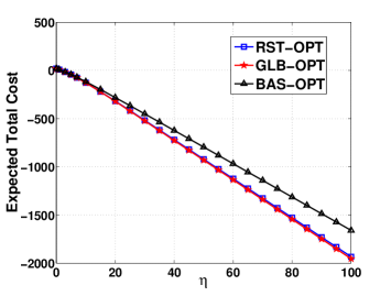
Figure 6: Expected total cost as a function of the trade-off multiplier $\eta$; see (5). Recall that a large $\eta$ implies less emphasis on expected delay.

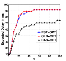
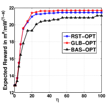
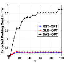
Figure 7: Individual components of the total cost in Fig. 6 as functions of $\eta$: 7 Delay 7 Reward and 7 Probing Cost.

Discussion: In Fig. 6 we have plotted the total cost (i.e., the objective in (5)) incurred by each of the above policies as a function of the multiplier $\eta$. GLB-OPT being the globally optimal policy achieves the minimum cost. However, interestingly we observe that the total cost obtained by RST-OPT is very close to that of GLB-OPT. While the performance of BAS-OPT is good for small values of $\eta$, the performance degrades as $\eta$ increases illustrating that it is not wise to naively probe every relay as and when they wake-up.

In Fig. 7 we have shown the individual components of the total cost (namely delay, reward, and probing cost) as functions of $\eta$. As $\eta$ decreases to $0$ we see (from Fig. 7) that the expected delay incurred by all the policies converges to $20$ ms which is the mean time, $\tau$, until the first relay wakes up. Similarly, the expected rewards (in Fig. 7) converge to reward of the first relay, and the probing costs (in Fig. 7) converge to the cost of probing a single relay, i.e., $\delta=1$ mW. This is because, for small values of $\eta$, since delay is valued more (recall the total cost expression from (5)), all the policies essentially end up probing the first relay and then forwarding the packet to it. This also explains as to why similar total cost (recall Fig. 6) is incurred by all the policies in the low $\eta$ regime (e.g., $\eta\leq 20$).

Next, as $\eta$ increases we see that the delay incurred and the reward achieved by all the policies increases (see Fig. 7 and 7, respectively). While the probing cost of BAS-OPT naively increases (see Fig. 7), probing costs incurred by RST-OPT and GLB-OPT saturate beyond $\eta=20$. This is because, whenever $\eta$ is large, RST-OPT and GLB-OPT are aware that the gain in reward value obtained by probing more relays is negated by the cost term, $\eta\delta$, which is added to the total cost each time a new relay is probed; BAS-OPT, not allowed to not-probe, ends up probing all the relays until the best reward exceeds the threshold $\alpha$. Thus, although BAS-OPT incurs a smaller delay than the other two policies, but suffers both in terms of reward and probing cost, leading to an higher total cost. On the other hand, RST-OPT and GLB-OPT wait for more relays and then probe only the relays with good reward distribution to accrue a better total cost.

Finally, the marginal improvement in performance obtained by GLB-OPT over RST-OPT can be understood as follows. Although the delay incurred by these two policies is almost identical, for large $\eta$ values, GLB-OPT achieves a better reward than RST-OPT by incurring a slightly higher probing cost. Thus, whenever the reward offered by the relay with the best distribution is not good enough, GLB-OPT probes an additional relay to improve the reward; such improvement is not possible by RST-OPT since it is restricted to keep only one unprobed relay awake.

Computational Complexity: Finally on the computational complexity of these policies. To obtain GLB-OPT we had to recursively solve the Bellman equation (referred to as the value iteration) in (24), (25) and (27), for every stage $k$ and every possible state at stage $k$. The total number of all possible states at stage $k$, i.e., the cardinality of the state space $\mathcal{X}_{k}$ in (26), grows exponentially with the cardinality of $\mathcal{F}$ (assuming that $\mathcal{F}$ is discrete like in our numerical example). It also grows exponentially with the stage index $k$.

In contrast, for computing RST-OPT, since within the restricted class at any time only one unprobed relay is kept awake, the state space size grows only linearly with the cardinality of $\mathcal{F}$. Also, the size of the state space does not grow with $k$. Furthermore, from our analysis in Section IV we know that the stopping sets are threshold based, and moreover the thresholds, $\alpha_{k}$ and $\{\alpha_{k}^{\ell}:F_{\ell}\in\mathcal{F}\}$, are stage independent. Hence, these thresholds have to be computed only once (for stage $N-1$ and $N$, respectively), thus further reducing the complexity of RST-OPT. BAS-OPT, being a single-threshold based policy, is much simpler to implement but is not a good choice whenever $\eta$ is large.

VI-B End-to-End Study

The good one-hop performance of RST-OPT and its computational simplicity motivates us to apply RST-OPT to route packets in an asynchronously sleep-wake cycling WSN and study its end-to-end performance. We will also obtain the end-to-end performance of the naive BAS-OPT policy.

First we will describe the setting that we have considered for our end-to-end simulation study. We construct a network by randomly placing $500$ nodes in a square region of side $500$ m. The sink node is placed at the location $(500,0)$. The network nodes are asynchronously and periodically sleep-wake cycling, i.e., a node $i$ wakes up at the periodic instants, $\{T_{i}+kT:k\geq 0\}$, where $\{T_{i}\}$ are i.i.d. uniform on $[0,T]$ with $T$ being the sleep-wake cycling period (recall our justification for the periodic sleep-wake cycling from footnote 1 in page 1). We fix $T=100$ ms. A source node is randomly chosen, which generates an alarm packet at time $0$. This alarm packet has to be routed to the sink node.

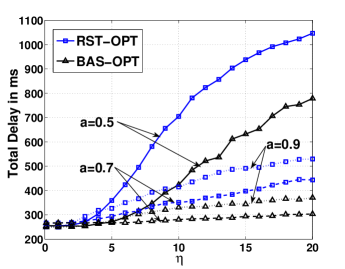
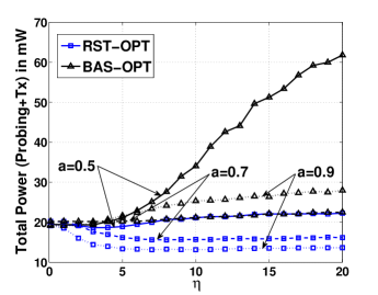
Figure 8: End-to-end performance of RST-OPT and BAS-OPT as functions of $\eta$ for different values of $a$: 8 Total delay, and 8 Total power.

Here, in addition to varying $\eta$, we will also vary the multiplier $a$ and study the end-to-end performance. Recall from (3) that $a$ is the multiplier used to trade-off between progress and power in the reward expression; a larger value of $a$ implies more emphasis on progress. The values of all the other parameters, e.g., $r_{c}$, $\delta$, $\Gamma N_{0}$, channel gains, etc., remain as in our one-hop study.

Now, for a given $\eta$ and $a$, each node computes the corresponding RST-OPT and BAS-OPT policies assuming a mean inter-wake-up time of $\frac{T}{N_{i}}$ ms, where $N_{i}$ is the number of nodes in the forwarding region of node $i$. In Fig. 8, for three different values of $a$ (namely $0.5$, $0.7$, and $0.9$) we have plotted, as functions of $\eta$, the total delay and the total power (which is the sum of the probing and the transmission powers incurred at each hop) incurred, by applying RST-OPT and BAS-OPT policies at each hop en-route to the sink node. Each data point in Fig. 8 is obtained by averaging the respective quantities over $1000$ alarm packets.

Discussion: First, note that both total delay and total power incurred by BAS-OPT are increasing with $\eta$ for each $a$. Hence, no favorable trade-off between delay and power can be obtained using BAS-OPT; it is better to operate BAS-OPT at a low value of $\eta$, where the total delay incurred is (approximately) 250 ms while the total power expended is about 20 mW. In fact, as $\eta$ decreases to $0$, we see that the performance of all the policies (i.e., RST-OPT and BAS-OPT for different values of $a$) converge to these values. This is simply because, whenever $\eta$ is small, since (one-hop) delay is valued more, all the policies, at each hop, essentially forward the packet to the first relay that wakes up.

For RST-OPT, while only a marginal trade-off between delay and power can be achieved for $a=0.5$ (see from Fig. 8 that the corresponding total power decreases only marginally as $\eta$ increases from $1$ to $4$), but as we increase the value of $a$ to $0.7$ and then to $0.9$, we see that the total power sharply decreases with $\eta$. For instance, for $a=0.9$, from Fig. 8 we see that the total power decrease from $20$ mW to $13$ mW as $\eta$ goes from $0$ to $7$. However, over this range of $\eta$, total delay increases from $250$ ms to $360$ ms (see the plot corresponding to RST-OPT, $a=0.9$, from Fig. 8). Thus, for these higher values of $a$, trade-off between delay and power can be achieved using RST-OPT.

Next, for any fixed $\eta$, from Fig. 8 observe that the total power incurred by RST-OPT is improving (i.e., decreasing) with $a$. This can be understood as follows: since a larger $a$ gives less emphasis on power and more emphasis on progress in the reward expression (recall (3)), then, although the one-hop transmissions may be of higher power, but there are fewer hops and hence fewer transmissions, thus resulting in a lower total power. This observation would suggest that it is advantageous to use RST-OPT by setting $a=0.9$ rather than $a=0.5$ or $0.7$. However, from Fig. 8 we see that the total delay is not decreasing with $a$. In fact, delay incurred by RST-OPT first decreases as $a$ increases from $0.5$ to $0.7$, and then increases as $a$ is further increased to $0.9$. Similar is the case for the plots corresponding to BAS-OPT in Fig. 8. This observation can be understood as follows. When $a=0.5$, since (one-hop) power is valued more, the respective forwarding nodes at each hop will end up spending more time waiting for a relay which require strictly lesser transmission power. Similarly, when $a=0.9$, larger delay is incurred at each hop since the forwarding nodes now have to wait for relays whose progress value is more (however, since $a=0.9$ results in a fewer hops we see that the delay incurred in this case is considerably less than the $a=0.5$ case). On the other hand, when $a=0.7$, since a relatively fair trade-off between progress and power exists, the waiting time at each hop is reduced because now any relay with a moderate progress and a moderate transmission power would suffice.

The above argument is precisely the reason as to why the total power incurred by BAS-OPT behaves as in Fig. 8: when $a=0.5$ or $0.9$, each forwarder, in the process of waiting for a relay whose transmission power requirement is low or progress is large, respectively, will end up probing more relays. RST-OPT benefits over BAS-OPT here by probing only good relays at each hop, thus yielding a lower total power.

Finally, summarizing our end-to-end results, we see that no trade-off between delay and power can be achieved by the naive BAS-OPT policy, while RST-OPT achieves such a trade-off (by varying $\eta$) for $a=0.7$ or $0.9$. Further, for a fixed $\eta$, favorable trade-off between delay and power can be obtained by varying $a$. For instance, from Fig. 8 we see that when $\eta=7$, moving from $a=0.7$ to $0.9$ will result in a power saving of about $3$ mW while increasing the end-to-end delay by $130$ ms. Thus, depending on the application requirement (i.e., delay or power sensitive application) one has to appropriately choose the values of $\eta$ and $a$.

VII Conclusion

Motivated by the problem of end-to-end geographical forwarding in a sleep-wake cycling wireless sensor network, we formulated a decision problem of choosing a next-hop relay node when a set of potential relay neighbors are sequentially waking up in time. A power cost is incurred for probing a relay to learn its channel gain. We first studied a restricted class of policies where a policy’s decision is based only on, in addition to the best probed relay, the best unprobed relays (instead of all the unprobed relays). We characterized the optimal policy in terms of stopping sets. Our first main result (Theorem 1) was to show that the stopping sets are threshold based. Then we proved that the stopping sets are stage independent (Theorem 2 and 3). A discussion on the more general unrestricted class of policies was provided. We conducted numerical work to compare the performances of the restricted optimal (RST-OPT) and the global optimal (GLB-OPT) policies. We observed that the performance of RST-OPT is close to that of GLB-OPT. We also conducted simulation experiments to study the end-to-end performance of RST-OPT. Finally, it is worth noting that our work being a variant of the asset selling problem, can, in general, find application wherever the problem of resource-selection occurs, when a collection of resources are sequentially arriving.

Appendix A Proof of Lemma 2

For convenience, here in the appendix, we will recall the respective Lemma/Theorem statements before providing their proofs. Now, before proceeding to the proof of Lemma 2, we will require the following result first.

Lemma 8

For $k=1,2,\cdots,N$, $J_{k}(b)$ and $J_{k}(b,F_{\ell})$ are decreasing in $b$.

Proof:

Proof is by induction. For stage $N$ we know that $J_{N}(b)=-\eta b$, and hence is decreasing in $b$. Also, recalling $J_{N}(b,F_{\ell})$ from (11):

$$J_{N}(b,F_{\ell})=\min\Big{\{}-\eta b,\eta\delta-\eta\mathbb{E}_{\ell}\Big{[}\max\{b,R_{\ell}\}\Big{]}\Big{\}},$$

it is easy to see that $J_{N}(b,F_{\ell})$ is also decreasing in $b$. Thus, the monotonicity properties holds for stage $N$. Now, suppose $J_{k+1}(b)$ and $J_{k+1}(b,F_{\ell})$ (for all $F_{\ell}$) are decreasing in $b$ for some $k+1=2,3,\cdots,N$, then we will show that the result holds for stage $k$ as well.

First, recall the expressions of $J_{k}(b)$ and $J_{k}(b,F_{\ell})$ (from (17) and (18) respectively): $J_{k}(b)=\min\Big{\{}-\eta b,C_{k}(b)\Big{\}}$ and $J_{k}(b,F_{\ell})=\min\Big{\{}-\eta b,P_{k}(b,F_{\ell}),C_{k}(b,F_{\ell})\Big{\}}$. Thus to complete the proof it is sufficient to show that $C_{k}(b)$, $P_{k}(b,F_{\ell})$ and $C_{k}(b,F_{\ell})$ are decreasing in $b$. From the induction hypothesis, it is easy to see that $C_{k}(b)$ (in (14)) is decreasing in $b$, so that we obtain $J_{k}(b)$ is decreasing in $b$. Now that we have established $J_{k}(b)$ is decreasing in $b$, it will immediately follow that the probing cost $P_{k}(b,F_{\ell})$ (in (16)) is decreasing in $b$. Finally, again using the induction argument, observe that $\min\Big{\{}J_{k+1}(b,F_{\ell}),J_{k+1}(b,F_{L_{k+1}})\Big{\}}$ is decreasing in $b$ so that the continuing cost $C_{k}(b,F_{\ell})$ (in (15)) is also decreasing. ∎

We are now ready to prove Lemma 2.

Lemma 2:

1. For $k=1,2,\cdots,N-1$, if $F_{\ell}\geq_{st}F_{u}$ then $C_{k}(b,F_{\ell})\leq C_{k}(b,F_{u})$, (including $k=N$) $P_{k}(b,F_{\ell})\leq P_{k}(b,F_{u})$ and $J_{k}(b,F_{\ell})\leq J_{k}(b,F_{u})$.

2. For $k=1,2,\cdots,N-2$, $C_{k}(b)\leq C_{k+1}(b)$ and $C_{k}(b,F_{\ell})\leq C_{k+1}(b,F_{\ell})$, (including $k=N-1$) $P_{k}(b,F_{\ell})\leq P_{k+1}(b,F_{\ell})$ and $J_{k}(b,F_{\ell})\leq J_{k+1}(b,F_{\ell})$.

Proof:

Consider stage $N$ and recall the expression for the optimal cost-to-go function $J_{N}(b,F_{\ell})$ from (11):

$$J_{N}(b,F_{\ell}) = \min\Big{\{}-\eta b,P_{N}(b,F_{\ell})\Big{\}}$$

$$= \min\Big{\{}-\eta b,\eta\delta-\eta\mathbb{E}_{\ell}\Big{[}\max\{b,R_{\ell}\}\Big{]}\Big{\}}.$$

Since the function $f(r)=\max\{b,r\}$ is increasing in $r$, using the definition of stochastic ordering (Definition 2) we can write

$$\mathbb{E}_{\ell}\Big{[}\max\{b,R_{\ell}\}\Big{]}\geq\mathbb{E}_{u}\Big{[}\max\{b,R_{u}\}\Big{]},$$

so that we have $P_{N}(b,F_{\ell})\leq P_{N}(b,F_{u})$ and $J_{N}(b,F_{\ell})\leq J_{N}(b,F_{u})$. Thus, the result holds for stage $N$.

Now suppose the result is true for some $k+1=2,3,\cdots,N$. From Lemma 8 we know that $J_{k}(b)$ is decreasing in $b$, which would imply that, for any $b$, the function $f(r)=J_{k}(\max\{b,r\}))$ is decreasing in $r$. Again, using the definition of stochastic ordering (in Definition 2) we can conclude that

$$\mathbb{E}_{\ell}\Big{[}J_{k}(\max\{b,R_{\ell}\})\Big{]}\leq\mathbb{E}_{u}\Big{[}J_{k}(\max\{b,R_{u}\})\Big{]},$$

so that $P_{k}(b,F_{\ell})\leq P_{k}(b,F_{u})$ (see (16)). Next, from the induction argument we know that $J_{k+1}(b,F_{\ell})\leq J_{k+1}(b,F_{u})$ so that

$$\min\Big{\{}J_{k+1}(b,F_{\ell}),J_{k+1}(b,F_{L_{k+1}})\Big{\}}\leq\min\Big{\{}J_{k+1}(b,F_{u}),J_{k+1}(b,F_{L_{k+1}})\Big{\}}.$$

Therefore, we also have $C_{k}(b,F_{\ell})\leq C_{k}(b,F_{u})$ (see (15)). The proof can now be easily completed by recalling (from (18)) that $J_{k}(b,F_{\ell})=\min\Big{\{}-\eta b,P_{k}(b,F_{\ell}),C_{k}(b,F_{\ell})\Big{\}}$.

Proof of Part-(ii): This result is very intuitive, since with more number of stages to go, one is expected to accrue a lower cost. However, we prove it here for completeness. Again the proof is by induction. For stage $N-1$ we easily have,

$$J_{N-1}(b) = \min\Big{\{}-\eta b,C_{k}(b)\Big{\}}$$

$$\leq -\eta b$$

$$= J_{N}(b).$$

Next, consider a state of the form $(b,F_{\ell})$. The cost of probing $P_{N-1}(b,F_{\ell})$ can be bounded as follows:

$$P_{N-1}(b,F_{\ell}) = \eta\delta+\mathbb{E}_{\ell}\Big{[}J_{N-1}(\max\{b,R_{\ell}\})\Big{]}$$

$$\overset{*}{\leq} \eta\delta+\mathbb{E}_{\ell}\Big{[}J_{N}(\max\{b,R_{\ell}\})\Big{]}$$

$$\overset{o}{=} \eta\delta-\eta\mathbb{E}_{\ell}\Big{[}\max\{b,R_{\ell}\}\Big{]}$$

$$\overset{\dagger}{=} P_{N}(b,F_{\ell}),$$

where, to obtain $*$ we have used, $J_{N-1}(b)\leq J_{N}(b)$ (which we had just proved), $o$ is because $J_{N}(b)=-\eta b$ for all $b$, and $\dagger$ is simply obtained by recalling the expression for $P_{N}(b,F_{\ell})$. Using the above inequality in the following, we obtain

$$J_{N-1}(b,F_{\ell}) = \min\Big{\{}-\eta b,P_{N-1}(b,F_{\ell}),C_{N-1}(b,F_{\ell})\Big{\}}$$

$$\leq \min\Big{\{}-\eta b,P_{N-1}(b,F_{\ell})\Big{\}}$$

$$\leq \min\Big{\{}-\eta b,\eta\delta-\eta\mathbb{E}_{\ell}\Big{[}\max\{b,R_{\ell}\}\Big{]}\Big{\}}$$

$$= J_{N}(b,F_{\ell}).$$

Thus we have shown the result for stage $N-1$.

Suppose the result is true for some stage $k+1=2,3,\cdots,N-1$. i.e., $J_{k+1}(b)\leq J_{k+2}(b)$ and $J_{k+1}(b,F_{\ell})\leq J_{k+2}(b,F_{\ell})$ (for all $F_{\ell}$), then, using the induction hypothesis, the cost of continuing, $C_{k}(b)$, can be bounded as

$$C_{k}(b) = \tau+\mathbb{E}_{L}\Big{[}J_{k+1}(b,F_{k+1})\Big{]}$$

$$\leq \tau+\mathbb{E}_{L}\Big{[}J_{k+2}(b,F_{k+2})\Big{]}$$

$$= C_{k+1}(b).$$

Thus, we have $J_{k}(b)\leq J_{k+1}(b)$ (see (17)). Next, consider the probing cost,

$$P_{k}(b,F_{\ell}) = \eta\delta+\mathbb{E}_{\ell}\Big{[}J_{k}(\max\{b,R_{\ell}\})\Big{]}$$

$$\overset{*}{\leq} \eta\delta+\mathbb{E}_{\ell}\Big{[}J_{k+1}(\max\{b,R_{\ell}\})\Big{]}$$

$$= P_{k+1}(b,F_{\ell})$$

where, to obtain $*$ we have used $J_{k}(b)\leq J_{k+1}(b)$ which we have already shown. The cost of continuing can be similarly bounded:

$$C_{k}(b,F_{\ell}) = \tau+\mathbb{E}_{L}\Big{[}\min\{J_{k+1}(b,F_{\ell}),J_{k+1}(b,F_{L_{k+1}})\}\Big{]}$$

$$\overset{*}{\leq} \tau+\mathbb{E}_{L}\Big{[}\min\{J_{k+2}(b,F_{\ell}),J_{k+2}(b,F_{L_{k+2}})\}\Big{]}$$

$$= C_{k+1}(b,F_{\ell}),$$

where $*$ is due to the induction hypothesis and the fact that location random variables, $L_{k+1}$ and $L_{k+2}$, are identically distributed. Finally, using the above inequalities in the expression of $J_{k}(b,F_{\ell})$ (recall (18); $J_{k}(b,F_{\ell})=\min\Big{\{}-\eta b,P_{k}(b,F_{\ell}),C_{k}(b,F_{\ell})\Big{\}}$), we obtain $J_{k}(b,F_{\ell})\leq J_{k+1}(b,F_{\ell})$, thus completing the proof. ∎

Appendix B Proof of Lemma 4

The following simple property about the $\min$-operator will be useful while proving Lemma 4.

Lemma 9

If $x_{1},x_{2},\cdots,x_{j}$ and $y_{1},y_{2},\cdots,y_{j}$ in $\Re$, are such that, $x_{i}-y_{i}\leq x_{1}-y_{1}$ for all $i=1,2,\cdots,j$, then

$$\min\{x_{1},x_{2},\cdots,x_{j}\}-\min\{y_{1},y_{2},\cdots,y_{j}\}\leq x_{1}-y_{1}$$ (28)

Proof:

Suppose $\min\{y_{1},y_{2},\cdots,y_{j}\}=y_{i}$, for some $1\leq i\leq j$, then the LHS of (28) can be written as,

$$LHS=\min\{x_{1},x_{2},\cdots,x_{j}\}-y_{i}\leq x_{i}-y_{i}.$$

The proof is complete by recalling that we are given, $x_{i}-y_{i}\leq x_{1}-y_{1}$. ∎

Lemma 4: For $k=1,2,\cdots,N-1$ (for part (ii), $k=1,2,\cdots,N$), for any $F_{\ell}$, and for $b_{2}>b_{1}$ we have

1. $C_{k}(b_{1})-C_{k}(b_{2})\leq\eta(b_{2}-b_{1})$,

2. $P_{k}(b_{1},F_{\ell})-P_{k}(b_{2},F_{\ell})\leq\eta(b_{2}-b_{1})$

3. $C_{k}(b_{1},F_{\ell})-C_{k}(b_{2},F_{\ell})\leq\eta(b_{2}-b_{1})$.

Proof:

Since $J_{N}(b)$ is $-\eta b$ we already have, for stage $N$, $J_{N}(b_{1})-J_{N}(b_{2})=\eta(b_{2}-b_{1})$. Also, for a given distribution $F_{\ell}$ and for $b_{2}>b_{1}$,

$$P_{N}(b_{1},F_{\ell})-P_{N}(b_{2},F_{\ell}) = \eta\mathbb{E}_{\ell}\Big{[}\max\{b_{2},R_{\ell}\}-\max\{b_{1},R_{\ell}\}\Big{]}$$

$$\overset{*}{\leq} \eta(b_{2}-b_{1}),$$

where to obtain $*$, first consider all the three cases that are possible: (1) $R_{\ell}\leq b_{1}<b_{2}$, (2) $b_{1}<R_{\ell}<b_{2}$, and (3) $b_{1}<b_{2}\leq R_{\ell}$, and then note that in all these cases, $\Big{(}\max\{b_{2},R_{\ell}\}-\max\{b_{1},R_{\ell}\}\Big{)}$, is bounded above by $b_{2}-b_{1}$. Now, since $J_{N}(b,F_{\ell})=\min\Big{\{}-\eta b,P_{N}(b,F_{\ell})\Big{\}}$, the above inequality along with Lemma 9 will yield, $J_{N}(b_{1},F_{\ell})-J_{N}(b_{2},F_{\ell})\leq\eta(b_{2}-b_{1})$.

Suppose for some stage $k+1=1,2,\cdots,N$ we have $J_{k+1}(b_{1})-J_{k+1}(b_{2})\leq\eta(b_{2}-b_{1})$ and $J_{k+1}(b_{1},F_{\ell})-J_{k+1}(b_{2},F_{\ell})\leq\eta(b_{2}-b_{1})$ for all $b_{2}>b_{1}$, and for all $F_{\ell}$. Then we will show that all the inequalities listed in the lemma will hold for stage $k$ as well. First, a simple application of the induction hypothesis will yield,

$$C_{k}(b_{1})-C_{k}(b_{2}) = \mathbb{E}_{L}\Big{[}J_{k+1}(b_{1},F_{L_{k}})-J_{k+1}(b_{2},F_{L_{k}})\Big{]}$$

$$\leq \eta(b_{2}-b_{1}).$$

Since $J_{k}(b)=\min\Big{\{}-\eta b,C_{k}(b)\Big{\}}$, the above inequality along with Lemma 9 gives, $J_{k}(b_{1})-J_{k}(b_{2})\leq\eta(b_{2}-b_{1})$, for any $b_{2}>b_{1}$. Using this we can write

$$P_{k}(b_{1},F_{\ell})-P_{k}(b_{2},F_{\ell}) = \mathbb{E}_{\ell}\Big{[}J_{k}(\max\{b_{1},R_{\ell}\})-J_{k}(\max\{b_{2},R_{\ell}\})\Big{]}$$ (29)

$$\leq \mathbb{E}_{\ell}\Big{[}\eta\Big{(}\max\{b_{2},R_{\ell}\}-\max\{b_{1},R_{\ell}\}\Big{)}\Big{]}$$

$$\leq \eta(b_{2}-b_{1}),$$

where the last inequality is again by considering all the three regions where $R_{\ell}$ can lie.

To show part (iii), define $\mathcal{L}_{\ell}$ as the set of all distributions that are stochastically greater than $\ell$, i.e., $\mathcal{L}_{\ell}=\Big{\{}F_{t}\in\mathcal{F}:F_{t}\geq_{st}F_{\ell}\Big{\}}$. Let $\mathcal{L}_{\ell}^{c}$ denote the set of all the remaining distributions, i.e., $\mathcal{L}_{\ell}^{c}=\mathcal{F}\setminus\mathcal{L}_{\ell}$. From Lemma 5, where we have shown that $\mathcal{F}$ is totally stochastically ordered (see Definition 3), it follows that $\mathcal{L}_{\ell}^{c}$ contains all distributions in $\mathcal{F}$ which are stochastically smaller than $F_{\ell}$. Recalling the expression for $C_{k}(b,F_{\ell})$ from (15), the difference in the cost of continuing can now be bounded as follows:

$$C_{k}(b_{1},F_{\ell})-C_{k}(b_{2},F_{\ell}) = \int_{\mathcal{F}}\Big{(}\min\{J_{k+1}(b_{1},F_{\ell}),J_{k+1}(b_{1},F_{t})\}$$ (30)

$$\hskip 56.9055pt-\min\{J_{k+1}(b_{2},F_{\ell}),J_{k+1}(b_{2},F_{t})\}\Big{)}dL(t)$$

$$\overset{*}{=} \int_{\mathcal{L}_{\ell}}(J_{k+1}(b_{1},F_{t})-J_{k+1}(b_{2},F_{t}))dL(t)$$

$$\hskip 56.9055pt+\int_{\mathcal{L}_{\ell}^{c}}(J_{k+1}(b_{1},F_{\ell})-J_{k+1}(b_{2},F_{\ell}))dL(t).$$

$$\overset{o}{\leq} \eta(b_{2}-b_{1}).$$

In the above derivation, $*$ is obtained by using Lemma 2-(i), and $o$ is simply by applying the induction argument. Since $J_{k}(b,F_{\ell})=\min\Big{\{}-\eta b,P_{k}(b,F_{\ell}),C_{k}(b,F_{\ell})\Big{\}}$, using (29) and (30) along with Lemma 9, we obtain, $J_{k}(b_{1},F_{\ell})-J_{k}(b_{2},F_{\ell})\leq\eta(b_{2}-b_{1})$, thus completing the induction argument. ∎

Appendix C Proof of Lemma 5

Lemma 5: The set of reward distributions $\mathcal{F}$ in (4), is totally stochastically ordered with a minimum distribution.

Proof:

Recall the reward expression from (3),

$$R_{\ell}=\frac{Z_{\ell}^{a}}{P_{\ell}^{(1-a)}}=\frac{Z_{\ell}^{a}}{(\Gamma^{\prime}D_{\ell}^{\xi})^{(1-a)}}G_{\ell}^{(1-a)}.$$

The distribution, $F_{\ell}$, of $R_{\ell}$ can be written as,

$$F_{\ell}(r) = \mathbb{P}(R_{\ell}\leq r)$$ (31)

$$= \mathbb{P}\left(\frac{Z_{\ell}^{a}}{(\Gamma^{\prime}D_{\ell}^{\xi})^{(1-a)}}G_{\ell}^{(1-a)}\leq r\right)$$

$$= \mathbb{P}\left(G_{\ell}^{(1-a)}\leq{\kappa}_{\ell}r\right),$$

where $\kappa_{\ell}=\frac{(\Gamma^{\prime}D_{\ell}^{\xi})^{(1-a)}}{Z_{\ell}^{a}}$.

Let $\ell,u$ be any two locations in $\mathcal{L}$. Since the rewards are non-negative, we have $F_{\ell}(r)=F_{u}(r)=0$ for $r<0$. Hence, we only need to consider the case $r\geq 0$. Now, given $\ell,u\in\mathcal{L}$, either $\kappa_{\ell}\leq\kappa_{u}$ or $\kappa_{\ell}>\kappa_{u}$. Thus we have, either $\kappa_{\ell}r\leq\kappa_{u}r$ or $\kappa_{\ell}r\geq\kappa_{u}r$, for every $r\geq 0$. Finally, since $G_{\ell}$ and $G_{u}$ are identically distributed, we have, either $F_{\ell}(r)\leq F_{u}(r)$ or $F_{\ell}(r)\geq F_{u}(r)$, for all $r$, so that $F_{\ell}$ and $F_{u}$ are stochastically ordered (recall Definition 2).

To show that there exists a minimum distribution, first note that $\kappa_{\ell}$ as a function of $\ell\in\mathcal{L}$ is continuous. Then, since we had assumed that $\mathcal{L}$ is compact (closed and bounded), there exists an $m\in\mathcal{L}$ where the maximum is achieved, i.e., $\kappa_{\ell}\leq\kappa_{m}$ for all $\ell\in\mathcal{L}$. Again, since the gains $G_{\ell}$ and $G_{m}$ are identically distributed, from (31) it follows that $F_{\ell}\geq_{st}F_{m}$ for all $\ell\in\mathcal{L}$, so that $F_{m}$ is the minimum distribution. ∎

Appendix D Proof of Lemma 6

Lemma 6: Suppose $\mathcal{S}_{k}\subseteq\mathcal{Q}_{k}^{u}$, for some $F_{u}$, and some $k=1,2,\cdots,N-1$. Then for every $b\in\mathcal{S}_{k}$ we have $J_{k}(b,F_{u})=J_{N}(b,F_{u})$.

Proof:

Fix a $b\in\mathcal{S}_{k}\subseteq\mathcal{Q}_{k}^{u}$. Then,

$$J_{k}(b,F_{u}) = \min\Big{\{}-\eta b,P_{k}(b,F_{u}),C_{k}(b,F_{u})\Big{\}}$$

$$\overset{*}{=} \min\Big{\{}-\eta b,P_{k}(b,F_{u})\Big{\}}$$

$$\overset{o}{=} \min\Big{\{}-\eta b,\eta\delta+\mathbb{E}_{u}\Big{[}J_{k}(\max\{b,R_{u}\})\Big{]}\Big{\}}$$

$$\overset{\dagger}{=} \min\Big{\{}-\eta b,\eta\delta-\eta\mathbb{E}_{u}\Big{[}\max\{b,R_{u}\}\Big{]}\Big{\}}$$

$$= J_{N}(b,F_{u}).$$

In the above derivation, $*$ is because, $b$ being in $\mathcal{Q}_{k}^{u}$, at $(b,F_{u})$ it is optimal to either stop or probe (recall (22)). $o$ is simply obtained by substituting for $P_{k}(b,F_{u})$ from (16). Further, after probing the new state, $\max\{b,R_{u}\}\geq b$, is also in $\mathcal{S}_{k}$ (from Theorem 1) so that it is optimal to stop after probing. This observation yields $\dagger$. Finally, the last equality is obtained by recalling the expression of $J_{N}(b,F_{u})$ from (11). ∎

Appendix E Proof of Lemma 7

As discussed in the outline of the proof of Lemma 7, the result immediately follows once we show Step 1 and Step 2. First we will formally state and prove Step 1.

Lemma 10

Suppose $F_{u}$ is a distribution such that for all $k=1,2,\cdots,N-1$, $\mathcal{S}_{k}\subseteq\mathcal{Q}_{k}^{u}$. Then for any distribution $F_{\ell}\geq_{st}F_{u}$ we have $\mathcal{S}_{k}\subseteq\mathcal{Q}_{k}^{\ell}$.

Proof:

We will first show that $\mathcal{S}_{N-1}\subseteq\mathcal{Q}_{N-1}^{\ell}$. Fix a $b\in\mathcal{S}_{N-1}$. Then $b\in\mathcal{Q}_{N-1}^{u}$ (because it is given that $\mathcal{S}_{N-1}\subseteq\mathcal{Q}_{N-1}^{u}$), so that using the definition of the set $\mathcal{Q}_{N-1}^{u}$ (from (22)) we can write

$$\min\Big{\{}-\eta b,P_{N-1}(b,F_{u})\Big{\}}\leq C_{N-1}(b,F_{u}).$$ (32)

For any generic distribution $F_{s}$, whenever $b\in\mathcal{S}_{N-1}$, the minimum of the cost of stopping and the cost of probing can be simplified as follows:

$$\min\Big{\{}-\eta b,P_{N-1}(b,F_{s})\Big{\}} \overset{*}{=} \min\Big{\{}-\eta b,\eta\delta+\mathbb{E}_{s}\Big{[}J_{N-1}(\max\{b,R_{s}\})\Big{]}\Big{\}}$$ (33)

$$\overset{o}{=} \min\Big{\{}-\eta b,\eta\delta-\eta\mathbb{E}_{s}\Big{[}\max\{b,R_{s}\}\Big{]}\Big{\}}$$

$$\overset{\dagger}{=} J_{N}(b,F_{s}).$$

In the above, $*$ is obtained by recalling the expression for the probing cost from (16). $o$ is because, after probing we are still at stage $N-1$ with the new state $\max\{b,R_{s}\}$ also in $\mathcal{S}_{N-1}$ (Lemma 1); in $\mathcal{S}_{N-1}$ we know that it is optimal to stop, so that $J_{N-1}(\max\{b,R_{s}\})=-\eta\max\{b,R_{s}\}$. Finally, to obtain $\dagger$, recall the expression for $J_{N}(b,F_{s})$ from (11).

Now using (33) in (32) we see that, the hypothesis $b\in\mathcal{S}_{N-1}$ implies, $J_{N}(b,F_{u})\leq C_{N-1}(b,F_{u})$. Also, from Lemma 2-(i) we have, $J_{N}(b,F_{\ell})\leq J_{N}(b,F_{u})$ for any $F_{\ell}\geq_{st}F_{u}$. Combining these we can write

$$J_{N}(b,F_{\ell})\leq J_{N}(b,F_{u})\leq C_{N-1}(b,F_{u}).$$ (34)

To conclude that $b\in\mathcal{Q}_{N-1}^{\ell}$, we need to show

$$\min\Big{\{}-\eta b,P_{N-1}(b,F_{\ell})\Big{\}}\leq C_{N-1}(b,F_{\ell}),$$

or, alternatively, recalling (33), it is sufficient to show,

$$J_{N}(b,F_{\ell})\leq C_{N-1}(b,F_{\ell}).$$ (35)

Now for any generic distribution $F_{s}\in\mathcal{F}$ define $\mathcal{L}_{s}=\Big{\{}t\in\mathcal{L}:F_{t}\geq_{st}F_{s}\Big{\}}$ i.e., $\mathcal{L}_{s}$ is the set of all distributions in $\mathcal{F}$ that are stochastically greater than $F_{s}$. Let $\mathcal{L}_{\ell}^{c}$ denote the set of all the remaining distributions, i.e., $\mathcal{L}_{\ell}^{c}=\mathcal{F}\setminus\mathcal{L}_{\ell}$. Since $\mathcal{F}$ is totally stochastically ordered (Lemma 5), $\mathcal{L}_{s}^{c}$ contains all distributions in $\mathcal{F}$ that are stochastically smaller than $F_{s}$. Further, for $F_{\ell}\geq_{st}F_{u}$ we have $\mathcal{L}_{\ell}\subseteq\mathcal{L}_{u}$. Then, recalling the expression for $C_{N-1}(b,F_{u})$ from (15) we can write

$$C_{N-1}(b,F_{u}) = \tau+\mathbb{E}_{L}\Big{[}\min\{J_{N}(b,F_{u}),J_{N}(b,F_{L_{N}})\}\Big{]}$$

$$\overset{*}{=} \tau+\int_{\mathcal{L}_{u}}J_{N}(b,F_{t})\ dL(t)+\int_{\mathcal{L}_{u}^{c}}J_{N}(b,F_{u})\ dL(t)$$

$$\overset{o}{=} \tau+\int_{\mathcal{L}_{\ell}}J_{N}(b,F_{t})\ dL(t)+\int_{\mathcal{L}_{u}\setminus\mathcal{L}_{\ell}}J_{N}(b,F_{t})\ dL(t)+\int_{\mathcal{L}_{u}^{c}}J_{N}(b,F_{u})\ dL(t),$$

where, $*$ is obtained by using Lemma 2-(i) and the definition of $\mathcal{L}_{u}$, and to obtain $o$ we have split the integral over $\mathcal{L}_{u}$ (first integral in $*$) into two integrals $-$ one over $\mathcal{L}_{\ell}$ and the other over $\mathcal{L}_{u}\setminus\mathcal{L}_{\ell}$. Now, for any $F_{t}\in\mathcal{L}_{u}\setminus\mathcal{L}_{\ell}$ we know that $F_{t}\geq_{st}F_{u}$ so that $J_{N}(b,F_{t})\leq J_{N}(b,F_{u})$ (again from Lemma 2-(i)). Thus, in the above expression, replacing $J_{N}(b,F_{t})$ by $J_{N}(b,F_{u})$ in the middle integral, and then combining it with the last integral, we obtain

$$C_{N-1}(b,F_{u}) \leq \tau+\int_{\mathcal{L}_{\ell}}J_{N}(b,F_{t})\ dL(t)+\left(\int_{\mathcal{L}_{\ell}^{c}}dL(t)\right)\ J_{N}(b,F_{u})$$ (36)

From (34) and (36) we see that we have an inequality of the following form

$$J_{N}(b,F_{\ell})\leq J_{N}(b,F_{u})\leq c+pJ_{N}(b,F_{u}),$$ (37)

where $c=\tau+\int_{\mathcal{L}_{\ell}}J_{N}(b,F_{t})\ dL(t)$ and $p=\int_{\mathcal{L}_{\ell}^{c}}dL(t)$. Since $p\in[0,1]$ we can write

$$J_{N}(b,F_{\ell})(1-p)\leq J_{N}(b,F_{u})(1-p),$$

rearranging which we obtain,

$$J_{N}(b,F_{\ell}) \leq pJ_{N}(b,F_{\ell})+J_{N}(b,F_{u})-pJ_{N}(b,F_{u})$$

$$\overset{*}{\leq} pJ_{N}(b,F_{\ell})+c+pJ_{N}(b,F_{u})-pJ_{N}(b,F_{u})$$

$$= c+pJ_{N}(b,F_{\ell})$$

where, to obtain $*$ we have used (37). Finally, note that

$$c+pJ_{N}(b,F_{\ell}) = \tau+\int_{\mathcal{L}_{\ell}}J_{N}(b,F_{t})\ dL(t)+\left(\int_{\mathcal{L}_{\ell}^{c}}dL(t)\right)J_{N}(b,F_{\ell})$$

$$= \tau+\mathbb{E}_{L}\Big{[}\min\{J_{N}(b,F_{\ell}),J_{N}(b,F_{L_{N}})\}\Big{]}$$

$$= C_{N-1}(b,F_{\ell}).$$

Thus, as desired we have shown $J_{N}(b,F_{\ell})\leq C_{N-1}(b,F_{\ell})$ (recall the discussion leading to (35)).

Suppose that for some $k+1=2,3,\cdots,N-1$ we have $\mathcal{S}_{k+1}\subseteq\mathcal{Q}_{k+1}^{\ell}$. We will have to show that the same holds for stage $k$. Fix any $b\in\mathcal{S}_{k}$, then for any generic distribution $F_{s}$, exactly as in (33) we have

$$\min\Big{\{}-\eta b,P_{k}(b,F_{s})\Big{\}} = \min\Big{\{}-\eta b,\eta\delta+\mathbb{E}_{s}\Big{[}J_{k}(\max\{b,R_{s}\})\Big{]}\Big{\}}$$ (38)

$$= \min\Big{\{}-\eta b,\eta\delta-\eta\mathbb{E}_{s}\Big{[}\max\{b,R_{s}\}\Big{]}\Big{\}}$$

$$= J_{N}(b,F_{s}).$$

Thus the hypothesis $\mathcal{S}_{k}\subseteq\mathcal{Q}_{k}^{u}$ implies $J_{N}(b,F_{u})\leq C_{k}(b,F_{u})$, and to show $\mathcal{S}_{k}\subseteq\mathcal{Q}_{k}^{\ell}$ it is sufficient to obtain $J_{N}(b,F_{\ell})\leq C_{k}(b,F_{\ell})$. Proceeding as before (recall how (36) was obtained) we can write

$$C_{k}(b,F_{u}) \leq \tau+\int_{\mathcal{L}_{\ell}}J_{k+1}(b,F_{t})\ dL(t)+\left(\int_{\mathcal{L}_{\ell}^{c}}dL(t)\right)\ J_{k+1}(b,F_{u}).$$

Now using Lemma 6, we conclude

$$C_{k}(b,F_{u}) \leq \tau+\int_{\mathcal{L}_{\ell}}J_{k+1}(b,F_{t})\ dL(t)+\int_{\mathcal{L}_{\ell}^{c}}dL(t)\ J_{N}(b,F_{u}).$$

Note that the conditions required to apply Lemma 6 hold i.e., $b\in\mathcal{S}_{k+1}$ (since $\mathcal{S}_{k}\subseteq\mathcal{S}_{k+1}$ from Lemma 3-(iii)) and $\mathcal{S}_{k+1}\subseteq\mathcal{Q}_{k+1}^{u}$ (this is given).

Thus, again we have an inequality of the form $J_{N}(b,F_{\ell})\leq J_{N}(b,F_{u})\leq c^{\prime}+pJ_{N}(b,F_{u})$ (where $c^{\prime}=\tau+\int_{\mathcal{L}_{\ell}}J_{k+1}(b,F_{t})\ dL(t)$). As before we can show that $J_{N}(b,F_{\ell})\leq c^{\prime}+pJ_{N}(b,F_{\ell})$. Finally the proof is complete by showing that $c^{\prime}+pJ_{N}(b,F_{\ell})=C_{k}(b,F_{\ell})$ as follows:

$$C_{k}(b,F_{\ell}) = \tau+\int_{\mathcal{L}_{\ell}}J_{k+1}(b,F_{t})\ dL(t)+\int_{\mathcal{L}_{\ell}^{c}}J_{k+1}(b,F_{\ell})\ dL(t)$$ (39)

$$= c^{\prime}+pJ_{N}(b,F_{\ell}),$$

where to replace $J_{k+1}(b,F_{\ell})$ by $J_{N}(b,F_{\ell})$ we have to again apply Lemma 6. However this time $\mathcal{S}_{k+1}\subseteq\mathcal{Q}_{k+1}^{\ell}$, is by the induction hypothesis. ∎

We still require a distribution $F_{u}$ satisfying $\mathcal{S}_{k}\subseteq\mathcal{Q}_{k}^{u}$, for every $k$. The minimum distribution $F_{m}$ turns out to be useful in this context. The following lemma thus constitutes Step 2 of the proof of Lemma 7.

Lemma 11

For every $k=1,2,\cdots,N-1$, the stobing set $\mathcal{Q}_{k}^{m}$ corresponding to the minimum distribution $F_{m}$ satisfies, $\mathcal{S}_{k}\subseteq\mathcal{Q}_{k}^{m}$.

Proof:

First note that the existence of a minimum distribution $F_{m}$ follows from Lemma 5. Now, $F_{m}$ being minimum we have $F_{\ell}\geq_{st}F_{m}$ for all $F_{\ell}$. Then, using Lemma 2-(i) we can write

$$J_{k+1}(b,F_{L_{k+1}})\leq J_{k+1}(b,F_{m}).$$

Using the above expression in (15) and then recalling (14), we obtain $C_{k}(b,F_{m})=C_{k}(b)$. Finally, the result follows from the definition of the sets $\mathcal{Q}_{k}^{m}$ and $\mathcal{S}_{k}$. ∎

Appendix F Proof of Theorem 3

Theorem 3: For $k=1,2,\cdots,N-1$ and for any $F_{\ell}$, $\mathcal{S}_{k}^{\ell}=\mathcal{S}_{k+1}^{\ell}$.

Proof:

Recalling the definition of the set $\mathcal{S}_{k}^{\ell}$ (from (20)), for any $b\in\mathcal{S}_{k+1}^{\ell}$ we have (if $k+1=N$, note that the following expression will not contain the continuing cost),

$$-\eta b\leq\min\Big{\{}P_{k+1}(b,F_{\ell}),C_{k+1}(b,F_{\ell})\Big{\}}.$$

Suppose, as in Theorem 2, we can show that for any $b\in\mathcal{S}_{k+1}^{\ell}$, the various costs at stages $k$ and $k+1$ are same, i.e., $P_{k}(b,F_{\ell})=P_{k+1}(b,F_{\ell})$ and $C_{k}(b,F_{\ell})=C_{k+1}(b,F_{\ell})$, then the above inequality would imply, $\mathcal{S}_{k}^{\ell}\supseteq\mathcal{S}_{k+1}^{\ell}$. The proof is complete by recalling that we already have $\mathcal{S}_{k}^{\ell}\subseteq\mathcal{S}_{k+1}^{\ell}$ (from Lemma 3-(iii)).

Fix a $b\in\mathcal{S}_{k+1}^{\ell}$. To show that $P_{k}(b,F_{\ell})=P_{k+1}(b,F_{\ell})$, first using Lemma 3-(i) and Theorem 2, note that $\mathcal{S}_{k+1}^{\ell}\subseteq\mathcal{S}_{k+1}=\mathcal{S}_{k}$. Since $b\in\mathcal{S}_{k+1}$ the cost of probing is

$$P_{k+1}(b,F_{\ell}) = \eta\delta+\mathbb{E}_{\ell}\Big{[}J_{k+1}(\max\{b,R_{\ell}\})\Big{]}$$

$$= \eta\delta-\eta\mathbb{E}_{\ell}\Big{[}\max\{b,R_{\ell}\}\Big{]}$$

where, to obtain the second equality, note that $\max\{b,R_{\ell}\}\in\mathcal{S}_{k}$ (from Theorem 1) and hence at $\max\{b,R_{\ell}\}$ it is optimal to stop, so that $J_{k+1}(\max\{b,R_{\ell}\})=-\eta\max\{b,R_{\ell}\}$. Similarly, since $b$ is also in $\mathcal{S}_{k}$ the cost of probing at stage $k$, $P_{k}(b,F_{\ell})$, is again $\eta\delta-\eta\mathbb{E}_{\ell}\Big{[}\max\{b,R_{\ell}\}\Big{]}$. Finally, following the same procedure used to show $C_{k}(b)=C_{k+1}(b)$ in Theorem 2, we can obtain $C_{k}(b,F_{\ell})=C_{k+1}(b,F_{\ell})$, thus completing the proof. ∎

References

- [1] J. Kim, X. Lin, and N. Shroff, “Optimal Anycast Technique for Delay-Sensitive Energy-Constrained Asynchronous Sensor Networks,” IEEE/ACM Transactions on Networking, April 2011.
- [2] K. P. Naveen and A. Kumar, “Relay Selection for Geographical Forwarding in Sleep-Wake Cycling Wireless Sensor Networks,” IEEE Transactions on Mobile Computing, vol. 12, no. 3, pp. 475–488, 2013.
- [3] D. P. Bertsekas and J. N. Tsitsiklis, “An Analysis of Stochastic Shortest Path Problems,” Mathematics of Operations Research, vol. 16, 1991.
- [4] K. P. Naveen and A. Kumar, “Tunable Locally-Optimal Geographical Forwarding in Wireless Sensor Networks with Sleep-Wake Cycling Nodes,” in INFOCOM 2010, 29th IEEE Conference on Computer Communications, March 2010.
- [5] T. Rappaport, Wireless Communications: Principles and Practice, 2nd ed. Upper Saddle River, NJ, USA: Prentice Hall PTR, 2001.
- [6] P. S. C. Thejaswi, J. Zhang, M. O. Pun, H. V. Poor, and D. Zheng, “Distributed Opportunistic Scheduling with Two-Level Probing,” IEEE/ACM Transactions on Networking, vol. 18, no. 5, October 2010.
- [7] D. P. Bertsekas, Dynamic Programming and Optimal Control, Vol. I. Athena Scientific, 2005.
- [8] S. Karlin, Stochastic Models and Optimal Policy for Selling an Asset. Stanford University Press, Stanford, 1962.
- [9] K. Akkaya and M. Younis, “A Survey on Routing Protocols for Wireless Sensor Networks,” Ad Hoc Networks, vol. 3, pp. 325–349, 2005.
- [10] M. Zorzi and R. R. Rao, “Geographic Random Forwarding (GeRaF) for Ad Hoc and Sensor Networks: Multihop Performance,” IEEE Transactions on Mobile Computing, vol. 2, pp. 337–348, 2003.
- [11] E. Cinlar, Introduction to Stochastic Processes. Prentice-Hall, 1975.
- [12] A. Kumar, D. Manjunath, and J. Kuri, Wireless Networking. San Francisco, CA, USA: Morgan Kaufmann Publishers Inc., 2008.
- [13] P. Agrawal and N. Patwari, “Correlated Link Shadow Fading in Multi-Hop Wireless Networks,” IEEE Transactions on Wireless Communications, vol. 8, no. 8, pp. 4024–4036, 2009.
- [14] S. C. Albright, “A Bayesian Approach to a Generalized House Selling Problem,” Management Science, vol. 24, no. 4, pp. 432–440, 1977.
- [15] D. B. Rosenfield, R. D. Shapiro, and D. A. Butler, “Optimal Strategies for Selling an Asset,” Management Science, vol. 29, no. 9, pp. 1051–1061, 1983.
- [16] M. Mauve, J. Widmer, and H. Hartenstein, “A Survey on Position-Based Routing in Mobile Ad-Hoc Networks,” IEEE Network, vol. 15, pp. 30–39, 2001.
- [17] S. Liu, K. W. Fan, and P. Sinha, “CMAC: An Energy Efficient MAC Layer Protocol using Convergent Packet Forwarding for Wireless Sensor Networks,” in SECON ’07: 4th Annual IEEE Communications Society Conference on Sensor, Mesh and Ad Hoc Communications and Networks, June 2007, pp. 11–20.
- [18] P. Chaporkar and A. Proutiere, “Optimal Joint Probing and Transmission Strategy for Maximizing Throughput in Wireless Systems,” IEEE Journal on Selected Areas in Communications, vol. 26, no. 8, pp. 1546–1555, October 2008.
- [19] N. B. Chang and M. Liu, “Optimal Channel Probing and Transmission Scheduling for Opportunistic Spectrum Access,” in MobiCom ’07: Proceedings of the 13th annual ACM international conference on Mobile computing and networking, 2007, pp. 27–38.
- [20] W. Stadje, “An Optimal Stopping Problem with Two Levels of Incomplete Information,” Mathematical Methods of Operations Research, vol. 45, pp. 119–131, 1997.
- [21] D. Stoyan, Comparison Methods for Queues and other Stochastic Models. John Wiley & Sons, New York, 1983.
- [22] Crossbow, “TelosB Mote Platform.” [Online]. Available: www.willow.co.uk/TelosB_Datasheet.pdf