Ices in starless and starforming cores

Abstract

Icy grain mantles are commonly observed through infrared spectroscopy toward dense clouds, cloud cores, protostellar envelopes and protoplanetary disks. Up to 80% of the available oxygen, carbon and nitrogen are found in such ices; the most common ice constituents – H₂O, CO₂ and CO – are second in abundance only to H₂ in many star forming regions. In addition to being a molecular reservoir, ice chemistry is responsible for much of the chemical evolution from H₂O to complex, prebiotic molecules. Combining the exisiting ISO, Spitzer, VLT and Keck ice data results in a large sample of ice sources ($\sim$80) that span all stages of star formation and a large range of protostellar luminosities ($<$0.1–10⁵ L_⊙). Here we summarize the different techniques that have been applied to mine this ice data set on information on typical ice compositions in different environments and what this implies about how ices form and evolve during star and planet formation. The focus is on how to maximize the use of empirical constraints from ice observations, followed by the application of information from experiments and models. This strategy is used to identify ice bands and to constrain which ices form early during cloud formation, which form later in the prestellar core and which require protostellar heat and/or UV radiation to form. The utility of statistical tests, survival analysis and ice maps is highlighted; the latter directly reveals that the prestellar ice formation takes place in two phases, associated with H₂O and CO ice formation, respectively, and that most protostellar ice variation can be explained by differences in the prestellar CO ice formation stage. Finally, special attention is paid to the difficulty of observing complex ices directly and how gas observations, experiments and models help in constraining this ice chemistry stage.

1 Introduction

The evolution from starless to star-forming cores and further on to (extra)solar systems is accompanied by a rich chemistry, which will affect planet and planetesimal compositions. Much of this chemical evolution takes place on interstellar grain surfaces, in icy mantles. Ices are generally observed in the cold and dense interstellar medium that are the nurseries of stars and are also abundant in our own solar system in comets and other outer solar system bodies. Such icy bodies are proposed to have delivered volatiles to the young earth. Understanding their link to the chemistry observed during star formation is key to constrain the amount of organic material delivered to Earth as well as to exo-planets.

The first ices were detected in the interstellar medium almost 40 years ago by [Gillett & Forrest(1973)]. H₂O and CO were established early on as common ice constituents with abundances reaching 10^-4 $n_{\rm H_{2}}$. This makes ices the most common molecules after H₂ in many star forming regions. CO₂ is the third major ice constituent. Because of abundant atmospheric CO₂, it was only detected in the ISM after the launch of IRAS by [D’Hendecourt & Jourdain de Muizon(1989)]. Following IRAS, the Infrared Space Observatory (ISO) and the Spitzer Space Telescope have, together with ground-based efforts, continued the ice exploration and interstellar ices. In addition to the major ice constituents, H₂O, CO and CO₂ are observed to often contain smaller amounts of CH₃OH, CH₄, NH₃ and OCN^-/XCN (see [Boogert & Ehrenfreund(2004)] for a review).

The simple ices observed in the ISM may become the source of complex molecules as described by [Charnley et al.(1992)] and [Garrod et al.(2008)] and determining ice abundances and production channels in star forming regions is of great interest for studies of prebiotic chemistry. Ices can form from direct freeze-out of molecules from the gas phase, through atomic addition on grain and ice surfaces, and through energetic processing of already existing ices. At the low temperatures ($<$20 K) prevalent in cloud cores, atoms and molecules will stick to the grain upon impact. In this stage grains are well protected from external UV radiation and atomic addition reactions probably dominate. [Tielens & Hagen(1982)] worked out in detail how the atoms and molecules can be hydrogenated and oxygenated to form all commonly observed ices, except for CO, which condenses directly from the gas-phase. In this scheme, H₂O forms from O+H, CH₃OH from CO+H etc. CH₃OH can also form from UV processing of H₂O:CH₄ ice mixtures, however, and there has been some debate on which formation pathway dominates. [Gibb et al.(2004)] and others have also suggested that at least some CO₂ and XCN form from thermal or UV processing, mainly based on high-mass protostellar studies with ISO.

Spitzer and complimentary ground-based surveys have more recently allowed us to observe ices toward large numbers of low-mass protostars and cloud cores, which have provided new observational constraints on how ice formation and evolution depend on the local environment. The aim of this contribution is to review the constraints supplied by ice observations toward both ISO and Spitzer targets, on the identifications of ice bands and of the main formation paths of the identified carriers. The figures are taken from Öberg et al. (2011, subm. to ApJ) unless otherwise noted.

2 Ice observations

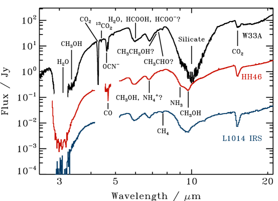
Figure 1: Ice spectra toward the protostars W33A (10⁵ L_⊙), HH46 (12 L_⊙) and L1014 IRS (0.09 L_⊙) from [Gibb et al.(2000), Boogert et al.(2004)] and [Boogert et al.(2008)]. The 3 $\mu$m portions of the spectra have been binned to increase the S/N.

Ices are generally observed in absorption at mid-IR wavelengths and can therefore only be observed in lines of sight with infrared background sources. Protostars are excellent IR sources and ices in protostellar envelopes are the most extensively studied (Fig. 1). Early ice observations were exclusively ground based and thus limited to observe ice bands that coincide with atmospheric windows. IRAS and especially ISO opened up the full infrared spectral region, resulting in the first complete ice inventories toward bright protostars and a few cloud lines of sight. The ISO ice results are described in [Gibb et al.(2004)] and these still constitute the largest high-mass protostellar sample.

Compared to previous space missions, Spitzer’s high sensitivity enabled observations of ices toward low-mass protostars and also toward previously inaccessible background stars. The largest sample was obtained within the $c2d$ program, defined in [Evans et al.(2003)], which included IRS spectra of 50 low-mass protostars. The different ice bands were analyzed in a series of papers by [Boogert et al.(2008)], [Pontoppidan et al.(2008)], [Öberg et al.(2008)] and [Bottinelli et al.(2010)]. Additional Spitzer observations exist on ices toward background sources, looking through molecular clouds at a range of extinctions (reported by [Bergin et al.(2005)], [Knez et al.(2005)], [Pontoppidan(2006)], [Whittet et al.(2009)] and [Boogert et al.(2011)]) and toward protostars in the high-UV environment of IC 1396A by [Reach et al.(2009)]. Because the Spitzer spectrometer had a lower cutoff at $\sim$5 $\mu$m, complete ice inventories can only be obtained by adding complementary ground-based spectroscopy to cover the strong 3 $\mu$m H₂O, the 4.65 $\mu$m CO, the 4.60-4.62 $\mu$m XCN, and the 3.53 $\mu$m CH₃OH features and this was done using VLT and Keck. Results are summarized in Öberg et al. (2011, subm. to ApJ).

The combined Spitzer, ISO, VLT and Keck ice sample spans the full range of observed luminosities from the low-luminosity object L1014 IRS ($<$0.1L_⊙) to the $10^{5}$ L_⊙ massive protostar W33A (Fig. 1). The low-mass young stellar objects (YSOs) are located in Perseus, Taurus, Serpens, Ophiuchus and Corona Australis, as well as a number of nearby isolated dense cores, and thus cover star-forming regions with different histories and physical environments. The sample also represents a wide range of cloud, cloud core and YSO evolutionary stages, from envelope-dominated Class 0 sources to disks.

3 Ice identifications

Figure 1 shows ice spectra toward protostars with the identifications of different bands to H₂O, CO, CO₂, CH₃OH, NH₃, CH₄ and OCN^- ice marked. [van Broekhuizen et al.(2005)] found that the observed XCN band at 4.62 $\mu$m consists of two components. Based on laboratory spectroscopy from [van Broekhuizen et al.(2004)], at least one of the components is due to OCN^-. OCN^- in a separate ice matrix is probably the carrier of the second XCN band component (centered at 2175 cm^-1), but other identifications have also been suggested by e.g. [Fraser et al.(2005)].

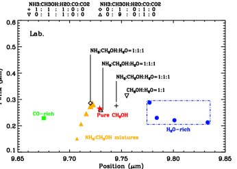
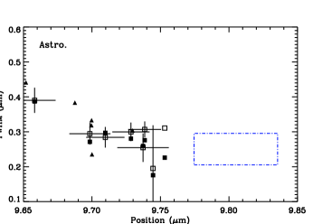
Figure 2: Figure from [Bottinelli et al.(2010)] showing the FWHM and peak position of the CH₃OH feature in laboratory mixtures at 15 K (left panel) and in Spitzer $c2d$ spectra (right panel). In the right panel an increasing symbol size is indicative of increasing CH₃OH content. In both panels, the dash-dot polygons delimitate the parameter space of FWHM and peak positions corresponding to H₂O-rich mixtures.

In general the frequency of a solid state molecular vibration depends on the bonding environment of the vibrating molecule. This results in that the positions and shapes of ice spectroscopic features depend on the ice mixture(s). Fig. 2 from [Bottinelli et al.(2010)] demonstrates how the CH₃OH FWHM and band center depend on the ice mixture in laboratory experiments and how this can be used to constrain that protostellar CH₃OH ices are not present in H₂O-dominated ices.

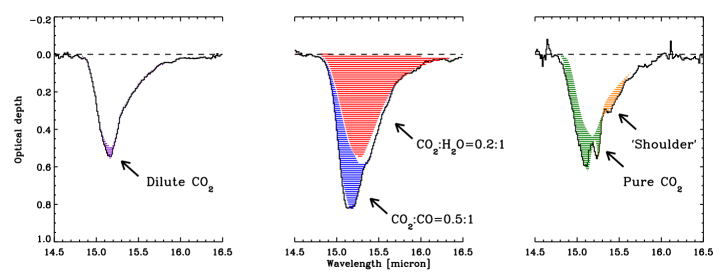
Figure 3: Sketch of the five different components used to fit the CO₂ band on top of IRS 51, SVS 4-5, and RNO 91 spectra from [Pontoppidan et al.(2008)]

Some ice bands, such as CO and CO₂, cannot be fitted by a single laboratory ice mixture, but seem to trace molecules in two or more ice phases, often referred to as polar and apolar. Traditionally the observed spectra have been directly compared to a superposition of laboratory pure and mixed ice spectra to constrain ice components, see e.g. [Merrill et al.(1976)], [Gibb et al.(2004)] and [Zasowski et al.(2009)]. The constraints are often degenerate, however, since ice spectral features vary with ice composition, temperature and radiation processing. To address this, observed ice bands are now commonly decomposed phenomenologically and then the components are compared to laboratory spectra, see [Tielens et al.(1991)], [Pendleton et al.(1999)], [Keane et al.(2001)] and [Boogert et al.(2008)]. Because all observed spectra are decomposed into the same, small number of components, this method provides information on the sample as a whole, i.e. it directly shows which parts of the spectral profile are ubiquitous and which are environment dependent. Figure 3 from [Pontoppidan et al.(2008)] demonstrates how the derived CO₂ ice components can be identified with pure CO₂ ice, CO₂ mixed with CO (CO₂:CO), CO₂ mixed with H₂O ice (CO₂:H₂O) and a shoulder associated with CO₂ mixed with CH₃OH. [Pontoppidan et al.(2003)] showed that the CO ice band can be similarly decomposed into three components corresponding to pure CO ice, CO:CO₂ and CO:H₂O or CO:CH₃OH.

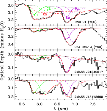
Figure 4: Left panel: Decomposition of the absorption features in the 5-8 $\mu$m spectra of two background stars (bottom panels), compared to two YSOs. The sum of the components is indicated with a thick red line. Figure from [Boogert et al.(2011)]. Right panel: Spectra toward W33A, NGC7538 IRS9 and B1-b, following subtraction of a local spline continuum, plotted together with laboratory spectra of HCOOH, CH₃CHO and CH₃CH₂OH ices. The dashed lines mark the 7.25 and 7.40 $\mu$m features usually assigned to HCOOH and HCOO^-.

Figure 1 also shows tentative identifications to HCOOH and NH${}_{4}^{+}$ in a complex band between 5 and 7 $\mu$m. To constrain the carriers of this band [Boogert et al.(2008)] decomposed it into five different components (C1–C5) after subtraction of the contribution from H₂O ice (Fig. 4). From comparison with laboratory ice spectra, C1 has been identified with HCOOH and H₂CO, C2 with HCOO^- and NH₃, C3 with NH${}_{4}^{+}$ and CH₃OH, C4 with NH${}_{4}^{+}$ and C5 with warm H₂O and anions. The 7.25 $\mu$m has been used to derive HCOOH ice abundances by e.g. [Schutte et al.(1999)], [Gibb et al.(2004)] and [Boogert et al.(2008)]. The right panel of Figure 4 shows that CH₃CH₂OH is an equally plausible carrier, however. The presence of a 7.25 $\mu$m feature is evidence for the formation of complex ices, but derivations of HCOOH abundances from this band is not possible without higher resolution spectra that can distinguish between the two carriers.

4 Ice abundance studies

Following ice identification, ice column densities are determined by dividing the integrated optical depth of the ice feature by the band strength. Ice abundances are expressed with respect to H₂O ice, because H₂O ice is predicted to form early during star formation, is the most abundant ice, and has a high sublimation point. Determining ice abundances is important to predict the chemical evolution in different environments and to constrain the C, O and N budget. In addition to these direct uses, the following sections demonstrate how ice abundance statistics can be used to put constraints on how ices form. Comparison of ice distributions between clouds and protostars constrain which ices require protostellar heating or UV processing to form. Ice abundance variations constrain which ices co-form with H₂O and which ices form in a separate stage. Ice correlations provide further constraints on co-formation, and anti-correlations can be used to demonstrate competitive formation. In these investigations it is key to quantify how significant differences and correlations really are. Finally, ice maps provide direct evidence of how ice formation depends on the position of a source in a cloud or a core.

4.1 Typical abundances

Table 1: Recommended ice abundances toward low- and high-mass protostars and clouds.

Ice feature	Low-mass	High-mass	background
H2O	100	100	100
CO	29	13	31
CO2	29	13	38
CH3OH	3	4	4
NH3	5	5	–
CH4	5	2	–
XCN	0.3	0.6	–
pure CO	21	3	–
CO:H2O	13	10	–
CO:CO2	2	0.3	–
pure CO2	2	2	–
CO2:H2O	20	9	24
CO2:CO	5	5	6
CO2 shoulder	0.8	1	–
OCN-	0.2	0.6	–
2175 cm-1	0.2	0.1	–
C1 (HCOOH + H2CO)a	2.5	2.1	2.8
C2 (HCOO-+NH3)a	1.1	1.3	2.5
C3 (NH${}_{4}^{+}$ + CH3OH)a	4.3	4.3	3.7
C4 (NH${}_{4}^{+}$)a	2.3	4.3	2.1
C5 (warm H2O + anions)a	0.9	1.4	–

^aBecause of multiple band carriers, the reported number is $\tau_{\rm peak}/(N_{\rm H_{2}O}\times 10^{-18})$.

Table 1 lists the representative ice abundances found toward low-mass protostars from the $c2d$ survey, high-mass protostars from [Gibb et al.(2004)]and background stars from [Knez et al.(2005)] and [Boogert et al.(2011)]. The reported median abundances are calculated using the Kaplan-Meier (KM) estimate of the survival function. This is a non-parametric procedure that takes into account the constraints provided by upper limits. When calculating the KM estimate, the detections and upper limits are ordered from low to high and the upper limits are given the values of the nearest lower detections. For example in a sample of four detections of 0.5, 1, 3 and 4 and an upper limit of $<$2, the upper limit is treated as a detection of 1. The KM estimate and how to apply statistical tests on it is reviewed by [Feigelson & Nelson(1985)]. Compared to medians based on only detected ice abundances, the medians calculated from the KM estimate provide more accurate descriptions of ice populations with significant upper limits. The difference is significant, e.g. the CH₃OH and NH₃ medians toward high-mass protostars are 40-70% lower when taking into account the upper limits, resulting in similar abundances toward low- and high-mass YSOs and clouds of 3–5%. The CO and CO₂ abundances vary between the different environments, but are always second in abundance only to H₂O.

4.2 The C, O and N budget

The amount of C, O and N that are typically bound up in ice mantles is important for the life cycle of the elements in the interstellar medium. [Przybilla et al.(2008)] found that the total C, O and N abundances in the solar neighborhood are 2.1, 5.8 and 0.58$\times 10^{-4}$ per hydrogen nuclei, respectively. The fractional C, O and N abundance in ices with respect to these total C, O and N abundances can be calculated from the presented ice abundances with respect to H₂O ice together with a median H₂O abundance with respect to hydrogen of $5\times 10^{-5}n_{\rm H}$ from [Pontoppidan et al.(2004)] and [Boogert & Ehrenfreund(2004)]. The resulting median percentages of C, O and N in ices are 8–16% with respect to the total elemental abundances. When the C and O bound up in grains is subtracted, these values increase to 14–34% (Table 2). For the most ice-rich sources in the sample, the amount of O and C in ice approaches the abundances of volatile O and C, indicative of that ice formation only stops when the gas-phase is completely depleted of these elements.

Table 2: The percentages of C, O and N bound up in protostellar ices.

	Cice / Ctotal	Oice / Ototal	Nice / Ntotal		Cice / Cvol	Oice / Ovol
Low-mass median	15%	16%	10%		27%	34%
Low-mass max	46%	29%	35%		83%	61%
High-mass median	8%	12%	12%		14%	25%
High-mass max	18%	17%	22%		32%	36%

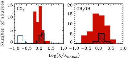
Figure 5: Histograms of CO₂ and CH₃OH toward low-mass protostars (red fill), our background star sample (black line-fill) and Taurus background stars (blue contours).

4.3 Cloud versus protostellar ices

Comparisons between protostars and background stars provide direct limits on which ices form before the protostar turns on and starts to heat and irradiate its surroundings. [Cook et al.(2011)] showed that in Taurus the CO₂ ice fraction in clouds is lower compared to low-mass protostellar envelopes, and proposed that at least some of the CO₂ observed toward protostars forms from energetic processing. Similarly, CH₃OH ice has been proposed to be a product of protostellar UV ice-processing by e.g. [Gibb et al.(2004)]. Figure 5 shows that the CO₂ and CH₃OH ice abundances toward protostars and background stars from [Boogert et al.(2011)] are similar, and that the Taurus CO₂ ice abundances from [Whittet et al.(2007)] are poor templates for ice abundances toward average cloud cores.

[Boogert et al.(2011)] show that there is also no statistically significant difference in the C1-4 components between the protostars and background stars, but the C5 component is absent in cloud sources.The only other feature that is present exclusively toward protostars is pure CO₂ ice, which is proposed to form from thermally induced ice segregation or distillation. The protostar thus seems to have a very limited impact on the observable ice composition. This entails that protostellar ice abundances mainly reflect the ice formation process in the previous cold cloud phase.

4.4 Protostellar ice abundance variations

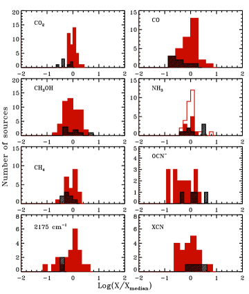
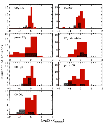
Figure 6: Histograms of ice and ice component abundances toward low-mass (red) and high-mass (black) protostars. The abundances are log-transformed and normalized to the median detected low-mass protostellar ice abundance. Note the difference in spread between species.

Ice abundance variations between different sources depend on how sensitive the ice formation and destruction pathways are to the local environment. Since ice abundances are with respect to H₂O, a small variation of a species indicates co-formation with H₂O, while large ice abundance variations are indicative of different formation and/or destruction dependencies than H₂O ice. Figure 6 shows that the CO₂, CH₄ and NH₃ abundance distributions are narrow, indicative of that these ices form together with H₂O, while the CO, OCN^- and CH₃OH distributions are broad. The ice abundances around high-mass protostars are generally lower compared to low-mass protostars, indicating that heat and UV mainly destroy simple ices. The large CH₃OH, CO and OCN^- abundance variations must then originate from a separate prestellar ice formation stage compared to the stage associated with H₂O formation. This is consistent with observations that most prestellar and protostellar CO₂ is present in a H₂O rich ice, while CH₃OH and CO ices are not. Figure 6 shows the distributions of the individual CO and CO₂ components. The pure CO and CO₂ ice components have the broadest distributions, consistent with their expected dependence on the protostellar envelope temperature for ice evaporation and segregation. All other CO and CO₂ component distributions, except for CO₂:H₂O, are broad as well, indicative of a different history compared to the H₂O-rich ice phase.

4.5 Ice maps

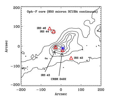
Figure 7: Left panel: The locations of the sources used to construct the ice map plotted on the SCUBA 850 $\mu$m map from [Pontoppidan(2006)] with respect to the central core (star). Right panel: Ice abundances at different distances from the Oph-F core with respect to H₂O ice. The 2175 cm^-1 abundances are scaled by 40 and the CO₂:CO abundances by 5 for clarity.

The spatial extent of ices can be mapped in clouds and cloud cores if enough background sources are available. Mapping of ice abundances in dense clouds by [Bergin et al.(2005)] has revealed a similar formation threshold of H₂O and CO₂ at A_V=4 mag. CO is only observed at higher extinctions. The H₂O-rich ice thus forms first.

[Pontoppidan et al.(2008)] shows that toward the Oph-F core, where protostars are used as background sources to probe the cloud core ices, CO ice abundances increase dramatically toward the core (Fig. 7). [Pontoppidan(2006)] interpreted this as catastrophic freeze-out of CO in the pre-stellar stage once a certain density and temperature is reached. Figure 7 shows that the order of magnitude increase in CO ice with respect to H₂O toward the core is accompanied by an increase in CO₂:CO. In contrast, the CO₂:H₂O ice component is almost constant. CO:H₂O and XCN band are the only other species that increase monotonically toward the densest part of Oph-F core. These bands thus appear directly related to CO freeze-out, indicating that their broad abundance distributions in Fig. 6 are due to their dependence on the prestellar CO freeze-out level. No trend with distance to the core center is seen or expected for ices that form with H₂O (e.g. CH₄ and NH₃), or of species dependent on protostellar heating (e.g. pure CO₂ ice) or of components with potentially multiple carriers, such as the C1-5 bands. CH₃OH is only detected toward one of the sources and no trend can be extracted.

4.6 Ice abundance correlations

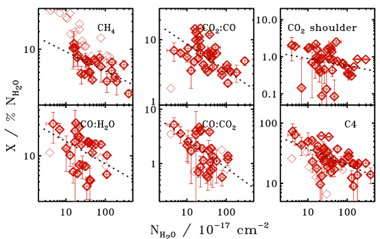
Figure 8: Statistically significant correlations between ice abundances w. r. t. H₂O (N_X / % N${}_{\rm H_{2}O}$) and the H₂O ice column density for low-mass protostars, with upper limits plotted with thin symbols. The significance of the correlations was measured using Spearman’s rank correlation test, which makes no assumptions about the type of correlation, while the dotted line shows the best log-log fit to the data to guide the eye.

Ice maps are extremely useful, but only possible in a few lines of sight with fortuitous placement of background sources. Ice correlation tests is another tool used to constrain the ice formation history, used by e.g. [Boogert et al.(2008)] to investigate which ice components depend on ice heating to form. Figure 8 shows an example of such a correlation study using the $c2d$ low-mass protostellar sample. Among the investigated ices, the abundance w.r.t H₂O of CH₄, CO₂:CO, the CO₂ shoulder, CO:H₂O, CO:CO₂ and C4 are anti-correlated with the H₂O column density at 97–99% confidence with the rank correlation test introduced by [Spearman(1904)]. The CO-related anti-correlations are consistent with the §4.5 results that H₂O-rich and a CO-rich ice phases form separately in clouds and cloud cores. The anti-correlations are expected if there is competition between the formation of these two phases; i.e. the more oxygen that is bound up in H₂O ice, the less may be available to form CO and thus ices that depend on CO freeze-out. Still in each individual core CO ice abundance and H₂O ice column are expected to correlate because of increasing CO freeze-out toward the densest part of the cloud core. This accounts for some of the scatter in the plots. The CH₄–H₂O trend is strongest for low H₂O column densities and may be due to more efficient CH₄ formation during the earliest H₂O formation stage when then C/CO ratio is high.

5 An ice evolution scenario

Building on the presented results above as well as additional experiments, models and observations, this section discusses what the current constraints on the ice evolution from clouds to protostars.

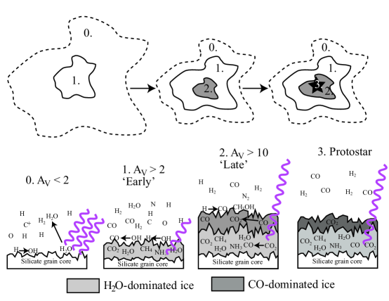
Figure 9: The key ice reactions during cloud and star formation, where 0. corresponds to cloud edges where UV photons can penetrate, 1. the early stages of dense cloud formation, 2. the later formation of cloud cores and 3. the protostellar envelope. Ice formation begins in 1. with hydrogenation of atoms resulting in a H₂O dominated ice with a high CO₂ concentration (CO₂:H₂O). At later times CO freezes out catastrophically, resulting in a second layer where CO₂ formation continues (CO₂:CO) and CH₃OH formation begins. Small amounts of ice surface chemistry products are maintained in gas-phase due to non-thermal desorption. In the protostellar stage desorption of CO starts at 20 K and H₂O:CO₂ segregation at 30 K.

5.1 Ice formation in clouds and cloud cores

From ice maps of cloud edges, the first ices to form are H₂O dominated with large concentrations of CO₂ (Fig. 9). CH₄ formation is the most efficient at the earliest stages of H₂O ice formation, when the C/CO ratio in the gas phase is still high (§4.6). The narrow abundance distribution of NH₃ is evidence for that it too forms with H₂O. This ice formation stage depend on hydrogenation of atoms, O+H, C+H and N+H; CO₂ can form efficiently from CO+OH at low temperatures, based on experiments by [Oba et al.(2010)], [Ioppolo et al.(2011)] and [Noble et al.(2011)]. Most CO that is frozen out in this phase must be converted into CO₂ since CO₂:H₂O is more abundant than CO:H₂O. From experiments by [Hiraoka et al.(1998)], H preferentially reacts with atoms compared to CO, explaining why no CH₃OH forms in this ice formation phase.

At some point the CO/O ratio becomes large enough that most frozen-out CO is no longer converted into CO₂ and H₂O is no longer the most efficiently formed ice. We mark this as the breaking point between early H₂O dominated and late CO-driven pre-stellar ice formation. The ices that form in this later stage are not expected to co-vary with H₂O, but rather depend on the CO-freeze-out efficiency. The latter is both temperature and density dependent and may vary greatly dependent on cloud structure, cloud collapse time scales and local radiation environment. This explains why many identified ice and ice components that are definitely present during the pre-stellar stage have abundances that vary by orders of magnitude with respect to H₂O. In addition, the anti-correlation between H₂O ice and the abundance of several CO-ice components suggest that the time available for this CO-based chemistry decreases when a longer time is spent in the H₂O-ice formation stage, where O is converted into H₂O and CO₂:H₂O ice .

CO₂:CO, CO:H₂O and the XCN band all correlate with CO freeze-out in the Oph-F ice map. CO₂ may still form from OH+CO at this stage, but a high CO/O ratio results in sparse H₂O formation compared to CO and thus in a CO-rich CO₂ ice. This is also the outcome from recent modeling by [Garrod & Pauly(2011)]. OCN^- may form from CO+NH, followed by proton transfer, and the XCN-CO freeze-out correlation supports that OCN^- is responsible for the entire XCN band. [Cuppen et al.(2009)] have used recent experiments to show that CH₃OH and H₂CO can form from hydrogenation of CO under ISM conditions and CH₃OH abundance should also depend on CO freeze-out. In addition to atomic processing, the ices are continuously exposed to cosmic rays and cosmic-ray induced UV photons – [Shen et al.(2004)] have estimated the relative doses. This may both affect the simple ice abundances and result in some cold formation of more complex molecules.

5.2 Thermal and UV processing of ices around protostars

Though much of the observed ice evolution can be explained by processes during the prestellar stage, some ice features are formed or destroyed by the protostar. Based on the observations of pure CO₂ by [Pontoppidan et al.(2008)] and experiments by e.g. [Öberg et al.(2009b)], evaporation of CO from CO₂:CO ice and segregation of H₂O:CO₂ ices are efficient above 20–30 K in protostellar envelopes. Pure CO₂ is also observed by [Kim. et al.(2011)] around extremely low-luminosity protostars, however, and may there be a remnant of past outbursts that heated up the envelope beyond its low-accretion temperature, since ice segregation is an irreversible process. [Evans et al.(2009)] and [Dunham et al.(2010)] have invoked episodic accretion to explain the luminosity problem of low-mass YSOs, i.e. the observation that most YSOs are significantly less luminous than predicted by protostellar evolutionary models with steady accretion.

The observed lower CO and CH₄ ice abundances toward high-mass protostars compared to low-mass YSOs can also be explained by protostellar ice heating since these are very volatile ices. From experiments by e.g. [Sandford & Allamandola(1990)], [Collings et al.(2004)] and [Fayolle et al.(2011)], some CO and CH₄ can be trapped in H₂O ices, however, which is important for predicting ice abundances in moderately heated regions, such as the comet forming zones in protoplanetary disks.

From experiments by e.g. [Öberg et al.(2009a)], moderate ice heating to 20–50 K also enables the movement of radicals within the ice. Radicals are produced in ices by photodissociation of the condensed molecules. Models by [Garrod et al.(2008)] predict that especially CH₃OH photodissociation followed by radical diffusion result in complex ice formation and protostellar envelopes are thus expected to be efficient factories of complex organics. UV radiation of CO:CH₃OH ice mixtures produce a more HCO-rich complex chemistry, which may dominate at lower temperatures when CO is still frozen out. The ice feature at 7.25 $\mu$m identified with to HCOOH or CH₃CH₂OH provides direct evidence for this complex ice chemistry. Most complex ice features cannot be directly observed, however, because of band confusion. Instead most constraints on this ice evolutionary phase comes from millimeter observations of desorbed ice chemistry products.

Complex organic molecules such as CH₃CH₂OH and HCOOCH₃ are observed in the inner regions around high-mass protostars, in so called hot cores, at abundances that cannot be reproduced by gas phase chemistry. Furthermore, [Bisschop et al.(2007)] found that they correlate with the ice chemistry product CH₃OH. These observational pieces of evidence, together with the existence of a plausible ice production pathway of complex molecules, strongly support a scenario in which complex ices are produced in the outer envelope and then desorb into the gas-phase as icy grains flow in towards the protostar.

IRAS 16293-2422, observed by e.g. [van Dishoeck et al.(1995)] and [Cazaux et al.(2003)] is a low-mass equivalent to the high-mass hot cores, and there are at least five other low-mass protostars where complex molecules such as HCOOCH₃ and CH₃OCH₃ are detected by [Bottinelli et al.(2004)], [Jørgensen et al.(2005)] and [van der Marel et al.(2011)]. [Arce et al.(2008)] also detected complex molecules in a low-mass outflow and [Öberg et al.(2010)] recently detected HCOOCH₃ in a cold and quiescent part of a low-mass star forming region that probably has been illuminated by UV through a protostellar outflow cavity. Combining these observational results, Öberg et al. (2011b, subm. to ApJ) find that HCOOCH₃ generally dominates the complex chemistry toward outflows and low-mass protostellar envelopes, consistent with experiments on CO:CH₃OH ice photochemistry below 25 K. In contrast, observations of high-mass and resolved low-mass hot cores contain more CH₃OCH₃ or C₂H₅OH than HCOOCH₃. This is evidence for a sequential formation of complex molecules, starting with HCO-rich molecules as long as CO ice is abundant, followed by CH_3/2-rich molecules at higher ice temperatures. Gas phase observations can thus provide information on the ice chemistry, but interpretations of these more indirect constraints rely on a combination of experimental and model results.

6 Conclusions

Thanks to a combination of ground-based and space telescope ice observations and years of laboratory ice spectroscopy and ice chemistry experiments we have good constraints on the typical ice abundances and ice compositions in a range of interstellar and circumstellar environments. A key result coming out of these observations is that most ices up to CH₃OH in complexity have already formed by the time the protostar turns on. Ice abundance variations must therefore be mainly due to variations in the prestellar ice formation processes. Variations in CO freeze-out and the subsequent CO-based chemistry is a likely main contributor to the observed differences in ice abundances in different lines of sight, but other processes may be important as well. Thermal and UV processing of ices by the protostar is important for the continued evolution of the ice, leading up to the formation of hot core molecules and the complex organics found in comets. To further constrain the ice evolution from cloud cores to comets will require a combination of high-resolution IR studies to detect complex molecules directly in the ice, millimeter observations toward protostars and disks to image desorbed ice chemistry products, and more detailed experiments and models of both the early ice formation stages and of the reactions that convert simple ices into more complex ones.

Amanda CookAt least once in your talk you referred to a pure CO₂ component in the ice. Since it seems like CO₂ and H₂O forms in tandem in molecular clouds, how would you explain the presence of pure CO₂ ice?

ÖbergPure CO₂ ice can form from evaporation of CO at 20 K from the CO₂:CO ice layer that is a result of late CO₂ formation in cloud cores, or from segregation of the H₂O:CO₂ ice layer starting at 30 K. Pure CO₂ is therefore only expected in environments where ices have been heated to at least 20–30 K.

Name SakaiWhat is the origin of the difference of molecular abundances in the ice between low-mass and high-mass sources? Are the ice abundances in high-mass cases measured in pre-stellar cores?

ÖbergThe high-mass sources are all protostars. Low CO and CH₄ ice abundances toward high-mass YSOs are probably due to that the protostars have heated most of the envelopes, resulting in evaporation of volatile ices. The difference in CO₂ ice abundances may be due to either CO₂ evaporation in the high-mass protostellar envelope, or due to less CO₂ formation in the high-mass pre-stellar phase because of different collapse time scales, and density and temperature structures in low- and high-mass prestellar cores

Jacob LaasThe recent studies by Gerakines et al. have found that NH₃ and other N-bearing species can have large effects on certain line profiles in ices. Could this have any effect on the spectral signatures near 7$\mu$m that you say are strong indicators of complex organic molecules?

ÖbergNH₃ acts as a base in ices, transforming e.g. HCOOH into HCOO^-. If the two bands at 7.2–7.5 $\mu$m are due (partially) to HCOOH and HCOO^-, NH₃ may regulate the relative intensities of the two bands. If the bands are instead due to CH₃CH₂OH and CH₃CHO, NH₃ should not have a large effect on the band characteristics.

References

- [Arce et al.(2008)] Arce, H. G., Santiago-García, J., Jørgensen, et al. 2008, ApJl, 681, L21
- [Bergin et al.(2005)] Bergin, E. A., Melnick, G. J., Gerakines, P. A., et al. 2005, ApJl, 627, L33
- [Bisschop et al.(2007)] Bisschop, S. E., Jørgensen, J. K., van Dishoeck, E. F. et al. 2007b, A&A, 465, 913
- [Boogert & Ehrenfreund(2004)] Boogert, A. C. A. & Ehrenfreund, P. 2004, in ASP Conf. Ser. 309: Astrophysics of Dust, 547–572
- [Boogert et al.(2011)] Boogert, A. C. A., Huard, T. L., Cook, A. M., et al. 2011, ApJ, 729, 92
- [Boogert et al.(2008)] Boogert, A. C. A., Pontoppidan, K. M., Knez, C., et al. 2008, ApJ, 678, 985
- [Boogert et al.(2004)] Boogert, A. C. A., Pontoppidan, K. M., Lahuis, F., et al. 2004, ApJs, 154, 359
- [Bottinelli et al.(2010)] Bottinelli, S., Adwin Boogert, A. C., Bouwman, J., et al. 2010, ApJ, 718, 1100
- [Bottinelli et al.(2004)] Bottinelli, S., Ceccarelli, C., Neri, R., et al. 2004, ApJl, 617, L69
- [Cazaux et al.(2003)] Cazaux, S., Tielens, A. G. G. M., Ceccarelli, C., et al. 2003, ApJl, 593, L51
- [Charnley(2004)] Charnley, S. B. 2004, Advances in Space Res., 33, 23
- [Charnley et al.(1992)] Charnley, S. B., Tielens, A. G. G. M., & Millar, T. J. 1992, ApJl, 399, L71
- [Collings et al.(2004)] Collings, M. P., Anderson, M. A., Chen, R., et al. 2004, MNRAS, 354, 1133
- [Cook et al.(2011)] Cook, A. M., Whittet, D. C. B., Shenoy, S. S., et al. 2011, ApJ, 730, 124
- [Cuppen et al.(2009)] Cuppen, H. M., van Dishoeck, E. F., Herbst, E., & Tielens, A. G. G. M. 2009, A&A, 508, 275
- [D’Hendecourt & Jourdain de Muizon(1989)] D’Hendecourt, L. B. & Jourdain de Muizon, M. 1989, A&A, 223, L5
- [Dunham et al.(2010)] Dunham, M. M., Evans, N. J., Bourke, T. L., et al. 2010, ApJ, 721, 995
- [Evans et al.(2009)] Evans, N. J., Dunham, M. M., Jørgensen, J. K., et al. 2009, ApJs, 181, 321
- [Evans et al.(2003)] Evans, II, N. J., Allen, L. E., Blake, G. A., et al. 2003, PASP, 115, 965
- [Fayolle et al.(2011)] Fayolle, E. C., Öberg, K. I., Cuppen, H. M., Visser, R., & Linnartz, H. 2011, A&A, 529, A74+
- [Feigelson & Nelson(1985)] Feigelson, E. D. & Nelson, P. I. 1985, ApJ, 293, 192
- [Fraser et al.(2005)] Fraser, H. J., Bisschop, S. E., Pontoppidan, K. M., et al. 2005, MNRAS, 356, 1283
- [Garrod & Pauly(2011)] Garrod, R. T. & Pauly, T. 2011, ArXiv e-prints
- [Garrod et al.(2008)] Garrod, R. T., Weaver, S. L. W., & Herbst, E. 2008, ApJ, 682, 283
- [Gibb et al.(2004)] Gibb, E. L., Whittet, D. C. B., Boogert, A. C. A., & Tielens, A. G. G. M. 2004, ApJs, 151, 35
- [Gibb et al.(2000)] Gibb, E. L., Whittet, D. C. B., Schutte, W. A., et al. 2000, ApJ, 536, 347
- [Gillett & Forrest(1973)] Gillett, F. C. & Forrest, W. J. 1973, ApJ, 179, 483
- [Hiraoka et al.(1998)] Hiraoka, K., Miyagoshi, T., Takayama, T., Yamamoto, K., & Kihara, Y. 1998, ApJ, 498, 710
- [Ioppolo et al.(2011)] Ioppolo, S., van Boheemen, Y., Cuppen, H. M., et al. H. 2011, MNRAS, 238
- [Jørgensen et al.(2005)] Jørgensen, J. K., Bourke, T. L., Myers, P. C., et al. 2005, ApJ, 632, 973
- [Keane et al.(2001)] Keane, J. V., Boonman, A. M. S., Tielens, A. G. G. M., et al. 2001, A&A, 376, L5
- [Kim. et al.(2011)] Kim., H. J., Evans, II, N. J., Dunham, M. M., & Lee, J. E. 2011, in IAU Symposium, 280, 216
- [Knez et al.(2005)] Knez, C., Boogert, A. C. A., Pontoppidan, K. M., et al. 2005, ApJl, 635, L145
- [Merrill et al.(1976)] Merrill, K. M., Russell, R. W., & Soifer, B. T. 1976, ApJ, 207, 763
- [Oba et al.(2010)] Oba, Y., Watanabe, N., Kouchi, A., Hama, T., & Pirronello, V. 2010, ApJl, 712, L174
- [Öberg et al.(2008)] Öberg, K. I., Boogert, A. C. A., Pontoppidan, K. M., et al. 2008, ApJ, 678, 1032
- [Öberg et al.(2010)] Öberg, K. I., Bottinelli, S., Jørgensen, J. K., & van Dishoeck, E. F. 2010, ApJ, 716, 825
- [Öberg et al.(2009b)] Öberg, K. I., Fayolle, E. C., Cuppen, H. M., et al., H. 2009a, A&A, 505, 183
- [Öberg et al.(2009a)] Öberg, K. I., Garrod, R. T., van Dishoeck, E. F., & Linnartz, H. 2009, A&A, 504, 891
- [Noble et al.(2011)] Noble, J. A., Dulieu, F., Congiu, E., & Fraser, H. J. 2011, ApJ, 735, 121
- [Pendleton et al.(1999)] Pendleton, Y. J., Tielens, A. G. G. M., Tokunaga, A. T., et al. 1999, ApJ, 513, 294
- [Pontoppidan(2006)] Pontoppidan, K. M. 2006, A&A, 453, L47
- [Pontoppidan et al.(2008)] Pontoppidan, K. M., Boogert, A. C. A., Fraser, H. J., et al. 2008, ApJ, 678, 1005
- [Pontoppidan et al.(2003)] Pontoppidan, K. M., Dartois, E., van Dishoeck, E. F., et al. 2003a, A&A, 404, L17
- [Pontoppidan et al.(2003)] Pontoppidan, K. M., Fraser, H. J., Dartois, E., et al. 2003b, A&A, 408, 981
- [Pontoppidan et al.(2004)] Pontoppidan, K. M., van Dishoeck, E. F., & Dartois, E. 2004, A&A, 426, 925
- [Przybilla et al.(2008)] Przybilla, N., Nieva, M., & Butler, K. 2008, ApJl, 688, L103
- [Reach et al.(2009)] Reach, W. T., Faied, D., Rho, J., et al. 2009, ApJ, 690, 683
- [Sandford & Allamandola(1990)] Sandford, S. A. & Allamandola, L. J. 1990, ApJ, 355, 357
- [Schutte et al.(1999)] Schutte, W. A., Boogert, A. C. A., Tielens, A. G. G. M., et al. 1999, A&A, 343, 966
- [Shen et al.(2004)] Shen, C. J., Greenberg, J. M., Schutte, W. A., & van Dishoeck, E. F. 2004, A&A, 415, 203
- [Spearman(1904)] Spearman, C. 1904, The American Journal of Psychology, 15, pp. 72
- [Tielens & Hagen(1982)] Tielens, A. G. G. M. & Hagen, W. 1982, A&A, 114, 245
- [Tielens et al.(1991)] Tielens, A. G. G. M., Tokunaga, A. T., Geballe, T. R., & Baas, F. 1991, ApJ, 381, 181
- [van der Marel et al.(2011)] van der Marel, N., Öberg, K. I., Kristensen, L., et al., 2011, IAU Symposium 280, 365
- [van Broekhuizen et al.(2004)] van Broekhuizen, F. A., Keane, J. V., & Schutte, W. A. 2004, A&A, 415, 425
- [van Broekhuizen et al.(2005)] van Broekhuizen, F. A., Pontoppidan, K. M., Fraser, H. J., et al. 2005, A&A, 441, 249
- [van Dishoeck et al.(1995)] van Dishoeck, E. F., Blake, G. A., Jansen, D. J., & Groesbeck, T. D. 1995, ApJ, 447, 760
- [Whittet et al.(2009)] Whittet, D. C. B., Cook, A. M., Chiar, J. E., et al. 2009, ApJ, 695, 94
- [Whittet et al.(2007)] Whittet, D. C. B., Shenoy, S. S., Bergin, E. A., et al. 2007, ApJ, 655, 332
- [Zasowski et al.(2009)] Zasowski, G., Kemper, F., Watson, D. M., et al. 2009, ApJ, 694, 459