Piecewise linear car-following modeling

Abstract

We present a traffic model that extends the linear car-following model as well as the min-plus traffic model (a model based on the min-plus algebra). A discrete-time car-dynamics describing the traffic on a 1-lane road without passing is interpreted as a dynamic programming equation of a stochastic optimal control problem of a Markov chain. This variational formulation permits to characterize the stability of the car-dynamics and to calculte the stationary regimes when they exist. The model is based on a piecewise linear approximation of the fundamental traffic diagram.

1 Introduction

Car-following models are microscopic traffic models that describe the car-dynamics with stimulus-response equations expressing the drivers’ behavior. Each driver responds, by choosing its speed or acceleration, to a given stimulus that can be composed of many factors such as inter-vehicular distances, relative velocities, instantaneous velocities, etc. We present in this article a car-following model that extends the linear car-following model [5, 21, 14, 13], as well as the min-plus traffic model [27].

The vehicular traffic on a 1-lane road without passing is described by discrete-time dynamics, which are interpreted as dynamic programming equations associated to stochastic optimal control problems of Markov chains. The discrete-time variational formulation we make here is similar to the time-continuous one used by Daganzo and Geroliminis [7] to show the existence of a concave macroscopic fundamental diagram.

We are concerned in this article by microscopic traffic modeling with a Lagrangian description of the traffic dynamics, where the function $x(n,t)$, giving the position of car $n$ at time $t$ (or the cumulated distance traveled by a car $n$ up to time $t$), is used. In the macroscopic kinematic traffic modeling, Eulerian descriptions of the traffic dynamics are usually used, with the function $n(t,x)$ giving the cumulated number of cars passing through position $x$ up to time $t$ (which coincides with the Moscowitz function [6] in the case of traffic without passing). The combination of a conservation law with an equilibrium law gives the well known first order traffic model of Lighthill, Whitham and Richards [26, 29].

In this introduction, we first notice that the same approach used in macroscopic traffic modeling, combining a conservation law with an equilibrium law, can be used to derive microscopic traffic models. By this, we introduce car-following models and give a review on basic and most important existing ones. In particular, we recall the linear and the min-plus car-following models, which are particular cases of the model we present here. Finally, we recall a theoretical result on non-expansive and connected dynamic systems which we need in our developments, and give the outline of this article.

The first order partial derivative of the function $x(n,t)$ in time, denoted $\dot{x}(n,t)$ expresses the velocity $v(n,t)$ of car $n$ at time $t$. The first order differentiation of $x(n,t)$ in the car numbers $\Delta x(n,t)$ expresses the inverse of the inter-vehicular distance $y(n,t)=x(n-1,t)-x(n,t)$ between cars $n$ and $n-1$ at time $t$. The equality of the second derivatives $\Delta\dot{x}(n,t)$ and $\dot{\Delta}x(n,t)$ gives then the following conservation law of distance.

$$\dot{y}(n,t)=-\Delta v(n,t).$$ (1)

If we assume that a fundamental diagram $V_{e}$, giving the velocity $v$ as a function of the inter-vehicular distance $y$ ($v=V_{e}(y)$) at the stationary traffic, exists, and that the diagram $V_{e}$ holds also on the transient traffic, then we have

$$\dot{y}(n,t)=\dot{v}(n,t)/V_{e}^{\prime}(y),$$ (2)

where $V_{e}^{\prime}(y)$ denotes the derivative of $V_{e}$ with respect to $y$.

By combining (1) and (2) we obtain the model:

$$\dot{v}(n,t)=-V_{e}^{\prime}(y(n,t))\Delta v(n,t).$$ (3)

(3) is a car-following model that gives the acceleration of car $n$ at time $t$ as a response to a stimulus composed of the relative speed $\Delta v(n,t)$ and the term $V_{e}^{\prime}(y(n,t))$. For example, if $V_{e}(y)=v_{0}\exp{-a/y}$, where $v_{0}$ denotes the free (or desired) velocity, and $a$ is a parameter, then $V^{\prime}(y)=aV(y)/y^{2}$ and (3) gives a particular case of the Gazis, Herman, and Rothery model [13].

The simplest car-following model is the linear one, where the car dynamics are written

$$\dot{x}_{n}(t+T)=a(x_{n-1}(t)-x_{n}(t))+b,$$ (4)

where $T$ is the reaction time, $a$ is a sensitivity parameter, and $b$ is a constant. That model can be derived from (3) with a linear fundamental diagram $V_{e}$. The stability of the linear car-following model (4) and the existence of a stationary regime have been treated in [21].

Almost all car following models are based on the assumption of the existence of a behavioral law $V_{e}$. The latter has been taken linear in [17, 21], logarithmic in [16], exponential in [28], and with more complicated forms in other works. Bando et al. [3] used the sigmiudal function

$$V_{e}(y)=tanh(y-h)+tanh(h),$$ (5)

where $tanh$ denotes the hyperbolic tangent function, and $h$ is a constant.

Kerner and Konhäuser[24], Hermann and Kerner [22], and then Lenz et al.[25], and Hoogendoorn et al. [23] have used the function

$$V_{e}(y)=v_{0}\left\{\left[1+exp\left(\frac{1,000}{\gamma\cdot y}-\frac{10}{2.1}\right)\right]^{-1}-5.34\cdot 10^{-9}\right\},$$ (6)

where free velocity $v_{0}$ and $\gamma$ are parameters estimated from data. In [25], $\gamma$ is taken equal to $7.5$. See also [19, 20, 30].

The min-plus traffic model [27] is a microscopic discrete-time car-following model based on the min-plus algebra [2]. It consists in the following dynamics.

$$x_{n}(t+1)=\min\{x_{n}(t)+v_{0},x_{n-1}(t)-\sigma\},$$ (7)

where $v_{0}$ is the free velocity and $\sigma$ is a safety distance.

The idea of the model (7) is that the car dynamics is linear in the min-plus algebra [2], where the addition is the operation “$\min$” and the product is the standard addition “$+$”. In [27], the dynamic system (7) is written in min-plus notations $x(t)=A\otimes x(t-1)$, where $A$ is a min-plus matrix and $\otimes$ is the min-plus product of matrices. It is then proved that the average growth rate vector per time unit of the system, defined by $\chi=\lim_{t\to\infty}x(t)/t$ satisfies $\chi=(\bar{v},\bar{v},\cdots,\bar{v})$, where $\bar{v}$ is the unique min-plus eigenvalue of the matrix $A$, interpreted as the stationary car-speed. The fundamental diagram is then obtained

$$\bar{v}=\min(v_{0},\bar{y}-\sigma)$$ (8)

$$\bar{q}=\min(v_{0}\bar{\rho},1-\sigma\bar{\rho}),$$ (9)

where $\bar{y},\bar{q}$ and $\bar{\rho}$ denote respectively the equilibrium inter-vehicular distance, car-flow and car-density.

In (7), for $t\geq 0$, if $x_{n-1}(t)-x_{n}(t)>v_{0}+\sigma$, then the dynamics is $x_{n}(t+1)-x_{n}(t)=v_{0}$. If $x_{n-1}(t)-x_{n}(t)\leq v_{0}+\sigma$ then the dynamics is $x_{n}(t+1)-x_{n}(t)=x_{n-1}(t)-x_{n}(t)-\sigma$. Therefore, (7) is linear in both phases of free and congested traffic. The min-plus model (7) permits to distinguish two phases in which the traffic dynamics is linear, but with a sensitivity parameter ($a$ in (4)) equals to $1$ for each phase. The linear model (4) is not constrained in the sensitivity parameter value, but it permits the modeling of only one traffic phase. The model we present here extends (4) and (7) in a way that an arbitrary number of traffic phases can be modeled, with flexibility in the sensitivity parameter value on each phase.

For our model, we apply a similar but more general approach than the min-plus one used to analyze the dynamic system (7). Indeed, the dynamics (7) is additive homogeneous of degree one  and is monotone . It is then non expansive  [4]. The stability of the dynamic system (7) is thus guaranteed from its non expansiveness. Moreover, (7) is connected (or communicating)  [11, 12]. An important result from [18, 11] (Theorem 1 below) permits the analysis of non expansive and connected dynamic systems.

Theorem 1.

[18, 11] If a dynamic system $x(t)=f(x(t-1))$ is non expansive and connected, then the additive eigenvalue problem $\bar{v}+x=f(x)$ admits a solution $(\bar{v},x)$, where $x$ is defined up to an additive constant, not necessarily in a unique way, and $\bar{v}\in\mathbb{R}^{n}$ is unique. Moreover, the dynamic system admits an average growth rate vector $\chi$, which is unique (independent of the initial condition) and given by $\chi(f)={}^{t}(\bar{v},\bar{v},\cdots,\bar{v})$.

The model treated in this article can be seen as an extension of the min-plus model (7). In Section 2, we present the model. It is called piecewise linear car-following model because it is based on a piecewise linear fundamental diagram $V_{e}$. The model describes the traffic of cars on a ring road of one lane without passing. The stability conditions of the dynamic system describing the traffic are determined. Under those conditions, the car-dynamics are interpreted as a dynamic programming equation (DPE) associated to a stochastic optimal control problem of a Markov chain. The DPE is solved analytically. We show that the individual behavior law $V_{e}$ supposed in the model is realized on the collective stationary regime. Finally, the effect of the stability condition on the shape of the fundamental diagram is shown.

In section 3, we give equivalent results of those given in section 2 for the traffic on an “open” road (a highway stretch for example), and conclude with an example, where we simulate the transient traffic, basing on a piecewise linear approximation of the diagram (6).

In B, we give more details on the duality in traffic modeling, of using the functions $n(t,x),x(n,t)$ and $t(n,x)$, where $t(n,x)$ denotes the time of passage of the $n$th car by position $x$.

2 Piecewise linear car following model

The behavioral law $V_{e}$ is an increasing curve bounded by the free speed $v_{0}$. Moreover, $V_{e}(y)=0$ for $y\in[0,y_{j}]$ where $y_{j}$ denotes the jam inter-vehicular distance. We propose here to approximate the curve $V_{e}$ with a piecewise-linear curve

$$V_{e}(y)=\min_{u\in\mathcal{U}}\max_{w\in\mathcal{W}}\{\alpha_{uw}y+\beta_{uw}\},$$ (10)

where $\mathcal{U}$ and $\mathcal{W}$ are two finite sets of indices. Since $V_{e}$ is increasing, we have $\alpha_{uw}\geq 0,\forall(u,w)\in\mathcal{U}\times\mathcal{W}$.

We are interested here on the discrete-time first-order dynamics

$$x_{n}(t+1)=x_{n}(t)+\min_{u\in\mathcal{U}}\{\alpha_{u}(x_{n-1}(t)-x_{n}(t))+\beta_{u}\},$$ (11)

and

$$x_{n}(t+1)=x_{n}(t)+\min_{u\in\mathcal{U}}\max_{w\in\mathcal{W}}\{\alpha_{uw}(x_{n-1}(t)-x_{n}(t))+\beta_{uw}\}.$$ (12)

It is clear that (12) extends (11). The model (12) is also an extension of both linear model (4) and min-plus model (7).

In this article, we characterize the stability of the dynamics (12), calculate the stationary regimes, show that the fundamental diagrams are effectively realized at the stationary regime, and analyze the transient traffic. We will distinguish two cases: Traffic on a ring road and traffic on an “open” road.

2.1 Traffic on a ring road

We follow here the modeling of [27]. Let us consider $\nu$ cars moving a one-lane ring road in one direction without passing. We assume that the cars have the same length that we take here as the unity of distance. The road is assumed to be of size $\mu$; that is, it can contain at most $\mu$ cars. The car density on the road is thus $\rho=\nu/\mu$.

Stochastic optimal control model

We consider here the car dynamics (11). That is to say that each car $n$ maximizes its velocity at time $t$ under the constraints

$$x_{n}(t+1)\leq x_{n}(t)+\alpha_{u}(x_{n-1}(t)-x_{n}(t))+\beta_{u},\quad\forall u\in\mathcal{U}.$$ (13)

Each constraint of (13) bounds the velocity $x_{n}(t+1)-x_{n}(t)$ by a sum of a fixed term $\beta_{u}$ and a term depending linearly on the inter-vehicular distance.

Let us first notice that (11), on the ring road, is written

$$x_{n}(t+1)=x_{n}(t)+\min_{u\in\mathcal{U}}\{\alpha_{u}(x_{n-1}(t)-x_{n}(t))+\beta_{u}\},\quad\text{ for }n\geq 2,$$

$$x_{1}(t+1)=x_{1}(t)+\min_{u\in\mathcal{U}}\{\alpha_{u}(x_{n}(t)+\mu-x_{1}(t))+\beta_{u}\},$$

which can also be written

$$x_{n}(t+1)=\min_{u\in\mathcal{U}}\{(1-\alpha_{u})x_{n}(t)+\alpha_{u}x_{n-1}(t)+\beta_{u}\},\quad\text{ for }n\geq 2,$$

$$x_{1}(t+1)=\min_{u\in\mathcal{U}}\{(1-\alpha_{u})x_{1}(t)+\alpha_{u}x_{n}(t)+\alpha_{u}\nu/\rho+\beta_{u}\}.$$

Let us denote by $M^{u},u\in\mathcal{U}$ the family of matrices defined by

$$M^{u}=\begin{bmatrix}1-\alpha_{u}&0&\cdots&\alpha_{u}\\ \alpha_{u}&1-\alpha_{u}&&0\\ \vdots&\ddots&\ddots&\\ 0&0&\alpha_{u}&1-\alpha_{u}\end{bmatrix},$$

and by $c^{u},u\in\mathcal{U}$, the family of vectors defined by

$$c^{u}={}^{t}[\alpha_{u}\nu/\rho+\beta_{u},\;\;\beta_{u},\;\cdots,\;\beta_{u}].$$

The dynamics (11) are then written :

$$x_{n}(t+1)=\min_{u\in\mathcal{U}}\{[M^{u}x(t)]_{n}+c^{u}_{n}\},\quad 1\leq n\leq\nu\;.$$ (14)

The system (14) is additive homogeneous of degree 1 by the definition of the matrices $M^{u},u\in\mathcal{U}$. It is monotone under the condition that all the components of $M^{u},u\in\mathcal{U}$ are non negative, which is equivalent to $\alpha_{u}\in[0,1],\forall u\in\mathcal{U}$. Hence, under that condition, the system (14) is non expansive.

Moreover, the matrices $M^{u},u\in\mathcal{U}$ are stochastic . Those matrices can then be seen as transition matrices of a controlled Markov chain, where the set of controls is $\mathcal{U}$. The connectedness of the system (14), as defined in the previous section, is related to the irreducibility of the Markov chain with transition matrices $M^{u},u\in\mathcal{U}$. It is easy to check that (14) is connected if and only if $\exists u\in\mathcal{U},\alpha_{u}\in(0,1]$; see A for the proof. That condition is interpreted in term of traffic by saying that every car moves by taking into account the position of the car ahead.

Consequently, under the condition $\forall u\in\mathcal{U},\alpha_{u}\in[0,1]$ and $\exists u\in\mathcal{U},\alpha_{u}\in(0,1]$, the dynamic system (14) is non expansive and is connected. Therefore, by Theorem 1, we conclude that the additive eigenvalue problem

$$\bar{v}+x_{n}=\min_{u\in\mathcal{U}}\{[M^{u}x]_{n}+c^{u}_{n}\},\quad 1\leq n\leq\nu\;,$$ (15)

describing the stationary regime of the dynamic system (14), admits a solution $(\bar{v},x)$, where $x$ is defined up to an additive constant, not necessarily in a unique way, and $\bar{v}\in\mathbb{R}^{n}$ is unique. Moreover, the dynamic system admits a unique average growth rate per time unit $\chi$, whose components are all equal and coincide with $\bar{v}$.

The average growth rate per time unit $\chi$ of the system (14) is interpreted in term of traffic as the stationary car-velocity. The additive eigenvector $x$ gives the asymptotic distribution of cars on the ring. $x$ is given up to an additive constant, since the car-dynamics (14) is additive homogeneous of degree 1. That is to say that if $(\bar{v},x)$ is a solution of (15) then $(\bar{v},e+x)$ is also a solution for (15), for every constant $e\in\mathbb{R}$.

Let us now give an interpretation of the model in term of ergodic stochastic optimal control. Indeed, (15) can be seen as a dynamic programming equation of an ergodic stochastic optimal control problem of a Markov chain with transition matrices $M^{u},u\in\mathcal{U}$ and costs $c^{u},u\in\mathcal{U}$, and with a set of states $\mathcal{N}=\{1,2,\cdots,\nu\}$. The stochastic optimal control problem of the chain is written

$$\min_{s\in\mathcal{S}}\mathbb{E}\left\{\lim_{T\to+\infty}\frac{1}{T}\sum_{t=0}^{T}c^{u_{t}}_{n_{t}}\right\},$$ (16)

where $\mathcal{S}$ is a set of feedback strategies on $\mathcal{N}$. A strategy $s\in\mathcal{S}$ associates to every state $n\in\mathcal{N}$ a control $u\in\mathcal{U}$ (that is $u_{t}=s(n_{t})$).

The following result gives one solution $(\bar{v},x)$ for the dynamic programming equation (15).

Theorem 2.

The system (15) admits a solution $(\bar{v},x)$ given by:

$$\bar{v}= \min_{u\in\mathcal{U}}\{\alpha_{u}\bar{y}+\beta_{u}\},$$

$$x= {}^{t}[0\quad\bar{y}\quad 2\bar{y}\quad\cdots\quad(\nu-1)\bar{y}].$$

Proof.

First, because of the symmetry of the system (15), it is natural that the asymptotic car-positions $x_{n},1\leq n\leq\nu$ are uniformly distributed on the ring, and that the optimal strategy is independent of the state $x$. Let us prove it.

Let $\bar{u}\in\mathcal{U}$ be defined by $\alpha_{\bar{u}}\bar{y}+\beta_{\bar{u}}=\min_{u\in\mathcal{U}}\{\alpha_{u}\bar{y}+\beta_{u}\}=\bar{v}$. Let $x$ be the vector given in Theorem 2. Then $\forall n\in\{1,2,\cdots,\nu\}$ we have

$$[M^{\bar{u}}x]_{n}+c^{\bar{u}}_{n}=(\alpha_{\bar{u}}\bar{y}+\beta_{\bar{u}})+x_{n}=\min_{u\in\mathcal{U}}(\alpha_{u}\bar{y}+\beta_{u})+x_{n}=\min_{u\in\mathcal{U}}\{[M^{u}x]_{n}+c^{u}_{n}\}=\bar{v}+x_{n}.$$

∎

In term of traffic, Theorem 2 shows that the car-dynamics is stable under the condition $\alpha_{u}\in[0,1]$, and the average car speed is given by the additive eigenvalue of the asymptotic dynamics in the case where the system is connected. Moreover, it affirms that the fundamental diagram supposed in the model is realized at the stationary regime.

$$\bar{v}=\min_{u\in\mathcal{U}}\{\alpha_{u}\bar{y}+\beta_{u}\},$$ (17)

$$\bar{q}=\min_{u\in\mathcal{U}}\{\alpha_{u}+\beta_{u}\bar{\rho}\}.$$ (18)

It is important to note here that, up to the assumption $\alpha_{u}\in[0,1],\forall u\in\mathcal{U}$, every concave curve $V_{e}$ or $Q_{e}$ can be approximated with (17) or (18). Indeed, approximating fundamental diagrams using those formulas is nothing but computing Fenchel transforms; see  [6, 1]. More precisely, if we denote by $\mathcal{V}$ the set $\mathcal{V}=\{\beta_{u},\;u\in\mathcal{U}\}$ and define the function $g$ by:

$$\begin{array}[]{llll}g:&\mathcal{V}&\to&\mathbb{R}\\ &v=\beta_{u}&\mapsto&-\alpha_{u}\;,\end{array}$$

then

$$q=Q_{e}(\rho)=\min_{v\in\mathcal{V}}(\rho v-g(v))=g^{*}(\rho),$$

where $g^{*}$ denotes the Fenchel transform of $g$.

Finally, we note that the min-plus linear model is a particular case of the model presented in this section, where $\mathcal{U}=\{u_{1},u_{2}\}$ with $(\alpha_{1},\beta_{1})=(0,v)$ and $(\alpha_{2},\beta_{2})=(1,-\sigma)$. In this case, the fundamental traffic diagram is approximated with a piecewise linear curve with two segments.

Stochastic game model

We consider in this section the car dynamics (12), again with the assumption $\forall(u,w)\in\mathcal{U}\times\mathcal{W},\alpha_{uw}\in[0,1]$ and $\exists(u,w)\in\mathcal{U}\times\mathcal{W},\alpha_{uw}\in(0,1]$. The dynamic system (12) is interpreted as a stochastic dynamic programming equation associated to a stochastic game problem on a controlled Markov chain. As above, a generalized eigenvalue problem is solved. The extension we make here approximates non concave fundamental diagrams.

In term of traffic, we take into account the drivers’ behavior changing from low densities to high ones. The difference between these two situations is that in low densities, drivers, moving, or being able to move with high velocities, they try to leave large safety distances between each other, so the safety distances are maximized; whilst in high densities, drivers, moving, or having to move with low velocities, they try to leave small safety distances between each other in order to avoid jams; so they minimize safety distances.

To illustrate this idea, let us consider the following two dynamics of a given car $n$.

$$x_{n}(t+1)=\min\{x_{n}(t)+v,x_{n-1}(t)-\sigma\},$$ (19)

$$x_{n}(t+1)=\min\{x_{n}(t)+v,\max\{x_{n-1}(t)-\sigma,(x_{n}(t)+x_{n-1}(t))/2\}\}.$$ (20)

The dynamics (19) is a min-plus dynamics which grossly tell that cars move with their desired velocity $v$ at the fluid regime and they keep a safety distance $\sigma$ at the congested regime. The dynamics (20) distinguishes two situations at the congested regime:

• In a relatively low density situation where the cars are separated by a distance that equals at least to $2\sigma$ we have

  $$\max\{x_{n-1}(t)-\sigma,(x_{n}(t)+x_{n-1}(t))/2\}=x_{n-1}(t)-\sigma.$$

• In a high density situation, where the cars are separated by distances less than $2\sigma$ we have

  $$\max\{x_{n-1}(t)-\sigma,(x_{n}(t)+x_{n-1}(t))/2\}=(x_{n}(t)+x_{n-1}(t))/2.$$

  In this case, we accept the cars moving closer but by reducing the approach speed in order to avoid collisions. This is realistic.

The situation we have considered in (20) is realistic and very simple, but, it cannot be obtained without introducing a maximum operator in the dynamics (i.e. with only minimum operators). Indeed, with only minimum operators the approach is mechanically reduced with the increasing of the car-density (in fact this is the concaveness of the fundamental diagram). Because of the realness of such scenarios, we think that the fundamental traffic diagram should be composed of two parts, a concave part at the fluid regime, and a convex part at the congested regime. The dynamics (12) generalizes this idea.

The dynamics (12) can be written

$$x_{n}(t+1)=\min_{u\in\mathcal{U}}\max_{w\in\mathcal{W}}\{[M^{uw}x(t)]_{n}+c^{uw}_{n}\},\quad 1\leq n\leq\nu\;,$$ (21)

where

$$M^{uw}=\begin{bmatrix}1-\alpha_{uw}&0&\cdots&\alpha_{uw}\\ \alpha_{uw}&1-\alpha_{uw}&&0\\ \vdots&\ddots&\ddots&\\ 0&0&\alpha_{uw}&1-\alpha_{uw}\end{bmatrix},$$

and

$$c^{u}={}^{t}[\alpha_{uw}\nu/\rho+\beta_{uw},\;\;\beta_{uw},\;\cdots,\;\beta_{uw}].$$

Similarly, we can easily check that the dynamic system (21) is non expansive under the condition $\alpha_{uw}\in[0,1],\forall(u,w)\in\mathcal{U}\times\mathcal{W}$. Its stability is thus guaranteed under that condition. If, in addition, $\exists(u,w)\in\mathcal{U}\times\mathcal{W},\alpha_{uw}\in(0,1]$, then the system is connected. In this case, we get the same results as in Theorem 2. That is, the eigenvalue problem

$$\bar{v}+x_{n}=\min_{u\in\mathcal{U}}\max_{w\in\mathcal{W}}\{[M^{uw}x]_{n}+c^{uw}_{n}\},\quad 1\leq n\leq\nu$$ (22)

admits a solution $(\bar{v},x)$ given by:

$$\bar{v}= \min_{u\in\mathcal{U}}\max_{w\in\mathcal{W}}\{\alpha_{uw}\bar{y}+\beta_{uw}\},$$

$$x= {}^{t}[0\quad\bar{y}\quad 2\bar{y}\quad\cdots\quad(\nu-1)\bar{y}].$$

Moreover, the dynamic system (21) admits a unique average growth rate vector $\chi$, whose components are all equal to $\bar{v}$.

The car-dynamics is then stable under the condition $\forall(u,w)\in\mathcal{U}\times\mathcal{W},\alpha_{uw}\in[0,1]$, and the average car speed is given by the additive eigenvalue of the asymptotic dynamics in the case where the system is connected (that is, if $\exists(u,w)\in\mathcal{U}\times\mathcal{W},\alpha_{uw}\in(0,1]$). The behavior law supposed in the model is realized at the stationary regime.

$$\bar{v}=\min_{u\in\mathcal{U}}\max_{w\in\mathcal{W}}\{\alpha_{uw}\bar{y}+\beta_{uw}\},$$ (23)

$$\bar{q}=\min_{u\in\mathcal{U}}\max_{w\in\mathcal{W}}\{\alpha_{uw}+\beta_{uw}\bar{\rho}\}.$$ (24)

In term of stochastic optimal control, the system (22) can be seen as a dynamic programming equation associated to a stochastic game, with two players, on a Markov chain. The set of states of the chain is again $\mathcal{N}=\{1,2,\cdots,\nu\}$. The chain is controlled by two players, a minimizer one with a finite set $\mathcal{U}$ of controls, and a maximizer one with a finite set $\mathcal{W}$ of controls. The transitions and the costs of the chain are given by the matrices $M^{uw}$ and the vectors $c^{uw},(u,w)\in\mathcal{U}\times\mathcal{W}$ defined above.

The stochastic optimal control problem is

$$\min\max|_{s\in\mathcal{S}}\mathbb{E}\left\{\lim_{T\to+\infty}\frac{1}{T}\sum_{t=0}^{T}c^{u_{t}w_{t}}_{n(t)}\right\},$$ (25)

where $\mathcal{S}$ is the set of strategies assoicating to every state $n\in\mathcal{N}$ a couple of commands $(u,w)\in\mathcal{U}\times\mathcal{W}$. It is assumed here that the maximizer knows at each step the decision of the minimizer.

We now give a consequence of the stability condition $\alpha_{uw}\in[0,1],\forall(u,w)\in\mathcal{U}\times\mathcal{W}$, on the shape of the fundamental diagrams (23) and (24). As shown in Figure 1, where we have drawn the fundamental diagram (6) (with $v_{0}=14$ meter by half second, and $\gamma=7.5$), the stability condition puts the curves (23) and (24) in specific respective regions in the plan.

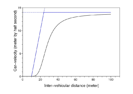
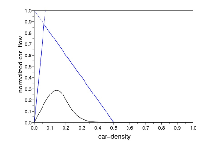
Figure 1: The effect of the stability condition $\alpha_{uw}\in[0,1]$ on the shape of the fundamental diagram.

Indeed, for the diagram (23), if we assume that $V_{e}$ is bounded by $v_{0}$, $V_{e}(y)=0,\forall y\in[0,y_{j}]$, and that $V_{e}$ is continuous (and increasing), then starting by the point $(y_{j},0)$, one cannot join any point above the line passing by $(y_{j},0)$ and having the slope $1$, with any sequence of segments of slopes $\alpha_{uw}\in[0,1]$. We can write

$$V_{e}(y)\leq\max(0,\min(v_{0},y-y_{0})).$$

Similarly, on the diagram (24), if we assume that $Q_{e}$ is continuous and $Q_{e}(\rho)=0,\forall\rho\in[\rho_{j},1]$, then going back from the point $(\rho_{j},0)$, one cannot attain any point above the line passing by $(\rho_{j},0)$ and $(0,1)$, with a sequence of segments having their ordinates at the origin ($\alpha_{uw})$ in $[0,1]$. We can write

$$Q_{e}(\rho)\leq\max(0,\min(v_{0}\rho,1-\rho/\rho_{j})).$$

3 Traffic on an open road

We study in this section the traffic on an open road with one lane and without passing. We are interested in the following dynamics.

$$\begin{array}[]{l}x_{1}(t+1)=x_{1}(t)+v_{1}(t),\\ x_{n}(t+1)=\min_{u\in\mathcal{U}}\max_{w\in\mathcal{W}}\{x_{n}(t)+\alpha_{uw}[x_{n-1}(t)-x_{n}(t)]+\beta_{uw}\}.\end{array}$$ (26)

If we denote by $M^{uw}$ the matrices

$$M^{uw}=\begin{bmatrix}1&0&\cdots&0\\ \alpha_{uw}&1-\alpha_{uw}&&0\\ \vdots&\ddots&\ddots&\\ 0&0&\alpha_{uw}&1-\alpha_{uw}\end{bmatrix},$$

and by $c^{uw}(t)$ the vectors

$$c^{uw}(t)={}^{t}[v_{1}(t),\;\;\beta_{uw},\;\cdots,\;\beta_{uw},\;\;\beta_{uw}],$$

for $(u,w)\in\mathcal{U}\times\mathcal{W}$ and $t\in\mathbb{N}$, then the dynamic system (26) is written

$$x_{n}(t+1)=\min_{u\in\mathcal{U}}\max_{w\in\mathcal{W}}\{[M^{uw}x(t)]_{n}+c^{uw}_{n}\},\quad 1\leq n\leq\nu\;.$$ (27)

It is easy to check that the dynamic system (27) is additive homogeneous of degree 1, and is monotone under the condition $\forall(u,w)\in\mathcal{U}\times\mathcal{W},\alpha_{uw}\in[0,1]$. Therefore, under that condition, (27) is non expansive. However, (27) is not connected for every $(u,w)\in\mathcal{U}\times\mathcal{W}$.

We will be interested here, in particular, in the stationary regime, where $v_{1}(t)$ reaches a fixed value $v_{1}$. For this case, the eigenvalue problem associated to (26) is

$$\begin{array}[]{l}\bar{v}+x_{1}=x_{1}+v_{1},\\ \bar{v}+x_{n}=\min_{u\in\mathcal{U}}\max_{w\in\mathcal{W}}\{x_{n}+\alpha_{uw}[x_{n-1}-x_{n}]+\beta_{uw}\}.\end{array}$$ (28)

The system (28) is also written

$$\bar{v}+x_{n}=\min_{u\in\mathcal{U}}\max_{w\in\mathcal{W}}\{[M^{uw}x]_{n}+c^{uw}_{n}\},\quad 1\leq n\leq\nu\;,$$ (29)

where

$$c^{uw}={}^{t}[v_{1},\;\;\beta_{uw},\;\cdots,\;\beta_{uw},\;\;\beta_{uw}].$$

Then we have the following result.

Theorem 3.

For all $y\in\mathbb{R}$ satisfying $\min_{u\in\mathcal{U}}\max_{w\in\mathcal{W}}(\alpha_{uw}y+\beta_{uw})=v_{1}$, the couple $(\bar{v},x)$ is a solution for the system (28), where $\bar{v}=v_{1}$ and $x$ is given up to an additive constant by

$$x={}^{t}[(n-1)y,\quad(n-2)y,\quad\cdots,\quad y,\quad 0].$$ (30)

Proof.

The proof is similar to that of Theorem 2. Let $y\in\mathbb{R}$ satisfying $\min_{u\in\mathcal{U}}\max_{w\in\mathcal{W}}(\alpha_{uw}y+\beta_{uw})=v_{1}$. Let $(\bar{u},\bar{w})\in\mathcal{U}\times\mathcal{W}$ such that $\alpha_{\bar{u}\bar{w}}y+\beta_{\bar{u}\bar{w}}=v_{1}$. Let $x$ be given by (30). Then $\forall n\in\{1,2,\cdots,\nu\}$ we have

$$[M^{\bar{u}\bar{w}}x]_{n}+c^{\bar{u}\bar{w}}_{n} =(\alpha_{\bar{u}\bar{w}}y+\beta_{\bar{u}\bar{w}})+x_{n}$$

$$=\min_{u\in\mathcal{U}}\max_{w\in\mathcal{W}}(\alpha_{uw}y+\beta_{uw})+x_{n}$$

$$=\min_{u\in\mathcal{U}}\max_{w\in\mathcal{W}}[M^{uw}x]_{n}+c^{uw}_{n}$$

$$=v_{1}+x_{n}.$$

∎

We can easily check that for $(u,w)\in\mathcal{U}\times\mathcal{W}$ such that $\alpha_{uw}=0$ and $\beta_{uw}=v_{1}$, every inter-vehicular distance $y\in\mathbb{R}$ satisfies the condition $\min_{u\in\mathcal{U}}\max_{w\in\mathcal{W}}(\alpha_{uw}y+\beta_{uw})=v_{1}$. Thus, such couples $(u,w)$ do not count for that condition. Theorem (3) can then be announced differently. Let us denote by $\mathcal{W}_{u}$ for $u\in\mathcal{U}$ the family of index sets

$$\mathcal{W}_{u}=\{w\in\mathcal{W},(\alpha_{uw},\beta_{uw})\neq(0,v_{1})\},$$

and by $\tilde{y}$ the asymptotic average car-inter-vehicular distance:

$$\tilde{y}=\max_{u\in\mathcal{U}}\min_{w\in\mathcal{W}_{u}}\frac{v_{1}-\beta_{uw}}{\alpha_{uw}},$$ (31)

where we use the convention $a/0=+\infty$ if $a>0$ and $a/0=-\infty$ if $a<0$. Then Theorem 3 tells simply that if $\tilde{y}\in\mathbb{R}$ (i.e. $-\infty<\tilde{y}<+\infty$), then the dynamic system (28) admits a solution $(\bar{v},x)$ where $\bar{v}=v_{1}$ is unique, and where $x$ is not necessarily unique and is given up to an additive constant by

$$x={}^{t}[(n-1)\tilde{y},\quad(n-2)\tilde{y},\quad\cdots,\quad\tilde{y},\quad 0].$$

Non-uniform asymptotic car-distributions can also be obtained. Let us clarify the following three cases.

• If $\exists u\in\mathcal{U},\forall w\in\mathcal{W}_{u},\alpha_{uw}=0$ and $\beta_{uw}<v_{1}$, then $\tilde{y}=+\infty$. In this case, the distance between the first car and the other cars increases over time and goes to $+\infty$. The asymptotic car-distribution on the road is not uniform.

• If $\forall u\in\mathcal{U},\exists w\in\mathcal{W}_{u},\alpha_{uw}=0$ and $\beta_{uw}>v_{1}$, then $\tilde{y}=-\infty$. In this case, the first car is passed by all other cars, and the distance between the first car and the other cars increases over time and goes to $+\infty$. The asymptotic car-distribution on the road is not uniform.

• If $\forall u\in\mathcal{U},\forall w\in\mathcal{W}_{u},\alpha_{uw}=0$ and if $\min_{u\in\mathcal{U}}\max_{w\in\mathcal{W}_{u}}\beta_{uw}=v_{1}$, then for all $x\in\mathbb{R}^{\nu}$, $(v_{1},x)$ is a solution for the system (28). In this case, every distribution of the cars moving all with the constant velocity $v_{1}$ is stationary.

The formula (31) is the fundamental traffic diagram expressing the average inter-vehicular distance as a function of the car speed at the stationary regime. In the case where only a minimum operator is used in (26), the formula (31) is reduced to the convex fundamental diagram

$$y=\max_{u\in\mathcal{U}}\frac{v_{1}-\beta_{u}}{\alpha_{u}}.$$ (32)

Example 1.

In order to understand the transient traffic, let us simulate the car-dynamics (26). We take as the time unit half a second (1/2 s), and as the distance unit 1 meter (m). The parameters of the model are determined by approximating the behavior law (6), with a free velocity $v_{0}=14$ m/ 1/2s (which is about 100 km/h) and $\gamma=7.5$ as in [25]; see Figure 2.

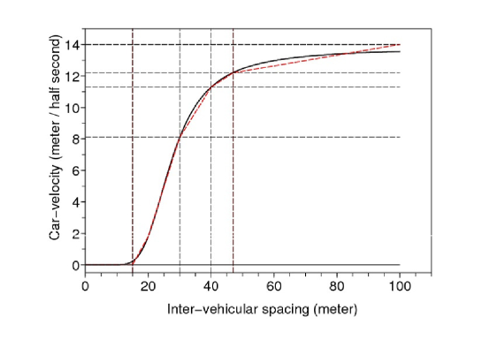
Figure 2: Approximation of the behavioral law (6) with a piecewise linear curve.

The behavior law is approximated by the following piecewise linear curve of six segments.

$$\tilde{V}(y)=\max\{\alpha_{1}y+\beta_{1},\min\{\alpha_{2}y+\beta_{2},\alpha_{3}y+\beta_{3},\alpha_{4}y+\beta_{4},\alpha_{5}y+\beta_{5},\alpha_{6}y+\beta_{6}\}\},$$

where the parameters $\alpha_{i}$ and $\beta_{i}$ for $i=1,2,\cdots,6$ are given by

Segments	1	2	3	4	5	6
$\alpha_{i}$	0	0.54	0.32	0.13	0.34	0
$\beta_{i}$	0	-8.1	-1.47	6.11	10.6	14

We simulate the piecewise linear car-following model associated to the approximation above.

$$\begin{array}[]{l}x_{1}(t)=x_{1}(t-1)+v_{1}(t),\\ x_{n}(t)=x_{n}(t-1)+\tilde{V}(x_{n-1}(t-1)-x_{n}(t-1)).\end{array}$$ (33)

The velocity of the first car $v_{1}(t),t\geq 0$ is varied in the time interval $[0,1000]$, then fixed to the free velocity $v_{0}=14$ m/ 1/2s in the time interval $[1000,3000]$, and finally fixed on a velocity that exceeds $v_{0}$ in the remaining time $[3000,7200]$. The average inter-vehicular distance is then computed at every time $t$, and the results are shown in Figure 3.

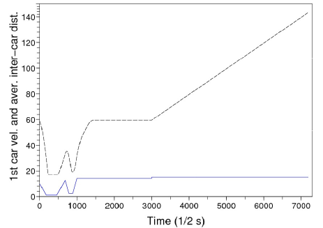
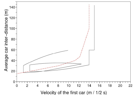
Figure 3: Simulation results. On the left-side: the first car velocity (solid line), and the average inter-vehicular distance (dash line) functions of time. On the right side: the approximation of the behavior law (6) (dash line), and the average inter-vehicular distance obtained by simulation in function of the velocity of the first car (solid line).

The simple simulation we made here permits to have an idea of the traffic in the transient regime. Figure 3 shows how the average of the inter-vehicular distance is changed due to a changing in the velocity of the first car. In the right side of Figure 3, we compare the fundamental law assumed in the model with the diagram giving the average inter-vehicular distance (with respect to the number of cars) function of the velocity of the first car (a kind of macroscopic fundamental diagram). We observe that loops are obtained on that diagram in the transient traffic. The loops are interpreted by the fact that once the velocity of the first car is temporarily stationary, the velocities of the following cars, and thus also the average velocity of the cars, make some time to attain the first car velocity. It can also be interpreted by saying that even though the cars have, individually, the same response to a changing in inter-vehicular distance; their collective response depends on whether the inter-vehicular distance is increasing or decreasing. The apparition of such loops is due to the reaction time of drivers. It can also be related to the number of anticipation cars in case of multi-anticipative modeling. However, one may measure on a given section, different car-flows for the same car density (or occupancy rate) depending on the traffic acceleration or deceleration, and interpret it as the hysteresis phenomenon [8, 31, 32, 15].

4 Conclusion

We proposed in this article a car-following model which extends the linear car-following model as well as the min-plus model. The stability and the stationary regimes of the model are characterized thanks to a variational formulation of the car-dynamics. This formulation, although already made with continuous-time models, it permits to clarify the stimulus-response process in microscopic discrete-time traffic models, and to interpret it in term of stochastic optimal control. Among the important questions to be treated in the future, the impacts of heterogeneity and anticipation in driving, on the transient and stationary traffic regimes, based on the model proposed in this article.

Appendix A Connectedness of system (14)

Let $x\in\mathbb{R}^{\nu}$. We denote by $h:\mathbb{R}^{\nu}\to\mathbb{R}^{\nu}$ the operator defined by $h(x(t))=x(t+1)$, where $x_{n}(t+1)$, for $1\leq n\leq\nu$ are given by the definition of the system (14). That is

$$x_{n}(t+1)=\min_{u\in\mathcal{U}}\{[M^{u}x(t)]_{n}+c^{u}_{n}\},\quad 1\leq n\leq\nu\;.$$

• If $\exists u\in\mathcal{U}$, such that $\alpha_{u}\in(0,1]$, then for all $n\in\{1,2,\cdots,\nu\}$, there exists an arc, on the graph associated to $h$, going from $n-1$ to $n$ ($n$ being cyclic in $\{1,2,\cdots,\nu\}$). Indeed,

  $$x_{n}(t+1)=(1-\alpha_{u})x_{n}(t)+\alpha_{u}x_{n-1}(t)+\beta_{u}.$$

  Then since $\alpha_{u}>0$, we get:

  $$\lim_{\nu\to\infty}h_{n}(\nu e_{n-1})=\lim_{\nu\to\infty}[\alpha_{u}\nu+\beta_{u}]=\infty.$$

  where $e_{n-1}$ denotes the $(n-1)^{th}$ vector of the canonic basis of $\mathbb{R}^{\nu}$. Therefore the graph associated to $h$ is strongly connected.

• If $\forall u\in\mathcal{U},\alpha_{u}=0$, then we can easily check that all arcs of the graph associated to $h$ are loops. Hence that graph is not strongly connected.

Appendix B Duality in traffic modeling

We show in this appendix the duality in traffic modeling of using the three functions

• $n(t,x)$: cumulated number of cars passed through position $x$ from time $0$ up to time $t$.

• $x(n,t)$: position of car $n$ at time $t$ (or cumulated traveled distance of car $n$ from time $0$ up to time $t$).

• $t(n,x)$: the time that car $n$ passes by position $x$.

We base on the Lagrangian traffic descriptions given in the introduction, and give the equivalent traffic descriptions by using the functions $n(t,x)$ and $t(n,x)$, in both cases of discrete-time and continuous-time modeling.

1. In Eulerian traffic descriptions, the function $n(t,x)$ is used. The partial derivative $\partial_{t}n(t,x)$ expresses the car-flow $q(t,x)$ at time $t$ and position $x$, while $-\partial_{x}n(t,x)$ expresses the car-density $\rho(t,x)$ at time $t$ and position $x$. The equality $\partial_{tx}n(t,x)=\partial_{xt}n(t,x)$ gives the car conservative law:

   $$\partial_{t}k(t,x)+\partial_{x}q(t,x)=0.$$ (34)

   The first order traffic model LWR [26, 29] supposes the existence of a fundamental diagram of traffic giving the car-flow $q$ as a function of the car-density $\rho$ at the stationary regime, through a function $Q_{e}$, and that the diagram also holds for the transient traffic :

   $$q(t,x)=Q_{e}(\rho(t,x)).$$ (35)

   Then (34) and (35) give the well known LWR model

   $$\partial_{t}\rho(t,x)+\partial_{x}\rho(t,x)Q_{e}^{\prime}(\rho)=0.$$ (36)

   Also discrete-time and -space Eulerian traffic models exist. Those models are in general derived from Petri nets as in [2, 10, 9]. For example the traffic on a 1-lane road without passing can be described by

   $$n(t,x)=\min\{a_{x}+n(t-\tau_{x},x-\delta x),\quad\bar{a}_{x+\delta x}+n(t-\bar{\tau}_{x+\delta x},x+\delta x)\},$$ (37)

   where

   • denotes the number of cars being in $(x-\delta x,x)$ at time zero.

   • denotes the free travel-time of a car from $x-\delta x$ to $x$.

   • denotes the space non occupied by cars in $(x-\delta x,x)$ at time zero. If we denote by $c_{x}$ the maximum number of cars that can be in $(x-\delta x,x)$, then we have simply $\bar{a}_{x}=c_{x}-a_{x}$.

   • denotes the reaction time of drivers in $(x-\delta x,x)$. That is the time interval between the time when $(x-\delta x,x)$ is free of cars and the time when a car being in $(x-2\delta x,x-\delta x)$ starts moving to $(x-\delta x,x)$. If we denote by $T_{x}$ the total traveling time (reaction time + moving time) of a car from $(x-2\delta x,x-\delta x)$ to $(x-\delta x,x)$, then we have simply $\bar{\tau}_{x}=T_{x}-\tau_{x}$.

2. By using the variable $t(n,x)$, the first order differentiation of $t(n,x)$ with respect to $n$, denoted $z$ is $z(n,x)=-(t(n-1,x)-t(n,x))$, while the derivative of $t(n,x)$ in $x$, denoted $r$ is $r(n,x)=\partial_{x}t(n,x)$. We notice here that $z$ and $r$ are interpreted respectively as the inverse flow and the inverse velocity of vehicles. A conservation law (of time) is then written

   $$\partial_{x}z(n,x)+r(n,x)-r(n-1,x)=0.$$ (38)

   The law (38) combined with the fundamental diagram $r=R_{e}(z)$ gives the model

   $$\partial_{x}r(n,x)=R^{\prime}(z(n,x))\Delta r(n,x),$$ (39)

   where $\Delta r(n,x)=r(n-1,x)-r(n,x)$. Note that, having a fundamental diagram $v=V_{e}(q)$ giving the stationary velocity as a function of the stationary flow, the diagram $R_{e}$ is nothing but $R_{e}(z)=1/V_{e}(1/z)$.

   Discrete-time-and-space modeling with the function $t(n,x)$ also exist. The models are also inspired from Petri net, and dual dynamics to (37) are obtained. For example, using the same notations as in (37), the traffic on a 1-lane road without passing can be described by

   $$t(n,x)=\max\{\tau_{x}+t(n-a_{x},x-\delta x),\;\bar{\tau}_{x+\delta x}+t(n+\bar{a}_{x+\delta x},x+\delta x)\}.$$ (40)

   Note here that a max operator is used rather than a min one. For more details on the duality of (37) and (40) and the meanings in term of Petri nets, event graphs and min-plus or max-plus algebras, see [2].

References

- [1] Jean-Pierre Aubin, Alexandre M. Bayen, and Patrick Saint-Pierre. Dirichlet problems for some hamilton-jacobi equations with inequality constraints. Siam Journal on Control and Optimization, 47:1218–1222, 2009.
- [2] F. Baccelli, G. Cohen, G.-J. Olsder, and J.-P. Quadrat. Synchronization and Linearity. Wiley, 1992.
- [3] M. Bando, K. Hasebe, A. Nakayama, A. Shibata, and Y. Sugiyama. Dynamical model of traffic congestion and numerical simulation. Physical Review E, 51(2), 1995.
- [4] M.G. Candrall and L. Tartar. Some relations between nonexpansive and order preserving mappings. Proceedings of the American Mathematical Society, 78(3):385–390, 1980.
- [5] R. E. Chandler, R. Herman, and E. W. Montroll. Traffic dynamics: Studies in car following. Operations Research, 6:165–184, 1958.
- [6] Carlos F. Daganzo. On the variational theory of traffic flow: well-posedness, duality and applications, networks and heterogeneous media 1(4, 2006.
- [7] Carlos F. Daganzo and Nikolas Geroliminis. An analytical approximation for the macroscopic fundamental diagram of urban traffic. Transportation Research Part B: Methodological, 42(9):771–781, November 2008.
- [8] Leslie C. Edie. Car-Following and Steady-State Theory for Noncongested Traffic. Operations Research, 9(1):66–76, 1961.
- [9] N. Farhi, M. Goursat, and J.-P. Quadrat. The traffic phases of road networks. Transportation Research Part C, 19(1):85–102, 2011.
- [10] Nadir Farhi. Modélisation Minplus et Commande du Trafic de Villes Régulières. PhD thesis, Université Paris 1 Panthéon-Sorbonne, 2008.
- [11] S. Gaubert and J. Gunawardena. A non-linear hierarchy for discrete event dynamical systems. In Proceedings of WODES’98, Cagliari, Italia, 1998.
- [12] S. Gaubert and J. Gunawardena. Existence of eigenvectors for monotone homogeneous functions. Hewlett-Packard Technical Report, pages HPL–BRIMS–99–08, 1999.
- [13] D C Gazis, R Herman, and R W Rothery. Nonlinear follow-the-leader models of traffic flow. Operations Research, 9(4):545–567, 1961.
- [14] Denos C. Gazis, Robert Herman, and Renfrey B. Potts. Car-Following Theory of Steady-State Traffic Flow. Operations Research, 7(4):499–505, 1959.
- [15] Nikolas Geroliminis and Jie Sun. Hysteresis phenomena of a macroscopic fundamental diagram in freeway networks. Transportation Research Part A: Policy and Practice, 2011.
- [16] H. Greenber. An analysis of traffic flow. Operations research, 7, 1959.
- [17] B. D. Greenshields. A study of traffic capacity. Proc. Highway Res. Board, 14:448–477, 1935.
- [18] J. Gunawardena and M. Keane. On the existence of cycle times for some nonexpansive maps. Hewlett-Packard Technical Report, pages HPL–BRIMS–95–003, 1995.
- [19] W. Helly. Simulation of bottlenecks in single lane traffic flow. In International Symposium on the Theory of Traffic Flow, 1959.
- [20] W. Helly. Simulation of bottlenecks in single lane traffic flow. in theory of traffic flow. Elsevier Publishing Co., pages 207–238, 1961.
- [21] R Herman, E W Montroll, R B Potts, and R W Rothery. Traffic dynamics: Analysis of stability in car following. Operations Research, 7(1):86–106, 1959.
- [22] M HERRMANN and B KERNER. Local cluster effect in different traffic flow models. Physica A-statistical Mechanics and Its Applications, 255:163–188, 1998.
- [23] Serge P Hoogendoorn, Saskia Ossen, and M Schreuder. Empirics of multianticipative car-following behavior. Transportation Research Record, 1965:112–120, 2006.
- [24] B. S. Kerner and P. Konhäuser. Cluster effect in initially homogeneous traffic flow. Phys. Rev. E, 48(4):R2335–R2338, Oct 1993.
- [25] H. Lenz, C. K. Wagner, and R. Sollacher. Multi-anticipative car-following model. European Physical Journal B, 7:331–335, 1999.
- [26] J. Lighthill and J. B. Whitham. A min-plus derivation of the fundamental car-traffic law. Proc. Royal Society, A229:281–345, 1955.
- [27] Pablo Lotito, Elina Mancinelli, and Jean-Pierre Quadrat. A min-plus derivation of the fundamental car-traffic law. IEEE Transactions on Automatic Control, 50:699–705, 2005.
- [28] G. F. Newell. Nonlinear effects in the dynamics of car following. Operations research, 9(2):209–229, 1961.
- [29] P. I. Richards. Shock waves on the highway. Operations Research, 4:42–51, 1956.
- [30] Martin Treiber, Ansgar Hennecke, and Dirk Helbing. Congested traffic states in empirical observations and microscopic simulations. PHYSICAL REVIEW E, 62:1805, 2000.
- [31] J. Treiterer and J.A. Myers. The hysteresis phenomena in traffic flow. In Proceedings of the sixth symposium on transportation and traffic theory, pages 13–38, 1974.
- [32] H. M. Zhang. A mathematical theory of traffic hysteresis. Transportation Research Part B: Methodological, 33(1):1–23, February 1999.