Measurement and Application of Entropy Production Rate
in Human Subject Social Interaction Systems

Abstract

This paper illustrates the measurement and the applications of the observable, entropy production rate (EPR), in human subject social interaction systems. To this end, we show (1) how to test the minimax randomization model with experimental 2$\times$2 games data and with the Wimbledon Tennis data; (2) how to identify the Edgeworth price cycle in experimental market data; and (3) the relationship within EPR and motion in data. As a result, in human subject social interaction systems, EPR can be measured practically and can be employed to test models and to search for facts efficiently.

I Introduction

Laboratory experiment in human subject social interaction systems (HSSIS) has becoming major tool for fundamentally social science Falk and Heckman (2009); Plott and Smith (2008), in which developing signature observable is meaningful.

Entropy and entropy production rate (EPR), a twin observable, correspond to the diversity and the activity of a system Andrae et al. (2010); Zia and Schmittmann (2007), respectively. In game theory for HSSIS, entropy has been noticed theoretically Grunwald and Dawid (2004) and experimentally Bednar et al. (2011); Cason et al. (2009). Denoting the density of state (DOS) as $P_{i}$ for state $i$ ($i\in X$ and $X$$:=\{1,2,...,r\}$ is the full social strategy set), the entropy $S$ is as Bednar et al. (2011),

$$S=-\sum_{i}P_{i}\log_{r}P_{i}.$$ (1)

In games, entropy can identify the distribution in $X$ and the diversity of HSSIS Bednar et al. (2011); Cason et al. (2009). EPR serves as a central observable for the activity of many natural systems Andrae et al. (2010), however, in HSSIS, EPR has never been reported empirically; Developing EPR as an observable in HSSIS is the main aim of this letter.

As the discrete Markov chains can be obtained Cason et al. (2005); Buchheit and Feltovich (2011) in HSSIS, the metric for EPR could borrow from physics Gaspard (2004); Maes and Neto ny (2003); Andrae et al. (2010). For a system with small number of states and lasting time long enough, the stationary state approximation can be considered Selten and Chmura (2008); the associated mean entropy production rate $\dot{S}$ (EPR) is as Gaspard (2004); Maes et al. (2011); Dorosz and Pleimling (2011); Andrae et al. (2010)

$$\dot{S}=\frac{1}{2}\sum_{i,j}\left[P_{i}\omega_{ij}-P_{j}\omega_{ji}\right]\log_{r}\left[\frac{P_{i}\omega_{ij}}{P_{j}\omega_{ji}}\right],$$ (2)

in which $P_{i}$ is the DOS and $\omega_{ij}$ is the transition probability from state $i$ to $j$. Fig. 1(c) is an empirical example for $P_{i}$, $\omega_{ij}$ and a Markovian.

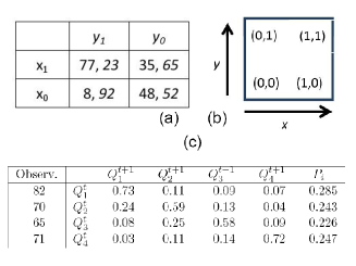
Figure 1: (a, b) a payoff matrix and the strategy space $X$ (2$\times$2 game, Trt. 31 in Table 1); (c) a Markovian with $\omega_{ij}$ and $P_{i}$ (from top-left subtable in Table 1 in ref. Cason et al. (2005), also Trt. 48 in Table 1); in (c), the entropy is 0.9952 and the EPR is 0.0481.

Table 1: Empirical Data from HSSIS

Game	Trt.	States	Rec./Trt.	Ref.
2$\times$2	31-40	4	4500	Erev et al. (2007)
2$\times$2	41	4	$\sim$3600	MP4
WT(2$\times$2)	45-47	4	$\sim$2000	Hsu et al. (2007)
EC	48-55	4	$\sim$200	Cason et al. (2005)
HS(2$\times$2)	56-57	4	2600	Rosenthal et al. (2003)

The data is collected from the published 24 experimental economics treatments (EET) listed in Table 1. All of the 24 EET, the state number ($r$) is 4. Each of the EET is of an unique mixed strategy Nash equilibrium and of long rounds satisfying the stationary approximation Selten and Chmura (2008). These are practically the simplest systems for EPR . For more details, see Appendix.

To demonstrate the EPR’s applications, the paper is as follows, (1) testing an economics model with EPR; (2) detecting an economics phenomena with EPR; and (3) verifying a relationship within two dynamical variables with EPR; Then, summary last.

II EPR and Radomization in Minimax

The von Neumann’s Minimax model (vNM) ’represents game theory in its most elegant form: simple but with stark predictions’ Levitt et al. (2010). In vNM, playing mixed strategy game ’against an at least moderately intelligent opponent’, should be ’playing irregularly heads and tails in successive games’ (the randomization prediction), except that the possibility of a strategy used is constrained. The randomization prediction of vNM is tested with EPR.

In Fig. 2, the entropy and EPR from the 16 EET of the 2$\times$2 games (Trt. 31-41, 45-47 and 56-57) are shown (in $\bullet$ or $\blacktriangle$).

The vNM randomization predictions can be realized directly with simple Monte Carlo simulation (MCs) Palacios Huerta (2003). We conduct the MCs $10^{4}$ times for each of the 16 EET, respectively; For a MCs, there are two constrains: First, holds the same sample size of sessions, rounds and agents as its related EET; Second, holds the same mean strategy possibility as its related EET . As results of the vNM randomization prediction, the entropy and EPR  are shown (in $\circ$ or $\vartriangle$) in Fig. 2.

Comparing entropy and EPR values from the vNM and from the HSSIS respectively, we have (1) the vNM can not be rejected with the entropy comparison ; But, (2) the EPR values from HSSIS is significant larger than that from vNM ($p$$<$0.001, 16 samples, $t-test$ ). With EPR, the randomization prediction of vNM have to be rejected.

It is an example of testing a behavior model with EPR.

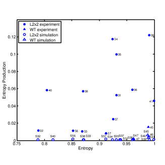
Figure 2: Obtained entropy (in horizon) and and EPR (in vertical) in the 2$\times$2 games. Experimental results of the Trt. ID in Table 1 labels in solid. The result of mean entropy and EPR from the $10^{4}$ times vNMs are in hole and labeled start with ’S’ and the Trt. ID.

III EPR and Edgeworth Cycle

Many years ago, Edgeworth predicted persistent price cycles phenomena in a competitive situation where the only equilibrium is in mixed strategies Benaīm et al. (2009); Maskin and Tirole (1988). It is very puzzling because it seemingly contradicts the law of one price of elementary microeconomics Lahkar (2007). The cycles, e.g., in retail gasoline markets Noel (2007), have been obtained in real economies; meanwhile, the welfare effects of the cycles have been found Noel (2011). Usually, detecting the cycle is uneasy Benaīm et al. (2009); Cason et al. (2005).

In a stationary state, if the EPR systematically deviates from zero, there must be balanced cycle fluxes, and this is a simple consequence of Kirchhoff’s Law Gaspard (2004); Qian and Beard (2005). Meanwhile, in a finite dataset, as Trt. 48-55, the obtained EPR can be the bias from finite sample (e.g., Schourmann (2004)). To correct the bias, we use the EPR from repeated MCs as base line zero (denoted as $B^{0}$). So the existence of a cycle in a EET can be simplified to a sharp testable hypothesis (H0): for the $i$-th EET, the empirical $EPR_{i}$ equals to the $B^{0}_{i}$.

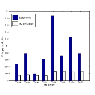
Figure 3: EPR in the price dispersion market game from the data of the laboratory experiments (solid bar) and Monte Carlo simulations (blank bar, mean value of $B^{0}_{i}$, $10^{4}$ times repeated, see text), respectively.

In Fig. 3, each of the empirical EPR_i of the 8 EET (Trt. 48-55) is shown in solid bar and the $B^{0}_{i}$ is in blank bar. Each $B^{0}_{i}$ comes from the MCs with the constraint of the price distribution from the Markovian and the number of rounds as its related EET. As a result, in 7 EET (except Trt. 50), the empirical EPR_i is larger significant than its $B^{0}_{i}$ ($p<0.001$) . So, the existence of Edgeworth cycle in each of the 7 EET can be supported efficiently .

It is an example of detecting an economic phenomena with EPR.

IV EPR and Motion

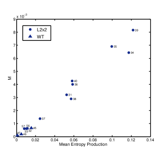
Figure 4: Empirical relationship of the motion (M) and EPR in the EET of the 2$\times$2 games. Labels relate to the Trt. ID in Table 1

In evolutionary game theory, an evolutionary dynamic equation describes the velocity of evolution in space $X$ Altrock and Traulsen (2009); Weibull (1997); Bowles (2004); Sigmund (2010). Experimental economics is a test bed for evolutionary game theory Crawford (1991); Binmore et al. (1993); Samuelson (2002); Van Huyck et al. (1995); Binmore et al. (2001); Battalio et al. (2001); Cason et al. (2005); Bouchez and Friedman (2008), and recently the velocity patterns in strategy space are observed Xu and Wang (2011b, a). As both of the observables, the velocity in Eq.(4) and the EPR in Eq.(2), describe the time reversal asymmetry processes of experimental social dynamics  Zia and Schmittmann (2007); Xu and Wang (2011b); Baiesi et al. (2009); Castellano and Loreto (2009), the relationship within them is natural concerned.

Fig. 4 is the scattering of the motion ($M$) and EPR of the 16 EET (Trt. 31-41, 45-47 and 56-57, the 2$\times$2 games). Here, the motion ($M$) is defined as,

$$M=\frac{1}{2}\sum_{i\alpha}P_{i}v_{i\alpha}^{2},$$ (3)

in which, $P_{i}$ is the DOS of $i$ ($i\in\mathbf{S}$) and $\alpha$ denotes the two dimensions of movements in a two-population 2$\times$2 games as in Fig. 1(b). The velocity Xu and Wang (2011b, a), $v_{i\alpha}$, in Markovian format is

$$v_{i\alpha}=\sum_{j}\left[(P_{j}\omega_{ji}-P_{i}\omega_{ij})(x_{i\alpha}-x_{j\alpha})\right],$$ (4)

in which $x_{i\alpha}$ is the vector of the $\alpha$ companion of the $i$ state in Euclidean $X$  Xu and Wang (2011b, a). Denoting the EPR as $P$, the simple linear fit (OLE) results: $M$=($0.064\pm$0.003)$P$ + $0.000$ and $R^{2}=0.97$ for the 16 EET.

As an empirical finding, the motion ($M$) is positive and linear dependent on the EPR in the data.

V Summary and outlook

There is no reason that the approach to predicting the behavior of physical systems is not appropriate when the physical system in question is some human beings playing a game Wolpert (2010). EPR is one of the key signatures of non-equilibrium steady (stationary) states Zia and Schmittmann (2007) and we link EPR to the stationary state Selten and Chmura (2008) of HSSIS. The potential advantage of the EPR observable should be:

(1) At speaking to theorists Roth (2010): The EPR could serve as an independent variable to test behavior models. For example, testing the randomization prediction of vNM is hard  O’Neill (1987); Brown and Rosenthal (1990); Binmore et al. (2001); Walker and Wooders (2001); Shachat (2002); Chiappori et al. (2002); Levitt et al. (2010), as we have shown above, EPR is effective for the task. Whether models Erev et al. (2010); Selten and Chmura (2008) can be verified with EPR is becoming a question.

(2) At searching for facts Roth (2010): (a) EPR could serve as a variable to detect the heterogeneous of behavior, e.g. in Wimbledon Tennis Hsu et al. (2007), the EPR in the juniors, females and males are significant different. (b) the EPR could detect the dynamical pattern. With the time reversal symmetry (asymmetry) consideration, unifying themes for the phenomena like Edgeworth cycle, Shapley polygon Shapley (1964), and the Scarf price dynamics on Walrasian general equilibrium Anderson et al. (2004); Gintis (2007) can be expected.

(3) At Bridging between physics and economics: Since 1990s Evans et al. (1993), the physics near stationary (or steady, equilibrium) state is becoming fruitful Maes and Neto ny (2003); Gaspard (2004); Zia and Schmittmann (2007); Dorosz and Pleimling (2011); Maes et al. (2011). This paper is benefit from the physics. Meanwhile, the empirical results of EPR and the methods here could feedback to the developing physics, e.g., to verify the relations of the observable (and variables). In social dynamics Castellano and Loreto (2009), with dynamical observable likes EPR, excellent developments could be expected.

In summary, firstly and empirically in HSSIS, this paper has illustrated function of the observable, EPR, on models testing and facts finding, which could benefit to the both, physics and economics.

Our outlook is, as in physics, EPR can be a signature observable in the human subject social interaction systems.

Notes: We thanks Ken Binmore and Al Roth for helpful discussion and the data providing. The programmes for the Monte Carlo simulations and statistical analysis, the primary data set and the instructions of our laboratory experiment MP4 in Table 1 are available from the authors website.

References

- Falk and Heckman (2009) A. Falk and J. Heckman, Science 326, 535 (2009).
- Plott and Smith (2008) C. Plott and V. Smith, Handbook of experimental economics results (North-Holland, 2008).
- Andrae et al. (2010) B. Andrae, J. Cremer, T. Reichenbach, and E. Frey, Physical review letters 104, 218102 (2010).
- Zia and Schmittmann (2007) R. Zia and B. Schmittmann, Journal of Statistical Mechanics: Theory and Experiment 2007, P07012 (2007).
- Grunwald and Dawid (2004) P. Grunwald and A. Dawid, the Annals of Statistics 32, 1367 (2004).
- Bednar et al. (2011) J. Bednar, Y. Chen, T. Liu, and S. Page, Tech. Rep., Mimeo, University of Michigan (2011).
- Cason et al. (2009) T. Cason, A. Savikhin, and R. Sheremeta, Cooperation Spillovers in Coordination Games (2009).
- Cason et al. (2005) T. Cason, D. Friedman, and F. Wagener, Journal of Economic Dynamics and Control 29, 801 (2005), ISSN 0165-1889.
- Buchheit and Feltovich (2011) S. Buchheit and N. Feltovich, International Economic Review 52, 317 (2011).
- Gaspard (2004) P. Gaspard, Journal of statistical physics 117, 599 (2004).
- Maes and Neto ny (2003) C. Maes and K. Neto ny, Journal of statistical physics 110, 269 (2003).
- Selten and Chmura (2008) R. Selten and T. Chmura, The American Economic Review 98, 938 (2008).
- Maes et al. (2011) C. Maes, Netoccaronn, yacute, Karel, and B. Wynants, Physical review letters 107, 010601 (2011).
- Dorosz and Pleimling (2011) S. Dorosz and M. Pleimling, Physical Review E 84, 011115 (2011).
- Hsu et al. (2007) S. Hsu, C. Huang, and C. Tang, The American Economic Review 97, 517 (2007).
- Rosenthal et al. (2003) R. Rosenthal, J. Shachat, and M. Walker, International Journal of Game Theory 32, 273 (2003).
- Xu and Wang (2011a) B. Xu and Z. Wang, Arxiv preprint arXiv:1105.3433 (2011a).
- Erev et al. (2007) I. Erev, A. Roth, R. Slonim, and G. Barron, Economic Theory 33, 29 (2007).
- Levitt et al. (2010) S. Levitt, J. List, and D. Reiley, Econometrica 78, 1413 (2010).
- Palacios Huerta (2003) I. Palacios Huerta, Review of Economic Studies 70, 395 (2003).
- Benaīm et al. (2009) M. Benaīm, J. Hofbauer, and E. Hopkins, Journal of Economic Theory 144, 1694 (2009), ISSN 0022-0531.
- Maskin and Tirole (1988) E. Maskin and J. Tirole, Econometrica 56, 571 (1988).
- Lahkar (2007) R. Lahkar, The dynamic instability of dispersed price equilibria (2007).
- Noel (2007) M. Noel, The Review of Economics and Statistics 89, 324 (2007).
- Noel (2011) M. Noel, EDGEWORTH PRICE CYCLES, New Palgrave Dictionary of Economics, forthcoming (2011).
- Qian and Beard (2005) H. Qian and D. Beard, Biophysical chemistry 114, 213 (2005).
- Schourmann (2004) T. Schourmann, Journal of Physics A: Mathematical and General 37, L295 (2004).
- Altrock and Traulsen (2009) P. Altrock and A. Traulsen, Physical Review E 80, 011909 (2009).
- Weibull (1997) J. Weibull, Evolutionary game theory (The MIT press, 1997).
- Bowles (2004) S. Bowles, Microeconomics: behavior, institutions, and evolution (Princeton University Press, 2004).
- Sigmund (2010) K. Sigmund, The calculus of selfishness (Princeton Univ Pr, 2010).
- Crawford (1991) V. Crawford, Games and Economic Behavior 3, 25 (1991).
- Binmore et al. (1993) K. Binmore, J. Swierzbinski, S. Hsu, and C. Proulx, International Journal of Game Theory 22, 381 (1993).
- Samuelson (2002) L. Samuelson, The Journal of Economic Perspectives 16, 47 (2002).
- Van Huyck et al. (1995) J. Van Huyck, R. Battalio, S. Mathur, P. Van Huyck, and A. Ortmann, International Journal of Game Theory 24, 187 (1995).
- Binmore et al. (2001) K. Binmore, J. Swierzbinski, and C. Proulx, The Economic Journal 111, 445 (2001).
- Battalio et al. (2001) R. Battalio, L. Samuelson, and J. Van Huyck, Econometrica 69, 749 (2001).
- Bouchez and Friedman (2008) N. Bouchez and D. Friedman, Handbook of Experimental Economics Results 1, 472 (2008).
- Xu and Wang (2011b) B. Xu and Z. Wang, Evolutionary Dynamical Pattern of ”Coyness and Philandering”: Evidence from Experimental Economics, vol. 3 (p1313-1326, NECSI Knowledge Press, ISBN 978-0-9656328-4-3., 2011b).
- Baiesi et al. (2009) M. Baiesi, C. Maes, and B. Wynants, Journal of statistical physics 137, 1094 (2009).
- Castellano and Loreto (2009) C. Castellano and V. Loreto, Reviews of Modern Physics 81, 591 (2009).
- Wolpert (2010) D. Wolpert, NASA Ames Research Center (2010).
- Roth (2010) A. Roth, The Methods of Modern Experimental Economics, Oxford University Press (2010).
- O’Neill (1987) B. O’Neill, Proceedings of the National Academy of Sciences of the United States of America 84, 2106 (1987).
- Brown and Rosenthal (1990) J. Brown and R. Rosenthal, Econometrica 58, 1065 (1990).
- Walker and Wooders (2001) M. Walker and J. Wooders, The American Economic Review 91, 1521 (2001).
- Shachat (2002) J. Shachat, Journal of Economic Theory 104, 189 (2002).
- Chiappori et al. (2002) P. Chiappori, S. Levitt, and T. Groseclose, American Economic Review pp. 1138–1151 (2002).
- Erev et al. (2010) I. Erev, E. Ert, A. Roth, E. Haruvy, S. Herzog, R. Hau, R. Hertwig, T. Stewart, R. West, and C. Lebiere, Journal of Behavioral Decision Making 23, 15 (2010).
- Shapley (1964) L. Shapley, Advances in game theory 52, 1¨C29 (1964).
- Anderson et al. (2004) C. Anderson, C. Plott, K. Shimomura, and S. Granat, Journal of Economic Theory 115, 209 (2004).
- Gintis (2007) H. Gintis, The Economic Journal 117, 1280 (2007).
- Evans et al. (1993) D. J. Evans, E. G. D. Cohen, and G. P. Morriss, Physical review letters 71, 2401 (1993).