Reconstructing Isoform Graphs from RNA-Seq data

Abstract

Next-generation sequencing (NGS) technologies allow new methodologies for alternative splicing (AS) analysis. Current computational methods for AS from NGS data are mainly focused on predicting splice site junctions or de novo assembly of full-length transcripts. These methods are computationally expensive and produce a huge number of full-length transcripts or splice junctions, spanning the whole genome of organisms. Thus summarizing such data into the different gene structures and AS events of the expressed genes is an hard task.

To face this issue in this paper we investigate the computational problem of reconstructing from NGS data, in absence of the genome, a gene structure for each gene that is represented by the isoform graph: we introduce such graph and we show that it uniquely summarizes the gene transcripts. We define the computational problem of reconstructing the isoform graph and provide some conditions that must be met to allow such reconstruction. Finally, we describe an efficient algorithmic approach to solve this problem, validating our approach with both a theoretical and an experimental analysis.

1 Introduction

Next-generation sequencing (NGS) technologies allow massive and parallel sequencing of biological molecules (DNA and RNA), and have a huge impact on molecular biology and bioinformatics [1]. In particular, RNA-Seq is a recent technique to sequence expressed transcripts, characterizing both the type and the quantity of transcripts expressed in a cell (its transcriptome). Challenging tasks of transcriptome analysis via RNA-Seq data analysis  [2, 3, 4] are reconstructing full-length transcripts (or isoforms) of genes and their expression levels. The most recent studies indicate that alternative splicing is a major mechanism generating functional diversity in humans and vertebrates, as at least 90% of human genes exhibit splicing variants. The annotation of alternative splicing variants and AS events, to differentiate and compare organisms, is part of the central goal in transcriptome analysis of identifying and quantifying all full-length transcripts. However, the extraction of splicing variants or significant AS events from the different transcripts produced by a set of genes requires to compare hundreds of thousands of full-length transcripts. Graph representations of splice variants, such as splicing graphs [5], have emerged as a convenient approach to summarize several transcripts from a gene into the putative gene structure they support. The current notions of splicing graphs rely on some sort of gene annotations, such as the annotation of full-length transcripts by their constitutive exons on the genome.

In this paper, we first define the notion of isoform graph which is a gene structure representation of genome annotated full-length transcripts of a gene. The isoform graph is a variant of the notion of splicing graph that has been originally introduced in [6] in a slightly different setting. When using only RNA-Seq data, the genome annotation cannot be given, and thus it is quite natural to investigate and characterize the notion of splicing graph which naturally arises when a reference genome is not known or available. Thus, in the paper we focus on the following main question: under which conditions the reconstruction of a gene structure can be efficiently accomplished using only information provided by RNA-Seq data?

In order to face this problem, we give some necessary or sufficient conditions to infer the isoform graph, we introduce an optimization problem that guides towards finding a good approximation of the isoform graph and finally we describe an efficient heuristic for our problem on data violating the conditions necessary to exactly infer the isoform graph.

The novelty of our approach relies on the fact that it allows the reconstruction of the splicing graph in absence of the genome, and thus it is applicable also to highly fragmented or altered data, as found in cancer genomes. Moreover we focus on methods that can effectively be used for a genome-wide analysis on a standard workstation.

Our computational approach to AS is different from current methods of transcriptome analysis that focus on using RNA-Seq data for reconstructing the set of transcripts (or isoforms) expressed by a gene, and estimating their abundance. In fact, we aim on summarizing genome-wide RNA-Seq data into graphs each representing an expressed gene and the alternative splicing events occurring in the specific processed sample. On the contrary, current tools do not give a concise result, such as a structure for each gene, nor they provide a easy-to-understand listing of AS events for a gene.

Observe that in absence of a reference, the information given by the predicted full-length transcripts spanning the whole genes does not imply a direct procedure to built the isoform graph. In fact, the annotation against a genome is required to compute such a graph, as we need to determine from which gene a given transcript is originated, may lead to a complex and time consuming procedure.

Our paper is not focused on full-length transcripts reconstruction [7], such as Cufflinks [2], and Scripture [8] or de novo assembly methods that build a de Brujin graph such as TransAbyss [9], Velvet [10], and Trinity [11]. These tools are computationally expensive and are able to find only the majority of the annotated isoforms while providing a large amount of non annotated full-length transcripts that would need to be experimentally validated.

On the other end, the use of de Brujin graph to build approximations of splicing graphs reveals clear shortcomings due to repeated sequences in distinct genes that lead to assembly chimeric transcripts and hence fusions of RNA-Seq data from distinct gene structures into unique graphs.

In the paper, we aim to advance towards the understanding of the possibilities and limitations of computing the distinct gene structures from which genome-wide RNA-Seq or short reads data have been extracted. In this sense our approach aims to keep separate gene structures in the reconstruction from genome wide RNA-Seq even in absence of a reference.

In this paper, we validate our approach from both theoretical and experimental points of view. First we will prove that some conditions must be met in order to guarantee the reconstruction of the isoform graph from RNA-Seq data. Then we describe a simple and efficient algorithm that reconstructs the isoform graph under some more restrictive conditions. At the same time, a more refined algorithm (sharing the main ideas of the basic one) is able to handle instances where the aforementioned conditions do not hold due to, for example, errors in the reads or lower coverage that typically affect real data.

We show experimentally, as well as theoretically, the scalability of our implementation to huge quantity of data. In fact limiting the time and space computational resources used by our algorithm is a main aim of ours, when compared to other tools of transcriptome analysis. More precisely, our algorithmic approach works in time that is linear in the number of reads, while having space requirements bounded by the size of hashing tables used to memorize reads.

Moreover, we are able to show that are method is able to distinguish among different gene structures though processing a set of reads from various genes, limiting the process of fusion of graphs structures from distinct genes due to the presence of repeated sequences.

The theoretical and experimental analysis have pointed out limitations that are inherent the input data. As such, we plan to further improve our algorithms and our implementations to be able to deal with the different situations coming from these limitations.

2 The Isoform Graph and the SGR Problem

A conceptual tool that has been used to investigate the reconstruction of full-length transcripts from ESTs (Expressed Sequence Tags) [5] or RNA-Seq data is the splicing graph. In this paper we use a notion of a splicing graph that is close to the one in [6], where splicing graphs provide a representation of variants. Since our main goal is the reconstruction of the splicing graph from the nucleotide sequences of a set of short reads without the knowledge of a genomic sequence, some definitions will be slightly different from [6] where the notion of abundance of reads spanning some splicing junction sites is central. Moreover our goal is to study transcripts data originating from different tissues or samples, where the expression level of each single transcript greatly varies among samples. Therefore introducing abundance into consideration is likely to introduce a number of complications in the model as well as in the algorithms, while increasing the presence of possible confounding factors.

Informally, a splicing graph is the graph representation of a gene structure, inferred from a set of RNA-Seq data, where isoforms correspond to paths of the splicing graphs, while splicing events correspond to specific subgraphs.

Let $s=s_{1}s_{2}\cdots s_{|s|}$ be a sequence of characters, that is a string. Then $s[i:j]$ denotes the substring $s_{i}s_{i+1}\cdots s_{j}$ of $s$, while $s[:i]$ and $s[j:]$ denote respectively the prefix of $s$ consisting of $i$ symbols and the suffix of $s$ starting with the $j$-th symbol of $s$. We denote with $\operatorname{pre}(s,i)$ and $\operatorname{suf}(s,i)$ respectively the prefix and the suffix of length $i$ of $s$. Among all prefixes and suffixes, we are especially interested into $\operatorname{LH}(s)=\operatorname{pre}(s,|s|/2)$ and $\operatorname{RH}(s)=\operatorname{suf}(s,|s|/2)$ which are called the left half and the right half of $s$. Given two strings $s_{1}$ and $s_{2}$, the overlap $ov(s_{1},s_{2})$ is the length of the longest suffix of $s_{1}$ that is also a prefix of $s_{2}$. The fusion of $s_{1}$ and $s_{2}$, denoted by $\varphi(s_{1},s_{2})$, is the string $s_{1}[:|s_{1}|-ov(s_{1},s_{2})]s_{2}$ obtained by concatenating $s_{1}$ and $s_{2}$ after removing from $s_{1}$ its longest suffix that is also a prefix of $s_{2}$. We extend the notion of fusion to a sequence of strings $\langle s_{1},\ldots,s_{k}\rangle$ as $\varphi(\langle s_{1},\ldots,s_{k}\rangle)=\varphi(s_{1},\varphi(\langle s_{2},\ldots,s_{k}\rangle))$ if $k>2$, and $\varphi(\langle s_{1},s_{2}\rangle)=\varphi(s_{1},s_{2})$.

In this paper we consider discrete genomic regions (i.e. a gene or a set of genes) and their full-length isoforms or transcript products of the genes along these regions. A gene isoform is a concatenation of some of the coding regions of the gene respecting their order in the genomic region. Alternative splicing regulates how different coding regions are included to produce different full-length isoforms or transcripts, which are modeled here as sequences of blocks. Formally, a block consists of a string, typically taken over the alphabet $\Sigma=\{a,c,g,t\}$, and an integer called rank, such that no two blocks share the same rank. The purpose of introducing the rank of a block is to disambiguate between blocks sharing the same nucleotide sequence (i.e. string) and to give an order among blocks, reproducing the order of exons in the genomic region.

(a) Exon Skipping.

(b) Alternative Donor Site and Mutually Exclusive Exons.

Figure 1: Examples of Isoform Graphs. Capital letters correspond to exons. In 1(a) is represented a skipping of the two consecutive exons $B$ and $C$ of the second isoform w.r.t. the first one. In 1(b) is represented an alternative donor site variant between exons $A$ and $A^{\prime}$ and two mutually exclusive exons $C$ and $D$. Notice that, in this figure, the isoforms represented are classical.

(a) Splicing graph compatible with the set of isoforms

Figure 2: Alternative splicing graph compatible with the reads of the expressed gene of Fig. 11(b)

Given a block $b$, we denote by $s(b)$ and $r(b)$ its string and rank respectively. In our framework a gene coding region is a sequence (that is, an ordered set) $B=\langle b_{1},b_{2},\cdots,b_{n}\rangle$ of blocks with $r(b_{i})=i$ for each $i$. Then, the string coding region for $B$ is the string $s(b_{1})s(b_{2})\cdots s(b_{n})$ obtained by orderly concatenating the strings of the blocks in $B$. Intuitively a gene coding region is the sequence of all the coding regions on the whole genomic sequence for the studied gene. We define a block isoform $f$ compatible with $B$, as a subsequence of $B$, that is $f=\langle b_{i_{1}},\cdots,b_{i_{k}}\rangle$ where $i_{j}<i_{j+1}$ for $1\leq j<k$. We distinguish between classical isoforms (defined on exons or genomic regions) and block isoforms (defined on blocks). Nonetheless, we will use interchangeably the terms isoforms and block isoforms whenever no ambiguity arises. By a slight abuse of language we define the string of $f$, denoted by $s(f)$, as the concatenation of the strings of the blocks of $f$.

Definition 1.

An expressed gene is a pair $\langle B,F\rangle$, where $B$ is a gene coding region, $F$ is a set of block isoforms compatible with $B$ where (1) each block of $B$ appears in some isoform of $F$, and (2) for each pair $(b_{i},b_{j})$ of blocks of $B$, appearing consecutively in some isoform of $F$, there exists a isoform $f\in F$ s.t. exactly one of $b_{i}$ or $b_{j}$ appears in $f$.

We point out that Def. 1 is mostly compatible with that of [6], where a block is defined as a maximal sequence of adjacent exons, or exons fragments, that always appear together in a set of isoforms or variants. Therefore their approach downplays the relevance of blocks with the same string. Observe that Def. 1 implies that the set $B$ of blocks of a string coding region of an expressed region $\langle B,F\rangle$ is unique and is a minimum-cardinality set explaining all isoforms in $F$. Thus, the pair $\langle B,F\rangle$ describes a specific gene.

The uniqueness of blocks of an expressed gene allows us to define the associated graph representation, or isoform graph. Given an expressed gene $\mathcal{G}=\langle B,F\rangle$, the isoform graph of $\mathcal{G}$ is a directed graph $G_{I}=\langle B,E\rangle$, where an ordered pair $\langle b_{i},b_{j}\rangle$ is an arc of $E$, iff $b_{i}$ and $b_{j}$ are consecutive in at least an isoform of $F$. Notice that $G_{I}$ is a directed acyclic graph, since the sequence $B$ is also a topological order of $G_{I}$. Notice that isoforms correspond to paths in $G_{I}$.

Our first aim of the paper is to characterize when and how accurately the isoform graph of an expressed gene can be reconstructed from a set of substrings (i.e. RNA-Seq data) of the isoforms of the gene. More precisely, we want to investigate the following two main questions.

Question 1: What are the conditions under which the isoform graph of a gene can be reconstructed from a sample of RNA-Seqs (without putting any bounds on the computational resources)?

Question 2: Can we build efficiently such a graph or an approximation of it?

Notice that the isoform graph is the real gene structure that we would like to infer from data but, at the same time, we must understand that the transcript data might not be sufficient to determine the isoform graph, as we have no information on the genomic sequence and on the blocks in particular. Therefore we aim at computing a slightly less informative kind of graph: the splicing graph, which is a directed graph where each vertex $v$ is labeled by a string $s(v)$. Notice that the splicing graph gives no assurance that a vertex is a block, not does it contain any indication regarding whether (and where) the string labeling a vertex appears in the genomic region.

For instance, let us consider the isoform graph of Figure 1 (b). Assume that $s(b_{4})$ and $s(b_{5})$ share a common prefix $s(b^{\prime})$, that is the exons $C$ and $D$ can be respectively written as $XC^{\prime}$ and $XD^{\prime}$. Then if no information about the block positions and rank on the genomic sequence is provided as input data, the splicing graph of Figure 2 could be as plausible as the isoform graph of Figure 1 (b). This observation leads us to the notion of splicing graph compatible with a set of isoforms.

Definition 2.

Let $\langle B,F\rangle$ be an expressed gene, and let $G=\langle V,E\rangle$ be a splicing graph. Then $G$ is compatible with $F$ if, for each isoform $f\in F$, there exists a path $p=\langle w_{1},\ldots,w_{k}\rangle$ of $G$ such that $s(f)=s(w_{1})\cdots s(w_{k})$.

Since we have no information on the blocks of the expressed gene, computing any graph that is compatible with the isoform graph is an acceptable answer to our problem. We need some more definitions related to the fact that we investigate the problem of reconstructing a splicing graph compatible with a set of isoforms only from RNA-Seqs obtained from the gene transcripts. Let $\langle B,F\rangle$ be an unknown expressed gene. Then, a RNA-Seq read (or simply read) extracted from $\langle B,F\rangle$, is a substring of the string $s(f)$ of some isoform $f\in F$. Notice that we know only the nucleotide sequence of each read. Just as we have introduced the notion of splicing graph compatible with a set of isoforms, we can define the notion of splicing graph compatible with a set of reads.

Definition 3.

Let $R$ be a set of reads extracted from an expressed gene $\langle B,F\rangle$, and let $G=\langle V,E\rangle$ be a splicing graph. Then $G$ is compatible with $R$ if, for each read $f\in R$, there exists a path $p=\langle w_{1},\ldots,w_{k}\rangle$ of $G$ such that $r$ is a substring of $s(w_{1})\cdots s(w_{k})$.

Problem 1.

Splicing Graph Reconstruction (SGR) Problem
Input: a set $R$ of reads, all of length $l$, extracted from an unknown expressed gene $\langle B,F\rangle$. Output: a splicing graph compatible with $R$.

Clearly SGR can only be a preliminary version of the problem, as we are actually interested into finding a splicing graph that is most similar to the isoform graph associated to $\langle B,F\rangle$. Therefore we need to introduce some criteria to rank all splicing graphs compatible with $R$. The parsimonious principle leads us to a natural objective function (albeit we do not claim it is the only possibility): to minimize the sum of the lengths of strings associated to the vertices (mimicking the search for the shortest possible string coding region). In the rest of paper the SGR problem will ask for a splicing graph minimizing such sum.

3 Unique solutions to SGR

In this section we will show some conditions must be satisfied if we want to be able to optimally solve the SGR problem. Notice that, given an isoform graph $G_{I}$ there is a splicing graph $G_{S}$ naturally associated to it, where the two graphs $G_{I}$ and $G_{S}$ are isomorphic (except for the labeling) and the label of each vertex of $G_{S}$ is the string of the corresponding vertex of $G_{I}$.

Let $R$ be an instance of SGR originating from an expressed gene $\langle B,F\rangle$. Then $R$ is a solvable instance if: (i) for each three blocks $b$, $b_{1}$ and $b_{2}$ s.t. $b$ and $b_{1}$ are consecutive in an isoform, $b$ and $b_{2}$ are consecutive in another isoform, then $b_{1}$ and $b_{2}$ begin with different characters. Also, for each three blocks $b$, $b_{1}$ and $b_{2}$ s.t. $b_{1}$ and $b$ are consecutive in an isoform, $b_{2}$ and $b$ are consecutive in another isoform, then $b_{1}$ and $b_{2}$ end with different characters; (ii) for each subsequence $B_{1}$ of $B$, the string $s(B_{1})$ does not contain two identical substrings of length $l/2$. We will show here that our theoretical analysis can focus on solvable instances, since for each condition of solvable instance we will show an example where there exists an optimal splicing graph – different from the isoform graph – compatible with the instance.

Condition (i). Let $B=\{b,b_{1},b_{2}\}$, and let $F=\{\langle b,b_{1}\rangle,\langle b,b_{2}\rangle\}$. Moreover $s(b_{1})[1]=s(b_{2})[1]=x$, that is the strings of both blocks $b_{1}$ and $b_{2}$ begins with the symbol $x$, which does not appear in any other position of the string coding region. Consider now the expressed gene $B^{\prime}=\{b^{\prime},b^{\prime}_{1},b^{\prime}_{2}\}$, and let $F^{\prime}=\{\langle b^{\prime},b^{\prime}_{1}\rangle,\langle b^{\prime},b^{\prime}_{2}\rangle\}$, where $s(b^{\prime})=s(b)x$, $s(b^{\prime}_{1})=s(b^{\prime}_{1})[2:]$, and $s(b^{\prime}_{2})=s(b^{\prime}_{2})[2:]$ (informally, the symbol $x$ is removed from $b_{1}$ and $b_{2}$ and attached to the end of $b$). It is immediate to notice that $|s(b)|+|s(b_{1})|+|s(b_{2})|>|s(b^{\prime})|+|s(b^{\prime}_{1})|+|s(b^{\prime}_{2})|$ and any set of reads that can be extracted from one gene can also be extracted from the other. A similar argument holds for the condition on the final character of the string of each block.

Condition (ii). Let us consider three blocks such that $b_{2}$ and $b_{3}$ contains the same $l/2$-long substring $z$, that is $s(b_{2})=p_{2}zs_{2}$ and $s(b_{3})=p_{3}zs_{3}$. There are two isoforms: $\langle b_{1},b_{2}\rangle$ and $\langle b_{1},b_{3}\rangle$. Besides the isoform graph, there is another splicing graph $v_{1},$ $\ldots,$ $v_{5}$ where $s(v_{1})=s(b_{1})p_{2}$, $s(v_{2})=s(b_{1})p_{3}$, $s(v_{3})=z$, $s(v_{4})=p_{2}$, $s(v_{5})=p_{3}$ that is compatbile with any set of reads extracted from $\langle B,F\rangle$. The arcs of this splicing graphs are $(v_{1},v_{2})$ and $(v_{1},v_{3})$. Notice that the sum of lenghts of the labels of this new splicing graph is smaller than that of the isoform graph.

4 Methods

In order to investigate the two main questions stated before, we propose a method for solving the SGR problem. Our approach to compute the isoform graph $G_{S}$ first identifies the vertex set $B_{S}$ and then the edge set $E_{S}$ of $G_{S}$. Moreover we focus on fast and simple methods that can possibly scale to genome-wide data. For ease of exposition, the discussion of the method assumes that reads have no errors, and $l=64$.

The basic idea of our method is that we can find two disjoint subsets $R_{1}$, and $R_{2}$ of the input set $R$ of reads, where reads of $R_{1}$, called unspliced, can be assembled to form the nodes in $B_{S}$, while reads of $R_{2}$, called spliced, are an evidence of a junction between two blocks (that is an arc of $G_{S}$). We will discuss how our method deals with problems as errors, low coverage.

The second main tenet of our algorithm is that each read is encoded by a $128$-bit binary number, divided into a left fingerprint and a right fingerprint (respectively the leftmost and the rightmost $64$ bits of the encoding). Then two reads $r_{1}$ and $r_{2}$ overlap for at least $l/2=32$ base pairs iff the right fingerprint of $r_{1}$ is a substring of the encoding of $r_{2}$ (a similar condition holds for the left fingerprint of $r_{2}$). Bit-level operations allows to look for such a substring very quickly.

Definition 4.

Let $r$ be a read of $R$. Then $r$ is spliced if there exists another $r^{\prime}\in R$, $s(r)\neq s(r^{\prime})$, such that $\operatorname{pre}(r,k)=\operatorname{pre}(r^{\prime},k)$ or $\operatorname{suf}(r,k)=\operatorname{suf}(r^{\prime},k)$, for $l/2\leq k$. Moreover a read $r$ is perfectly spliced if there exists another $r^{\prime}\in R$, $s(r)\neq s(r^{\prime})$, such that the longest common prefix (or suffix) of $r$ and $r^{\prime}$ is exactly of length $l/2$. A read that is not spliced is called unspliced.

In our framework, a junction site between two blocks $b_{1}$ and $b_{3}$, that appear consecutively within an isoform, is detected when we find a third block $b_{2}$ that, in some isoform, appears immediately after $b_{1}$ or immediately before $b_{3}$. For illustrative purposes, let us consider the case when $b_{2}$ appears immediately after $b_{1}$ in an isoform (Figure 1(a)). The strongest possible signal of such junction consists of two reads $r_{1}$ and $r_{2}$ such that $ov(s(b_{1}),r_{1})=ov(r_{1},s(b_{3})=l/2$ and $ov(s(b_{2}),r_{2})=ov(r_{2},s(b_{3}))=l/2$, that is $r_{1}$ is cut into halves by the junction separating $b_{1}$ and $b_{3}$, while $r_{2}$ is cut into halves by the junction separating $b_{2}$ and $b_{3}$ (i.e. $r_{1}$ and $r_{2}$ are perfectly spliced). In a less-than-ideal scenario, we still can find two reads $r_{1}$ and $r_{2}$ sharing a common prefix (or suffix) that is longer than $l/2$, in which case the two reads are spliced.

Notice that all reads extracted from the same block can be sorted so that any two consecutive reads have large overlap. More formally, we define a chain as a sequence $C=\langle r_{1},r_{2},\cdots,r_{n}\rangle$ of unspliced reads where $ov(r_{i},r_{i+1})=l/2$ for $1\leq i<n$ (notice that the $\operatorname{RH}(r_{i})=\operatorname{LH}(r_{i+1})$, which allows for a very fast computation). Let $C$ be a chain. Then the string of $C$ is the string $s(C)=\varphi(C)$, moreover $C$ is maximal if no supersequence of $C$ is also a chain. Under ideal conditions (i.e. no errors and high coverage) $s(C)$ is exactly the string of a block. Coherently with our reasoning, a perfectly spliced read $r$ is called a link for the pair of chains $(C,C^{\prime})$, if $\operatorname{LH}(r)=\operatorname{suf}(s(C),l/2)$ and $\operatorname{RH}(r)=\operatorname{pre}(s(C^{\prime}),l/2)$. In this case we also say that $C$ and $C^{\prime}$ are respectively left-linked and right-linked by $r$.

Given a set $R$ of reads extracted from the isoforms $F$ of an unknown expressed region $\langle B,F\rangle$, our algorithm outputs a likely isoform graph $G_{R}=(\mathcal{C},E_{R})$, where $\mathcal{C}=\{C_{1},\cdots,C_{n}\}$ is a set of maximal chains that can be derived from $R$, and $(C_{i},C_{j})\in E_{R}$ iff there exists in $R$ a link for $(C_{i},C_{j})$. The remainder of this section is devoted to show how we compute such graph efficiently even under less-than-ideal conditions. The algorithm is organized into three steps that are detailed below. In the first step we build a data structure to store the reads in $R$. We use two hash tables which guarantee a fast access to the input reads. The second step creates the nodes of $G_{R}$ by composing the maximal chains of the unspliced reads of $R$. In the last step of the creation of $G_{R}$, the maximal chains obtained in the second step are linked.

4.0.1 Step 1: Fingerprinting of RNA-Seq reads

For each read longer than $64$bp we extract some substrings of $64$bp (usually the leftmost and the rightmost) that are representative of the original read. Then each $64$bp read is unambiguously encoded by a $128$-bit binary number, exploiting the fact that we can encode each symbol with 2 bits as follows: $\operatorname{enc}(a)=0=00_{2}$, $\operatorname{enc}(c)=1=01_{2}$, $\operatorname{enc}(g)=2=10_{2}$, $\operatorname{enc}(t)=3=11_{2}$. Since such encoding is a one-to-one mapping between reads and numbers between $0$ and $2^{128}-1$, we will use interchangeably a string and its fingerprint. Moreover, given a read $r$, we define $\phi_{1}(r)$ (also called left fingerprint) and $\phi_{2}(r)$ (also called right fingerprint) respectively as the leftmost and the rightmost $64$ bits of the encoding of $r$.

The main data structures are two tables $\mathcal{L}_{l}$ and $\mathcal{L}_{r}$, both of which are indexed by $64$-bit fingerprints. More precisely, $\mathcal{L}_{l}$ has an entry indexed by each left fingerprint, while $\mathcal{L}_{r}$ has an entry indexed by each right fingerprint. The entry of $\mathcal{L}_{l}$, associated to the left fingerprint $f_{l}$, consists of a list of all the right fingerprints $f_{r}$ such that the concatenation $f_{l}f_{r}$ is a read in the input set. The role of $\mathcal{L}_{r}$ is symmetrical. The purpose of those tables is that they allow for a very fast labeling of each read into unspliced or perfectly spliced reads. In fact, a read $r$ is unspliced iff both the entry of $\mathcal{L}_{l}$ indexed by its left fingerprint and the entry of $\mathcal{L}_{r}$ indexed by its right fingerprint are lists with only one element. Moreover, let $f_{l}$ be a left fingerprint of some reads, let $f_{r,1}$ and $f_{r,2}$ be two fingerprints in the list of $\mathcal{L}_{l}$ indexed by $f_{l}$, such that the first character of $f_{r,1}$ is different from that of $f_{r,2}$. Then the two reads $f_{l}f_{r,1}$ and $f_{l}f_{r,2}$ are perfectly spliced. Also, constructing $\mathcal{L}_{l}$ and $\mathcal{L}_{r}$ requires time proportional to the number of the input reads.

4.0.2 Step 2: Building the set $\mathcal{C}$ of Maximal Chains

The procedure $BuildChains$ described in Algorithm 1 takes as input a set $R$ of RNA-Seq reads and produces the set $\mathcal{C}$ of all maximal chains that can be obtained from $R$. Let $R_{1}\subseteq R$ be the set of the unspliced reads. The algorithm selects any read $r$ of $R_{1}$ and tries to find a right extension of $r$, that is another unspliced read $r_{r}$ such that $ov(r,r_{r})=l/2$. Afterwards the algorithm iteratively looks for a right extension of $r_{r}$, until such a right extension no longer exists. Then, the algorithm iteratively looks for a left extension of $r$, while it is possible.

Also, the time required by this procedure is proportional to the number of unspliced reads. In fact, each unspliced read is considered only once, and finding the left or right extension of a read $r$ can be performed in constant time. At the end, we will merge all pairs of chains whose strings have an overlap at least $l/2$ bases long, or one is a substring of the other. We recall that the maximal chains are the vertices of the isoform graph we want to build.

Data: a set $R$ of RNA-Seq reads

1 $\mathcal{C}\leftarrow\varnothing$; $R_{1}\leftarrow\{r\in R|r$ is unspliced$\}$;

2 while $R_{1}\neq\varnothing$ do

3      $r\leftarrow$ any read from $R_{1}$;

4       $R_{1}\leftarrow R_{1}\setminus\{r\}$; $C\leftarrow\langle r\rangle$; $r_{1}\leftarrow r$;

       // Extend the chain on the right

5       while $\exists$ a right extension $r_{2}\in R_{1}$ of $r_{1}$ do

6            append $r_{2}$ to $C$;

7             $R_{1}\leftarrow R_{1}\setminus\{r_{2}\}$; $r_{1}\leftarrow r_{2}$;

8            

      // Extend the chain on the left

9       while $\exists$ a left extension $r_{2}\in R_{1}$ of $r$ do

10            prepend $r_{2}$ to $C$;

11             $R_{1}\leftarrow R_{1}\setminus\{r_{2}\}$; $r\leftarrow r_{2}$;

12            

13      $\mathcal{C}\leftarrow\mathcal{C}\cup{C}$;

14      

return $\mathcal{C}$;

Algorithm 1 BuildChains($R$)

4.0.3 Step 3: Linking Maximal Chains

Our algorithm computes the arcs of the output graph using the set $R_{2}$ of perfectly spliced reads and the set $\mathcal{C}$ of maximal chains computed in the previous step. More precisely, given a perfectly spliced read $r$, we denote with $\mathcal{D}(r)$ and $\mathcal{A}(r)$ the set of maximal chains that are, respectively, left-linked and right-linked by $r$. Moreover each such pair will be an arc of the graph.

4.1 Isomorphism between predicted and true isoform graph

Let $R$ be an instance of SGR originating from an expressed region $\langle B,F\rangle$. We can prove that a simple polynomial time variant of our method computes a splicing graph $G_{R}$ that is isomorphic to the true isoform graph, when $R$ is a good instance. More precisely, $R$ is a good instance if it is solvable and (iii) for each isoform $f$ there exists a sequence $r_{1},\ldots,r_{k}$ of reads such that each position of $f$ is covered by some read in $r_{1},\ldots,r_{k}$ (i.e. $s(f)$ is equal to the fusion of $r_{1},\ldots,r_{k}$) and $|ov(r_{i},r_{i+1})|\geq l/2$ for each $i<k$.

First of all, notice that two reads $r_{1}$ and $r_{2}$ with overlap at least $l/2$ can be extracted from the same isoform. Let us build a graph $G$ whose vertices are the reads and an arc goes from $r_{1}$ to $r_{2}$ if and only if $ov(r_{1},r_{2})\geq l/2$ and there exists no read $r_{3}$ such that $ov(r_{1},r_{3})\geq ov(r_{1},r_{2})$ and $ov(r_{3},r_{2})\geq l/2$. By the above observation and by condition (iii) there is a 1-to-1 mapping between maximal paths in such graph and isoforms and the string of an isoform is equal to the fusion of the reads of the corresponding path. Compute the set $R_{1}$ of all $l$-mers that are substrings of the string of some isoforms. Then classify all reads of $R_{1}$ into unspliced, perfectly spliced and (non-perfectly) spliced reads, just as in our method. Notice that the halves of each perfectly spliced read are the start or the end of a block. Assemble all unspliced reads into chains where two consecutive reads have overlap $l-1$ (each unspliced read belongs to exactly one chain), using the putative start/end $l/2$-mers computed in the previous step to trim the sequences of each block. At the end, each perfectly spliced read links two blocks of the splicing graph. We omit the proof that this algorithm computes the isoform graph.

4.2 Low coverage, errors and SNP detection

We will consider here what happens when the input instance does not satisfy the requirements of a good instance. There are at least two different situations that we will have to tackle: data errors and insufficient coverage.

One of the effects of the chain merging phase is that most errors are corrected. In fact the typical effect of a single-base error in a read $r$ is the misclassification of $r$ as spliced instead of unspliced, shortening or splitting some chains. Anyway, as long as there are only a few errors, there exist some overlapping error-free unspliced reads that span the same block as the erroneous read. Those unspliced reads allow for the correction of the error and the construction of the correct chain spanning the block.

Notice that the chain merging also lessens the impact of partial coverage – that is when we do not have all possible $l$-mers of a block. When working under full coverage, we can identify a sequence of reads spanning a block and such that two consecutive reads have overlap equal to $l-1$, while the chain merging step successfully reconstruct the blocks with reads overlapping with at least $l/2$ characters.

A similar idea is applied to pairs of reads $r_{1}$, $r_{2}$ with $ov(r_{1},r_{2})\geq l/2$ and that are likely to span more than one block. Those reads can be detected by analyzing the hash tables. In this case a set of additional reads, compatible with the fusion of $r_{1}$ and $r_{2}$ is added to the input set, obtaining an enriched set which includes the perfectly spliced reads required to correctly infer the junction, even when the original reads have low coverage.

Also the fact that the definition of perfectly spliced read asks for two reads with the same left (or right) fingerprint, makes our approach more resistant to errors, as a single error is not sufficient to generate an arc in the splicing graph.

Finally, we point out that our approach allows for SNP detection. The main problem is being able to distinguish between errors and SNPs: let us consider an example that illustrates a strategy for overcoming this problem. Let $e$ be an exon containing a SNP, that is $s(e)$ can be $yaz$ or $ybz$, where $y$ and $z$ are two strings and $a$, $b$ are two characters. Moreover notice that, since this situation is a SNP, roughly the same number of reads support $yaz$ as $ybz$. Therefore, as an effect of our read enrichment step, there are two reads $r_{1}$ and $r_{2}$ s.t. $r_{1}$ supports $yaz$ and $r_{2}$ supports $ybz$, and $\operatorname{LH}(r_{1})=\operatorname{LH}(r_{2})$ or $\operatorname{RH}(r_{1})=\operatorname{RH}(r_{2})$. Equivalently, $r_{1}$ and $r_{2}$ are two spliced reads supporting the SNP. This case can be easily and quickly found examining the list of reads sharing the left (or right) fingerprints and then looking for a set of reads supporting the SNP (again exploiting the fact that the fingerprint of a half of the reads in the set is known).

4.3 Repeated sequences: stability of graph $G_{R}$

When compared with approaches based on de Bruijn graphs, our method is stable w.r.t. repeated sequences shorter than $l/2$, that is our method is not negatively influenced by those short repeats. Let us state formally this property. An algorithm to solve the SGR problem is $k$-stable if and only if we obtain a new isoform set $F^{\prime}$ from $F$ by disambiguating each $k$-long substring that appears in more than one isoform but originates from different parts of the string coding region, then the graph obtained from $F$ is isomorphic to that obtained from $F^{\prime}$. Notice that de Brujin graphs are highly sensitive to this case, as they must merge $k$-long repetitions into a single vertex. On the other hand, our approach can avoid merging $(l/2-1)$-long repetitions, as the chain construction step is based on finding $l/2$-long identical substrings in the input reads. Validating this property is one of the features of our experimental analysis.

Let us consider the following example. Let $s_{A}=yvz$ and $s_{B}=uvw$ be respectively a block of gene $A$ and $B$, therefore $s_{A}$ and $s_{A}$ belong to two different weakly connected components of the isoform graph. Assume that $v$ is a sequence of length $k<l/2$, where $k$ is the parameter length used in the construction of de Brujin graphs (i.e. the vertices correspond to $k$-mers), and consider the case where reads coming from both genes are given in input to compute a splicing graph. If the instance is good, our approach is able to reconstruct the isoform graph, while a typical algorithm based on de Brujin graphs would have a single vertex for $x$. Notice also that the resulting graph would be acyclic, hence the commonly used technique of detecting cycles in the graph to determine if there are duplicated strings is not useful.

5 Experimental Results

We have run our experimental analysis on simulated (and error-free) RNA-Seq data obtained from the transcript isoforms annotated for a subset of $112$ genes extracted from the $13$ ENCODE regions used as training set in the EGASP competition (we refer the interested reader to [12] for the complete list of regions and genes). We have chosen those genes because they are well annotated and, at the same time, are considered quite hard to be analyzed by tools aiming to compute a gene structure, mainly due to the presence of repeated regions. Moreover, the presence of high similar genes makes this set very hard to be analyzed as a whole. Also, we decided to focus on a relatively small number of (hard to analyze) genes so that we could manually inspect the results to determine the causes of incorrect predictions.

A primary goal of our implementation is to use only a limited amount of memory, since this is the main problem with currently available programs [11]. In fact, we have run our program on a workstation with two quad-core Intel Xeon 2.8GHz processors and 12GB RAM. Even on the largest dataset, our program has never used more $30$ seconds or more than $250$MB of memory. Our implementation is available under AGPLv3 at http://algolab.github.com/RNA-Seq-Graph/.

Now let us detail the experiments. For each of the $112$ ENCODE genes, the set of the annotated full-length transcripts has been retrieved from NCBI GenBank. From those transcripts we have extracted two sets of $64$bp substrings corresponding to our simulated reads. The first set consists of all possibile $64$-mers and corresponds to the maximum possible coverage (full coverage dataset), while the second set consists of a random set of $64$-mers simulating an $8$x coverage (low coverage dataset). In the first experiment we have analyzed the behavior on the full coverage dataset where data originating from each gene have been elaborated separately and independently. The second experiment is identical to the first, but on the low coverage dataset. Finally, the third experiment has been run on the whole full coverage dataset, that is all reads have been elaborated together and without any indication of the gene they were originating from. Notice that the whole full coverage dataset consists of $1.4$ Million unique $64$bp simulated reads. For each input gene, the true isoform graph has been reconstructed from the annotation.

To evaluate how much the splicing graph computed is similar to the isoform graph, we have designed a general procedure to compare two labeled graphs, exploiting not only the topology of the graph, but also the labeling of each vertex with the goal of not penalizing small differences in the labels (which corresponds to a correct detection of the AS events and a mostly irrelevant error in computing the nucleotide sequence of a block). Due to space constraints, we omit the details of the graph comparison procedure.

In all experiments, the accuracy of our method is evaluated by two standard measures, Sensitivity (Sn) and Positive Predictive Value (PPV) considered at vertex and arc level. Sensitivity is defined as the proportion of vertices (or arcs) of the isoform graph that have been correctly predicted by a vertex (or arc) of the computed splicing graph, while PPV is the proportion of the vertices (or arcs) of the splicing graph that correctly predict a vertex (or an arc) of the isoform graph.

The goal of the first experiment (each gene separately, full coverage) is to show the soundness of our approach, since obtaining satisfying results under full coverage is a requisite even for a prototype. More precisely our implementation has perfectly reconstructed the isoform graph of $43$ genes (out of $112$), that is Sn and PPV are $1$ both at vertex and arc level. Notice that the input instances are usually not good instances, mostly due to the presence of short blocks or relatively long repeated regions, therefore we have no guarantee of being able to reconstruct the isoform graph. Moreover we have obtained average Sn and PPV values that are $0.86$ and $0.92$ at vertex level, respectively, and $0.72$ and $0.82$ at arc level, respectively. Also, the median values of Sn and PPV are $0.91$ and $1$ at vertex level, $0.86$ and $0.98$ at arc level, respectively.

The second experiment (separated gene, $8$x coverage) is to study our method under a more realistic coverage. In this case, we have perfectly reconstructed the isoform graph of $39$ genes (out of $112$), and we have obtained average Sn and PPV values that are respectively $0.87$, $0.91$ at vertex level and $0.75$, $0.81$ at arc level. The median values of Sn and PPV are $0.93$ and $1$ at vertex level, $0.84$ and $0.91$ at arc level, respectively.

The main goal of the third experiment (whole dataset, full coverage) is to start the study of the scalability of our approach towards a genome-wide scale, determining if repetitions that occur in different genes are too high obstacles for our approach. A secondary goal is to determine if our implementation is stable, that is the computed splicing graph is not too different from the disjoint union of those computed in the first experiment. In this experiment the expected output of is a large isoform graph $G_{I}$ with $1521$ vertices and $1966$ arcs, with a 1-to-1 mapping between connected components and input genes. To determine such mapping, we have used a strategy based on BLAST [13], aligning labels of the vertices and the genomic sequences. Due to space constraints, we omit the description of such strategy, but we report that only $7$ connected component have been mapped to more than one gene – $4$ of them are genes with very similar sequence composition (i.e. CTAG1A, CTAG1B and CTAG2).

In practice, such a 1-to-1 mapping exists for almost all components. Moreover only $17$ genes have been associated to more than one connected components. Overall results are quite similar to those of the first experiment. In fact, the number of correctly identified vertices goes from $1303$ (first experiment) to $1274$ (third experiment). Similarly, the number of correctly identified arcs goes from $1415$ to $1396$ – the quality of our predictions is only barely influenced by the fact that the program is run on the data coming from $112$ different genes. The overall vertex sensitivity is $0.837$, the vertex positive predicted value is $0.778$, while the arc sensitivity is $0.71$ and the arc positive predicted value is $0.679$. Figure 3 shows the isoform graph and the predicted graph for the gene POGZ.

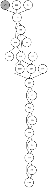
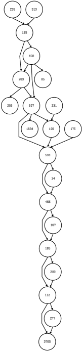
Figure 3: Gene POGZ. The isoform graph (on the left) and the splicing graph (on the right) predicted in the third experiment. The difference between the two graphs consists of the gray vertex that is missing in the splicing graph.

The final part of our analysis is a comparison with Trinity [11] – the most advanced available tool for full-length transcript reconstruction from RNA-Seqs without a reference genome, to determine how much it is stable. We have run Trinity on the two full coverage datasets, corresponding to the first and third experiments. Since Trinity computes transcripts and not the splicing graph, we use the variation of number of predicted full-lengths transcripts as a proxy for the (in)stability of the method. We observed that, for the two datasets, Trinity has predicted $2689$ and $1694$ full-length transcripts (on the genes from which the simulated read are generated, there are $1020$ annotated transcripts). The variation is significant and hints at a desired property of our algorithm that is not shared with other state-of-the-art tools.

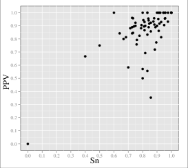
Figure 4: Second experiment: Sn and PPV values at vertex level. Each point represents a gene.

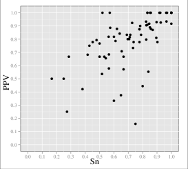
Figure 5: Second experiment: Sn and PPV values at arc level. Each point represents a gene.

References

- [1] M. L. Metzker, “Sequencing technologies - the next generation.” Nature reviews. Genetics, vol. 11, no. 1, pp. 31–46, 2010.
- [2] C. Trapnell, B. A. Williams, G. Pertea, A. Mortazavi, et al. “Transcript assembly and quantification by RNA-Seq reveals unannotated transcripts and isoform switching during cell differentiation,” Nature Biotechnology, vol. 28, no. 5, pp. 516–520, 2010.
- [3] M. Nicolae, S. Mangul, I. I. Mandoiu, and A. Zelikovsky, “Estimation of alternative splicing isoform frequencies from RNA-Seq data.” Algorithms for molecular biology : AMB, vol. 6, no. 1, p. 9, 2011.
- [4] J. Feng, W. Li, and T. Jiang, “Inference of isoforms from short sequence reads,” Journal of Computational Biology, vol. 18, no. 3, pp. 305–321, 2011.
- [5] S. Heber, M. A. Alekseyev, S.-H. Sze, H. Tang, and P. A. Pevzner, “Splicing graphs and EST assembly problem,” in Proc. 10th Int. Conf. on Intelligent Systems for Mol. Biology (ISMB), vol. 18, pp. 181–188, 2002.
- [6] V. Lacroix, M. Sammeth, R. Guigó, and A. Bergeron, “Exact transcriptome reconstruction from short sequence reads,” in Proc. 8th Int. Workshop on Algorithms in Bioinformatics (WABI), ser. LNCS, vol. 5251. Springer, 2008, pp. 50–63.
- [7] M. Garber, M. Grabherr, M. Guttman, and C. Trapnell, “Computational methods for transcriptome annotation and quantification using RNA-Seq,” Nature Methods, vol. 8, no. 6, pp. 469–77, 2011.
- [8] M. Guttman, G. Manuel, J. Levin, J. Donaghey, et al. “From Ab initio reconstruction of cell type–specific transcriptomes in mouse reveals the conserved multi-exonic structure of lincRNAs,” Nature Biotechnology, vol. 28, pp. 503–510, 2010.
- [9] G. Robertson, J. Schein, R. Chiu, et al. “De novo assembly and analysis of RNA-seq data” Nature Methods, vol. 7, no. 5, pp. 909–912, 2010.
- [10] D. Zerbino and E. Birney, “Velvet: Algorithms for de novo short read assembly using de Bruijn graphs,” Genome Research, vol. 18, pp. 821–829, 2008.
- [11] M. Grabherr, B. Haas, M. Yassour, J. Levin, et al. “Full-length transcriptome assembly from RNA-Seq data without a reference genome,” Nature Biotechnology, vol. 29, no. 7, pp. 644–652, 2011.
- [12] R. Guigó, P. Flicek, J. Abril, A. Reymond, et al. “EGASP: the human ENCODE Genome Annotation Assessment Project.” Genome biology, vol. 7, no. Suppl 1, pp. S2.1–31, 2006.
- [13] S. Altschul, W. Gish, W. Miller, E. Myers, and J. Lipman, “Basic local alignment search tool,” J. of Mol. Biology, vol. 215, pp. 403–410, 1990.