Transient and finite size effects in transport properties of a quantum wire

Abstract

We study the time-dependent backscattered current produced in a quantum wire when a local barrier is suddenly switched on. Previous investigations are improved by taking into account the finite length of the device. We establish two different regimes in terms of the relationship between the energy scales associated to the voltage and the length of the system. We show how previous results, valid for wires of infinite length, are modified by the finite size of the system. In particular our study reveals a rich pattern of temporal steps within which the current suffers an initial relaxation followed by temporary revivals. By employing both analytical and numerical methods we describe peculiar features of this structure. From this analysis one concludes that our results render a recently proposed approach to the determination of the Luttinger parameter $K$, more realistic.

I Introduction

Recently there has been much interest in the study of quantum transport in quasi-one-dimensional (1D) materials, such as quantum wires and carbon nanotubes Giamarchi (2004); Di Ventra (2008); Nazarov and Blanter (2009). In 1D systems the effect of electron-electron (e-e) correlations cannot be disregarded, giving rise to a dramatic departure from the Fermi liquid picture of usual condensed matter systems. This new state of matter is called a Luttinger liquid (LL)Voit (1995), and is characterized by correlation functions that decay with distance through exponents that depend on the e-e interaction Bockrath et al. (1999). This peculiar behavior leads to the prediction of striking phenomena such as spin-charge separation and charge fractionalization, both experimentally confirmedAuslaender et al. (2005); Jompol et al. (2009) Steinberg et al. (2008). It is specially interesting to analyze time-dependent aspects of transport Cini (1980); Pastawski (1992); Wingreen et al (1993); Arrachea (2002) in this context. Indeed, the interplay between correlation-induced effects and dynamical phenomena, originated in the out of equilibrium nature of transport, is a highly non trivial problem that deserves much attention. In fact, a detailed knowledge of the LL behavior in the presence of time-dependent perturbations will facilitate the development of devices based on quantum computation, single electron transport and quantum interferometersFujisawa et al (2006); Foa et al (2009). But there is also a more profound motivation to discuss this problem, since it is directly connected to basic issues such as the evolution of the ground state and currents after a quench, according to the influence of different initial conditions Cazalilla (2006); Perfetto et al. (2010b). In a recent workSalvay et al. (2010) we have analyzed the response of a LL (formed by electrons in a quantum wire) to a sudden switch of an interaction of the system with an external field (a local barrier created by applying a voltage to a narrow metal gate electrode in a single-walled carbon nanotube Biercuk et al. (2004); Biercuk et al. (2005a, b)). When such a barrier, that can be considered as a backscattering impurity, is turned on at a finite time $t_{0}$, a backscattered current $I_{bs}$ is produced. In Ref. Salvay et al., 2010 a quantitative relation between the time evolution of $I_{bs}$ and the constant $K$, related to e-e correlations, was obtained. Thus, it was shown that $K$ could be determined by measuring time intervals within the reach of recently developed pump-probe techniques with femtosecond-attosecond time resolutions Gouielmakis et al. (2007). This result was obtained under the assumption that the length of the wire was infinite. It is then very important, in order to make the predictions more realistic, to understand the role that the finite size of the sample will play in the time evolution of the electrical current. This is the main purpose of this article. It is worth mentioning that the effects of finite length of a quantum wire on its transport properties were previously investigated in Refs. Ponomarenko and Nagaosa, 1997, Dolcini et al., 2003, Dolcini et al., 2005 and Cheng and Zhou, 2006, but for the case of a static impurity. Besides its direct interest in the area of one-dimensional strongly correlated systems, our work reveals some general features of time-dependent transport in confined geometries that could contribute to a deeper understanding of the behavior of other materials, such as graphene nanoribbons under the sudden switch-on of a constant electric field Lewkowicz and Rosenstein (2009) or a constant bias voltage Perfetto et al. (2010a). Another interesting problem, closely connected with our findings, is the role of interacting leads in transport through a quantum point-contact. Concerning this issue it has been recently shown that the switching process has a large impact on the relaxation and the steady-state behavior of the current Perfetto et al. (2010b). However, for the sake of clarity let us stress that, in contrast to the situation discussed in Ref.Perfetto et al., 2010b, where the interaction between the wire and the contacts that leads to the bias voltage V is also switched on at a given time, here we only consider the switching of the time-dependent impurity, whereas the external voltage is assumed to act at all times. Our study is also of interest in the context of cold atomic gases, where quantum quenches are being intensively investigated Greiner et al. (2002); Cazalilla (2006); Kollath et al. (2007); Cramer et al. (2008); Iucci and Cazalilla (2009); Iucci and Cazalilla (2010); Trotzky et al. (2011).

The paper is organized as follows. In Section II we present the model and define the backscattered current $I_{bs}$. In Section III, in order to facilitate the understanding of our main results, concerned with finite size effects, we recall the results obtained for an infinite wire. Section IV contains the original contributions of this paper. We present a closed expression that gives the time-dependence of the backscattered current as an integral of a function that contains, through an infinite product, the effect of the finite length $L$ of the wire and the position of the impurity. By combining both analytical and numerical methods, we examine the evolution of the current for different wire sizes (Figs. 2-4). Finally, in Section V, we summarize our results and conclusions.

II The model

We consider a clean Luttinger liquid of length $L$ adiabatically coupled to two electrodes at its end points ($x=\pm L/2$) with chemical potentials $\mu_{L}$ and $\mu_{R}$. This gives rise to an applied constant external voltage $V=(\mu_{L}-\mu_{R})/e$, where $e$ is the charge of an electron. We restrict our study to the case in which the electrodes are held at the same temperature. This condition is very important in order to apply standard bosonization techniques Stone (1994); Gogolin et al. (1998). Indeed, as was recently explained in Ref. Gutman et al., 2010, standard bosonization is expected to work well only in special situations corresponding to small deviations from equilibrium. Under this condition the background current flowing in the wire is $I_{0}=e^{2}V/h$ Maslov et al. (1995); Safi et al. (1995). If a point like impurity is switched on in the wire at finite time, a contribution additional to $I_{0}$ due the effect of this impurity appears and the total current now is $I=I_{0}-I_{bs}(t)$. In order to compute $I_{bs}$, after employing the usual bosonization technique Chamon et al. (1995); Makogon et al. (2006), the system is described by the following Lagrangian density:

$$\mathcal{L}=\mathcal{L}_{0}+\mathcal{L}_{\text{imp}}.$$ (1)

The first term describes the dynamics of the conduction electrons and is modeled by a spinless Tomonaga-Luttinger liquid with renormalized Fermi velocity $v$,

$$\mathcal{L}_{0}=\frac{1}{2}\Phi(x,t)\left(v^{2}\frac{\partial^{2}}{\partial x^{2}}-\frac{\partial^{2}}{\partial t^{2}}\right)\Phi(x,t),$$ (2)

where the bosonic field $\Phi$ is related to the charge density $\Phi=e\sqrt{K}\frac{1}{2\pi}\partial_{x}\rho$, $v=v_{F}/K$ when $|x|<L/2$ and $v=v_{F}$ when $|x|>L/2$, where $v_{F}$ is the Fermi velocity and $K$ represents the strength of the electron-electron interactions. For repulsive interactions $K<1$, and for noninteracting electrons $K=1$. The second term contains the impurity contribution producing backscattering of incident waves at the point $x_{0}$,

$$\mathcal{L}_{\text{imp}}=-\frac{g_{b}}{\pi\hbar\Lambda}\delta(x-x_{0})W(t)\\ \times\cos\left[2k_{\text{F}}x/\hbar+2\sqrt{\pi Kv}\Phi(x,t)+eVt/\hbar\right],$$ (3)

where the function $W(t)$ models the way in which the barrier is switched on. In this work we restrict our analysis to the case of a sudden switch that takes place at $t=t_{0}$: $W(t)=\Theta(t-t_{0})$. $\Lambda$ is a short-distance cutoff. We only consider backscattering between electrons and impurities, since at the lowest order in the perturbative expansion in the coupling $g_{b}$ forward scattering does not change the transport properties studied here.

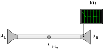
Figure 1: (Color online) The figure shows a quantum wire coupled adiabatically to two reservoirs with different chemical potentials, with a backscattering impurity switched on at time $t=t_{0}$. The current $I(t)$ is measured as a function of time.

The backscattered contribution to the current at any time $t$ is given by

$$I_{bs}(t)=\langle 0|S(-\infty;t)\widehat{I}_{bs}(t)S(t;-\infty)|0\rangle.\,$$ (4)

Here $|0\rangle$ denotes the initial state and $S$ is the scattering matrix, which to the lowest order in the coupling $g_{b}$ is

$$S(t;-\infty)=1-i\int^{\infty}_{-\infty}dx\int^{t}_{-\infty}\mathcal{L}_{\text{imp}}(t^{\prime})dt^{\prime}\,.$$ (5)

$\widehat{I}_{bs}(t)$ is the operator associated to the backscattered current which measures the rate of change of the total number of right movers in the system due to the backscattering impurity Feldman and Gefen (2003); Sharma and Chamon (2003); Agarwal and Sen (2007); Salvay (2009),

$$\widehat{I}_{bs}(t)=\frac{g_{b}e}{\pi\hbar\Lambda}\Theta(t-t_{0})\sin\left[\frac{2k_{F}x_{0}}{\hbar}+2\sqrt{\pi Kv}\widehat{\Phi}(x_{0},t)+\frac{eVt}{\hbar}\right].$$ (6)

To avoid confusion, notice that $\widehat{I}_{bs}(t)$ is, by definition, independent of the position on the wire $x$. Indeed, since it is connected with the time evolution of the total number of right moving particles, it involves an integral of the corresponding density over the $x$-variable. Of course, it does depend on the position of the impurity $x_{0}$, due to the ultralocal impurity Hamiltonian derived from (3). In order to compute $I_{bs}$ one substitutes Eq. (5) into Eq. (4) and finds a series of contributions of the form

$$F(t-t^{\prime})=\langle 0|\exp[2i\sqrt{\pi Kv}\widehat{\Phi}(x_{0},t^{\prime})]\exp[-2i\sqrt{\pi Kv}\widehat{\Phi}(x_{0},t)]|0\rangle.$$ (7)

In order to explicitly evaluate the average appearing in Eq. (7) we employ the Keldysh formalism, a well known technique that renders the study of nonequilibrium systems more accessible Lifshitz and Pitaevskii (1980); Mahan (2007); Das (1997); Kamenev and Levchenko (2009). We use Baker-Haussdorff formula and the fact that the commutator of the $\widehat{\Phi}$-fields is a c-number. This allows to write the v.e.v. of an exponential as the exponential of a v.e.v.. The result is an expression that depends on Keldysh lesser function $iG^{<}(x,t;x,t^{\prime})=\langle 0|\widehat{\Phi}(x,t^{\prime})\,\widehat{\Phi}(x,t)|0\rangle$. This function depends, of course, on the size of the system Mattsson et al. (1997), acquiring a simple form for $L\rightarrow\infty$. In the next section, in order to make the interpretation of the new, finite size effects, more transparent, we will briefly recall the main results obtained in Ref. Salvay et al., 2010 for an infinite wire.

III Results for $L\to\infty$

Restricting our analysis to the zero temperature limit (See Ref. Salvay et al., 2010 for the extension to finite temperatures), (7) reduces to

$$F(t-t^{\prime})=\frac{\Lambda^{2K}\exp[i\pi K\operatorname{sign}[t-t^{\prime}]]}{|v(t-t^{\prime})|^{2K}}\,,$$ (8)

where $\operatorname{sign}$ is the Sign function. First of all, we compute (4) with the impurity switched on at time $-\infty$ :

$$I_{bs}(\infty)=\frac{g_{B}^{2}e\Lambda^{2K-2}}{2\pi\hbar^{2}v^{2K}\Gamma[2K]}\left|\frac{eV}{\hbar}\right|^{2K-1}\operatorname{sign}[V].$$ (9)

This corresponds to the well-known case of a static impurityKane and Fisher (1992), where the backscattered current goes as $V^{2K-1}$. We note that for $K<1/2$, the backscattered current becomes large when $V$ decreases. Hence, the perturbative expansion in powers of $g_{B}$ breaks down when $V\rightarrow 0$. Using a scaling analysis we can estimate that this expansion is valid when $\frac{g_{B}}{\hbar v}(\frac{\Lambda eV}{\hbar v})^{K-1}\ll 1$. We emphasize that expression (9) does not include the case $V=0$, where the current is zero too. All these statements imply that the current must be a nonmonotonic function of $V$. In order to determine this function one has to go beyond the lowest-order perturbative results of this work.

When the impurity is switched on at a finite time $t_{0}$, the current exhibits for finite times a relaxation dynamics to its asymptotic value $I_{bs}(\infty)$. The time-dependent backscattering current dynamics acquires a complicated form, yet it can be written in terms of known analytic functions:

$$I_{bs}(t-t_{0})=\frac{\Theta(t-t_{0})\Gamma[2K][\omega_{0}(t-t_{0})]^{2-2K}}{\Gamma[K]\Gamma[2-K]}\\ \times{}_{1}F_{2}(1-K;3/2,2-K;-[\omega_{0}(t-t_{0})/2]^{2})\,I_{bs}(\infty),$$ (10)

where ${}_{1}F_{2}$ is the generalized hypergeometric function and $\omega_{0}=\frac{e|V|}{\hbar}$ is the Josephson frequency related to the source voltage. This is a damped oscillatory function of $\omega_{0}(t-t_{0})$ with period $2\pi$ and relative maxima in $\omega_{0}(t-t_{0})=(2n+1)\pi$ with $n$ natural. In the long times regime $\omega_{0}(t-t_{0})\gg 1$, this expression can be approximated by its asymptotic form

$$I_{bs}(t-t_{0})\approx\Theta(t-t_{0})\{1\\ -\frac{[\omega_{0}(t-t_{0})]^{-2K}}{\cos[\pi K]\Gamma[1-2K]}\cos[\omega_{0}(t-t_{0})]\}I_{bs}(\infty).$$ (11)

Since the change in the backscattered current due to the sudden switching behaves as $(t-t_{0})^{-2K}$, we conclude that the relaxation of the system is faster for small electron-electron interaction (For the sake of clarity, let us stress that this relaxation characterizes the transition of the backscattering current between two off-equilibrium regimes). We thus find an explicit connection between electron interactions and the switching time of the externally controlled barrier: the stronger the correlations, the longer the persistence of the non adiabatic effect. A determination of the current as function of time with a temporal resolution smaller than $\frac{2\pi}{\omega_{0}}$ is a direct method to obtain the exponent of the temporal decay, and then, the $K$ value of the quantum wire. We emphasize that this proposed method is performed at constant source-drain voltage.

IV Finite size and switching effects

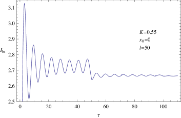
Figure 2: Typical behavior of $I_{bs}$ in units of $I_{bs}(\infty)$ for $\ell\gg 1$ and the impurity located at the center of the wire.

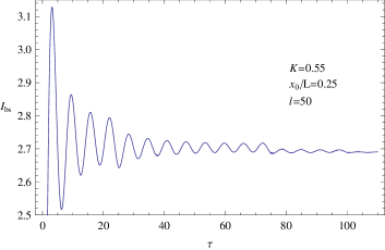
Figure 3: Typical behavior of $I_{bs}$ in units of $I_{bs}(\infty)$ for $\ell\gg 1$ and the impurity located at $x_{0}/L=0.25$.

In this section we present the main results of this work. We will show how the combined effects of a sudden switch-on of an externally controlled barrier and the quantum interference originated by reflections at the ends of the wire (which are now at finite distances from the barrier), modify the time evolution of the backscattered current. The crucial point is that, when the wire has a finite length $L$ the function (7) becomes dependent on $L$ and $x_{0}$. In this case we obtain

$$F(t-t^{\prime})=\prod_{n\text{ even}}\left[\frac{(\delta+i\omega_{B}(t-t^{\prime}))^{2}+n^{2}}{\delta^{2}+n^{2}}\right]^{-K\gamma^{|n|}}\\ \times\prod_{n\text{ odd}}\left[\frac{(\delta+i\omega_{B}(t-t^{\prime}))^{2}+(n-2x_{0}/L)^{2}}{\delta^{2}+(n-2x_{0}/L)^{2}}\right]^{-K\gamma^{|n|}}.$$ (12)

where $\gamma=(1-K)/(1+K)$ is the Andreev-like reflection parameter, $\omega_{B}=v_{F}/KL$ is the ballistic frequency related to the system length and $\delta=\Lambda/L$. In view of this result, from now on we shall write $F(t)\equiv F(\omega_{B}t)$. At this point, replacing (12) in (4), we find the following expression for $I_{bs}$:

$$I_{bs}(t-t_{0})=C\Theta(t-t_{0})\int^{t-t_{0}}_{0}dt^{\prime}\sin(\omega_{0}t^{\prime})\operatorname{Im}F(\omega_{B}t^{\prime}),$$ (13)

where $C=\frac{-eg_{B}^{2}\operatorname{sign}[V]}{\pi^{2}\hbar^{2}\Lambda^{2}}$. This is the generalization, for finite $L$, of the result first obtained in Ref. (Salvay et al., 2010) for an infinitely long wire. As a first test of the validity of this expression we have checked that taking the limit $L\rightarrow\infty$ one recovers the result given in Eq.(10). In contrast to that case, in the present situation the derivation of an approximate expression that could facilitate the physical interpretation is not a trivial task. Despite of this fact, it is possible to obtain an analytical expression for (13) following the lines explained in Ref. (Ponomarenko and Nagaosa, 1997). Let us first define the dimensionless parameter $\ell=\omega_{0}/\omega_{B}$ so that for $\ell\gg(\ll)1$ we have the case of large (small) length. (For example, for applied voltages of order $1mV$ and $1\mu V$, this corresponds to lengths of order $L\gg(\ll)10^{-6}m$ and $L\gg(\ll)10^{-3}m$, respectively). For $\ell\gg 1$ one can get an asymptotic expansion for the current, taking into account that the function $F(\omega_{B}t)$ has an infinite series of cuts in the complex z-plane ($z=\omega_{B}t$), going from $z=i\infty\pm 2n$ to $z=i\delta\pm 2n$ and from $z=i\infty\pm(2n+1)(1+2x_{0}/L)$ to $z=i\delta\pm(2n+1)(1+2x_{0}/L)$, with $n$ integer. The integral can be cast as a sum of contours going around these cuts. The result is a lengthy expression. For the sake of clarity, we will display here the result for the symmetrical case ($x_{0}=0$), which contains the main ingredients needed for a physical interpretation and at the same time acquires a more compact form:

$$I_{bs}(\tau)=-\Theta(\tau)I_{bs}(\infty)\operatorname{Im}\Bigg{\{}2\Gamma[2K]\sin[\pi K]\frac{\tau^{1-2K}e^{-i\tau}}{\pi(1-2K)}\Phi(1,2-2K,i\tau)\\ +\sum_{n=1}^{\infty}\frac{D_{n}\,\ell^{2K(\gamma^{n}-1)}}{\pi(1-2K\gamma^{n})}2\sin(\pi K)\Gamma[2K]\Big{[}(nl+\tau)^{1-2K\gamma^{n}}e^{-i\tau}\Phi(1,2-2K\gamma^{n},i(nl+\tau))\\ -(nl-\tau)^{1-2K\gamma^{n}}e^{+i\tau}\Phi(1,2-2K\gamma^{n},i(nl-\tau))\Big{]}\\ +\sum_{n=1}^{\infty}\frac{D_{n}\,\ell^{2K(\gamma^{n}-1)}}{\pi(1-2K\gamma^{n})}\Theta(\tau-n\ell)2\sin(2\pi K\gamma^{n})\Gamma[2K]e^{i\pi K}e^{-i\tau}(\tau-nl)^{1-2K\gamma^{n}}\Phi(1,2-2K\gamma^{n},i(\tau-nl))\Bigg{\}}$$ (14)

where $\Phi$ is the Kummer confluent hypergeometric function and we have defined $\tau=\omega_{0}(t-t_{0})$ and the numerical coefficient:

$$D_{n}=2^{-2K\gamma^{n}}n^{2K(\gamma^{n}-1)}\prod^{\infty}_{m\neq n,m>0}|\frac{m^{2}}{m^{2}-n^{2}}|^{2K\gamma^{m}}.$$ (15)

Equation (14) turns out to be a valuable tool in order to understand the mechanisms that govern the transient process of $I_{bs}$, even in the general case ($x_{0}=0$).

In Figures 2 and 3 we display the time evolution of $I_{bs}$ as a function of $\omega_{0}t$ (we set $t_{0}=0$) for long wires ($\ell\gg 1$), with the barrier at the center ($x_{0}=0$) and displaced ($x_{0}/L=0.25$). The current evolves through “temporal steps” that take place in $\tau$-regions with ends at $\tau=2n\ell$ and $\tau=(2n+1\pm 2x_{0}/L)\ell$. For $x_{0}=0$ the occurrence of these steps becomes apparent through the functions $\Theta(\tau-n\ell)$ appearing in the analytical expression (14), in which each term represents a new step. One can deduce an expression that describes these steps by retaining only the long times asymptotics in Eq. (14):

$$I_{bs}^{steps}(\tau)=\Theta(\tau)I_{bs}(\infty)\left\{1+2\sum_{n=1}^{\infty}D_{n}\frac{\Gamma(2K)\cos[nl-\pi K(1+\gamma^{n})]}{\Gamma(2K\gamma^{n})\ell^{2K(1-\gamma^{n})}}\Theta(\tau-n\ell)\right\}$$ (16)

In the limit $\tau\to\infty$ Eq. (16) reduces to the static value of the current. In this last case, the current is a damped oscillatory function of $\ell$ with period $2\pi$ and the dominant exponent in the decay is $2K(1-\gamma)$, i.e the current has the form $I_{bs}\approx I_{bs}(\infty)(1+C_{0}\cos[\ell-\pi K(1+\gamma)]\ell^{-2K(1-\gamma)})$, where $C_{0}$ is a coefficient that depends of $K$. When $x_{0}\neq 0$, $I_{bs}$ is a superposition of two damped oscillatory functions of $\ell$ with period $2\pi/(1\pm 2x_{0}/L)$ and the dominant exponent in the decay is $2K(1-\gamma/2)$ (the same for both functions).

In addition to (16), Eq. (14) exhibits an oscillatory behavior in $\tau$ with period equal to $2\pi$ and maxima located at $\tau=(2m+1)\pi$ as in the infinite length case. Those $\tau$-regions are more pronounced and become more visible for $K\ll 1$, i.e. transitory effects originated in the abrupt switching are more important for stronger correlations between electrons. For very long times the current approaches the value corresponding to the case in which one has a static impurity immersed in a wire of length $L$.

Now, we analyze the envelope of the oscillatory function found for the backscattered current, for the case of a long wire ($l\gg 1$). First of all one observes that, in contrast to the case $L\rightarrow\infty$, this envelope is not a monotonic function anymore. Within each $\tau$-window (letting aside, of course, the first abrupt growth at $t=0$) there is an initial decay, followed by a revival of the current that lasts until the beginning of the next step. Again, when the impurity is at the center of the wire (See Fig. 2), the power laws that govern the evolution of $I_{bs}$ can be read from (14). In each of these initial relaxation processes the envelope of the current behaves as $(\tau-n\ell)^{-2K\gamma^{n}}$, for $1+n\ell<\tau\ll(n+1)\ell$, $n$ being a natural number that labels the windows. In particular, at the beginning of the first temporal step that corresponds to $n=0$ (that is, the “short time” region $(\tau\ll\ell)$), the decay is the same as in the case of an infinite wire, found in (11): $\tau^{-2K}$.

For an asymmetrical arrangement in which $x_{0}\neq 0$, the general pattern of the evolution is distorted (See Fig. 3). In particular the heights of the temporal steps (the values of the current envelope in each step) do not decrease monotonically, and their durations are not all equal (they were all equal to $\ell$ when $x_{0}=0$). Moreover, these durations follow an alternated pattern of the form $\Delta\tau_{1}$, $\Delta\tau_{2}$, $\Delta\tau_{1}$, with $\Delta\tau_{1}=(1-2x_{0}/L)\ell$ and $\Delta\tau_{2}=(4x_{0}/L)\ell$ (Note that $2\Delta\tau_{1}+\Delta\tau_{2}=2\ell$). The decay laws that we found for these $\tau$-windows are:

$$(\tau-2p\ell)^{-2K\gamma^{2p}}$$

for $1+2p\ell<\tau\ll 2p\ell+\ell(1-2x_{0}/L)$;

$$(\tau-2p\ell-\ell(1-2x_{0}/L))^{-K\gamma^{2p+1}}$$

for $1+2p\ell+\ell(1-2x_{0}/L)<\tau\ll 2p\ell+\ell(1+2x_{0}/L)$ and

$$(\tau-2p\ell-\ell(1+2x_{0}/L))^{-K\gamma^{2p+1}}$$

for $1+2p\ell+\ell(1+2x_{0}/L)<\tau\ll(2p+2)\ell$. Here the natural number $p$ does not label windows. The value $p=0$ gives the behavior corresponding to the first three $\tau$-windows that appear in the interval $0<\tau<2\ell$. This basic pattern is repeated along the subsequent intervals of duration $2\ell$, the corresponding exponents are given by the following values of $p$.

A word of caution is in order here regarding the limit $x_{0}\rightarrow 0$. Notice that when considering this limit in the expressions above one does not recover the exponents for an impurity placed at the center of the wire. This is so because the correlation function corresponding to the general case ($x_{0}\neq 0$) has pairs of different singularities that merge when $x_{0}=0$. A similar situation is discussed in the study of finite length effects for an static impurity presented in Ref.Dolcini et al., 2005.

The relationship between the relaxation process and the strength of Coulomb electron correlations revealed in our analysis provides an alternative way to determine the Luttinger parameter $K$ through time measurements. Since the total current has the form $I_{0}-I_{bs}(t)$, a determination of the current as a function of time (keeping the source-drain voltage constant) with a temporal resolution smaller than $2\pi\hbar/eV$, enables to obtain the exponent of the temporal decay, and then the $K$ value of the quantum wire. Interestingly, having taken into account the finite size of the system, our results suggest another possible experimental application. Indeed, the experimental determination of the duration of the $\tau$-windows described above allows to obtain the value of the ratio of Josephson to ballistic frequencies $\ell=\frac{eVL}{\hbar}\frac{K}{v_{F}}$. Thus, if $V$, $L$ and the Fermi velocity $v_{F}$ are known (the last one can be obtained by photoemission spectroscopy), this simple technique gives another way of finding the Luttinger parameter.

Finally, for completeness, we explore transport properties in short wires ($\ell<1$). In this case the asymptotic expansion described above is not valid and then we are led to analyze Eq. (13) numerically. In Figure 4 we show the behavior of $I_{bs}$ for short wires . In this case the structure of “temporal steps” disappears and finite-time switching effects are relevant for $\omega_{0}t\leq 1$. In this regime one observes a monotonous growth of the backscattered current, with discontinuities in the time-derivative that take place at $\omega_{0}t=2n\ell$ and $\omega_{0}t=(2n+1\pm 2x_{0}/L)\ell$. For $\omega_{0}t>1$ the current also tends to the static-impurity value $I_{bs}(\infty)$, as expected. Thus, in practice, for short wires, the oscillation of the current as function of $\omega_{0}t$ ceases to be appreciable. This is due to the fact that, for fixed $K$ and $V$, the Josephson current $\omega_{0}$ becomes negligible when compared with the ballistic frequency $\omega_{B}$. In contrast to what happens for long wires, where an ultrafast current growth is followed by an oscillatory decay pattern, here $I_{bs}$ undergoes a rapid increase towards the steady-state current, which goes as $\ell^{2-2K}$ and has a monotonic decrease with $|x_{0}/L|$. In this sense one could say that, in a sufficiently short wire, instead of a relaxation process (after the initial jump), a monotonic enhancement, saturating at the steady-state current, is predicted.

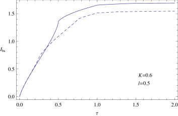
Figure 4: Typical behavior of $I_{bs}$ in units of $I_{bs}(\infty)$ for $\ell<1$ and the impurity located at $x_{0}=0$ (solid line) and $x_{0}/L=0.25$ (dashed line).

V Conclusions

To summarize, we have analyzed the characteristics of time-dependent transport in a Tomonaga-Luttinger liquid subjected to a constant bias voltage, when a weak barrier is suddenly switched on. The novel features of our investigation come from the consideration of a wire with a finite length $L$. We focused our attention on the backscattered current $I_{bs}$ which is originated by the abrupt appearance of the barrier. We showed that, in comparison with the case $L\rightarrow\infty$, for which the current relaxes to the steady-state value with an envelope that obeys the simple law $t^{-2K}$, finite size effects lead to a much more complex and rich evolution. In order to grasp the main features of this dynamics, we have identified different regimes in terms of the Josephson frequency $\omega_{0}=\frac{e|V|}{\hbar}$ and the ballistic frequency $\omega_{B}=\frac{v_{F}K}{L}$. In particular, when the applied bias ($V$) and the electron-electron correlations ($K$) are held fixed, the ratio $\ell=\omega_{0}/\omega_{B}$ provides a natural parameter to characterize “long” ($\ell\gg 1$) and “short” ($\ell\ll 1$) wires. In this context it becomes natural to compare the results obtained for $\ell\gg 1$ with the previously known behavior found in infinite systems. We found that for long sizes the evolution of $I_{bs}$ presents a new structure of temporal steps, each of which with a different decay law with the generic form $(t-\nu)^{-\mu K\gamma^{m-1}}$, where $\nu$ depends on $m$, $\omega_{B}$ and $x_{0}$, and $\gamma=(1-K)/(1+K)$ is an Andreev-like reflection parameter. The constant $\mu$ is simply 1 or 2, depending on the $\tau$-step one is looking at. Since $K<1$ and $m$ is a natural number that labels each time window, being $m$ bigger for longer times, the older the window the slower the relaxation. These results display the way in which the combined effects of electronic correlations and quantum interference, originated by reflected waves at the interfaces with the electrodes, affect the transient process.

Concerning short wires, the whole structure of temporal steps disappears and the evolution becomes simpler, showing a monotonic growth of $I_{bs}$ towards its steady-state value.

From the point of view of the potential applications of our study it is specially interesting the case of long wires, for which we were able to derive approximate asymptotic expressions from which one determines the durations of the temporal steps and the power laws obeyed by the envelope of the current in the time intervals where a relaxation takes place. If one measures the decay of the current along these intervals, the value of $K$ can be obtained from the exponents $\mu K((1-K)/(1+K))^{m-1}$, where the values of both $\mu$ and $m$ are univocally given by the $\tau$-window for which the measurement is performed. A second method, probably easier to implement, is also indicated by our findings. Indeed, as explained in the text, just by measuring the endpoints of the $\tau$-windows, taking into account that $L$ and $x_{0}$ are assumed to be known (remember that in the context of our investigation the impurity is assumed to be due to an external gate), one can determine the value of $\ell=\frac{eVL}{\hbar}\frac{K}{v_{F}}$. Since the bias voltage $V$ is also externally controlled and held fixed, this simple technique gives a direct way of finding the ratio $\frac{K}{v_{F}}$. Of course, if one of these two parameters are known by means of another reliable method, the remaining one is directly obtained from our recipe.