Symplectic bifurcation theory for integrable systems

Abstract

This paper develops a symplectic bifurcation theory for integrable systems in dimension four. We prove that if an integrable system has no hyperbolic singularities and its bifurcation diagram has no vertical tangencies, then the fibers of the induced singular Lagrangian fibration are connected. The image of this singular Lagrangian fibration is, up to smooth deformations, a planar region bounded by the graphs of two continuous functions. The bifurcation diagram consists of the boundary points in this image plus a countable collection of rank zero singularities, which are contained in the interior of the image. Because it recently has become clear to the mathematics and mathematical physics communities that the bifurcation diagram of an integrable system provides the best framework to study symplectic invariants, this paper provides a setting for studying quantization questions, and spectral theory of quantum integrable systems.

1 Introduction and Main Theorems

A major obstacle to a symplectic theory of finite dimensional integrable Hamiltonian systems is that differential topological and symplectic problems appear side by side, but smooth and symplectic methods do not always mesh well. Morse-Bott theory represents a success in bringing together in a cohesive way continuous and differential tools, and it has been used effectively to study properties of dynamical systems. But incorporating symplectic information into the context of dynamical systems is far from automatic. However, many concrete examples are known for which computations, and numerical simulations, exhibit a close relationship between the symplectic dynamics of a system, and the differential topology of its bifurcation set.

In the 1980s and 1990s, the Fomenko school developed a Morse theory for regular energy surfaces of integrable systems. Moreover, theoretical successes (in any dimension) for compact periodic systems in the 1970s and 1980s by Atiyah, Guillemin, Kostant, Sternberg and others, gave hope that one can find a mathematical theory for bifurcations of integrable systems in the symplectic setting.

This paper develops a symplectic bifurcation theory for integrable systems in dimension four – compact or not. Because it recently has become clear that the bifurcation diagram of an integrable system is the natural setting to study symplectic invariants (see for instance [38, 39]), this paper provides a setting for the study of quantum integrable systems. Semiclassical quantization is a strong motivation for developing a systematic bifurcation theory of integrable systems; the study of bifurcation diagrams is fundamental for the understanding of quantum spectra [14, 32, 52]. Moreover, the results of this paper may have applications to mirror symmetry and symplectic topology because an integrable system without hyperbolic singularities gives rise to a toric fibration with singularities. The base space is endowed with a singular integral affine structure. These singular affine structures are studied in symplectic topology, mirror symmetry, and algebraic geometry; for instance, they play a central role in the work of Kontsevich and Soibelman [30]. We refer to Section 6 for further analysis of these applications, as well as a natural connection to the study of solution sets in real algebraic geometry.

The development of the theory requires the introduction of methods to construct Morse-Bott functions which, from the point of view of symplectic geometry, behave well near the singularities of integrable systems. These methods use Eliasson’s theorems on linearization of non-degenerate singularities of integrable systems, and the symplectic topology of integrable systems, to which many have contributed.

The first part of this paper is concerned with the connectivity of joint level sets of vector-valued maps on manifolds, when these are defined by the components of an integrable system. The most striking previous result in this direction is Atiyah’s 1982 theorem which guarantees the connectivity of the fibers of the momentum map when the integrable system comes from a Hamiltonian torus action. The second part of the paper explains how the pioneering results proven in the seventies and eighties by Atiyah, Guillemin, Kostant, Kirwan, and Sternberg describing the image of the momentum of a Hamiltonian compact group action also hold in the context of integrable systems on four-dimensional manifolds, when there are no hyperbolic singularities. The conclusions of the theorems in this paper are essentially optimal. Moreover, there is only one transversality assumption on the integrable system: that there should be no vertical tangencies on the bifurcation set, up to diffeomorphism. If this condition is violated then there are examples which show that one cannot hope for any fiber connectivity.

The work of Atiyah, Guillemin, Kostant, Kirwan, and Sternberg exhibited connections between symplectic geometry, combinatorics, representation theory, and algebraic geometry. Their work guarantees the convexity of the image of the momentum map (intersected with the positive Weyl chamber if the compact group is non-commutative). Although this property no longer holds for general integrable systems, an explicit description of the image of the singular Lagrangian fibration given by an integrable system with two degrees of freedom can be given. The understanding of this image, which corresponds to the bifurcation diagram of the dynamics in the physics literature, is essential for the description of the system, as it has proven to be the best framework to define new symplectic invariants of integrable systems, and hence to quantize; see the recent work on semitoric integrable systems [38, 39, 40, 41].

Fiber connectivity for integrable systems

The most striking known result for fiber connectivity of vector-valued functions is Atiyah’s famous connectivity theorem [3] proved in the early eighties.

Connectivity Theorem (Atiyah).

Suppose that $(M,\,\omega)$ is a compact, connected, symplectic, $2m$-dimensional manifold. For smooth functions $f_{1},\,\ldots,\,f_{n}\colon M\to\mathbb{R}$, let $\varphi_{i}^{t_{i}}$ be the flow of the Hamiltonian vector field $\mathcal{H}_{f_{i}}$, where $\mathcal{H}_{f_{i}}$ is defined by the equation $\omega(\mathcal{H}_{f_{i}},\,\cdot)=\mathrm{d}f_{i}$. We denote by ${\mathbb{T}}^{n}$ the $n$-dimensional torus ${\mathbb{R}}^{n}/{\mathbb{Z}}^{n}$. Suppose that $M\ni p\mapsto(\varphi_{1}^{t_{1}}\circ\ldots\circ\varphi_{n}^{t_{n}})(p)\in M$, where $(t_{1},\ldots,t_{n})\in\mathbb{R}^{n}$, defines a ${\mathbb{T}}^{n}$-action on $M$. Then the fibers of the map $F:=(f_{1},\,\ldots,\,f_{n})\colon M\to\mathbb{R}^{n}$ are connected.

This theorem has been generalized by a number of authors to general compact Lie groups actions and more general symplectic manifolds. Indeed, a Hamiltonian $m$-torus action on a $2m$-manifold may be viewed as a very particular integrable system. A long standing question in the integrable systems community has been to what extent Atiyah’s result holds for integrable systems, where checking fiber connectivity by hand is extremely difficult (even for easily describable examples). This paper answers this question in the positive in dimension four: if an integrable system has no hyperbolic singularities and its bifurcation diagram has no vertical tangencies, then the fibers of the integrable system are connected.

To state this result precisely, recall that a map $F=(f_{1},\ldots,f_{n})\colon(M,\,\omega)\to\mathbb{R}^{n}$ is a integrable Hamiltonian system if $\mathcal{H}_{f_{1}},\,\ldots,\mathcal{H}_{f_{n}}$ are point-wise almost everywhere linearly independent and for all indices $i,\,j$, the function $f_{i}$ is invariant along the flow of the Hamiltonian vector field $\mathcal{H}_{f_{j}}$. (Recall: $\mathcal{H}_{f_{i}}$ is the vector field defined by $\omega(\mathcal{H}_{f_{i}},\,\cdot)=\mathrm{d}f_{i}$).

In general, fiber connectivity is no longer true for integrable systems, due to the existence of singularities. For instance, consider the manifold is $M=S^{2}\times S^{1}\times S^{1}$. Choose the following coordinates on $S^{2}$: $h\in[1,\,2]$ and $a\in S^{1}=\mathbb{R}/2\pi\mathbb{Z}$. Choose coordinates $b,c\in\mathbb{R}/2\pi\mathbb{Z}$ on $S^{1}\times S^{1}$ and let $\mathrm{d}h\wedge\mathrm{d}a+n\mathrm{d}b\wedge\mathrm{d}c$ be the symplectic form on $M$, where $n$ is a positive integer. The map $F(h,\,a,\,b,\,c)=(h\cos(nb),\,h\sin(nb))$, defines an integrable system. The fiber over any regular value of $F$ is $n$ copies of $S^{1}\times S^{1}$. The image $F(M)$ is an annulus (see Figure 1).

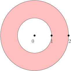
Figure 1: Image $F(M)$ of integrable system with disconnected fibers, on the compact manifold $S^{2}\times S^{1}\times S^{1}$. This integrable system has only singularities of elliptic and transversally elliptic type, so it is remarkable how while being quite close to be a toric system, fiber connectivity is lost.

An annulus has the property that it has vertical tangencies, and it cannot be deformed into a domain without such tangencies. Remarkably, if such tangencies do not exist in some deformation of $F(M)$, fiber connectivity still holds. This is for instance the case for Hamiltonian torus actions. Next we state this precisely.

In this paper, manifolds are assumed to be ${\rm C}^{\infty}$ and second countable. Let us recall here some standard definitions. A map $f\colon X\to Y$ between topological spaces is proper if the preimage of every compact set is compact. Let $X$, $Y$ be smooth manifolds, and let $A\subset X$. A map $f:A\to Y$ is said to be smooth if at any point in $A$ there is an open neighborhood on which $f$ can be smoothly extended. The map $f$ is called a diffeomorphism onto its image when $f$ is injective, smooth, and its inverse $f^{-1}:f(X)\to X$ is smooth. If $X$ and $Y$ are smooth manifolds, the bifurcation set $\Sigma_{f}$ of a smooth map $f:X\rightarrow Y$ consists of the points of $X$ where $f$ is not locally trivial (see Definition 3). It is known that the set of critical values of $f$ is included in the bifurcation set and that if $f$ is proper this inclusion is an equality (see [1, Proposition 4.5.1] and the comments following it).

Second, recall that an integrable system $F\colon M\to\mathbb{R}^{2}$ is called non-degenerate if its singularities are non-degenerate (see Definition 2). If $F$ is proper and non-degenerate, then $\Sigma_{F}$ is the image of a piecewise smooth immersion of a 1-dimensional manifold (Proposition 4.3). We say that a vector in $\mathbb{R}^{2}$ is tangent to $\Sigma_{F}$ whenever it is directed along a left limit or a right limit of the differential of the immersion. We say that the curve $\gamma$ has a vertical tangency at a point $c$ if there is a vertical tangent vector at $c$. Our first main result is the following.

Theorem 1 (Connectivity for Integrable Systems – Compact Case).

Suppose that $(M,\omega)$ is a compact connected symplectic four-manifold. Let $F\colon M\to\mathbb{R}^{2}$ be a non-degenerate integrable system without hyperbolic singularities. Denote by $\Sigma_{F}$ the bifurcation set of $F$. Assume that there exists a diffeomorphism $g\colon F(M)\to\mathbb{R}^{2}$ onto its image such that $g(\Sigma_{F})$ does not have vertical tangencies (see Figure 2). Then $F$ has connected fibers.

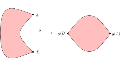
Figure 2: Suppose that the bifurcation set $\Sigma_{F}$ of $F$ consists precisely of the boundary points in the left figure (which depicts $F(M)$). The diffeomorphism $g$ transforms $F(M)$ to the region on the right hand side of the figure, in order to remove the original vertical tangencies on $\Sigma_{F}$.

Remark 1.1   If $F\colon M\to\mathbb{R}^{2}$ in Theorem 2 is the momentum map of a Hamiltonian $2$-torus action then $\Sigma_{F}=\partial(F(M))$. This is no longer true for general integrable systems; the simplest example of this is the spherical pendulum, which has a point in the bifurcation set in the interior of $F(M)$. $\oslash$

We denote by $C_{\alpha,\beta}$ the cone in Figure 3, i.e., the intersection of the half-planes defined by $y\geqslant(\tan\alpha)\,x$ and $y\leqslant(\tan\beta)\,x$ on the plane $\mathbb{R}^{2}$. This cone will be called proper, if $\alpha>0,\,\beta>0$, $\alpha+\beta<\pi$. Theorem 2 can be extended to non-compact manifolds as follows.

Theorem 2 (Connectivity for Integrable Systems – Non-compact Case).

Suppose that $(M,\omega)$ is a connected symplectic four-manifold. Let $F\colon M\to\mathbb{R}^{2}$ be a non-degenerate integrable system without hyperbolic singularities such that $F$ is a proper map. Denote by $\Sigma_{F}$ the bifurcation set of $F$. Assume that there exists a diffeomorphism $g\colon F(M)\to\mathbb{R}^{2}$ onto its image such that:

1. the image $g(F(M))$ is included in a proper convex cone $C_{\alpha,\,\beta}$ (see Figure 3);

2. the image $g(\Sigma_{F})$ does not have vertical tangencies (see Figure 2).

Then $F$ has connected fibers.

Note that Theorem 2 clearly implies Theorem 1.

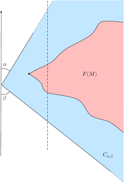
Figure 3: The image $F(M)$ lies in the convex cone $C_{\alpha,\beta}$ and has no vertical tangencies. See condition 1 in theorem 2.

Remark 1.2   The assumption in Theorem 2 is optimal in the following sense: if there exist vertical tangencies then the system can have disconnected fibers (Examples 8, 10); see Theorem 3. Other than these exceptions we do not know of an integrable system with disconnected fibers and which does not violate our assumptions. $\oslash$

Further in this article, we introduce a weaker transversality condition that allows us to deal with some cases of vertical tangencies. Using this condition and Theorem 2, we will prove the following.

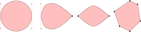
Figure 4: A disk, a disk with a conic point, a disk with two conic points, or a compact convex polygon.

Theorem 3.

Suppose that $(M,\omega)$ is a compact connected symplectic four-manifold. Let $F\colon M\to\mathbb{R}^{2}$ be a non- degenerate integrable system without hyperbolic singularities. Assume that

1. the interior of $F(M)$ contains a finite number of critical values;

2. there exists a diffeomorphism $g$ such that $g(F(M))$ is either a disk, a disk with a conic point, a disk with two conic points, or a compact convex polygon (see Figure 4).

Then the fibers of $F$ are connected.

Here a neighborhood of a conic point is by definition locally diffeomorphic to some proper cone $C_{\alpha,\beta}$.

Structure of the image of an integrable system

Atiyah proved his connectivity theorem [3] simultaneously with the so called convexity theorem of Atiyah, Guillemin, and Sternberg [3, 28]; it is one of the main results in symplectic geometry. Their convexity theorem describes the image of the momentum map of a Hamiltonian torus action. Altogether, this result generated much subsequent research, in particular it led Kirwan to prove a remarkable non-commutative version [29].

Convexity Theorem (Atiyah and Guillemin-Sternberg).

Suppose that $(M,\,\omega)$ is a compact, connected, symplectic, $2m$-dimensional manifold. For smooth functions $f_{1},\,\ldots,\,f_{n}\colon M\to\mathbb{R}$, let $\varphi_{i}^{t_{i}}$ be the flow of the Hamiltonian vector field $\mathcal{H}_{f_{i}}$, where $\mathcal{H}_{f_{i}}$ is defined by the equation $\omega(\mathcal{H}_{f_{i}},\,\cdot)=\mathrm{d}f_{i}$. We denote by ${\mathbb{T}}^{n}$ the $n$-dimensional torus ${\mathbb{R}}^{n}/{\mathbb{Z}}^{n}$. Suppose that $M\ni p\mapsto(\varphi_{1}^{t_{1}}\circ\ldots\circ\varphi_{n}^{t_{n}})(p)\in M$, where $(t_{1},\ldots,t_{n})\in\mathbb{R}^{n}$, defines a ${\mathbb{T}}^{n}$-action on $M$. Then the image of $F:=(f_{1},\,\ldots,\,f_{n})\colon M\to\mathbb{R}^{n}$ is a convex polytope.

Remark 1.3   An important paper prior to the work of Atiyah, Guillemin, Kirwan, and Sternberg dealing with convexity properties in particular instances is Kostant’s [31], who also refers to preliminary questions of Schur, Horn and Weyl. These convexity results were used by Delzant [16] in his classification of symplectic toric manifolds. All together, these papers revolutionized symplectic geometry and its connections to representation theory, combinatorics, and complex algebraic geometry. For a detailed analysis of symplectic toric manifolds in the context of complex algebraic geometry, see Duistermaat-Pelayo [17]. $\oslash$

In this paper we prove the natural version of the Atiyah-Guillemin-Sternberg convexity theorem in the context of integrable systems. Before stating it we recall that the epigraph $\!\!\mathop{\rm~{}epi}\nolimits(f)\subseteq\mathbb{R}^{n+1}$ of a map $f\colon A\subseteq\mathbb{R}^{n}\to\mathbb{R}\cup\{\pm\infty\}$ consists of the points lying on or above its graph, i.e., the set $\!\!\mathop{\rm~{}epi}\nolimits(f):=\{(x,\,y)\in A\times\mathbb{R}\,|\,y\geqslant f(x)\}$. Similarly, the hypograph $\!\!\mathop{\rm~{}hyp}\nolimits(f)\subseteq\mathbb{R}^{n+1}$ of a map $f\colon A\subseteq\mathbb{R}^{n}\to\mathbb{R}\cup\{\pm\infty\}$ consists of the points lying on or below its graph, i.e., the set $\!\!\mathop{\rm~{}hyp}\nolimits(f):=\{(x,\,y)\in A\times\mathbb{R}\,|\,y\leqslant f(x)\}$.

Theorem 4 (Image of Lagrangian fibration of integrable system – Compact Case).

Suppose that $(M,\omega)$ is a compact connected symplectic four-manifold. Let $F\colon M\to\mathbb{R}^{2}$ be a non-degenerate integrable system without hyperbolic singularities. Denote by $\Sigma_{F}$ the bifurcation set of $F$. Assume that there exists a diffeomorphism $g\colon F(M)\to\mathbb{R}^{2}$ onto its image such that $g(\Sigma_{F})$ does not have vertical tangencies (see Figure 2). Then:

• the image $F(M)$ is contractible and the bifurcation set can be described as $\Sigma_{F}=\partial(F(M))\sqcup\mathcal{F},$ where $\mathcal{F}$ is a finite set of rank $0$ singularities which is contained in the interior of $F(M)$;

• let $(J,\,H):=g\circ F$ and let $J(M)=[a,\,b]$. Then the functions $H^{+},\,H^{-}\colon[a,\,b]\to{\mathbb{R}}$ defined by $H^{+}(x):=\max_{J^{-1}(x)}H$ and $H^{-}(x):=\min_{J^{-1}(x)}H$ are continuous and $F(M)$ can be described as $F(M)=g^{-1}(\!\!\mathop{\rm~{}epi}\nolimits(H^{-})\cap\!\!\mathop{\rm~{}hyp}\nolimits(H^{+}))$.

Figure 5 shows a possible image $F(M)$, as described in Theorem 4. In the case on non-compact manifolds we have the following result.

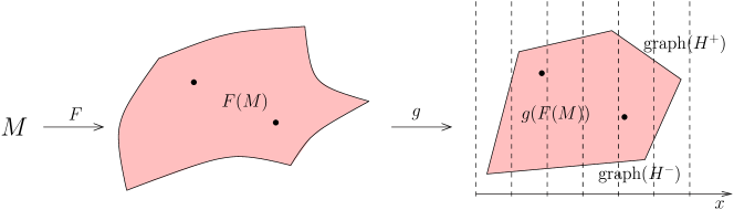
Figure 5: Description of the image of an integrable system. The image is first transformed to remove vertical tangencies, and then it can be described as a region bounded by two graphs.

Theorem 5 (Image of Lagrangian fibration of integrable system – Non-compact case).

Suppose that $(M,\omega)$ is a connected symplectic four-manifold. Let $F\colon M\to\mathbb{R}^{2}$ be a non-degenerate integrable system without hyperbolic singularities such that $F$ is a proper map. Denote by $\Sigma_{F}$ the bifurcation set of $F$. Assume that there exists a diffeomorphism $g\colon F(M)\to\mathbb{R}^{2}$ onto its image such that:

1. the image $g(F(M))$ is included in a proper convex cone $C_{\alpha,\,\beta}$ (see Figure 3);

2. the image $g(\Sigma_{F})$ does not have vertical tangencies (see Figure 2).

Equip $\overline{\mathbb{R}}:=\mathbb{R}\cup\{\pm\infty\}$ with the standard topology. Then:

• the image $F(M)$ is contractible and the bifurcation set can be described as $\Sigma_{F}=\partial(F(M))\sqcup\mathcal{F},$ where $\mathcal{F}$ is a countable set of rank zero singularities which is contained in the interior of $F(M)$;

• let $(J,\,H):=g\circ F$. Then the functions $H^{+},\,H^{-}\colon J(M)\to{\mathbb{R}}$ defined on the interval $J(M)$ by $H^{+}(x):=\max_{J^{-1}(x)}H$ and $H^{-}(x):=\min_{J^{-1}(x)}H$ are continuous and $F(M)$ can be described as $F(M)=g^{-1}(\!\!\mathop{\rm~{}epi}\nolimits(H^{-})\cap\!\!\mathop{\rm~{}hyp}\nolimits(H^{+}))$.

Note that Theorem 5 clearly implies Theorem 4. The rest of this paper is devoted to proving Theorem 2, Theorem 3 and Theorem 5.

Acknowledgements. We thank Denis Auroux, Thomas Baird, and Helmut Hofer for enlightening discussions. The authors are grateful to Helmut Hofer for his essential support that made it possible for TSR and VNS to visit AP at the Institute for Advanced Study during the Winter and Summer of 2011, where a part of this paper was written. Additional financial support for these visits was provided by Washington University in St Louis and by NSF. The authors also thank MSRI, the Mathematisches Forschungsinstitut Oberwolfach, Washington University in St Louis, and the Université de Rennes I for their hospitality at different stages during the preparation of this paper in 2009, 2010, and 2011.

AP was partly supported by an NSF Postdoctoral Fellowship, NSF Grants DMS-0965738 and DMS-0635607, an NSF CAREER Award, a Leibniz Fellowship, Spanish Ministry of Science Grant MTM 2010-21186-C02-01, and by the CSIC (Spanish National Research Council).

TSR. was partly supported by a MSRI membership and Swiss NSF grant 200020-132410.

VNS was partly supported by the NONAa grant from the French ANR and the Institut Universitaire de France.

The paper combines a number of results to arrive at the proofs of these theorems. The following diagram describes the structure of the paper.

2 Basic properties of almost-toric systems

In this section we prove some basic results that we need in of Section 3 and Section 4. Let $(M,\omega)$ be a connected symplectic 4-manifold.

Toric type maps

A smooth map $F\colon M\to\mathbb{R}^{2}$ is toric if there exists an effective, integrable Hamiltonian ${\mathbb{T}}^{2}$-action on $M$ whose momentum map is $F$. It was proven in [33] that if $F$ is a proper momentum map for a Hamiltonian ${\mathbb{T}}^{2}$-action, then the fibers of $F$ are connected and the image of $F$ is a rational convex polygon.

Almost-toric systems

We shall be interested in maps $F:M\rightarrow\mathbb{R}^{2}$ that are not toric yet retain enough useful topological properties. In the analysis carried out in the paper we shall need the concept of non-degeneracy in the sense of Williamson of a smooth map from a 4-dimensional phase space to the plane.

Definition 2.1   Suppose that $(M,\omega)$ is a connected symplectic four-manifold. Let $F=(f_{1},f_{2})$ be an integrable system on $(M,\omega)$, and $m\in M$ a critical point of $F$. If $\mathrm{d}_{m}F=0$, then $m$ is called non-degenerate if the Hessians $\operatorname{Hess}f_{j}(m)$ span a Cartan subalgebra of the symplectic Lie algebra of quadratic forms on the tangent space $({\rm T}_{m}M,\omega_{m})$. If $\operatorname{rank}\left(\mathrm{d}_{m}F\right)=1$ one can assume that $\mathrm{d}_{m}f_{1}\neq 0$. Let $\iota\colon S\to M$ be an embedded local $2$-dimensional symplectic submanifold through $m$ such that ${\rm T}_{m}S\subset\ker(\mathrm{d}_{m}f_{1})$ and ${\rm T}_{m}S$ is transversal to $\mathcal{H}_{f_{1}}$. The critical point $m$ of $F$ is called transversally non-degenerate if $\operatorname{Hess}(\iota^{\ast}f_{2})(m)$ is a non-degenerate symmetric bilinear form on ${\rm T}_{m}S$.

Remark 2.2   One can check that Definition 2 does not depend on the choice of $S$. The existence of $S$ is guaranteed by the classical Hamiltonian Flow Box theorem (see e.g., [1, Theorem 5.2.19]; this result is also called the Darboux-Caratheodory theorem [40, Theorem 4.1]). It guarantees that the condition $\mathrm{d}_{m}f_{1}(m)\neq 0$ ensures the existence of a symplectic chart $(x_{1},x_{2},\xi_{1},\xi_{2})$ on $M$ centered at $m$, i.e., $x_{i}(m)=0,\xi_{i}(m)=0$, such that $\mathcal{H}_{f_{1}}=\partial/\partial x_{1}$ and $\xi_{1}=f_{1}-f_{1}(m)$. Therefore, since $\ker\left(\mathrm{d}_{m}f_{1}\right)=\operatorname{span}\{\partial/\partial x_{1},\partial/\partial x_{2},\partial/\partial\xi_{2}\}$, $S$ can be taken to be the local embedded symplectic submanifold defined by the coordinates $(x_{2},\xi_{2})$. $\oslash$

Definition 2 concerns symplectic four-manifolds, which is the case relevant to the present paper. For the notion of non-degeneracy of a critical point in arbitrary dimension see [47], [48, Section 3]. Non-degenerate critical points can be characterized (see [19, 20, 50]) using the Williamson normal form [51]. The analytic version of the following theorem by Eliasson is due to Vey [47].

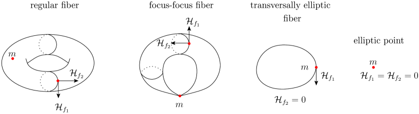
Figure 6: The figures show some possible singularities of a integrable system. On the left most figure, $m$ is a regular point (rank 2); on the second figure, $m$ is a focus-focus point (rank $0$); on the third one, $m$ is a transversally elliptic singularity (rank $1$); on the right most figure, $m$ is an elliptic-elliptic point (rank 0).

Theorem 2.3 (H. Eliasson 1990).

The non-degenerate critical points of a completely integrable system $F\colon M\to\mathbb{R}^{n}$ are linearizable, i.e. if $m\in M$ is a non-degenerate critical point of the completely integrable system $F=(f_{1},\,\ldots,f_{n}):M\rightarrow\mathbb{R}^{n}$ then there exist local symplectic coordinates $(x_{1},\,\ldots,x_{n},\,\xi_{1},\,\ldots,\,\xi_{n})$ about $m$, in which $m$ is represented as $(0,\,\ldots,\,0)$, such that $\{f_{i},\,q_{j}\}=0$, for all indices $i,\,j$, where we have the following possibilities for the components $q_{1},\,\ldots,\,q_{n}$, each of which is defined on a small neighborhood of $(0,\,\ldots,\,0)$ in $\mathbb{R}^{n}$:

• Elliptic component: $q_{j}=(x_{j}^{2}+\xi_{j}^{2})/2$, where $j$ may take any value $1\leq j\leq n$.

• Hyperbolic component: $q_{j}=x_{j}\xi_{j}$, where $j$ may take any value $1\leq j\leq n$.

• Focus-focus component: $q_{j-1}=x_{j-1}\,\xi_{j}-x_{j}\,\xi_{j-1}$ and $q_{j}=x_{j-1}\,\xi_{j-1}+x_{j}\,\xi_{j}$ where $j$ may take any value $2\leq j\leq n-1$ (note that this component appears as “pairs”).

• Non-singular component: $q_{j}=\xi_{j}$, where $j$ may take any value $1\leq j\leq n$.

Moreover if $m$ does not have any hyperbolic component, then the system of commuting equations $\{f_{i},\,q_{j}\}=0$, for all indices $i,\,j$, may be replaced by the single equation

$$(F-F(m))\circ\varphi=g\circ(q_{1},\,\ldots,\,q_{n}),$$

where $\varphi=(x_{1},\,\ldots,x_{n},\,\xi_{1},\,\ldots,\,\xi_{n})^{-1}$ and $g$ is a diffeomorphism from a small neighborhood of the origin in $\mathbb{R}^{n}$ into another such neighborhood, such that $g(0,\,\ldots,\,0)=(0,\,\ldots,\,0)$.

If the dimension of $M$ is $4$ and $F$ has no hyperbolic singularities – which is the case we treat in this paper – we have the following possibilities for the map $(q_{1},\,q_{2})$, depending on the rank of the critical point:

• if $m$ is a critical point of $F$ of rank zero, then $q_{j}$ is one of

  • $q_{1}=(x_{1}^{2}+\xi_{1}^{2})/2$ and $q_{2}=(x_{2}^{2}+\xi_{2}^{2})/2$.

  • $q_{1}=x_{1}\xi_{2}-x_{2}\xi_{1}$ and $q_{2}=x_{1}\xi_{1}+x_{2}\xi_{2}$;    on the other hand,

• if $m$ is a critical point of $F$ of rank one, then

  • $q_{1}=(x_{1}^{2}+\xi_{1}^{2})/2$ and $q_{2}=\xi_{2}$.

In this case, a non-degenerate critical point is respectively called elliptic-elliptic, focus-focus, or transversally-elliptic if both components $q_{1},\,q_{2}$ are of elliptic type, $q_{1},\,q_{2}$ together correspond to a focus-focus component, or one component is of elliptic type and the other component is $\xi_{1}$ or $\xi_{2}$, respectively.

Similar definitions hold for transversally-hyperbolic, hyperbolic-elliptic and hyperbolic-hyperbolic non-degenerate critical points.

Definition 2.4   Suppose that $(M,\omega)$ is a connected symplectic four-manifold. An integrable system $F\colon M\to\mathbb{R}^{2}$ is called almost-toric if all the singularities are non-degenerate without hyperbolic components.

Remark 2.5   Suppose that $(M,\omega)$ is a connected symplectic four-manifold. Let $F\colon M\to\mathbb{R}^{2}$ be an integrable system. If $F$ is a toric integrable system, then $F$ is almost-toric, with only elliptic singularities. This follows from the fact that a torus action is linearizable near a fixed point; see, for instance [16]. $\oslash$

A version of the following result is proven in [49] for almost-toric systems for which the map $F$ is proper. Here we replace the condition of $F$ being proper by the condition that $F(M)$ is a closed subset of $\mathbb{R}^{2}$; this introduces additional subtleties. Our proof here is independent of the argument in [49].

Theorem 2.6.

Suppose that $(M,\omega)$ is a connected symplectic four-manifold. Assume that $F\colon M\to{\mathbb{R}}^{2}$ is an almost-toric integrable system with $B:=F(M)$ closed. Then the set of focus-focus critical values is countable, i.e. we may write it as $\{c_{i}\mid\,i\in I\}$, where $I\subset\mathbb{N}$. Consider the following statements:

• the fibers of $F$ are connected;

• the set $B_{r}$ or regular values of $F$ is connected;

• for any value $c$ of $F$, for any sufficiently small disc $D$ centered at $c$, $B_{r}\cap D$ is connected;

• the set of regular values is $B_{r}=\mathring{B}\setminus\{c_{i}\mid\,i\in I\}$. Moreover, the topological boundary $\partial B$ of $B$ consists precisely of the values $F(m)$, where $m$ is a critical point of elliptic-elliptic or transversally elliptic type.

Then statement (i) implies statement (ii), statement (iii) implies statement (iv), and statement (iv) implies statement (ii).

If in addition $F$ is proper, then statement (i) implies statement (iv).

It is interesting to note that the statement is optimal in that no other implication is true (except (iii)$\Rightarrow$(ii) which is a consequence of the stated implications). This gives an idea of the various pathologies that can occur for an almost-toric system.

Proof of Theorem 2.6.

From the local normal form 2.3, focus-focus critical points are isolated, and hence the set of focus-focus critical points is countable (remember that all our manifolds are second countable). Moreover, the image of a focus-focus point is necessarily in the interior of $B$.

Let us show that

$$B_{r}\subset\mathring{B}\setminus\{c_{i}\mid\,i\in I\}.$$ (1)

This is equivalent to showing that any value in $\partial B$ is a critical value of $F$. Since $B$ is closed, $\partial B\subset B$, so for every $c\in\partial B$ we have that $F^{-1}(c)$ is nonempty. By the Darboux-Carathéodory theorem, the image of a regular point must be in the interior of $B$, therefore $F^{-1}(c)$ cannot contain any regular point: the boundary can contain only singular values.

Since a point in $\partial B$ cannot be the image of a focus-focus singularity, it has to be the image of a transversally elliptic or an elliptic-elliptic singularity.

We now prove the implications stated in the theorem.

${\rm(i)}\Rightarrow{\rm(ii)}$: Since $F$ is almost-toric, the singular fibers are either points (elliptic-elliptic), one-dimensional submanifolds (codimension 1 elliptic) or a stratified manifold of maximal dimension 2 (focus-focus and elliptic). This is because none of the critical fibers can contain regular tori since the fibers are assumed to be connected by hypothesis (i). The only critical values that can appear in one-dimensional families are elliptic and elliptic-elliptic critical values (see Figure 7). The focus- focus singularities are isolated. Therefore the union of all critical fibers is a locally finite union of stratified manifolds of codimension at least 2; therefore this union has codimension at least 2. Hence the complement is connected and therefore its image by $F$ is also connected.

${\rm(iii)}\Rightarrow{\rm(iv)}$: There is no embedded line segment of critical values in the interior of $B$ (which would come from codimension 1 elliptic singularities) because this is in contradiction with the hypothesis of local connectedness (iii). Therefore $\mathring{B}\setminus\{c_{i}\mid\,i\in I\}\subset B_{r}$. Hence by (1),

$$\mathring{B}\setminus\{c_{i}\mid\,i\in I\}=B_{r},$$

as desired, and all the elliptic critical values must lie in $\partial B$.

${\rm(iv)}\Rightarrow{\rm(ii)}$: As we saw above, $F^{-1}(\partial B)$ contains only critical points, of elliptic type. Because of the local normal form, the set of rank 1 elliptic critical points in $M$ form a 2-dimensional symplectic submanifold with boundary, and this boundary is equal to the discrete set of rank 0 elliptic points. Therefore $M\setminus F^{-1}(\partial B)$ is connected. This set is equal to $F^{-1}(\mathring{B})$, which in turn implies that $\mathring{B}$ is connected. By hypothesis (iv), this ensures that $B_{r}$ is connected.

Assume for the rest of the proof that $F$ is proper.

${\rm(i)}\Rightarrow{\rm(iv)}$: Assume (iv) does not hold. In view of (1), there exists an elliptic singularity (of rank 0 or 1) $c$ in the interior of $B$. Let $\Lambda$ be the corresponding fiber. Since it is connected, it must entirely consist of elliptic points (this comes from the normal form Theorem 2.3). The normal form also implies that $c$ must be contained in an embedded line segment of elliptic singularities, and the points in a open neighborhood $\Omega$ of $\Lambda$ are sent by $F$ in only one side of this segment. Since $c$ is in the interior of $B$, there is a sequence $c_{k}\in B$ on the other side of the line segment that converges to $c$ as $k\to\infty$. Hence there is a sequence $m_{k}\in M\setminus\Omega$ such that $F(m_{k})=c_{k}$. Since $F$ is proper, one can assume that $m_{k}$ converges to a point $m$ (necessarily in $M\setminus\Omega$). By continuity of $F$, $m$ belongs to the fiber over $c$, and thus to $\Omega$, which is a contradiction.

∎

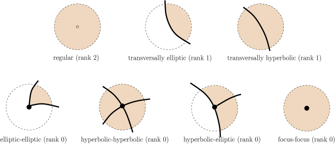
Figure 7: The local classification of the range of $F$ in an open disk.

3 The fibers of an almost-toric system

In this section we study the structure of the fibers of an almost-toric system.

We shall need below the definition and basic properties of the bifurcation set of a smooth map.

Definition 3.1   Let $M$ and $N$ be smooth manifolds. A smooth map $f:M\rightarrow N$ is said to be locally trivial at $n_{0}\in f(M)$ if there is an open neighborhood $U\subset N$ of $n_{0}$ such that $f^{-1}(n)$ is a smooth submanifold of $M$ for each $n\in U$ and there is a smooth map $h:f^{-1}(U)\rightarrow f^{-1}(y_{0})$ such that $f\times h:f^{-1}(U)\rightarrow U\times f^{-1}(n_{0})$ is a diffeomorphism. The bifurcation set $\Sigma_{f}$ consists of all the points of $N$ where $f$ is not locally trivial.

Note, in particular, that $h|_{f^{-1}(n)}:f^{-1}(n)\rightarrow f^{-1}(n_{0})$ is a diffeomorphism for every $n\in U$. Also, the set of points where $f$ is locally trivial is open in $N$.

Remark 3.2   Recall that $\Sigma_{f}$ is a closed subset of $N$. It is well known that the set of critical values of $f$ is included in the bifurcation set (see [1, Proposition 4.5.1]). In general, the bifurcation set strictly includes the set of critical values. This is the case for the momentum-energy map for the two-body problem [1, §9.8]. However (see [1, Page 340]), if $f\colon M\to N$ is a smooth proper map, then the bifurcation set of $f$ is equal to the set of critical values of $f$. $\oslash$

Recall that a smooth map $f:M\rightarrow\mathbb{R}$ is Morse if all its critical points are non-degenerate. The smooth map $f$ is Morse-Bott if the critical set of $f$ is a disjoint union of connected submanifolds $\mathcal{C}_{i}$ of $M$, on which the Hessian of $f$ is non-degenerate in the transverse direction, i.e.,

$$\ker(\operatorname{Hess}_{m}f)={\rm T}_{m}\mathcal{C}_{i},\,\,\,\textup{for all}\,\,i,\,\,\textup{for all}\,\,m\in\mathcal{C}_{i}.$$

The index of $m$ is the number of negative eigenvalues of $(\operatorname{Hess}f)(m)$.

The goal of this section is to find a useful Morse theoretic result, valid in great generality and interesting on its own, that will ultimately imply the connectedness of the fibers of an integrable system (see Theorem 3.7). Here we do not rely on Fomenko’s Morse theory [22], because we do not want to select a nonsingular energy surface. Instead, the model is [36, Lemma 5.51]; however, the proof given there does not extend to the non-compact case, as far as we can tell. We thank Helmut Hofer and Thomas Baird for sharing their insights on Morse theory with us that helped us in the proof of the following result.

Lemma 3.3.

Let $f:M\rightarrow\mathbb{R}$ be a Morse-Bott function on a connected manifold $M$. Assume $f$ is proper and bounded from below and has no critical manifold of index 1. Then the set of critical points of index 0 is connected.

Proof.

We endow $M$ with a Riemannian metric. The negative gradient flow of $f$ is complete. Indeed, along the the flow the function $f$ cannot increase and, by hypothesis, $f$ is bounded from below. Therefore, the values of $f$ remain bounded along the flow. By properness of $f$, the flow remains in a compact subset of $M$ and hence it is complete.

Let us show, using standard Morse-Bott theory, that the integral curve of $-\nabla f$ starting at any point $m\in M$ tends to a critical manifold of $f$. In the compact set in $\{x\in M\mid f(x)\leqslant f(m)\}$, there must be a finite number of critical manifolds contained . If the integral curve avoids a neighborhood of these critical manifolds, by compactness it has a limit point, and by continuity the vector field at the limit point must vanish; we get a contradiction, thus proving the claim.

Thus, we have the disjoint union $M=\bigsqcup_{k=0}^{n}W^{s}(C_{k})$, where $C_{k}$ is the set of critical points of index $k$, and $W^{s}(C_{k})$ is its stable manifold:

$$W^{s}(C_{k}):=\{m\in M\mid d(\varphi_{-\nabla f}^{t}(m),C_{k})\rightarrow 0\text{ as }t\rightarrow+\infty\},$$

where $d$ is any distance compatible with the topology of $M$ (for example, the one induced by the given Riemannian metric on $M$) and $t\mapsto\varphi_{-\nabla f}^{t}$ is the flow of the vector field $-\nabla f$. Since $f$ has no critical point of index 1, we have

$$C_{0}=W^{s}(C_{0})=M\setminus\bigsqcup_{k=2}^{n}W^{s}(C_{k}).$$

The local structure of Morse-Bott singularities given by the Morse-Bott lemma [4, 7]) implies that $W^{s}(C_{k})$ is a submanifold of codimension $k$ in $M$. Hence $\bigsqcup_{k=2}^{n}W^{s}(C_{k})$ cannot disconnect $M$. ∎

Remark 3.4   Since all local minima of $f$ are in $C_{0}$, we see that $C_{0}$ must be the set of global minima of $f$; thus $C_{0}$ must be equal to the level set $f^{-1}(f(C_{0}))$. $\oslash$

Proposition 3.5.

Let $M$ be a connected smooth manifold and $f:M\rightarrow\mathbb{R}$ be a proper Morse-Bott function whose indices and co-indices are always different from 1. Then the level sets of $f$ are connected.

Proof.

Let $c$ be a regular value of $f$ (such a value exists by Sard’s theorem). Then $g:=(f-c)^{2}$ is a Morse-Bott function. On the set $\{x\in M\mid f(x)>c\}$, the critical points of $g$ coincide with the critical points of $f$ and they have the same index. On the set $\{x\in M\mid f(x)<c\}$, the critical points of $g$ also coincide with the critical points of $f$ and they have the same coindex. The level set $\{x\in M\mid f(x)=c\}$ is clearly a set of critical points of index 0 of $g$. Of course, $g$ is bounded from below. Thus, by Lemma 3.3, the set of critical points of index 0 of $g$ is connected (it may be empty) and hence equal to $g^{-1}(0)$. Therefore $f^{-1}(c)$ is connected. This shows that all regular level sets of $f$ are connected. (As usual, a regular level set — or regular fiber — is a level set that contains only regular points, i.e. the preimage of a regular value.)

Finally let $c_{i}$ be a critical value of $f$ (if any). Since $f$ is proper and has isolated critical manifolds, the set of critical values is discrete. Let $\epsilon_{0}>0$ such that the interval $[c_{i}-\epsilon_{0},c_{i}+\epsilon_{0}]$ does not contain any other critical value. Consider the manifold $N:=M\times S^{2}$, and, for any $\epsilon\in(0,\epsilon_{0})$, let

$$h_{\epsilon}:=f-c_{i}+\epsilon z:N\rightarrow\mathbb{R},$$

where $z$ is the vertical component on the sphere $S^{2}\subset\mathbb{R}^{3}$. Notice that $z:S^{2}\rightarrow\mathbb{R}$ is a Morse function with indices 0 and 2. Thus $h_{\epsilon}$ is a Morse-Bott function on $N$ with indices and coindices of the same parity as those of $f$. Thus no index nor coindex of $h$ can be equal to 1. By the first part of the proof, the regular level sets of $h_{\epsilon}$ must be connected. The definition of $\epsilon_{0}$ implies that $0$ is a regular value of $h_{\epsilon}$. Thus

$$F_{\epsilon}:=\pi_{M}(h_{\epsilon}^{-1}(0))=\{m\in M\mid\quad\left|f(m)-c_{i}\right|\leqslant\epsilon\}$$

is connected. Since $f$ is proper, $F_{\epsilon}$ is also compact. Because a non-increasing intersection of compact connected sets is connected, we see that $f^{-1}(c_{i})=\cap_{0<\epsilon\leqslant\epsilon_{0}}F_{\epsilon}$ is connected. ∎

There is no a priori reason why the fibers $F^{-1}(x,\,y)=J^{-1}(x)\cap H^{-1}(y)$ of $F$ should be connected even if $J$ and $H$ have connected fibers (let alone if just one of $J$ or $H$ has connected fibers). However, the following result shows that this conclusion is holds. To prove it, we need a preparatory lemma which is interesting on its own.

Lemma 3.6.

Let $f:X\to\mathbb{R}^{n}$ be a map from a smooth connected manifold $X$ to $\mathbb{R}^{n}$. Ler $B_{r}$ be the set of regular values of $f$. Suppose that $f$ has the following properties.

• $f$ is a proper map.

• For every sufficiently small neighborhood $D$ of any critical value of $f$, $B_{r}\cap D$ is connected.

• The regular fibers of $f$ are connected.

• The set $\mathrm{Crit}(f)$ of critical points of $f$ has empty interior.

Then the fibers of $f$ are connected.

Proof.

We use the following “fiber continuity” fact : that if $\Omega$ is a neighborhood of a fiber $f^{-1}(c)$ of a continuous proper map $f$, then the fibers $f^{-1}(q)$ with $q$ close to $c$ also lie inside $\Omega$. Indeed, if this statement were not true, then there would exist a sequence $q_{n}\rightarrow c$ and a sequence of points $x_{n}\in f^{-1}(q_{n})$, $x_{n}\notin\Omega$, such that there is a subsequence $x_{n_{k}}\rightarrow x\notin\Omega$. However, by continuity $x\in f^{-1}(c)$ which is a contradiction.

Assume a fiber $\mathcal{F}=f^{-1}(p)$ of $f$ is not connected. Then there are disjoint open sets $U$ and $V$ in $X$ such that $\mathcal{F}$ lies in $U\cup V$ but is not contained in either $U$ or $V$.

By fiber continuity, there exists a small open disk $D$ about $p$ such that $f^{-1}(D)\subset U\cup V$.

Since the regular fibers are connected, we can define a map $\psi:D\cap B_{r}\to\{0;1\}$ which for $c\in D\cap B_{r}$ is equal to $1$ if $f^{-1}(c)\subset U$, and is equal to $0$ if $f^{-1}(c)\subset V$. The fiber continuity says that the sets $\psi^{-1}(0)$ and $\psi^{-1}(1)$ are open, thus proving that $\psi$ is continuous. By (2), the image of $\psi$ must be connected, and therefore $\psi$ is constant. We can hence assume without loss of generality that all regular fibers above $D$ are contained in $U$.

Now consider the restriction $\tilde{f}$ of $f$ on the open set $V\cap f^{-1}(D)$. Because of the above argument, it cannot take any value in $B_{r}\cap D$. Thus this map takes values in the set of critical values of $f$, which has measure zero by Sard’s theorem. This requires that on $V\cap f^{-1}(D)$, the rank of $\mathrm{d}f$ be strictly less that $n$, which contradicts (4), and hence proves the lemma : $f^{-1}(p)$ has to be connected. ∎

Now we are ready to prove one of our main results.

Theorem 3.7.

Suppose that $(M,\omega)$ is a connected symplectic four-manifold. Let $F=(J,\,H)\colon M\to\mathbb{R}^{2}$ be an almost-toric integrable system such that $F$ is a proper map. Suppose that $J$ has connected fibers, or that $H$ has connected fibers. Then the fibers of $F$ are connected.

Proof.

Without loss of generality, we may assume that $J$ has connected fibers.

Step 1.

We shall prove first that for every regular value $(x,\,y)$ of $F$, the fiber $F^{-1}(x,\,y)$ is connected. To do this, we divide the proof into two cases.

Case 1A. Assume $x$ is a regular value of $J$. Then the fiber $J^{-1}(x)$ is a smooth manifold. Let us show first that the non-degeneracy of the critical points of $F$ and the definition of almost-toric systems implies that the function $H_{x}:=H|_{J^{-1}(x)}\colon J^{-1}(x)\to\mathbb{R}$ is Morse-Bott. Let $B_{r}$ be the set of regular values of $F$.

Let $m_{0}$ be a critical point of $H_{x}$. Then there exists $\lambda\in\mathbb{R}$ such that $\mathrm{d}H(m_{0})=\lambda\mathrm{d}J(m_{0})$. Thus $m_{0}$ is a critical point of $F$; it must be of rank $1$ since $\mathrm{d}J$ never vanishes on $J^{-1}(x)$. Since $F$ is an almost-toric system, the only possible rank $1$ singularities are transversally elliptic singularities, i.e., singularities with one elliptic component and one non singular component in Theorem 2.3; see Figure 7. Thus, by Theorem 2.3, there exist local canonical coordinates $(x_{1},\,x_{2},\,\xi_{1},\,\xi_{2})$ such that $F=g(x_{1}^{2}+\xi_{1}^{2},\,\xi_{2})$ for some local diffeomorphism $g$ of $\mathbb{R}^{2}$ about the origin and fixing the origin; thus the derivative

$${\rm D}g(0,0)=:\begin{pmatrix}a&b\\ c&d\end{pmatrix}\in\operatorname{GL}(2,\mathbb{R}).$$

Note $\mathrm{d}J(m_{0})\neq 0$ implies that $d\neq 0$. Therefore, by the implicit function theorem, the submanifold $J^{-1}(x)$ is locally parametrized by the variables $(x_{1},x_{2},\xi_{1})$ and, within it, the critical set of $H_{x}$ is given by the equation $x_{1}=\xi_{1}=0$; this is a submanifold of dimension 1. The Taylor expansion of $H_{x}$ is easily computed to be

$$H_{x}=a(x_{1}^{2}+\xi_{1}^{2})-\frac{bc}{d}(x_{1}^{2}+\xi_{1}^{2})+\frac{b}{d}x+\mathcal{O}(x_{1},\xi_{1},x_{2})^{3}.$$ (2)

Thus, the coefficient of $(x_{1}^{2}+\xi_{1}^{2})$ is $(a-\frac{bc}{d})$ which is non-zero and hence the Hessian of $H_{x}$ is transversally non-degenerate. This proves that $H_{x}$ is Morse-Bott, as claimed.

Second, we prove, in this case, that the fibers of $F$ are connected. At $m_{0}$, the transversal Hessian of $H_{x}$ has either no or two negative eigenvalues, depending on the sign of $(a-\frac{bc}{d})$. This implies that each critical manifold has index $0$ or index $2$. If this coefficient is negative, the sum of the two corresponding eigenspaces is the full $2$-dimensional $(x_{1},\xi_{1})$-space.

Note that $H_{x}\colon J^{-1}(x)\to\mathbb{R}$ is a proper map: indeed, if $K\subset\mathbb{R}$ is compact, then $H_{x}^{-1}(K)=F^{-1}(\{x\}\times K)$ is compact because $F$ is proper. Thus $H_{x}\colon J^{-1}(x)\to\mathbb{R}$ is a smooth Morse-Bott function on the connected manifold $J^{-1}(x)$ and $H_{x}$ and $-H_{x}$ have only critical points of index $0$ or $2$. We are in the hypothesis of Proposition 3.5 and so we can conclude that the fibers of $H_{x}\colon J^{-1}(x)\to\mathbb{R}$ are connected.

Now, since $(H_{x})^{-1}(y)=F^{-1}(x,\,y)$, it follows that $F^{-1}(x,\,y)$ is connected for all $(x,\,y)\in F(M)\subset\mathbb{R}^{2}$ whenever $x$ is a regular value of $J$.

Case 1B. Assume that $x$ is not a regular value of $J$. Note that there exists a point $(a,\,b)$ in every connected component $C_{r}$ of $B_{r}$ such that $b$ is a regular value for $J$; otherwise $\mathrm{d}J$ would vanish on $F^{-1}(C_{r})$, which violates the definition of $B_{r}$. The restriction $F|_{F^{-1}(C_{r})}\colon F^{-1}(C_{r})\to C_{r}$ is a locally trivial fibration since, by assumption, $F$ is proper and thus the bifurcation set is equal to the critical set. Thus all fibers of $F|_{F^{-1}(C_{r})}$ are diffeomorphic. It follows that $F^{-1}(x,\,y)$ is connected for all $(x,\,y)\in C_{r}$.

This shows that all inverse images of regular values of $F$ are connected.

Step 2.

We need to show that $F^{-1}(x,y)$ is connected if $(x,y)$ is not a regular value of $F$. We claim that there is no critical value of $F$ in the interior of the image $F(M)$, except for the critical values that are images of focus-focus critical points of $F$. Indeed, if there was such a critical value $(x_{0},\,y_{0})$, then there must exist a small segment line $\ell$ of critical values (by the local normal form described in Theorem 2.3 and Figure 7). Now we distinguish two cases.

Case 2A. First assume that $\ell$ is not a vertical segment (i.e., contained in a line of the form $x=\textup{constant}$) and let $\hat{\ell}:=F^{-1}(\ell)$. Then $J(\hat{\ell})$ contains a small interval around $x$, so by Sard’s theorem, it must contain a regular value $x_{0}$ for the map $J$. Then $J^{-1}(x_{0})$ is a smooth manifold which is connected, by hypothesis. By the argument earlier in the proof (see Step 1, Case A), both $H$ and $-H$ restricted to $J^{-1}(x_{0})$ are proper Morse-Bott functions with indices $0$ and $2$. So, if there is a local maximum or local minimum, it must be unique. However, the existence of this line of rank 1 elliptic singularities implies that there is a local maximum/minimum of $H_{x_{0}}$ (see formula (2)). Since the corresponding critical value lies in the interior of the image of $H_{x_{0}}$, it cannot be a global extremum; we arrived at a contradiction. Thus the small line segment $\ell$ must be vertical.

Case 2B. Second, suppose that $\ell$ is a vertical segment (i.e., contained in a line of the form $x=\textup{constant}$) and let $\hat{\ell}:=F^{-1}(\ell)$. We can assume, without loss of generality, that the connected component of $\ell$ in the bifurcation set is vertical in the interior of $F(M)$; indeed, if not, apply Case 2A a above.

From Figure 7 we see that $\hat{\ell}$ must contain at least one critical point $A$ of transversally elliptic type together with another point $B$ either regular or of transversally elliptic type. By the normal form of non-degenerate singularities, $J^{-1}(x_{0})$ must be locally path connected. Since it is connected by assumption, it must be path connected. So we have a path $\gamma:[0,1]\mapsto J^{-1}(x_{0})$ such that $\gamma(0)=A$ and $\gamma(1)=B$. Near $A$ we have canonical coordinates $(x_{1},x_{2},\xi_{1},\xi_{2})\in\mathbb{R}^{4}$ and a local diffeomorphism $g$ defined in a neighborhood of the origin of $\mathbb{R}^{2}$ and preserving it, such that

$$F=g(x_{1}^{2}+\xi_{1}^{2},\xi_{2})$$

and $A=(0,0,0,0)$. Write $g=(g_{1},g_{2})$. The critical set is defined by the equations $x_{1}=\xi_{1}=0$ and, by assumption, is mapped by $F$ to a vertical line. Hence $g_{1}(0,\xi_{2})$ is constant, so

$$\partial_{2}g_{1}(0,\xi_{2})=0.$$

Since $g$ is a local diffeomorphism, $\mathrm{d}g_{1}\neq 0$, so we must have $\partial_{1}g_{1}\neq 0$. Thus, by the implicit function theorem, any path starting at $A$ and satisfying $g_{1}(x_{1}^{2}\xi_{1}^{2},\xi_{2})=\text{constant}$ must also satisfy $x_{1}^{2}+\xi_{1}^{2}=0$. Therefore, $\gamma$ has to stay in the critical set $x_{1}=\xi_{1}=0$.

Assume first that $\gamma([0,1])$ does not touch the boundary of $F(M)$. Then this argument shows that the set of $t\in[0,1]$ such that $\gamma(t)$ belongs to the critical set of $F$ is open. It is also closed by continuity of $\mathrm{d}F$. Hence it is equal to the whole interval $[0,1]$. Thus $B$ must be in the critical set; this rules out the possibility for $B$ to be regular. Thus $B$ must be a rank-1 elliptic singularity. Notice that the sign of $\partial_{1}g_{1}$ indicates on which side of $\ell$ (left or right) lie the values of $F$ near $A$.

Thus, even if $g_{1}$ itself is not globally defined along the path $\gamma$, this sign is locally constant and thus globally defined along $\gamma$. Therefore, all points near $\hat{\ell}$ are mapped by $F$ to the same side of $\ell$, which says that $\ell$ belongs to the boundary of $F(M)$; this is a contradiction.

Finally, assume that $\gamma([0,1])$ touches the boundary of $F(M)$. From the normal form theorem, this can only happen when the fiber over the contact point contains an elliptic-elliptic point $C$. Thus there are local canonical coordinates $(x_{1},x_{2},\xi_{1},\xi_{2})\in\mathbb{R}^{4}$ and a local diffeomorphism $g$ defined in a neighborhood of the origin of $\mathbb{R}^{2}$ and preserving it, such that

$$F=g(x_{1}^{2}+\xi_{1}^{2},x_{2}^{2}+\xi_{2}^{2})$$

near $C=(0,0,0,0)$. We note that the same argument as above applies: simply replace the $\xi_{2}$ component by $x_{2}^{2}+\xi_{2}^{2}$. Thus we get another contradiction. Therefore there are no critical values $c$ in the interior of the image $F(M)$ other than focus-focus values (i.e., images of focus-focus points).

Step 3.

We claim here that for any critical value $c$ of $F$ and for any sufficiently small disk $D$ centered at $c$, $B_{r}\cap D$ is connected.

First we remark that Step 2 implies that item (iv) in Theorem 2.6 holds, and hence item (ii) must hold : the set of regular values of $F$ is connected.

If $c$ is a focus-focus value, it must be contained in the interior of $F(M)$, therefore it follows from Step 2 that it is isolated : there exists a neighborhood of $c$ in which $c$ is the only critical value, which proves the claim in this case.

We assume in the rest of the proof that $c=(x_{c},y_{c})$ is an elliptic (of rank 0 or 1) critical value of $F$. Since we have just proved in Step 2 that there are no critical values in the interior of $F(M)$ other than focus-focus values, we conclude that $c\in\partial(F(M))$. Moreover, the fiber cannot contain a regular Liouville torus. Then, again by Theorem 2.3, the only possibilities for a neighborhood of $c$ in $F(M)$ are superpositions of elliptic local normal forms of rank 0 or 1 (given by Theorem 2.3) in such a way that $c\in\partial(F(M))$. If only one local model appears, then the claim is immediate.

Let us show that a neighborhood $U$ of $c$ cannot contain several different images of local models. Indeed, consider the possible configurations for two different local images $C_{1}$ and $C_{2}$: either both $C_{1}$ and $C_{2}$ are elliptic-elliptic images, or both are transversally elliptic images, or $C_{1}$ is an elliptic-elliptic image and $C_{2}$ is a transversally elliptic image. Step 2 implies that the critical values of $F$ in $C_{1}$ and $C_{2}$ can only intersect at a point, provided the neighborhood $U$ is taken to be small enough. Let us consider a vertical line $\ell$ through $C_{1}$ which corresponds to a regular value of $J$. Any crossing of $\ell$ with a non-vertical boundary of $F(M)$ must correspond to a local extremum of $H|_{F^{-1}(\ell)}$, and by Step 2 this local extremum has to be a global one. Since only one global maximum and one global minimum are possible, the only allowed configurations for $C_{1}$ and $C_{2}$ are such that the vertical line $\ell_{c}$ through $c$ separates the regular values of $C_{1}$ from the regular values of $C_{2}$ (see Figure 8).

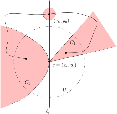
Figure 8: Point overlapping of images near singularities. Such a situation cannot occur if the fibers of $J$ are connected.

Since $B_{r}$ is path connected, there exists a path in $B_{r}$ connecting a point in $B_{r}\cap C_{1}$ to a point in $B_{r}\cap C_{2}$. By continuity this path needs to cross $\ell_{c}$, and the intersection point $(x_{0}=x_{c},y_{0})$ must lie outside $U$. Therefore there exists an open ball $B_{0}\subset B_{r}$ centered at $(x_{0},y_{0})$. Suppose for instance that $y_{0}>y_{c}$. Then for $(x,y)\in U$, $y$ cannot be a maximal value of $H|_{J^{-1}(x)}$, which means that for each of $C_{1}$ and $C_{2}$, only local minima for $H|_{J^{-1}(x)}$ are allowed. This cannot be achieved by any of the local models, thus finishing the proof of our claim.

The statement of the theorem now follows from Lemma 3.6 since all fibers are codimension at least one (this follows directly from the independence assumption in the definition of an integrable system. But, in fact, we know from the topology of non-degenerate integrable systems that fibers have codimension at least two [8]). ∎

Remark 3.8   It is not true that an almost-toric integrable system with connected regular fibers has also connected singular fibers. See example 8 below. $\oslash$

The following are examples of almost-toric systems in which the fibers of $F$ are not connected. In the next section we will combine Theorem 3.7 with an upcoming result on contact theory for singularities (which we will prove too) in order to obtain Theorem 2 of Section 1.

Example 3.9   This example appeared in [48, Chapter 5, Figure 29]. It is an example of a toric system $F:=(J,\,H)\colon M\to\mathbb{R}^{2}$ on a compact manifold for which $J$ and $H$ have some disconnected fibers (the number of connected components of the fibers also changes). Because this example is constructed from the standard toric system $S^{2}\times S^{2}$ by precomposing with a local diffeomorphism, the singularities are non-degenerate. In this case the fundamental group $\pi_{1}(F(M))$ has one generator, so $F(M)$ is not simply connected, and hence not contractible. See Figure 9. An extreme case of this example can be obtained by letting only two corners overlap (Figure 10). We get then an almost-toric system where all regular fibers are connected, but one singular fiber is not connected. $\oslash$

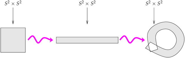
Figure 9: An almost-toric system with some disconnected fibers, constructed from the standard toric system on $S^{2}\times S^{2}$ by precomposing with a local diffeomorphism.

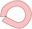
Figure 10: Image of integrable system constructed from $S^{2}\times S^{2}$ by a one-point identification, and which has one disconnected fiber. All the other fibers are connected.

Example 3.10   The manifold is $M:=S^{2}\times S^{1}\times S^{1}$. Choose coordinates $h\in[1,\,2]$, $a\in\mathbb{R}/2\pi\mathbb{Z}$ on $S^{2}$; these are action-angle coordinates for the Hamiltonian system given by the rotation action. Choose coordinates $b,c\in\mathbb{R}/2\pi\mathbb{Z}$ on $S^{1}\times S^{1}$. For each $n\in\mathbb{N}$, $n\neq 0$, the 2-form $\mathrm{d}h\wedge\mathrm{d}a+n\mathrm{d}b\wedge\mathrm{d}c$ is symplectic. Let

$$F(h,\,a,\,b,\,c):=(J:=h\cos(nb),\,H:=h\sin(nb))$$

and note that $J$ is the momentum map of an $S^{1}$-action rotating the sphere about the vertical axis and the first component of $S^{1}\times S^{1}$.

Note that $F$ maps $M$ onto the annulus in Figure 11.

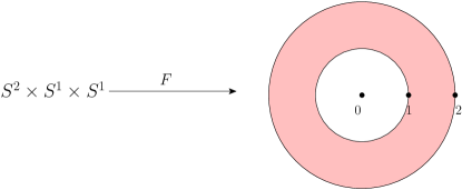
Figure 11: An almost toric system with disconnected fibers.

Topologically $F$ winds the first copy of $S^{1}$ exactly $n$ times around the annulus and maps $S^{2}$ to radial intervals. The fiber of any regular value is thus $n$ copies of $(S^{1})^{2}$, while the preimage of any singular value is $S^{1}$. One can easily check that all singular fibers are transversely elliptic. The Hamiltonian vector fields are:

$$\mathcal{H}_{J}=\cos(nb)\frac{\partial}{\partial a}-h\sin(nb)\frac{\partial}{\partial c},\,\,\,\,\,\,\mathcal{H}_{H}=\sin(nb)\frac{\partial}{\partial a}+h\cos(nb)\frac{\partial}{\partial c}$$

which are easily checked to commute (the coefficient functions are invariants of the flow). Observe that neither integrates to a global circle action. As for the components, they all look alike (the system has rotational symmetry in the $b$ coordinate). Consider for instance the component $J(h,a,b,c)=h\cos(nb)$ which has critical values $-2,-1,1,2$ and is Morse-Bott with critical sets equal to $n$ copies of $S^{1}$ and with Morse indices $0,2,1$, and $3$, respectively. The sets $J<-2$ and $J>2$ are empty. For any $-2<k<-1$ or $1<k<2$, the fiber of $J^{-1}(k)$ is equal to $n$ copies of $S^{2}\times S^{1}$ and for $-1<k<1$ the fiber $J^{-1}(k)$ is equal to $2n$ copies of $S^{2}\times S^{1}$. We thank Thomas Baird for this example. $\oslash$

Remark 3.11   Much of our interest on this topic came from questions asked by physicists and chemists in the context of molecular spectroscopy [40, Section 1], [21, 43, 13, 2]. Many research teams have been working on this topic, to name a few: Mark Child’s group in Oxford (UK), Jonathan Tennyson’s at the University College London (UK), Frank De Lucia’s at Ohio State University (USA), Boris Zhilinskii’s at Dunkerque (France), and Marc Joyeux’s at Grenoble (France).

For applications to concrete physical models the theorem is far reaching.

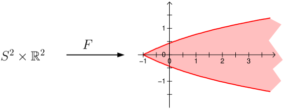
Figure 12: Coupled-spin oscillator

The reason is that is essentially impossible to prove connectedness of the fibers of concrete physical systems. For the purpose of applications, a computer may approximate the bifurcation set of a system and find its image to a high degree of accuracy. See for example the case of the coupled spin-oscillator in Figure 12, which is one of the most fundamental examples in classical physics, and which recently has attracted much attention, see [5, 6]. $\oslash$

4 The image of an almost-toric system

In this section we study the structure of the image of an almost-toric system.

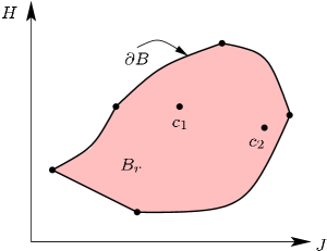
Figure 13: The image $B:=F(M)$ of an almost-toric momentum map $F=(J,\,H)\colon M\to{\mathbb{R}}^{2}$. The set of regular values of $F$ is denoted by $B_{r}$. The marked dots $c_{1},\,c_{2}$ inside of $B$ represent singular values, corresponding to the focus-focus fibers. The set $B_{r}$ is equal to $B$ minus $\partial B\cup\{c_{1},\,c_{2}\}$.

4.1 Images bounded by lower/upper semicontinuous graphs

We star with the following observation.

Lemma 4.1.

Let $M$ be a connected smooth manifold and let $f\colon M\to\mathbb{R}$ be a Morse-Bott function with connected fibers. Then the set $C_{0}$ of index zero critical points of $f$ is connected. Moreover, if $\lambda_{0}:=\inf f\geqslant-\infty$, the following hold:

• If $\lambda_{0}>-\infty$ then $C_{0}=f^{-1}(\lambda_{0})$.

• If $\lambda_{0}=-\infty$ then $C_{0}=\varnothing$.

Proof.

The fiber over a point is locally path connected. If the point is critical this follows from the Morse-Bott Lemma and if the point is regular, this follows from the submersion theorem.

Let $m$ be a critical point of index $0$ of $f$, i.e., $m\in C_{0}$, and let $\lambda:=f(m)$, $\Lambda:=f^{-1}(\lambda)$. Let $\gamma\colon[0,\,1]\to\Lambda$. Since $\Lambda$ is connected and locally path connected, it is path connected. Let $\gamma\colon[0,\,1]\to\Lambda$ be a continuous path starting at $m$. By the Morse-Bott Lemma, $\operatorname{im}(\gamma)\subset C_{0}$. Therefore, since $\Lambda$ is path connected, $\Lambda\subseteq C_{0}$. Each connected component of $C_{0}$ is contained in some fiber of $f$ and hence $\Lambda$ is the connected component of $C_{0}$ that contains $m$. We shall prove that $C_{0}$ has one one connected component.

Assume that there is a point $m^{\prime}$ such that $f(m^{\prime})<\lambda$ and let $\delta\colon[0,\,1]\to M$ be a continuous path from $m$ to $m^{\prime}$. Let

$$t_{0}:=\inf\{t>0\,|\,f(\delta(t))<\lambda\}.$$

Then $f(\delta(t_{0}))=\lambda$ and, by definition, for every $\alpha>0$ there exists $t_{\alpha}\in[t_{0},\,t_{0}+\alpha]$ such that $f(\delta(t_{\alpha}))<\lambda$.

Let $m_{0}:=\delta(t_{0})$. Let $U$ be a neighborhood of $\delta(t_{0})$ in which we have the Morse-Bott coordinates given by the Morse-Bott Lemma centered at $\delta(t_{0})$. For $\alpha$ small enough, $\delta([t_{0},\,t_{1}])\subset U$ and therefore for $t\in[t_{0},\,t_{1}]$ we have that

$$f(\delta(t))=\sum_{i=1}^{k}y_{i}^{2}(\delta(t))+\lambda\geqslant\lambda,$$

which is a contradiction. ∎

Note that the following result is strictly Morse-theoretic; it does not involve integrable systems. A version of this result was proven in [49, Theorem 3.4] in the case of integrable systems $F=(J,\,H)$ for which $J\colon M\to\mathbb{R}$ is both a proper map (hence $F\colon M\to\mathbb{R}^{2}$ is proper) and a momentum map for a Hamiltonian $S^{1}$-action. The version we prove here applies to smooth maps, which are not necessarily integrable systems.

Theorem 4.2.

Let $M$ be a connected smooth four-manifold. Let $F=(J,\,H)\colon M\to\mathbb{R}^{2}$ be a smooth map. Equip $\overline{\mathbb{R}}:=\mathbb{R}\cup\{\pm\infty\}$ with the standard topology. Suppose that the component $J$ is a non-constant Morse-Bott function with connected fibers. Let $H^{+},\,H^{-}\colon J(M)\to\overline{\mathbb{R}}$ be the functions defined by $H^{+}(x):=\sup_{J^{-1}(x)}H$ and $H^{-}(x):=\inf_{J^{-1}(x)}H$. The functions $H^{+}$, $-H^{-}$ are lower semicontinuous. Moreover, if $F(M)$ is closed in $\mathbb{R}^{2}$ then $H^{+}$, $-H^{-}$ are upper semicontinuous (and hence continuous), and $F(M)$ may be described as

$$F(M)=\!\!\mathop{\rm~{}epi}\nolimits(H^{-})\cap\!\!\mathop{\rm~{}hyp}\nolimits(H^{+}).$$ (3)

In particular, $F(M)$ is contractible.

Proof.

First we consider the case where $F(M)$ is not necessarily closed (Part 1). In Part 2 we prove the stronger result when $F(M)$ is closed.

Part 1.

We do not assume that $F(M)$ is closed and prove that $H^{+}$ is lower semicontinuous; the proof that $H^{-}$ is lower semicontinuous is analogous. Since, by assumption, $J$ is non-constant, the interior set $\operatorname{int}J(M)$ of $J(M)$ is non-empty. The set $\operatorname{int}J(M)$ is an open interval $(a,\,b)$ since $M$ is connected and $J$ is continuous. Lower semicontinuity of $H^{+}$ is proved first in the interior of $J(M)$ (case A) and then at the possible boundary (case B).

Case A. Let $x_{0}\in\operatorname{int}J(M)$, and let $y_{0}:=H^{+}(x_{0})$. Let $\epsilon>0$. By the definition of supremum, there exists $\epsilon^{\prime}>0$ with $\epsilon^{\prime}<\epsilon$ such that if $y_{1}:=y_{0}-\epsilon^{\prime}$ then $F^{-1}(x_{0},\,y_{1})\neq\varnothing$ (see Figure 14). Here we have assumed that $y_{0}<+\infty$; if $y_{0}=+\infty$, we just need to replace $y_{1}$ by an arbitrary large constant. Let $m\in F^{-1}(x_{0},\,y_{1})$. Then $J(m)=x_{0}$. Endow $M$ with a Riemannian metric and, with respect to this metric, consider the gradient vector field $\nabla J$ of $J$. Let $t_{0}>0$ such that the flow $\varphi^{t}(m)$ of $\nabla J$ starting at $\varphi^{0}(m)=m$ exists for all $t\in(-t_{0},\,t_{0})$. Now we distinguish two cases.

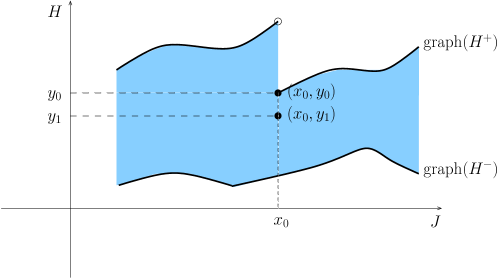
Figure 14: Lower semicontinuity of $H^{+}$.

• Assume $\mathrm{d}J(m)\neq 0$. Since $\nabla J(m)\neq 0$, the set

  $$\Lambda_{t_{0}}:=\{J(\varphi(t))\,|\,t\in(-t_{0},\,t_{0})\}$$

  is a neighborhood of $x_{0}$.

  Let $B$ the ball of radius $\epsilon$ centered at $(x_{0},\,y_{1})$. Let $U:=F^{-1}(B)$, which contains $m$. Let $t^{\prime}_{0}\leqslant t_{0}$ be small enough such that $\varphi^{t}(m)\in U$ for all $|t|<t^{\prime}_{0}$. The set $\Lambda_{t^{\prime}_{0}}$ is a neighborhood of $x_{0}$, so there is $\alpha>0$ such that $(x_{0}-\alpha,\,x_{0}+\alpha)\subseteq\Lambda_{t^{\prime}_{0}}$.

  Let $x\in\Lambda_{t^{\prime}_{0}}$; there exists $|t|<t^{\prime}_{0}$ such that $J(\varphi^{t}(m))=x$ by definition of $\Lambda_{t^{\prime}_{0}}$. Since $F(\varphi^{t}(m))\in B$ we conclude that $y:=H(\varphi^{t}(m))\in(y_{1}-\epsilon,\,y_{1}+\epsilon)$, so $H^{+}(x)\geqslant y\geqslant y_{1}-\epsilon$ for all $x$ with $|x-x_{0}|<\alpha$.

  Thus we get $H^{+}(x)\geqslant y_{0}-2\epsilon$ for all $x$ with $|x-x_{0}|<\alpha$, which proves the lower semicontinuity.

• Assume $\mathrm{d}J(m)=0$. By Lemma 4.1 we conclude that $m$ is not of index $0$, for otherwise $J(m)=x_{0}$ would be a global minimum in $J(M)$ which contradicts the fact that, by assumption, $x_{0}\in\operatorname{int}J(M)$.

  Thus the Hessian of $J$ has at least one negative eigenvalue and therefore there exists $t_{0}>0$ such that $\Lambda_{t_{0}}$ is an open neighborhood of $x_{0}$ and we may then proceed as in Case A.1.

Hence $H^{+}$ is lower semicontinuous.

Case B. We prove here lower semicontinuity at a point $x_{0}$ in the topological boundary of $J(M)$. We may assume that $J(M)=[a,\,b)$ and that $x_{0}=a$. By Lemma 4.1, $J^{-1}(a)=C_{0}$, where $C_{0}$ denotes the set of critical points of $J$ of index $0$. If $m\in J^{-1}(a)$ and $U$ is a small neighborhood of $m$, it follows from the Morse-Bott lemma that $J(U)$ is a neighborhood of $a$ in $J(M)$. Hence we may proceed as in Case A to conclude that $H^{+}$ is lower semicontinuous.

Part 2.

Assuming that $F(M)$ is closed we shall prove now that $H^{+}$ is upper semicontinuous.

Suppose that $H^{+}$ is not upper semicontinuous at some point $x_{0}\in J(M)$ (so we must have $H^{+}(x_{0})<\infty$). Then there exists $\epsilon_{0}>0$ and a sequence $\{x_{n}\}\subset J(M)$ converging to $x_{0}$ such that $H^{+}(x_{n})\geqslant H^{+}(x_{0})+\epsilon_{0}$. First assume that $H^{-}(x_{0})$ is finite. Since $H^{-}$ is upper semicontinuous, for $x$ close to $x_{0}$ we have

$$H^{-}(x)\leqslant H^{-}(x_{0})+\frac{\epsilon_{0}}{2}.$$

Thus we have

$$H^{-}(x_{n})\leqslant H^{-}(x_{0})+\frac{\epsilon_{0}}{2}\leqslant H^{+}(x_{0})+\frac{\epsilon_{0}}{2}<H^{+}(x_{0})+\epsilon_{0}\leqslant H^{+}(x_{n}).$$ (4)

Let $y_{0}\in(H^{+}(x_{0})+\frac{\epsilon_{0}}{2},H^{+}(x_{0})+\epsilon_{0})$. Because of (4), and since $H(J^{-1}(x_{n}))$ is an interval whose closure is $[H^{-}(x_{n}),H^{+}(x_{n})]$ (remember that $J$ has connected fibers and $H$ is continuous), we must have $y_{0}\in H(J^{-1}(x_{n}))$. Therefore $(x_{n},y_{0})\in F(M)$. Since $F(M)$ is closed, the limit of this sequence belongs to $F(M)$; thus $(x_{0},\,y_{0})\in F(M)$. Hence $y_{0}\leqslant H^{+}(x_{0})$, a contradiction. If $H^{-}(x_{0})=-\infty$, we just replace in the proof $H^{-}(x_{0})+\frac{\epsilon_{0}}{2}$ by some constant $A$ such that $A\leqslant H^{+}(x_{0})+\frac{\epsilon_{0}}{2}$.

Hence $H^{+}$ is upper semicontinuous. Therefore $H^{+}$ is continuous. The same argument applies to $H^{-}$.

In order to prove (3), notice that for any $x\in J(M)$, we have the equality

$$\{x\}\times H(J^{-1}(x))=F(M)\cap\{(x,\,y)\,|\,y\in\mathbb{R}\}.$$ (5)

Therefore, if $F(M)$ is closed, $\{x\}\times H(J^{-1}(x))$ must be closed and hence equal to $\{x\}\times[H^{-}(x),H^{+}(x)]$. The equality (3) follows by taking the union of the identity (5) over all $x\in J(M)$.

Finally, we show that $F(M)$ is contractible. Since $\mathbb{R}\cup\{\pm\infty\}$ is homeomorphic to a compact interval, $F(M)$ is homeomorphic to a closed subset of the strip $\mathbb{R}\times[-1,1]$ by means of a homeomorphism $g$ that fixes the first coordinate $x$. Thus, composing (3) by this homeomorphism we get

$$g(F(M))=\text{epi}(h^{-})\cap\text{hyp}(h^{+})$$

for some continuous functions $h^{+}$ and $h^{-}$. Then the map

$$g(F(M))\times[0,1]\ni((x,y),t)\mapsto(x,t(y-h^{-}(x)))\in\mathbb{R}^{2}$$

is a homotopy equivalence with the horizontal axis. Since $g$ is a homeomorphism, we conclude that $F(M)$ is contractible. ∎

4.2 Constructing Morse-Bott functions

We can give a stronger formulation of Theorem 4.2. First, recall that if $\Sigma$ is a smoothly immersed $1$-dimensional manifold in $\mathbb{R}^{2}$, we say that $\Sigma$ has no horizontal tangencies if there exists a smooth curve $\gamma\colon I\subset\mathbb{R}\to\mathbb{R}^{2}$ such that $\gamma(I)=\Sigma$ and $\gamma^{\prime}_{2}(t)\neq 0$ for every $t\in I$. Note that $\Sigma$ has no horizontal tangencies if and only if for every $c\in\mathbb{R}$ the $1$-manifold $\Sigma$ is transverse to the horizontal line $y=c$.

We start with the following result, which is of independent interest and its applicability goes far beyond its use in this paper.

We begin with a description of the structure of the set $\Sigma_{F}:=F(\operatorname{Crit}(F))$ of critical values of an integrable systems $F:M\to\mathbb{R}^{2}$; as usual $\operatorname{Crit}(F)$ denotes the set of critical points of $F$.

Let $c_{0}\in\Sigma_{F}$ and $B\subset\mathbb{R}^{2}$ a small closed ball centered at $c_{0}$. For each point $m\in F^{-1}(B)$ we choose a chart about $m$ in which $F$ has normal form (see Theorem 2.3). There are seven types of normal forms, as depicted in Figure 7. Since $F^{-1}(B)$ is compact, we can select a finite number of such chart domains that still cover $F^{-1}(B)$. For each such chart domain $\Omega$, the set of critical values of $F|_{\Omega}$ is diffeomorphic to the set of critical values of one of the models described in Figure 7, which is either empty, an isolated point, an open curve, or up to four open curves starting from a common point. Since

$$\Sigma_{F}\cap B=F(\textup{Crit}(F)\cap F^{-1}(B)),$$

it follows that $\Sigma\cap B$ is a finite union of such models. This discussion leads to the following proposition.

Proposition 4.3.

Let $(M,\,\omega)$ be a connected symplectic four-manifold. Let $F:M\to\mathbb{R}^{2}$ be a non-degenerate integrable system. Suppose that $F$ is a proper map. Then $\Sigma_{F}:=F(\textup{Crit}(F))$ is the union of a finite number of stratified manifolds with 0 and 1 dimensional strata. More precisely, $\Sigma_{F}$ is a union of isolated points and of smooth images of immersions of closed intervals (since $F$ is proper, a 1-dimensional stratum must either go to infinity or end at a rank-zero critical value of $F$).

Definition 4.4   Let $c\in\Sigma_{F}$. A vector $v\in\mathbb{R}^{2}$ is called tangent to $\Sigma_{F}$ if there is a smooth immersion $\iota:\mathbb{R}\supset[0,1]\to\Sigma_{F}$ with $\iota(0)=c$ and $\iota^{\prime}(0)=v$.

Here $\iota$ is smooth on $[0,1]$, when $[0,1]$ is viewed as a subset of $\mathbb{R}$. Notice that a point $c$ can have several linearly independent tangent vectors.

Definition 4.5   Let $\gamma$ be a smooth curve in $\mathbb{R}^{2}$.

• If $\gamma$ intersects $\Sigma_{F}$ at a point $c$, we say that the intersection is transversal if no tangent vector of $\Sigma_{F}$ at $c$ is tangent to $\gamma$. Otherwise we say that $c$ is a tangency point.

• Assume that $\gamma$ is tangent to a 1-stratum $\sigma$ of $\Sigma_{F}$ at a point $c\in\sigma$. Near $c$, we may assume that $\gamma$ is given by some equation $\varphi(x,y)=0$, where $\mathrm{d}\varphi(c)\neq 0$.

  We say that $\gamma$ has a non-degenerate contact with $\sigma$ at $c$ if, whenever $\delta:(-1,1)\to\sigma$ is a smooth local parametrization of $\sigma$ near $c$ with $\delta(0)=c$, then the map $t\mapsto(\varphi\circ\delta)(t)$ has a non-degenerate critical point at $t=0$.

• Every tangency point that is not a non-degenerate contact is called degenerate (this includes the case where $\gamma$ is tangent to $\Sigma_{F}$ at a point $c$ which is the end point of a 1-dimensional stratum $\sigma$).

With this terminology, we can now see how a Morse function on $\mathbb{R}^{2}$ can give rise to a Morse-Bott function on $M$.

Theorem 4.6 (Construction of Morse-Bott functions).

Let $(M,\,\omega)$ be a connected symplectic four-manifold. Let $F:=(J,\,H)\colon M\to\mathbb{R}^{2}$ be an integrable system with non-degenerate singularities (of any type, so this statement applies to hyperbolic singularities too) such that $F$ is proper. Let $\Sigma_{F}\subset\mathbb{R}^{2}$ be the set of critical values of $F$, i.e., $\Sigma_{F}:=F(\textup{Crit}(F))$.

Let $U\subset\mathbb{R}^{2}$ be open. Suppose that $f:U\rightarrow\mathbb{R}$ is a Morse function whose critical set is disjoint from $\Sigma_{F}$ and the regular level sets of $f$ intersect $\Sigma_{F}$ transversally or with non-degenerate contact.

Then $f\circ F$ is a Morse-Bott function on $F^{-1}(U)$.

Here by regular level set of $f$ we mean a level set corresponding to a regular value of $f$.

Proof.

Let $L=f\circ F$. Writing

$$\mathrm{d}L=(\partial_{1}f)\mathrm{d}J+(\partial_{2}f)\mathrm{d}H,$$

we see that if $m$ is a critical point of $L$ then either $c=F(m)$ is a critical point of $f$ (so $\partial_{1}f(c)=\partial_{2}f(c)=0$), or $\mathrm{d}J(m)$ and $\mathrm{d}H(m)$ are linearly dependent (which means $\operatorname{rank}({\rm T}_{m}F)<2$). By assumption, these two cases are disjoint: if $c=F(m)$ is a critical point of $f$, then $c\not\in\Sigma_{F}$ which means that $m$ is a regular point of $F$.

Thus $\textup{Crit}(L)\subset F^{-1}(\textup{Crit}(f))\sqcup\textup{Crit}(F)$ is a disjoint union of two closed sets. Since Hausdorff manifolds are normal, these two closed sets have disjoint open neighborhoods. Thus $\textup{Crit}(L)$ is a submanifold if and only if both sets are submanifolds, which we prove next.

Study of $F^{-1}(\textup{Crit}(f))$.

Let $m_{0}\in M$ and $c_{0}=F(m_{0})$. We assume that $c_{0}$ is a critical point of $f$, i.e., $\mathrm{d}f(c_{0})=0$. By hypothesis, $\operatorname{rank}\mathrm{d}_{m_{0}}F=2$. Since the rank is lower semicontinuous, there exists a neighborhood $\Omega$ of $m_{0}$ in which $\operatorname{rank}\mathrm{d}_{m}F=2$ for all $m\in\Omega$. Thus, on $\Omega$, $L=f\circ F$ is critical at a point $m$ if and only if $F(m)$ is critical for $f$. Since $f$ is a Morse function, its critical points are isolated; therefore we can assume that the critical set of $L$ in $\Omega$ is precisely $F^{-1}(c_{0})\cap\Omega$.

Since $F^{-1}(c_{0})$ is a compact regular fiber (because $F$ is proper), it is a finite union of Liouville tori (this is the statement of the action-angle theorem; the finiteness comes from the fact that each connected component is isolated). In particular, $F^{-1}(\operatorname{Crit}(f))$ is a submanifold and we can analyze the non-degeneracy component-wise.

Given any $m\in F^{-1}(c_{0})$, the submersion theorem ensures that $J$ and $H$ can be seen as a set of local coordinates of a transversal section to the fiber $F^{-1}(c_{0})$. Thus, using the Taylor expansion of $f$ of order 2, we get the 2-jet of $L-L(m_{0})$:

$$L(m)-L(m_{0})=\frac{1}{2}\operatorname{Hess}f(m_{0})(J(m)-J(m_{0}),H(m)-H(m_{0}))^{2}+\text{terms of order }3,$$

where

$$\operatorname{Hess}f(m_{0})(J(m)-J(m_{0}),H(m)-H(m_{0}))^{2}$$

$$\quad:=(\partial^{2}_{1}f)(m_{0})(J(m)-J(m_{0}))^{2}+2(\partial^{2}_{1,2}f)(m_{0})(J(m)-J(m_{0})))(H(m)-H(m_{0}))$$

$$\qquad\quad+(\partial_{2}^{2}f)(m_{0})(H(m)-H(m_{0}))^{2}.$$ (6)

Again, since $(J,H)$ are taken as local coordinates, we see that the transversal Hessian of $L$ in the $(J,H)$-variables is non-degenerate, since $\operatorname{Hess}f(m_{0})$ is non- degenerate by assumption ($f$ is Morse).

Thus we have shown that $F^{-1}(\textup{Crit}(f))$ is a smooth submanifold (a finite union of Liouville tori), transversally to which the Hessian of $L$ is non-degenerate.

Study of $\textup{Crit}(L)\cap\textup{Crit}(F).$

Let $m_{0}\in M$ be a critical point for $F$, and let $c_{0}=F(m_{0})$. By assumption, $c_{0}$ is a regular value of $f$. Thus, there exists an open neighborhood $V$ of $c_{0}$ in $\mathbb{R}^{2}$ that contains only regular values of $f$. Therefore, the critical set of $L$ in $F^{-1}(V)$ is included in $\operatorname{Crit}(F)\cap F^{-1}(V)$. In what follows, we choose $V$ with compact closure in $\mathbb{R}^{2}$ and admitting a neighborhood in the set of regular values of $f$.

Case 1: rank 1 critical points.

There are 2 types of rank 1 critical points of $F$: elliptic and hyperbolic. By the Normal Form Theorem 2.3, there are canonical coordinates $(x_{1},x_{2},\xi_{1},\xi_{2})$ at in a chart about $m_{0}$ in which $F$ takes the form

$$F=g(\xi_{1},q),$$

where $q$ is either $x_{2}^{2}+\xi_{2}^{2}$ (elliptic case) or $x_{2}\xi_{2}$ (hyperbolic case), and $g:\mathbb{R}^{2}\rightarrow\mathbb{R}^{2}$ is a local diffeomorphism of a neighborhood of the origin to a neighborhood of $F(m_{0})$, $g(0)=F(m_{0})$.

We see from this that $\Sigma^{V}:=\operatorname{Crit}\left(F|_{F^{-1}(V)}\right)$ is the 1-dimensional submanifold $\{g(t,0)\mid\left|t\right|\text{small}\}$.

Now consider the case when the level sets of $f$ in $V$ (which are also 1-dimensional submanifolds of $\mathbb{R}^{2}$) are transversal to this submanifold. We see that the range of $\mathrm{d}_{m_{0}}F$ is directed along the first basis vector $e_{1}$ in $\mathbb{R}^{2}$, which is precisely tangent to $\Sigma^{V}$. Hence $\mathrm{d}f$ cannot vanish on this vector and hence

$$0\neq\mathrm{d}_{F(m_{0})}f\circ\mathrm{d}_{m_{0}}F=\mathrm{d}_{m_{0}}L.$$

This shows that $L$ has no critical points in $F^{-1}(V)$.

Now assume that there is a level set of $f$ in $V$ that is tangent to $\Sigma^{V}$ with non-degenerate contact at the point $g(0,0)$. The tangency gives the equation $\mathrm{d}_{F(m_{0})}f\cdot(\mathrm{d}_{(0,0)}g(e_{1}))=0$. Since $L=(f\circ g)(\xi_{1},q)$, the equation of $\operatorname{Crit}(L)$ is

$$\frac{\partial(f\circ g)}{\partial\xi_{1}}=0\quad\text{ and }\quad\frac{\partial(f\circ g)}{\partial q}\mathrm{d}q=0.$$ (7)

Since $\mathrm{d}f\neq 0$ on $V$ and $g$ is a local diffeomorphism, we have $\mathrm{d}(f\circ g)\neq 0$ in a neighborhood of the origin. But the contact equation gives

$$\frac{\partial(f\circ g)}{\partial\xi_{1}}(0,0)=0$$

so, taking $V$ small enough, we may assume that $\frac{\partial(f\circ g)}{\partial q}$ does not vanish. Hence the second condition in (7) is equivalent to $\mathrm{d}q=0$, which means $x_{2}=\xi_{2}=0$ (and hence $q=0$).

By definition, the contact is non-degenerate if and only if the function $t\mapsto f(g(t,0))$ has a non-degenerate critical point at $t=0$. Therefore, by the implicit function theorem, the first equation

$$\frac{\partial(f\circ g)}{\partial\xi_{1}}(\xi_{1},0)=0$$

has a unique solution $\xi_{1}=0$. Thus, the critical set of $L$ is of the form $\{(x_{1},\xi_{1}=0,x_{2}=0,\xi_{2}=0)\}$, where $x_{1}$ is arbitrary in a small neighborhood of the origin; this shows that the critical set of $L$ is a smooth 1-dimensional submanifold.

It remains to check that the Hessian of $L$ is transversally non-degenerate. Of course, we take $(\xi_{1},x_{2},\xi_{2})$ as transversal variables and we write the Taylor expansion of $L$, for any $m\in\textup{Crit(L)}$:

$$L=L(m)+\mathcal{O}(x_{1})+\frac{\partial(f\circ g)}{\partial q}q+\frac{1}{2}\frac{\partial^{2}(f\circ g)}{\partial\xi_{1}^{2}}\xi_{1}^{2}+\mathcal{O}((\xi_{1},x_{2},\xi_{2})^{3}).$$ (8)

We know that $\frac{\partial(f\circ g)}{\partial q}\neq 0$ and, by the non-degeneracy of the contact,

$$\frac{\partial^{2}(f\circ g)}{\partial\xi_{1}^{2}}\neq 0.$$

Recalling that $q=x_{2}\xi_{2}$ or $q=x_{2}^{2}+\xi_{2}^{2}$, we see that the $(\xi_{1},x_{2},\xi_{2})$-Hessian of $L$ is indeed non-degenerate.

Case 2: rank 0 critical points.

There are 4 types of rank 0 critical point of $F$: elliptic-elliptic, focus-focus, hyperbolic-hyperbolic, and elliptic-hyperbolic, giving rise to four subcases. From the normal form of these singularities (see Theorem 2.3, we see that all of them are isolated from each other. Thus, since $F$ is proper, the set of rank 0 critical points of $F$ is finite in $F^{-1}(V)$.

Again, let $m_{0}$ be a rank 0 critical point of $F$ and $c_{0}:=F(m_{0})$.

1. Elliptic-elliptic subcase.

   In the elliptic-elliptic case, the normal form is

   $$F=g(q_{1},q_{2}),$$

   where $q_{i}=(x_{i}^{2}+\xi_{i}^{2})/2$. The critical set of $F$ is the union of the planes $\{z_{1}=0\}$ and $\{z_{2}=0\}$ (we use the notation $z_{j}=(x_{j},\xi_{j})$). The corresponding critical values in $V$ is the set

   $$\Sigma^{V}:=\{g(x=0,y\geqslant 0)\}\cup\{g(x\geqslant 0,y=0)\}$$

   (the $g$-image of the closed positive quadrant).

   The transversality assumption on $f$ amounts here to saying that the level sets of $f$ in a neighborhood of $c_{0}$ intersect $\Sigma^{V}$ transversally; in other words, the level sets of $h:=f\circ g$ intersect the boundary of the positive quadrant transversally. Up to further shrinking of $V$, this amounts to requiring $\mathrm{d}_{z}h(e_{1})\neq 0$, $\mathrm{d}_{z}h(e_{2})\neq 0$ for all $z\in g^{-1}(V)$, where $(e_{1},e_{2})$ is the canonical $\mathbb{R}^{2}$-basis.

   Any critical point $m$ of $F$ different from $m_{0}$ is a rank 1 elliptic critical point. Since the level sets of $f$ don’t have any tangency with $\Sigma^{V}$, we know from the rank 1 case above that $m$ cannot be a critical point of $L$. Hence $m_{0}$ is an isolated critical point for $L$.

   The Hessian of $L$ at $m_{0}$ is calculated via the normal form: it has the form $aq_{1}+bq_{2}$, with $a=\mathrm{d}_{0}h(e_{1})$ and $b=\mathrm{d}_{0}h(e_{2})$. The Hessian determinant is $a^{2}b^{2}$. The transversality assumption implies that both $a$ and $b$ are non-zero which means that the Hessian is non-degenerate.

2. Focus-focus subcase.

   The focus-focus critical point is isolated, so we just need to prove that the Hessian of $L$ is non-degenerate. But the 2-jet of $L$ is

   $$L(m)-L(m_{0}) =(\partial_{1}f)(F(m_{0})(J(m)-J(m_{0}))$$

   $$\qquad+(\partial_{2}f)(F(m_{0})(H(m)-H(m_{0}))+\text{terms of order }3.$$

   Thus, in normal form coordinates (see Theorem 2.3), as in the previous case, it has the form $aq_{1}+bq_{2}$, where this time $q_{1}$ and $q_{2}$ are the focus-focus quadratic forms given in Theorem 2.3(iii). The Hessian determinant is now $(a^{2}+b^{2})^{2}$, which does not vanish.

3. Hyperbolic-hyperbolic subcase.

   Here the local model for the foliation is $q_{1}=x_{1}\xi_{1}$, $q_{2}=x_{2}\xi_{2}$. However, the formulation $F=g(q_{1},q_{2})$ may not hold; this is a well-known problem for hyperbolic fibers. Nevertheless, on each of the 4 connected components of of $\mathbb{R}^{4}\setminus(\{x_{1}=0\}\cup\{x_{2}=0\})$, we have a diffeomorphism $g_{i}$, $i={1,2,3,4}$ such that $F=g_{i}(q_{1},q_{2})$. These four diffeomorphisms agree up to a flat map at the origin (which means that their Taylor series at $(0,0)$ are all the same).

   Thus, the critical set of $F$ in these local coordinates is the union of the sets $\{q_{1}=0\}$ and $\{q_{2}=0\}$: this is the union of the four coordinate hyperplanes in $\mathbb{R}^{4}$. The corresponding set of critical values in $V$ is the image of the coordinate axes:

   $$\Sigma^{V}:=\bigcup_{i=1,2,3,4}\{g_{i}(0,y)\}\cup\{g_{i}(x,0)\},$$

   where $x$ and $y$ both vary in a small neighborhood of the origin in $\mathbb{R}$.

   For each $i$ we let $h_{i}:=f\circ g_{i}$. As before, the transversality assumption says that the values $\mathrm{d}_{0}h_{i}(e_{1})$ and $\mathrm{d}_{0}h_{i}(e_{2})$ (which don’t depend on $i=1,2,3,4$ at the origin of $\mathbb{R}^{2}$) don’t vanish in $V$. Thus, as in the elliptic-elliptic case, the level sets of $f$ don’t have any tangency with $\Sigma^{V}$. Hence no rank 1 critical point of $F$ can be a critical point of $L$, which shows that $m_{0}$ is thus an isolated critical point of $L$.

   The Hessian determinant of $aq_{1}+bq_{2}$ is again $a^{2}b^{2}$ with $a\neq 0$ and $b\neq 0$; thus the Hessian of $L$ at $m_{0}$ is non-degenerate.

4. Hyperbolic-elliptic subcase.

   We still argue as above. However, the Hessian determinant in this case is $-a^{2}b^{2}\neq 0$.

Summarizing, we have proved that rank 0 critical points of $F$ correspond to isolated critical points of $L$, all of them non-degenerate.

Putting together the discussion in the rank 1 and 0 cases, we have shown that the critical set of $L$ consist of isolated non-degenerate critical points and isolated 1-dimensional submanifolds on which the Hessian of $L$ is transversally non-degenerate. This means that $L$ is a Morse-Bott function. ∎

4.3 Contact points and Morse-Bott indices

Since we have calculated all the possible Hessians, it is easy to compute the various indices that can occur. We shall need a particular case, for which we introduce another condition on $f$.

Definition 4.7   Let $(M,\,\omega)$ be a connected symplectic four-manifold. Let $F:M\to\mathbb{R}^{2}$ be an almost-toric system with critical value set $\Sigma_{F}$. A smooth curve $\gamma$ in $\mathbb{R}^{2}$ is said to have an outward contact with $F(M)$ at a point $c\in F(M)$ when there is a small neighborhood of $c$ in which the point $\{c\}$ is the only intersection of $\gamma$ with $F(M)$.

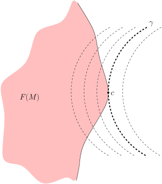
Figure 15: An outward contact point.

In the proof below we give a characterization in local coordinates.

Proposition 4.8.

Let $(M,\,\omega)$ be a connected symplectic four-manifold. Let $F:M\to\mathbb{R}^{2}$ be an almost-toric system with critical value set $\Sigma_{F}$. Let $f$ be a Morse function defined on an open neighborhood of $F(M)\subset\mathbb{R}^{2}$ such that

1. The critical set of $f$ is disjoint from $\Sigma_{F}$;

2. $f$ has no saddle points in $F(M)$;

3. the regular level sets of $f$ intersect $\Sigma_{F}$ transversally or have a non-degenerate outward contact with $F(M)$. (See definitions 4.3 and 4.3.)

Then $f\circ F:M\to\mathbb{R}$ is a Morse-Bott function with all indices and co-indices equal to 0, 2, or 3.

Proof.

Because of Theorem 4.6, we just need to prove the statement about the indices of $f$. At points of $F^{-1}(\textup{Crit}(f))$, we saw in (6) that the transversal Hessian of $f\circ F$ is just the Hessian of $f$. By assumption, $f$ has no saddle point, so its (co)index is either $0$ or $2$. We analyze the various possibilities at points of $\textup{Crit}(F)$. There are two possible rank 0 cases for an almost-toric system: elliptic-elliptic and focus-focus. At such points, the Hessian determinant is positive (see Theorem 2.3), so the index and co-index are even.

In the rank 1 case, for an almost-toric system, only transversally elliptic singularities are possible. We are interested in the case of a tangency (otherwise $f\circ F$ has no critical point). The Hessian is computed in (8) and we use below the same notations. The level set of $f$ through the tangency point is given by $f(x,y)=f(g(0,0))$. We switch to the coordinates $(\xi_{1},q)=g^{-1}(x,y)$, where the local image of $F$ is the half-space $\{q\geqslant 0\}$. Let

$$h=f\circ g-f(g(0,0)).$$

The level set of $f$ is $h(\xi_{1},q)=0$, and $h$ satisfies $\mathrm{d}_{0}h\neq 0$, $\frac{\partial h}{\partial\xi_{1}}(0,0)=0$, $\frac{\partial^{2}h}{\partial\xi_{1}^{2}}(0,0)\neq 0$ (this is the non-degeneracy condition in Definition 4.3). By the implicit function theorem, the level set $\{h=0\}$ near the origin is the graph $\{(\xi_{1},q)\mid q=\varphi(\xi_{1})\}$, where

$$\varphi^{\prime}(0)=0,\qquad\varphi^{\prime\prime}(0)=\frac{-\frac{\partial^{2}h}{\partial\xi_{1}^{2}}(0,0)}{\frac{\partial h}{\partial q_{2}}(0,0)}\;.$$

This level set has an outward contact if and only if $\varphi^{\prime\prime}(0)<0$ or, equivalently, $\frac{\partial^{2}h}{\partial\xi_{1}^{2}}(0,0)$ and $\frac{\partial h}{\partial q_{2}}(0,0)$ have the same sign. From (8) we see that the index and coindex can only be 0 or 3. ∎

4.4 Proof of Theorem 2 and Theorem 5

We conclude by proving the two theorems in the introduction. Both will rely on the following result. In the statement below, we use the stratified structure of the bifurcation set of a non-degenerate integrable system, as given by Proposition 4.3.

Proposition 4.9.

Let $(M,\,\omega)$ be a connected symplectic four-manifold. Let $F\colon M\to\mathbb{R}^{2}$ be an almost-toric system such that $F$ is proper. Denote by $\Sigma_{F}$ the bifurcation set of $F$. Assume that there exists a diffeomorphism $g\colon F(M)\to\mathbb{R}^{2}$ onto its image such that:

1. $g(F(M))$ is included in a proper convex cone $C_{\alpha,\,\beta}$ (see Figure 3).

2. $g(\Sigma_{F})$ does not have vertical tangencies (see Figure 2).

Write $g\circ F=(J,H)$. Then $J$ is a Morse-Bott function with connected level sets.

Proof.

Let $\tilde{F}:=g\circ F$. The set of critical values of $\tilde{F}$ is $\tilde{\Sigma}=g(\Sigma_{F})$. We wish to apply Proposition 4.8 to this new map $\tilde{F}$. Let $f:\mathbb{R}^{2}\to\mathbb{R}$ be the projection on the first coordinate: $f(x,y)=x$, so that $f\circ\tilde{F}=J$. Since $f$ has no critical points, it satisfies the hypotheses (i) and (ii) of Proposition 4.8. The regular levels sets of $f$ are the vertical lines, and the fact that $\tilde{\Sigma}$ has no vertical tangencies means that the regular level sets of $f$ intersect $\tilde{\Sigma}$ transversally. Thus the last hypothesis (iii) of Proposition 4.8 is fulfilled and we conclude that $J$ is a Morse-Bott function whose indices and co-indices are always different from 1.

Now, since $\tilde{F}$ is proper, the fact that $\tilde{F}(M)$ is included in a cone $C_{\alpha,\beta}$ easily implies that $f\circ\tilde{F}$ is proper. Thus, using Proposition 3.5, we conclude that $J$ has connected level sets. ∎

Proof of theorem 2.

By Proposition 4.9, we get that $J$ has connected level sets. It is enough to apply Theorem 3.7 to conclude that $\tilde{F}$ (and thus $F$) has connected fibers. ∎

Proof of theorem 5.

Using again Proposition 4.9, we conclude that $J$ is a Morse-Bott function with connected level sets. By the definition of an integrable system, $J$ cannot be constant (its differential would vanish everywhere). Thus we can apply Theorem 4.2, which yields the desired conclusion. ∎

It turns out that even in the compact case, Theorem 2 has quite a striking corollary, which we stated as Theorem 3 in the introduction.

Proof of Theorem 3.

The last two cases (a disk with two conic points and a polygon) can be transformed by a diffeomorphism as in Theorem 1 to remove vertical tangencies, and hence the theorem implies that the fibers of $F$ are connected.

For the first two cases, we follow the line of the proof of theorem 1. The use of Proposition 4.8 is still valid for the same function $f(x,y)=x$ even if now the level sets of $f$ can be tangent to $\Sigma_{F}$. Indeed one can check that here only non-degenerate outward contacts occur. Then one can bypass Proposition 4.9 and directly apply Proposition 3.5. Therefore the conclusion of the theorem still holds. ∎

5 The spherical pendulum

The goal of this section is to prove that the spherical pendulum is a non-degenerate integrable system to which our theorems apply. The configuration space is $S^{2}$.

We identify the phase space ${\rm T}^{\ast}S^{2}$ with the tangent bundle ${\rm T}S^{2}$ using the standard Riemannian metric on $S^{2}$ naturally induced by the inner product on $\mathbb{R}^{3}$. Denote the points in $\mathbb{R}^{3}$ by $\mathbf{q}$. The conjugate momenta are denoted by $\mathbf{p}$ and hence the canonical one- and two-forms are $p_{i}\mathrm{d}q^{i}$ and $\mathrm{d}q^{i}\wedge\mathrm{d}p_{i}$, respectively. The manifold ${\rm T}S^{2}$ has its own natural exact symplectic structure. It is easy to see that $\iota:{\rm T}S^{2}\hookrightarrow\mathbb{R}^{3}$ is a symplectic embedding since $\iota^{\ast}\left(p_{i}\mathrm{d}q^{i}\right)$ coincides with the canonical one-form on ${\rm T}S^{2}$. The action given by rotations about the $\mathbf{k}$-axis is given by

$$\mathbf{q}\in\mathbb{R}^{3}\mapsto\begin{bmatrix}\cos\psi&-\sin\psi&0\\ \sin\psi&\cos\psi&0\\ 0&0&1\end{bmatrix}\mathbf{q}\in\mathbb{R}^{3},\qquad\psi\in\mathbb{R}.$$

The equations of motion determined by the infinitesimal generator of the Lie algebra element $1\in\mathbb{R}$ for the lifted action to ${\rm T}\mathbb{R}^{3}=\mathbb{R}^{3}\times\mathbb{R}^{3}$ are

$$\dot{\mathbf{q}}=-\mathbf{q}\times\mathbf{k},\qquad\dot{\mathbf{p}}=-\mathbf{p}\times\mathbf{k}.$$ (9)

The $S^{1}$-invariant momentum map of this action is given by (see, e.g., [35, Theorem 12.1.4]) $J_{T\mathbb{R}^{3}}(\mathbf{q},\mathbf{p})=(\mathbf{q}\times\mathbf{p})\cdot\mathbf{k}=q^{1}p_{2}-q^{2}p_{1}$. Note that ${\rm T}S^{2}$ is invariant under the flow of (9) and thus $J:=J_{{\rm T}\mathbb{R}^{3}}|_{{\rm T}S^{2}}:{\rm T}S^{2}\rightarrow\mathbb{R}$ given for all $(\mathbf{q},\mathbf{p})\in{\rm T}S^{2}$ is the momentum map of the $S^{1}$-action on ${\rm T}S^{2}$. In particular, the equations of motion of the Hamiltonian vector field $\mathcal{H}_{J}$ on ${\rm T}S^{2}$ are (9). We also have $J({\rm T}S^{2})=\mathbb{R}$; indeed, if $\mathbf{q}=(1,0,0)$ and $\mathbf{p}=(0,p_{2},p_{3})$, then

$$J(\mathbf{q},\mathbf{p})=q^{1}p_{2}-q^{2}p_{1}=p_{2}$$

is an arbitrary element of $\mathbb{R}$. The momentum map $J$ is not proper: the sequence $(\mathbf{q}_{n},\mathbf{p}_{n}):=((0,0,1),(n,n,0))\in{\rm T}S^{2}$ does not contain any convergent subsequence and the sequence of images $J(\mathbf{q}_{n},\mathbf{p}_{n})=0$ is constant, hence convergent.

Let us describe the equations of motion. The Hamiltonian of the spherical pendulum is

$$H(\mathbf{q},\mathbf{p})=\frac{1}{2}\|\mathbf{p}\|^{2}+\mathbf{q}\cdot\mathbf{k},(\mathbf{q},\mathbf{p})\in{\rm T}S^{2},$$ (10)

where $\mathbf{i},\mathbf{j},\mathbf{k}$ is the standard orthonormal basis of $\mathbb{R}^{3}$ with $\mathbf{k}$ aligned with and pointing opposite the direction of gravity and we set all parametric constants equal to one. The equations of motion for $(\mathbf{q},\mathbf{p})\in{\rm T}S^{2}$ are given by

$$\left\{\begin{aligned} \dot{\mathbf{q}}&=\mathbf{p}-\frac{\mathbf{q}\cdot\mathbf{p}}{\|\mathbf{q}\|^{2}}\mathbf{q}=\mathbf{p}\\ \dot{\mathbf{p}}&=-\mathbf{k}-\frac{\|\mathbf{p}\|^{2}}{\|\mathbf{q}\|^{2}}\mathbf{q}+\frac{\mathbf{q}\cdot\mathbf{k}}{\|\mathbf{q}\|^{2}}\mathbf{q}+\frac{\mathbf{q}\cdot\mathbf{p}}{\|\mathbf{q}\|^{2}}\mathbf{p}=-\mathbf{k}+\left(\mathbf{q}\cdot\mathbf{k}-\|\mathbf{p}\|^{2}\right)\mathbf{q}.\end{aligned}\right.$$ (11)

Figure 16: The spherical pendulum.

Theorem 5.1.

Let $F:=(J,\,H)\colon M\to{\mathbb{R}}^{2}$ be the singular fibration associated with the spherical pendulum.

• $F$ is an integrable system.

• The singularities of $F$ are non-degenerate.

• The singularities of $F$ are of focus-focus, elliptic-elliptic, or transversally elliptic-type so, in particular, $F$ has no hyperbolic singularities. There is precisely one elliptic-elliptic singularity at $((0,0,-1),(0,0,0))$, one focus-focus singularity at $((0,0,1),(0,0,0))$, and uncountably many singularities of transversally-elliptic type.

• $H$ is proper and hence $F$ is also proper, even though $J$ is not proper.

• The critical set of $F$ and the bifurcation set of $F$ are equal and given in Figure 17: it consists of the boundary of the planar region therein depicted and the interior point which corresponds to the image of the only focus-focus point of the system; see point (3) above.

• The fibers of $F$ are connected.

• The range of $F$ is equal to planar region in Figure 17. The image under $F$ of the focus-singularity is the point $(0,\,1)$. The image under $F$ of the elliptic-elliptic singularity is the point $(0,\,-1)$.

Proof.

We prove each item separately.

(1) Integrability.

Since the Hamiltonian $H$ is $S^{1}$-invariant, the associated momentum map $J$ is conserved, i.e., $\{H,J\}=0$. To prove integrability, we need to show that $\mathrm{d}H$ and $\mathrm{d}J$ are linearly independent almost everywhere on ${\rm T}S^{2}$. Note that if $(\mathbf{q},\mathbf{p})\in{\rm T}S^{2}$, the one-forms $\mathrm{d}H(\mathbf{q},\mathbf{p})$ and $\mathrm{d}J(\mathbf{q},\mathbf{p})$ are linearly dependent precisely when the vector fields (11) and (9) are linearly dependent. Thus we need to determine all $\mathbf{q},\mathbf{p}\in\mathbb{R}^{3}$ such that there exist $a,b\in\mathbb{R}$, not both zero, satisfying $a\mathbf{p}-b\mathbf{q}\times\mathbf{k}=0$, $-a\mathbf{k}+a\left(\mathbf{q}\cdot\mathbf{k}-\|\mathbf{p}\|^{2}\right)\mathbf{q}-b\mathbf{p}\times\mathbf{k}=0$, $\|\mathbf{q}\|^{2}=1$, $\mathbf{q}\cdot\mathbf{p}=0$. A computation gives that the set of points $(\mathbf{q},\mathbf{p})\in{\rm T}S^{2}$ for which $\mathrm{d}H$ and $\mathrm{d}J$ are linearly dependent is the measure zero set:

$$\left\{((0,0,1),(0,0))\right\}\cup\left\{\left.\left(\mathbf{q},\frac{1}{\lambda}\mathbf{q}\times\mathbf{k}\right)\right|\;q^{3}=-\lambda^{2},\;(q^{1})^{2}+(q^{2})^{2}=1-\lambda^{4},\;0<|\lambda|\leqslant 1\right\}.$$ (12)

(2) Non-degeneracy.

All critical points of $F:=(J,H):{\rm T}S^{2}\rightarrow\mathbb{R}^{2}$ are non-degenerate. We prove it for rank 1 critical points. The non-degeneracy at the rank 0 critical points $((0,0,1),(0,0,0))$ and $((0,0,-1),(0,0,0))$ are similar exercices (the computation for the point $((0,0,1),(0,0,0))$ may also be found in [48]). So we consider the singularities $(\mathbf{q}_{0},\mathbf{p}_{0})$ given by $-q^{3}_{0}=\lambda^{2}$, $\mathbf{p}_{0}=\frac{1}{\lambda}\mathbf{q}_{0}\wedge{\bf k}$, where $\lambda\in(0,\,1)$ (and hence $q^{3}_{0}\in(-1,\,0)$). We have $\mathrm{d}J(\mathbf{q}_{0},\,\mathbf{p}_{0})\neq 0$ and $\mathrm{d}H(\mathbf{q}_{0},\,\mathbf{p}_{0})\neq 0$. As explained at the beginning of the section, the component $J$ is a momentum map for a Hamiltonian $S^{1}$-action. The flow of $J$ rotates about the $\mathbf{k}$ axis, so any vertical plane is transversal to the flow in the $\mathbf{q}$-coordinates. The surface $\Sigma$ obtained by intersecting the level set of $J$ with the plane $q_{2}=0$ is chosen as the symplectic transversal surface to the flow of $\mathcal{H}_{H}$. The restriction of $J(\mathbf{q},\mathbf{p})=q^{1}p_{2}-q^{2}p_{1}$ to $\Sigma$ is $J|_{\Sigma}(\mathbf{q},\mathbf{p})=q^{1}p_{2}$, so that $q^{1}p_{2}$ is constant on $\Sigma$.

We work near $(\mathbf{q}_{0},\,\mathbf{p}_{0})$, so $q^{1}\neq 0$, and hence on $\Sigma$ we have

$$p_{2}=J/q^{1},\,\,\,\,\,\,q^{3}=-\sqrt{1-(q^{1})^{2}},\,\,\,\,\,\,q^{1}p_{1}+q^{3}p_{3}=0\,\,\,\Rightarrow\,\,\,p_{3}=\frac{q^{1}p_{1}}{\sqrt{1-(q^{1})^{2}}}.$$ (13)

So $\Sigma$ may be smoothly parametrized by the coordinates $(q^{1},p_{1})$ using (13). Let us compute the Hessian of $H$ at $(\mathbf{q}_{0},\,\mathbf{p}_{0})$ in these coordinates. The Taylor expansion of $H$ at $(\mathbf{q}_{0},\,\mathbf{p}_{0})$ is

$$H=\frac{1}{2}(p_{1}^{2}+p_{2}^{2}+p_{3}^{2})+q_{3}=\frac{1}{2}\left(p_{1}^{2}+\frac{J}{(q^{1})^{2}}+\frac{(q^{1})^{2}p_{1}^{2}}{1-(q^{1})^{2}}\right)-\sqrt{1-(q^{1})^{2}}.$$

By (12) we get $(p_{1}^{0},\,p_{2}^{0},\,p_{3}^{0})=(q_{2}^{0},\,-q_{1}^{0},\,0)/\lambda$ and hence the critical point is

$$(\mathbf{q}_{0},\mathbf{p}_{0})=\left(q^{1}_{0},\,0,\,q^{3}_{0}=\sqrt{1-(q^{1}_{0})^{2}},\,0,\,p_{2}^{0}=J/q^{1}_{0},\,p_{3}^{0}=0\right).$$

To simplify notation, let us denote $s=(q^{1})^{2}\in[0,1]$; thus $(s,p_{1})$ are the smooth local coordinates near $(\mathbf{q}_{0},\mathbf{p}_{0})\simeq(s_{0},\mathbf{p}_{1}^{0})$ and the expression on the Hamiltonian is

$$H=\frac{1}{2}\left(p_{1}^{2}+\frac{J^{2}}{s}+\frac{sp_{1}^{2}}{1-s}\right)-\sqrt{1-s}=p_{1}^{2}\left(\frac{1}{2}+\frac{s}{2(1-s)}\right)+\frac{J^{2}}{2s}-\sqrt{1-s}$$ (14)

The first term in (14) is equal to

$$p_{1}^{2}\left(\frac{1}{2}+\frac{s_{0}}{2(1-s_{0})}\right)+\mathcal{O}((s-s_{0},p_{1})^{3}),$$

while the Taylor expansion of the second term $\Big{(}\frac{J^{2}}{2s}-\sqrt{1-s}\Big{)}$ with respect to $s$ is

$$\left(\frac{J^{2}}{2s_{0}}-\sqrt{1-s_{0}}\right)+(s-s_{0})\left(-\frac{J^{2}}{2s_{0}^{2}}+\frac{1}{2\sqrt{1-s_{0}}}\right)+(s-s_{0})^{2}\left(\frac{J^{2}}{s_{0}^{3}}+\frac{1}{4(1-s_{0})^{3/2}}\right)+\mathcal{O}((s-s_{0})^{3}).$$

The coefficient $\left(-\frac{J^{2}}{2s_{0}^{2}}+\frac{1}{2\sqrt{1-s_{0}}}\right)$ vanishes since $\mathrm{d}H|_{\Sigma}(\mathbf{q}_{0},\,\mathbf{p}_{0})=0$, so the Hessian $\operatorname{Hess}(H|_{\Sigma})(s,p_{1})$ of $H_{\Sigma}$ is of the form $Ap_{1}^{2}+B(s-s_{0})^{2}$, where $A>0$ and $B>0$, which is non-degenerate, as we wanted to show.

(3) The nature of the singularities of $F$.

The statement in the theorem follows from the computations in (2). The equilibrium $((0,0,1),(0,0,0))$ is of focus-focus type and the equilibrium $((0,0,-1),(0,0,0))$ is of elliptic-elliptic type. The other critical points are of transversally-elliptic type.

(4) $H$ and $F$ are proper maps.

The properness of $H$ follows directly from the defining formula (10); indeed, on ${\rm T}S^{2}$, the map $(\mathbf{q},\mathbf{p})\mapsto\mathbf{q}\cdot\mathbf{k}$ takes values in a compact set, hence if $K\subset\mathbb{R}$ is compact, there is a compact set $K^{\prime}\subset\mathbb{R}$ such that $H^{-1}(K)$ is closed in $\{(\mathbf{q},\mathbf{p})\mid\|\mathbf{p}\|^{2}\in K^{\prime}\}$ and hence is compact. Thus $H$ is proper.

Then for any compact set $C\subset\mathbb{R}^{2}$, $F^{-1}(C)\subset H^{-1}(\operatorname{pr}_{2}(C))$ is compact, thus $F$ is proper as well. ($\operatorname{pr}_{2}:\mathbb{R}^{2}\rightarrow\mathbb{R}$ is the projection on the second factor).

On the other hand it is clear that the level sets of $J$ are unbounded, so $J$ cannot be proper.

(5) Critical and bifurcation sets.

The critical set is the image of (12) by the map $(J,\,H):{\rm T}S^{2}\rightarrow\mathbb{R}^{2}$. We have $J((0,0,\pm 1),(0,0,0))=0$, $H((0,0,\pm 1),(0,0,0))=\pm 1$. In addition,

$$\left\{\begin{aligned} J\left(\mathbf{q},\frac{1}{\lambda}\mathbf{q}\times\mathbf{k}\right)&=-\frac{1}{\lambda}\left(\left(q^{1}\right)^{2}+\left(q^{2}\right)^{2}\right)=\frac{\lambda^{4}-1}{\lambda}=:j(\lambda)\\ H\left(\mathbf{q},\frac{1}{\lambda}\mathbf{q}\times\mathbf{k}\right)&=\frac{1}{2\lambda^{2}}\left(\left(q^{1}\right)^{2}+\left(q^{2}\right)^{2}\right)+q^{3}=\frac{1-\lambda^{4}}{2\lambda^{2}}-\lambda^{2}=\frac{1-3\lambda^{4}}{2\lambda^{2}}=:h(\lambda)\end{aligned}\right.$$

for $0<|\lambda|<1$ which is a parametric curve with two branches. We can give an Cartesian equation for this curve. An analysis of $h(\lambda)$ for $0<|\lambda|\leqslant 1$ shows that $h(\lambda)\geqslant-1$. Eliminating $\lambda$ yields the two branches

$$j(h)=\pm\frac{2}{9}\left(3-h^{2}+h\sqrt{h^{2}+3}\right)\sqrt{h+\sqrt{h^{2}+3}},$$

for $h\geqslant-1$. The critical set is given in Figure 17. The graph intersects the horizontal momentum axis at $j=\pm 2\sqrt[4]{3}/3$ and at the lower tip $(j,h)=(0,-1)$ the graph is not smooth.

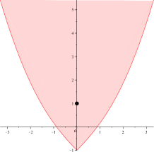
Figure 17: Image the momentum-energy map for the spherical pendulum. The bifurcation set $\Sigma_{F}$ is its boundary plus the focus-focus value $(0,1)$.

Since $F$ is proper, the bifurcation set equals the set of critical values of the system, see Figure 17.

(6) The fibers of $F$ are connected.

This follows from item (5) and Theorem 3.7.

Compare this with the result [15, page 160, Table 3.2] whose proof is quite difficult (however, it also gives the description of the fibers of $F$).

(7) Range of the momentum-energy set.

The range of the momentum-energy set is the epigraph of the critical set shown in Figure 17: this follows from item (iv) in Theorem 2.6.

∎

6 Final remarks

Real solutions sets

To motivate further our connectivity results (Theorem 1 and Theorem 2), consider on the real plane with coordinates $(x,\,y)$ the following question: is the solution set of the polynomial equation $\,(x^{2}-1)\,y^{2}\,=\,0\,$ connected? Surely the answer is yes, since the solution set consists of two parallel vertical lines and an intersecting horizontal line: $\{x=-1\}\cup\{x=1\}\cup\{y=0\}$. One can modify this equation slightly to consider the equation $\,(x^{2}-1)\,(y^{2}+\epsilon^{2})\,=\,0\,$, $\epsilon\neq 0$. In this case the solution set $\{x=-1\}\cup\{x=1\}$ is disconnected, so a small perturbation of the original equation leads to a disconnected solution set (see Figure 18). As is well known in real algebraic geometry, the connectivity question is not stable under small perturbations, so any technique to detect connectivity must be sensitive to this issue.

Although in all of these examples the answers are immediate, one can easily consider equations for which answering this connectivity question is a serious challenge.

Figure 18: Solution sets of the polynomial equations $(x^{2}-1)y^{2}=0$ and $(x^{2}-1)(y^{2}+\epsilon^{2})=0$, $\epsilon\neq 0$.

This question may be put in a general framework in two alternative, equivalent, ways. Consider functions $f_{1},\,\,\ldots,\,\,f_{n}\,\,\colon\,\,M\subseteq\mathbb{R}^{m}\to\mathbb{R}$ and constants $\lambda_{1},\,\ldots,\,\lambda_{n}\in\mathbb{R}$, where $M$ is a connected manifold. Is the solution set $\mathcal{S}\subset\mathbb{R}^{m}$ of

$$\left\{\begin{array}[]{rl}f_{1}\,(x_{1},\,\ldots,\,x_{m})&\,\,=\,\,\,\,\lambda_{1}\\ \textup{\,}\vdots\\ f_{n}\,(x_{1},\,\ldots,\,x_{m})&\,\,=\,\,\,\,\lambda_{n}\end{array}\right.$$ (18)

a connected subset of $M$? Equivalently, are the fibers $F^{-1}(\lambda_{1},\,\ldots,\,\lambda_{n})$ of the map $F\colon M\,\subseteq\,\mathbb{R}^{m}\longrightarrow\mathbb{R}^{n}$ defined by

$$F(x_{1},\,\ldots,\,x_{m})\,\,:=\,\,(f_{1}(x_{1},\,\ldots,\,x_{m}),\,\,\,\ldots\,\,\,,\,\,\,f_{n}(x_{1},\,\ldots,\,x_{m}))$$

connected? If $F$ is a scalar valued function (i.e., if there is only one equation in the system) a well-known general method exists to answer it when $F$ is smooth, namely, Morse-Bott theory. We saw in Proposition 3.5 that if $M$ is a connected smooth manifold and $f:M\rightarrow\mathbb{R}$ is a proper Morse-Bott function whose indices and co-indices are always different from 1, then the level sets of $f$ are connected.

In order to motivate the idea of this result further consider the following example: the height function defined on a $2$-sphere, and the same height function defined on a $2$-sphere in which the North Pole is pushed down creating two additional maximum points and a saddle point, as in Figure 19. When the height function is considered on the $2$-sphere, it has connected fibers. On the other hand, when it is considered on the right figure, many of its fibers are disconnected. The “essential” difference between these two examples is that in the second case the function has a saddle point, while in the first case it doesn’t. A saddle point has index 1.

Figure 19: Height function.

Next, let us look at an example of a vector valued function. Consider $M=S^{2}\times{\mathbb{R}}^{2}\subset\mathbb{R}^{5}$ with coordinates $(x,\,y,\,z,\,u,\,v)$. Is the solution set $\mathcal{S}$ of

$$\left\{\begin{array}[]{rl}2u^{2}+2v^{2}+z&\,\,=\,\,\,\,1\\ ux+vy&\,\,=\,\,\,\,0\end{array}\right.$$

connected? In other words, is the set $F^{-1}(1,\,0)$ connected, where $F\colon S^{2}\times{\mathbb{R}}^{2}\to\mathbb{R}^{2}$ defined by

$$F(x,y,z,u,v):=(2u^{2}+2v^{2}+z,\,\,ux+vy)?$$

One is tempted to again use Morse-Bott theory to check this connectivity, but Morse-Bott theory for which function? The first goal of the present paper was to give a method to answer connectivity questions of this type in the case $F$ is an integrable system. In the paper we introduced a method to construct Morse-Bott functions which, from the point of view of symplectic geometry, behave well near singularities. We saw how the behavior of an integrable system near the singularities has a strong effect on the global properties of the system.

The fibers of $F\colon S^{2}\times{\mathbb{R}}^{2}\to\mathbb{R}^{2}$ are, by the Theorem 2, connected, because its image can be easily seen to be given by Example 12. The question answered by Theorem 2 is probably the most basic topological question to ask about a solution set (except for its non-emptyness).

Semiclassical quantization

Semiclassical quantization is a strong motivation for undergoing the systematic study of integrable systems in this paper. Consider the quantum version of the connectivity problem. The functions $f_{1},\dots,f_{n}$ are replaced by “quantum observables”, i.e., self-adjoint operators $\hat{f}_{1},\dots,\hat{f}_{n}$ on a Hilbert space $\mathcal{H}$, and the system of fiber equations (18) is replaced by the system

$$\left\{\begin{aligned} \hat{f}_{1}\psi&=\lambda_{1}\psi\\ \vdots&\\ \hat{f}_{n}\psi&=\lambda_{n}\psi\end{aligned}\right.\qquad\psi\in\mathcal{H}.$$

So $\lambda_{i}$ should be an eigenvalue for $\hat{f}_{i}$ and the eigenvector $\psi$ should be the same for all $i=1,\dots,n$. There is a chance to solve this when the operators $\hat{f}_{i}$ pairwise commute. This is the quantum analogue of the Poisson commutation property for the integrable system given by $f_{1},\dots,f_{n}$.

In the last thirty years, semiclassical analysis has pushed this idea quite far. It is known that to any regular Liouville torus of the classical integrable system, one can associate a quasimode for the quantum system, leading to approximate eigenvalues [14, 32]. Thus, the study of bifurcation sets (described in Theorem 4 and Theorem 5) is fundamental for a good understanding of the quantum spectrum. More recently, quasimodes associated to singular fibers have been constructed; see [48] and the references therein. In some case, it can be shown that the quantum spectrum completely determines the classical system, see Zelditch [52].

When the system has symmetries, the quantum spectrum typically exhibits degenerate (or almost degenerate) eigenvalues. In the setting of integrable systems, this is revealed by the non-connectedness of some fibers. Thus, connectivity results are of primary importance from the quantum perspective. They predict almost degenerate (or clusters of) eigenvalues. For instance, in the inverse spectral result of [48], detecting the number of connected components was the key point (and the most subtle) of the analysis.

Singular Lagrangian fibrations

Theorem 1 and Theorem 2 may have applications to mirror symmetry and symplectic topology. An integrable system without hyperbolic singularities gives rise to a toric fibration with singularities. The base space is endowed with a singular integral affine structure. Remarkably, these singular affine structures are of key importance in various parts of symplectic topology, mirror symmetry, and algebraic geometry; for example they play a central role in the work of Kontsevich and Soibelman [30]. These singular affine structures have been studied in the context of integrable systems (in particular by Nguyên Tiên Zung [53]), but also became a central concept in the works by Symington [46] and Symington-Leung [34] in the context of symplectic geometry and topology, and by Gross-Siebert, Castaño-Bernard, Castaño-Bernard-Matessi [25, 26, 24, 23, 10, 11, 12], among others, in the context of mirror symmetry and algebraic geometry. Fiber connectivity is (usually) assumed in theorems about Lagrangian fibrations, so the theorem above gives a method to test whether a given result in that context applies to a Lagrangian fibration arising from an integrable system. See also Eliashberg-Polterovich [18, page 3] for relevant examples in the theory of symplectic quasi-states.

Toric and semitoric systems

Non-degenerate integrable systems without hyperbolic singularities are prominent in the literature, both in mathematics and in physics; see for instance [5, 46, 49]. They are usually called almost-toric systems, although the choice of name is somewhat misleading as they may not have any periodicity from a circle or torus action; on the other hand, these systems retain some properties of toric systems, at least in the compact case. The most well studied case of almost-toric system is that of toric systems coming from a Hamiltonian torus actions.

A proof of Theorem 2 for the so called “semitoric” systems was given by the third author in [49] using the theory of Hamiltonian circle actions. Semitoric systems are integrable systems on four-manifolds which have no hyperbolic singularities and for which one component of the system generates a proper periodic flow. The proof in [49] uses in an essential way the periodicity assumption and it cannot be extended, as far as we know, to deal with the general systems treated in Theorem 2. A classification of semitoric systems in terms of five symplectic invariants was given by the first and third authors in [38, 40].

Álvaro Pelayo
School of Mathematics
Institute for Advanced Study
Einstein Drive
Princeton, NJ 08540 USA.

and

Washington University, Mathematics Department
One Brookings Drive, Campus Box 1146
St Louis, MO 63130-4899, USA.
E-mail: apelayo@math.wustl.edu

Tudor S. Ratiu
Section de Mathématiques and Bernoulli Center
Station 8
Ecole Polytechnique Fédérale de Lausanne
CH-1015 Lausanne, Switzerland
E-mail: tudor.ratiu@epfl.ch

Vũ Ngọc San
Institut Universitaire de France

and

Institut de Recherches Mathématiques de Rennes
Université de Rennes 1
Campus de Beaulieu
F-35042 Rennes cedex, France
E-mail: san.vu-ngoc@univ-rennes1.fr

References

- [1] Abraham, R. and Marsden, J.E.: Foundation of Mechanics, Second edition, revised and enlarged. With the assistance of Tudor Ratiu and Richard Cushman. Benjamin/Cummings Publishing Co., Inc., Advanced Book Program, Reading, Mass., 1978.
- [2] Assémat, E., Efstathiou, K., Joyeux, M., and Sugny, D.: Fractional bidromy in the vibrational spectrum of HOCl. Phys. Rev. Letters, 104 (113002) (2010), 1–4.
- [3] Atiyah, M.: Convexity and commuting Hamiltonians, Bull. London Math. Soc., 14 (1982), 1–15.
- [4] Bott, R. Morse theory indomitable. Inst. Hautes Études Sci. Publ. Math. No. 68 (1988).
- [5] Babelon, O., Cantini, L., Douçcot, B.: A semi-classical study of the Jaynes-Cummings model, J. Stat. Mech. Theory Exp., 7 (2009), P06013.
- [6] Babelon, O. and Douçot, B.: Classical Bethe Ansatz and Normal Forms in the Jaynes-Cummings Model, arXiv:1106.3274.
- [7] Banyaga, A.; Hurtubise, D. E. A proof of the Morse-Bott lemma. Expo. Math. 22 (2004), no. 4, 365–373.
- [8] Bolsinov, A. V. and Fomenko, A. T.: Integrable Hamiltonian Systems; Geometry, Topology, Classification, Chapman & Hall, 2004.
- [9] Bourbaki, N.: General Topology, Part I, Hermann, Paris, Addison-Wesley Publishing Co, Reading, 1966.
- [10] Castaño-Bernard, R.: Symplectic invariants of some families of Lagrangian -fibrations, J. Symplectic Geometry, 2(3) (2004), 279–308.
- [11] Castaño-Bernard, R. and Matessi, D.: Some piece-wise smooth Lagrangian fibrations, Rend. Semin. Mat. Univ. Politec. Torino, 63(3) (2005), 223–253.
- [12] Castaño-Bernard, R. and Matessi, D.: Lagrangian -torus fibrations, J. Diff. Geometry, 81 (2009), 483–573.
- [13] Child, M. S., Weston, T., and Tennyson, J.: Quantum monodromy in the spectrum of and other systems: new insight into the level structure of quasi-linear molecules, Mol. Phys., 96(3) (1999), 371–379.
- [14] Colin de Verdiére, Y.: Quasi-modes sur les variétés riemanniennes, Invent. Math., 43(1) (1977), 15-Ð52.
- [15] Cushman, R.H. and Bates, L.M.: Global Aspects of Classical Integrable Systems, Birkhäuser Verlag, Basel, 1997.
- [16] Delzant T.: Hamiltoniens périodiques et image convexe de l’application moment, Bull. Soc. Math. France, 116 (1988), 315–339.
- [17] Duistermaat, J.J. and Pelayo, Á.: Reduced phase space and toric variety coordinatizations of Delzant spaces, Math. Proc. Cambridge Philos. Soc., 146 (2009), 695–718.
- [18] Eliashberg, Y. and Polterovich, L.: Symplectic quasi-states on the quadric surface and Lagrangian submanifolds, arXiv:1006.2501.
- [19] Eliasson, L.H.: Hamiltonian Systems with Poisson Commuting Integrals, Ph.D. Thesis, University of Stockholm, 1984.
- [20] Eliasson, L.H.: Normal forms for Hamiltonian systems with Poisson commuting integrals – elliptic case. Comment. Math. Helv., 65 (1990), 4–35.
- [21] Fitch, N. J., Weidner, C. A., Parazzoli, L. P., Dullin, H. R., and Lewandowski, H. J.: Experimental demonstration of classical hamiltonian monodromy in the 1:1:2 resonant elastic pendulum, Phys. Rev. Lett., 103 (2009), 034301.
- [22] Fomenko, A. T. The topology of surfaces of constant energy of integrable Hamiltonian systems and obstructions to integrability. (Russian) Izv. Akad. Nauk SSSR Ser. Mat. 50 (1986), no. 6, 1276–1307, 1344.
- [23] Gross, M. and Siebert, B.: Affine manifolds, log structures, and mirror symmetry, Turkish J. Math., 27(1) (2003), 33–60.
- [24] Gross, M. and Siebert, B.: Mirror symmetry via logarithmic degeneration data I, J. Diff. Geom., 72(2) (2006), 169–338.
- [25] Gross, M. and Siebert, B.: Mirror symmetry via logarithmic degeneration data II, J. of Alg. Geom., 19(4) (2010), 679–780.
- [26] Gross, M. and Siebert, B.: From real affine geometry to complex geometry, arXiv:math/0703822.
- [27] Guillemin, V. and Sjamaar, R.: Convexity Properties of Hamiltonian Group Actions, CRM Monograph Series, 26, Amer. Math. Soc., Providence RI, 2005.
- [28] Guillemin, V. and Sternberg, S.: Convexity properties of the moment mapping, Invent. Math., 67 (1982), 491–513.
- [29] Kirwan, F.: Convexity properties of the moment mapping III. Invent. Math., 77 (1984), 547–552.
- [30] Kontsevich, M. and Soibelman, Y.: Affine structures and non-Archimedean analytic spaces, The Unity of Mathematics, Progress in Mathematics, 244, 321–385, Birkhäuser Boston, MA, 2006.
- [31] Kostant, B.: On convexity, the Weyl group and the Iwasawa decomposition, Ann. Sci. École Norm. Sup., 6 (1973), 413–455.
- [32] Lazutkin, V. F.: KAM Theory and Semiclassical Approximations to Eigenfunctions. With an addendum by A. I. Shnirelman. Ergebnisse der Mathematik und ihrer Grenzgebiete (3), 24. Springer-Verlag, Berlin, 1993.
- [33] Lerman, E., Meinrenken, E., Tolman, S., and Woodward, C.: Non-abelian convexity by symplectic cuts, Topology, 37 (1998), 245–259.
- [34] Leung, N. C. and Symington, M.: Almost toric symplectic four-manifolds, J. Symplectic Geom., 8 (2010), 143–187.
- [35] Marsden, J. E., and Ratiu, T. S.: Introduction to Mechanics and Symmetry, Texts in Applied Mathematics, 17, second edition, second printing, Springer-Verlag, New York, 2003.
- [36] McDuff, D. and Salamon, D.: Introduction to Symplectic Topology, Oxford University Press 1994.
- [37] Milnor, J.: Morse Theory, Ann. of Math. Studies, Princeton Univ. Press, 1963.
- [38] Pelayo, Á. and Vũ Ngọc, S.: Semitoric integrable systems on symplectic -manifolds, Invent. Math., 177 (2009), 571–597.
- [39] Pelayo, Á. and Vũ Ngọc, S.: Constructing integrable systems of semitoric type, Acta Math., 206 (2011), 93–125.
- [40] Pelayo, Á. and Vũ Ngọc, S.: Symplectic theory of completely integrable Hamiltonian systems, Bull. Amer. Math. Soc., 48 (2011), 409–455.
- [41] Pelayo, Á. and Vũ Ngọc, S.: Hamiltonian dynamics and spectral theory for spin-oscillators, Com. Math. Phys., in press.
- [42] Prato, E., Convexity properties of the moment map for certain non-compact manifolds, Comm. Anal. Geom., 2(2) (1994), 267–278.
- [43] Sadovskií, D. A. and Zhilinskií, B.: Counting levels within vibrational polyads, J. Chem. Phys., 103(24) (1995), 10520–10536.
- [44] Sjamaar, R.: Convexity properties of the moment mapping re-examined, Adv. Math., 138(1) (1998), 46–91.
- [45] Smith, I.: Torus fibrations on symplectic four-manifolds, Turkish J. Math., 25 (2001)(1), 69–95.
- [46] Symington, M.: Four dimensions from two in symplectic topology, Topology and Geometry of Manifolds (Athens, GA, 2001), Proc. Sympos. Pure Math., 71, 153–208, Amer. Math. Soc., Providence, RI, 2003.
- [47] Vey, J.: Sur certains systèmes dynamiques séparables. Amer. J. Math., 100:591–614, 1978.
- [48] Vũ Ngọc, S.: Systèmes intégrables semi-classiques : du local au global, Panorama et Synthèses, Soc. Math. France, 22, 2006.
- [49] Vũ Ngọc, S.: Moment polytopes for symplectic manifolds with monodromy, Adv. Math., 208(2) (2007), 909–934.
- [50] Vũ Ngọc, S. and Wacheux, C.: Smooth normal forms for integrable Hamiltonian systems near a focus-focus singularity, arXiv:1103.3282.
- [51] Williamson, J.: On the algebraic problem concerning the normal forms of linear dynamical systems, Amer. J. Math., 58(1) (1936), 141–163.
- [52] Zelditch, S. The inverse spectral problem for surfaces of revolution. J. Differential Geom. 49 (1998) 207–264.
- [53] Nguyên Tiên Zung: Symplectic topology of integrable hamiltonian systems, I: Arnold-Liouville with singularities, Compositio Math., 101 (1996), 179–215.