Hyperon forward spin polarizabilty $\gamma_{0}$

Abstract

We present the results of a systematic leading order calculation of hyperon Compton scattering and extract the forward spin polarizability—$\gamma_{0}$—of hyperons within the framework of SU(3) heavy baryon chiral perturbation theory (HBChPT). The results obtained for $\gamma_{0}$ in the case of nucleons agree with that of the known results of SU(2) HBChPT when kaon loops are not considered.

I Introduction

Compton scattering is a source of valuable information about baryons since it offers access to some of the more subtle aspects of baryon structure such as polarizabilities AMB60 -BWF02 , which parameterize the response of the target to an external quasi-static electromagnetic field. For the case of unpolarized nucleons the spin-independent (SI) Compton amplitude is given by

$$\epsilon^{\mu}_{1}\,{\cal M}_{\mu\nu}^{\rm SI}\,\epsilon^{\nu}_{2}=\vec{\epsilon}\cdot\vec{\epsilon}^{\,*}\biggl{(}-\frac{Q^{2}_{N}}{m_{N}}+4\pi\alpha_{N}\,\omega\omega^{{}^{\prime}}\biggr{)}+4\pi\beta_{N}\ (\vec{\epsilon}\times\vec{q})\cdot(\vec{\epsilon}^{\,*}\times\vec{q}^{\,{}^{\prime}})\ +\ {\cal O}(\omega^{4})$$ (1)

where $N=p,n$; $Q_{N}$, $m_{N}$ represent the nucleon charge and mass, while $\epsilon_{\mu}=(0,\vec{\epsilon})$, $\epsilon^{\,*}_{\mu}=(0,\vec{\epsilon}^{\,*})$ and $q_{\mu}=(\omega,\vec{q})$, $q_{\mu}^{{}^{\prime}}=(\omega^{{}^{\prime}},\vec{q}^{\,{}^{\prime}})$ specify the polarization vectors and four-momenta of the initial and final photons, respectively. At this order the Compton amplitude is defined in terms of two polarizabilities—electric ($\alpha_{N}$) and magnetic ($\beta_{N}$), which measure the response of the nucleon to applied quasi-static electric and magnetic fields. By measurement of the differential cross section one can extract $\alpha_{N}$ and $\beta_{N}$ provided the energy is large enough such that the second and third term in Eq. (1) contribute significantly with respect to the leading Thomson contribution, but is not so large that higher order effects become significant. This extraction has been achieved in the energy range $50$ MeV $<\omega<100$ MeV—for a recent review see e.g. Refs. DD03 ; MS05 ; PDV11 . According to the Particle Data Group PDG current experimental numbers for $\alpha_{N}$ and $\beta_{N}$ are:

$$\alpha_{p}=(12.0\pm 0.6)\times 10^{-4}\ {\rm fm}^{3}\,,\quad\beta_{p}=(1.9\pm 0.5)\times 10^{-4}\ {\rm fm}^{3}\,,$$

$$\alpha_{n}=(11.6\pm 1.5)\times 10^{-4}\ {\rm fm}^{3}\,,\quad\beta_{n}=(3.7\pm 2.0)\times 10^{-4}\ {\rm fm}^{3}\,.$$ (2)

The nucleon polarizabilities have been studied via a number of theoretical approaches based on dispersion relations WP74 ; IG78 ; AIL81 ; AIL97 ; DD99 ; BP07 ; BRH94 , phenomenological Lagrangians VP95 ; OS96 ; TF99 ; SK01 ; KR01 , constituent quark models SC92 ; HL95 ; TUB05 , chiral-soliton type of models MC87 ; NNS89 ; SS92 ; WB93 ; NNS96 and lattice QCD using the external electromagnetic field method in quenched FXL06 ; WD06 and unquenched approximation ME07 . Additional insights into the polarizabilities have come from chiral perturbation theory (ChPT), an effective theory of the low-energy strong interaction SW79 ; JG84 , specifically from heavy baryon chiral perturbation theory (HBChPT) which is an extension of ChPT that includes the nucleon EJ91 ; EJ92 . The first such calculations of nucleon polarizabilities within ChPT were carried out in BER91 ; BER92ONE . However, HBChPT has an important deficiency in that the chiral perturbative series fails to converge in part of the low energy region. The problem is generated by a set of higher order graphs involving insertions in nucleon lines. It has been shown that infrared singularities of the various one loop graphs occurring in the chiral perturbation series can be extracted in a relativistically invariant fashion. This procedure is known as infrared dimensional regularization (IDR) TB99 . The IDR respects the constraints of chiral symmetry as expressed through the chiral Ward identities. The manifestly Lorentz-invariant form of baryon chiral perturbation theory (BChPT) with the IDR prescription has been successfully applied to calculate $\alpha_{N}$ and $\beta_{N}$ and the results for these polarizabilities differ substantially from the corresponding HBChPT numbers VL09 ; VL10 . In addition, HBChPT has been employed to analyze virtual Compton scattering processes since, as an effective field theory, it satisfies the structures of gauge invariance, Lorentz invariance and crossing symmetry DD98 . New predictions for generalized polarizabilities have been made using HBChPT at $O(p^{4})$ (NLO) TRH097 ; TRHT98 ; TRH00 and, using ChPT, Compton scattering from the deuteron has been computed to order $O(p^{4})$ SRB005 . However, the situation with regard to scattering from polarized targets is less satisfactory, in part because few direct measurements of polarized Compton scattering have been attempted.

The spin-dependent (SD) piece of the forward scattering amplitude for real photons of energy $\omega$ and momentum $q$ is BER95 ; ACH62 ; TRH98 ; BRH98 ; SRB05 ,

$$\epsilon^{\mu}_{1}\,{\cal M}_{\mu\nu}^{\rm SD}\,\epsilon^{\nu}_{2}=ie^{2}\,\omega\,W^{(1)}(\omega)\ \vec{\sigma}\cdot(\vec{\epsilon}\times\vec{\epsilon}^{\,*})+\ldots$$ (3)

From the theoretical perspective there is particular interest in the low energy limit of the amplitude:

$$e^{2}W^{(1)}(\omega)=4\,\pi\,(f_{2}(0)+\omega^{2}\,\gamma_{0}^{N})+\ldots$$ (4)

where $\gamma_{0}$ is the forward spin polarizability, which is related to the photo-absorption cross sections for parallel $(\sigma_{+})$ and antiparallel $(\sigma_{-})$ photon and target helicities via

$$\gamma_{0}^{N}=\frac{1}{4\pi^{2}}\,\int\limits_{W}^{\infty}\frac{ds}{s^{3}}\,\Big{[}\sigma_{-}(s)-\sigma_{+}(s)\Big{]}\,,$$ (5)

where $W=M_{\pi}+M_{\pi}^{2}/(2m_{N})$ is the threshold energy for an associated neutral pion in the intermediate state. The Low-Gell-Mann-Goldberger low-energy theorem states that,

$$f_{2}(0)=-\,\frac{\alpha\,\kappa_{N}^{2}}{2\,m^{2}_{N}}\,,$$ (6)

where $\alpha=e^{2}/(4\pi)=1/137.036$ is the fine-structure constant, $\kappa_{N}$ is the nucleon anomalous magnetic moment FLOW54 .

The forward spin polarizability $\gamma_{0}^{N}$ has been calculated to $O(p^{3})$ (LO) BER92 in the framework of HBChPT yielding, at lowest order in the chiral expansion,

$$\gamma_{0}^{N}=\frac{\alpha\,g^{2}_{A}}{24\,\pi^{2}\,F^{2}\,M_{\pi}^{2}}=4.54\times 10^{-4}\ {\rm fm}^{4}$$ (7)

both for protons and neutrons, where the entire contribution comes from $\pi N$ loops. (Hereafter we shall use units of $10^{-4}\,{\rm fm}^{4}$ for the spin polarizability). This LO calculation of spin polarizability is a prediction, since any low energy constants associated with the polarizability enter only at next to leading order (NLO). At LO the polarizability is given entirely by the loop contribution in terms of well known parameters such as nucleon and pion masses and the pion-nucleon coupling constant $(g_{\pi NN})$. The effect of including the $\Delta(1236)$ enters in counterterms at fifth order in standard HBChPT, and has been estimated to be so large as to change the sign. The forward nucleon spin polarizability $\gamma_{0}$ has been computed in an extension of HBChPT with an explicit $\Delta$ in TRH98 .

This calculation has also been carried out to NLO in the framework of HBChPT KBV2000 ; XJ2000 ; GCG2000 ; MCB01 . The contribution to $\gamma_{0}^{N}$ up to and including NLO contributions is found to be $\gamma_{0}^{p/n}=4.5-(6.9\pm 1.5)$—the NLO contributions are large. The corresponding relativistic chiral one loop calculation of the forward spin polarizability was carried out by Bernard et al. BER92 and the computed value of $\gamma_{0}^{N}$ was found to be smaller than the LO result of HBChPT. The generalized $\gamma_{0}^{N}$ has been calculated in the Lorentz invariant formulation of BChPT to NLO which demonstrates a large NNLO contribution BER03 ; CWK06 . In BER03 the quoted values are $\gamma_{0}^{p}=4.64$ and $\gamma_{0}^{n}=1.82$; hence the chiral expansion does not seem to converge, which is attributed to the Born terms. Also, as has been shown in Ref. BER03 , inclusion of the Born terms up to fourth order is not sufficient to obtain convergence and thus a complete fifth order calculation seems mandatory. However, when only the first two terms of the chiral expansion are considered $(O(\mu^{-1}))$ the results reproduce the NLO HBCHPT results. Electroproduction data have been used to extract $\gamma_{0}^{N}$ using the sum rule given above. In particular, in Ref. AMS94 the values $\gamma^{p}_{0}=-1.3$ and $\gamma^{n}_{0}=-0.4$ were found, while the analysis of Ref. DD98one gives a smaller absolute values with $\gamma^{p}_{0}=-0.6$ and $\gamma^{n}_{0}=+0.0$ based on the HDT parametrization. The latest numerical results of Schumacher SCH2011 ; SCH2009 based on the photo production cross section are $\gamma^{p}_{0}=-0.58\pm 0.20$ and $\gamma^{n}_{0}=-0.38\pm 0.22$. The most recent results are $\gamma^{p}_{0}=-0.90\pm 0.08\pm 0.11$ PAS2010 . Other results based on different photomeson analyses are $\gamma^{p}_{0}=-0.67$ (HDT), -0.65 (MAID), -0.86 (SAID) and -0.76 (DMT). Hence it is safe to say that, although considerable progress has been made in understanding $\gamma_{0}$ for the nucleon, the results obtained from BCHPT/HBCHPT are far from the numerical results obtained from the electroproduction data. While a rather large amount of work has been devoted, both theoretically and experimentally, to the study of the nucleon polarizabilities, very little is known about hyperon polarizabilities. However, with the advent of hyperon beams at FNAL and CERN, the experimental situation is likely to change, and this possibility has triggered a number of theoretical investigations. Already, predictions for electric and magnetic polarizabilities have been made for low-lying octet baryons in the framework of LO HBChPT BER92TWO , and in the context of several other models, yielding a broad spectrum of predictions PET81 ; LIP92 ; GOB96 ; NIS98 ; TAN2000 ; AAL11 . At present, no experimental data is available for the forward spin polarizabilty of the hyperons and no theoretical calculations have been published. Motivated by this situation, in the present work we extend the analysis of SU(2) HBChPT to the SU(3) version in order to compute $\gamma_{0}$ for hyperons. This could serve as a test of low-energy structure of QCD in the three flavor sector. However, there is also a need to compute the spin polarizabilities in the framework of BChPT with the IDR prescription.

The paper is organized as follows. Section II contains an overview of the SU(3) version of HBChPT relevant for the calculation of the hyperon forward spin polarizabilities $\gamma_{0}$. The relevant Feynman rules for the case of the $\Sigma^{+}$ polarizability are listed in Appendix A (see Fig.1), and the required loop integrals are listed in Appendix B. The explicit expressions for $\Sigma^{+}{\pi}^{+}(K^{+})$ loops in terms of loop integrals are listed in Appendix C. In Section III we give the explicit results for the hyperon spin polarizabilities $\gamma_{0}$ and discuss the corresponding numerical results. Brief conclusions are given in Section IV.

II Effective Lagrangian

The lowest-order SU(3) HBChPT Lagrangian involving the octet of pseudoscalar mesons $\phi$

$$\phi={\sqrt{2}}\left(\begin{array}[]{ccc}\frac{1}{\sqrt{2}}\pi^{0}+\frac{1}{\sqrt{6}}\eta&\pi^{+}&K^{+}\\ \pi^{-}&-\frac{1}{\sqrt{2}}\pi^{0}+\frac{1}{\sqrt{6}}\eta&K^{0}\\ K^{-}&\bar{K}^{0}&-\frac{2}{\sqrt{6}}\eta\\ \end{array}\right)$$ (11)

and the baryon octet $B$

$$B=\left(\begin{array}[]{ccc}\frac{1}{\sqrt{2}}\Sigma^{0}+\frac{1}{\sqrt{6}}\Lambda&\Sigma^{+}&p\\ \Sigma^{-}&-\frac{1}{\sqrt{2}}\Sigma^{0}+\frac{1}{\sqrt{6}}\Lambda&n\\ \Xi^{-}&\Xi^{0}&-\frac{2}{\sqrt{6}}\Lambda\\ \end{array}\right)$$ (15)

consists of two basic pieces: the lowest-order chiral effective meson Lagrangian ${\cal L}^{(2)}_{\phi\phi}$ SW79 ; JG84

$${\cal L}_{\phi\phi}^{(2)} = \frac{F^{2}}{4}\,\langle\nabla_{\mu}U\,\nabla^{\mu}U^{\dagger}\,+\,\chi_{+}\rangle$$ (16)

and the lowest-order meson-baryon Lagrangian ${\cal L}^{(1)\ {\rm HHChPT}}$ EJ91 ; EJ92 ; BER95 :

$${\cal L}^{(1)\ {\rm HBChPT}}_{\phi\,B}=\langle\bar{B}(i\,v\cdot D)B\rangle+\frac{D}{F_{0}}\,\langle\bar{B}\,S^{\mu}\{u_{\mu},B\}\rangle+\frac{F}{F_{0}}\,\langle\bar{B}\,S^{\mu}[u_{\mu},B]\rangle\,.$$ (17)

where the superscript $(i)$ attached to the above Lagrangians denotes their low-energy dimension and the symbols $\langle\,\,\rangle$, $[\,\,]$, $\{\,\,\}$ denote the trace over flavor matrices, commutator and anticommutator, respectively. We use the following notations: $U=u^{2}=\exp(i\phi/F_{0})$, where $F_{0}$ is the octet decay constant (in our calculations we use $F_{0}=F_{\pi}=92$ MeV), $u_{\mu}=i\{u^{\dagger},\nabla_{\mu}u\}$; $\nabla_{\mu}$ and $D_{\mu}$ are the covariant derivatives acting on the chiral and baryon fields, respectively, including external vector $(v_{\mu})$ and axial $(a_{\mu})$ fields:

$$\nabla_{\mu}U = \partial_{\mu}U-i(v_{\mu}+a_{\mu})U+iU(v_{\mu}-a_{\mu})\,,$$

$$D_{\mu}B = \partial_{\mu}B+[\Gamma_{\mu},B]$$ (18)

with $\Gamma_{\mu}$ being the chiral connection given by

$$\Gamma_{\mu}=\frac{1}{2}[u^{\dagger},\partial_{\mu}u]-\frac{i}{2}u^{\dagger}(v_{\mu}+a_{\mu})u-\frac{i}{2}u(v_{\mu}-a_{\mu})u^{\dagger}\,.$$ (19)

The covariant spin operator is $S_{\mu}=\frac{i}{2}\,\gamma_{5}\,\sigma_{\mu\nu}v^{\nu}$, obeying the following relations in $d$ dimensions BER95 :

$$S\cdot v=0\,,\ \ S^{2}=\frac{d-1}{4}\,,\ \ \{S_{\mu},S_{\nu}\}=\frac{1}{2}(v_{\mu}\,v_{\nu}-g_{\mu\nu})\,,\ \ [S_{\mu},S_{\nu}]=i\,\epsilon_{\mu\nu\alpha\beta}\;v^{\alpha}S^{\beta}\,.$$ (20)

Finally, $\chi_{\pm}=u^{\dagger}\chi u^{\dagger}\pm u\chi^{\dagger}u$ with $\chi=2B{\cal M}+\ldots$, where $B=|\langle 0|\bar{q}q|0\rangle|/F^{2}$ is the quark vacuum condensate parameter and ${\cal M}={\rm diag}\{\hat{m},\hat{m},\hat{m}_{s}\}$ is the mass matrix of current quarks (We work in the isospin symmetry limit with $\hat{m}_{u}=\hat{m}_{d}=\hat{m}=7$ MeV. The mass of the strange quark $\hat{m}_{s}$ is related to the nonstrange one via $\hat{m}_{s}\simeq 25\,\hat{m}$). The parameters $D$ and $F$ are fixed from hyperon semileptonic decays to be $D=0.80$ and $F=0.46$ with $D+F=g_{A}=1.26$ being the nucleon axial charge. In the above equations, $m$ denotes the average baryon mass in the chiral limit.

III Forward spin polarizability $\gamma_{0}$

In order to calculate the forward spin polarizabilities, we work in the Breit frame wherein the sum of the incoming and outgoing baryon three-momenta vanishes. We utilize the Weyl (temporal) gauge $A_{0}=0$, which, in the language of HBChPT, means $v\cdot\epsilon=0$, where $v_{\mu}=(1,0,0,0)$ is the baryon four-velocity. At $O(p^{3})$ only the loop diagrams contribute to $\gamma_{0}$—to one loop, the hyperon polarizabilities are pure loop effects. At LO these loop diagrams have insertions only from ${\cal L}^{(1)\ {\rm HBChPT}}_{{\phi}B}$. Fig. 2 shows all the possible loop-diagrams, which contribute to $\gamma_{0}$ for $\Sigma^{+}$. Similarly for the other octet baryons the diagrams in Fig. 2 are the only ones which contribute to $\gamma_{0}$ (except that the incoming and outgoing particles are different). There do exist contact term graphs stemming from two insertions from ${\cal L}^{(2)\ {\rm HBChPT}}_{{\phi}\,B}$ and a single insertion from ${\cal L}^{(3)\ {\rm HBChPT}}_{{\phi}\,B}$, but these do not contribute to $\gamma_{0}$ and consequently we have not shown these diagrams in our manuscript. Appendix A (see Fig.1) lists the relevant Feynman rules for the computation of the loop diagrams, while Appendix B contains the relevant loop integrals required for their evaluation. Appendix C gives the analytic results for $\Sigma^{+}\pi^{+}(K^{+})$ loops contributing to the forward Compton scattering amplitude $\gamma\Sigma^{+}\to\gamma\Sigma^{+}$. Note that both pion and kaon loops yield finite contributions to $\gamma_{0}$ for all octet baryons.

The values of $\gamma_{0}$ are found from the calculation of $W^{(1)}(\omega)$ via TRH98 ,

$$\gamma_{0}=\alpha\,\frac{\partial^{2}}{\partial\omega^{2}}W^{(1)}(\omega)\bigg{|}_{\omega=0}$$ (21)

and below we list the expressions for $\gamma_{0}$ for all the low-lying octet baryons:

$$\gamma^{p}_{0} = \gamma^{n}_{0}\,=\,\frac{\alpha}{\pi^{2}F_{0}^{2}}\,\biggl{[}\frac{(D+F)^{2}}{24}\biggl{(}\frac{1}{M^{2}_{\pi}}+\frac{1}{M^{2}_{K}}\biggr{)}+\frac{(D-F)^{2}}{96M^{2}_{K}}\biggr{]}\,,$$

$$\gamma^{{\Xi}^{0}}_{0} = \frac{\alpha}{\pi^{2}F_{0}^{2}}\,\biggl{[}\frac{(D-F)^{2}}{48M^{2}_{\pi}}+\frac{(D+F)^{2}}{32M^{2}_{K}}\biggr{]}\,,$$

$$\gamma^{{\Xi}^{-}}_{0} = \frac{\alpha}{\pi^{2}F_{0}^{2}}\,\biggl{[}-\frac{5D^{2}}{288M^{2}_{K}}+\frac{F^{2}}{32M^{2}_{K}}+\frac{(D+F)^{2}}{96M^{2}_{K}}+\frac{(D-F)^{2}}{48M^{2}_{\pi}}\biggr{]}\,,$$

$$\gamma^{{\Lambda}}_{0} = \frac{\alpha}{\pi^{2}F_{0}^{2}}\,[\frac{D^{2}}{144M^{2}_{K}}+\frac{F^{2}}{16M^{2}_{K}}+\frac{D^{2}}{72M^{2}_{\pi}}\biggr{]}\,,$$ (22)

$$\gamma^{{\Sigma}^{0}}_{0} = \frac{\alpha}{\pi^{2}F_{0}^{2}}\,\biggl{[}\frac{(D+F)^{2}}{96M^{2}_{K}}+\frac{(D-F)^{2}}{96M^{2}_{K}}+\frac{F^{2}}{24M^{2}_{\pi}}\biggr{]}\,,$$

$$\gamma^{{\Sigma}^{-}}_{0} = \frac{\alpha}{\pi^{2}F_{0}^{2}}\,\biggl{[}\frac{(D-F)^{2}}{48M^{2}_{K}}+\frac{D^{2}}{72M^{2}_{\pi}}+\frac{F^{2}}{24M^{2}_{\pi}}\biggr{]}\,,$$

$$\gamma^{{\Sigma}^{+}}_{0} = \frac{\alpha}{\pi^{2}F_{0}^{2}}\,\biggl{[}\frac{(D+F)^{2}}{48M^{2}_{K}}+\frac{D^{2}}{72M^{2}_{\pi}}+\frac{F^{2}}{24M^{2}_{\pi}}\biggr{]}\,.$$

We note that in the nucleon case, when we neglect the kaon loops contributions, we reproduce the well known result of SU(2) HBChPT BER92 . The other results for spin polarizabilities are new predictions. In Table I, the second and third columns give the contribution to $\gamma_{0}$ from $\pi$ and $\pi+K$ loops, respectively. In Table I we also present the results for the nucleon $\gamma_{0}$ obtained in HBChPT at ${\cal O}(p^{3})$ BER92 , in HBChPT and BChPT at order ${\cal O}(p^{4})$ KBV2000 ; XJ2000 ; GCG2000 ; BER03 and from the analysis of electroproduction data AMS94 ; DD98one . For computation of the polarizabilities, we use $F_{0}=92$ MeV, $D=0.8$, $F=0.46$, $M_{\pi}=139.57$ MeV and $M_{K}=493.65$ MeV.

IV Conclusions

We have presented the LO contribution to spin-dependent Compton scattering in the framework of HBChPT. In LO HBChPT, these contributions are all meson loop effects, with no counterterm or resonance exchange contribution and hence are a test for the chiral sector of three-flavor QCD. There exists a small but finite contribution from kaon loops to $\gamma_{0}$ for the low-lying octet baryons except the $\Xi^{-}$ and $\Xi^{0}$ states. Our result for $\gamma_{0}$ in the case of the proton and neutron reproduces the results of the LO calculation of SU(2) HBChPT when kaon loops are not considered and it remains to be seen how the predictions for the other baryons will compare with future experiments. On the theoretical side, one needs to perform $O(p^{4})$ calculations to improve the predictions of the polarizabilities and to test the convergence of the chiral expansion. Additional calculations are also needed to compute $\gamma_{0}$ in the framework of BChPT with the IDR prescription in order to test the LO and NLO HBChPT results. Work in this direction is in progress.

Appendix A Feynman rules

Vertices from ${\cal L}_{\phi\phi}^{(2)}$

1. Photon-meson coupling: $k_{1}$ (in-momentum) and $k_{2}$ (out-momentum) stand either for $\pi$ or for $K$ mesons

   

Vertcies from ${\cal L}^{(1)\,{\rm HBChPT}}_{{\phi}\,B}$

1. Photon-baryon coupling

   

Meson-baryon couplings

1. $\pi\Sigma\Sigma$ coupling

   

2. $K\Sigma\Xi$ coupling

   

3. $\pi\Sigma\Lambda$ coupling

   

Photon-Meson-Baryon couplings

1. $\gamma\pi\Sigma\Sigma$ coupling

   

2. $\gamma\pi\Sigma\Lambda$ coupling

   

3. $\gamma K\Sigma\Xi$ coupling incoming photon

   

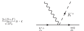
   Figure 1: Feynman rules for evaluating the $\Sigma^{+}$ electromagnetic polarizaibilities.

Appendix B Loop Integrals

Here, we have defined all the loop functions which occur in our calculation and we have given these functions in closed analytical form as far as possible. In the following all propagators are understood to have an infinitesimal imaginary part. The results of the integral are for real photons. The complete list of integrals can be found in BER95 :

$$\int\frac{d^{d}k}{(2\pi)^{d}i}\frac{1}{M^{2}_{P}-k^{2}}\ =\ \Delta_{P}$$ (23)

where

$$\Delta_{P} = 2M^{2}_{P}[L+\frac{1}{16\pi^{2}}\log\Big{(}\frac{4\pi}{\lambda}\Big{)}+{\cal O}(d-4)]\,,$$

$$L = \frac{\lambda^{d-4}}{16{\pi^{2}}}[\frac{1}{d-4}+\frac{1}{2}(\gamma_{E}-1-\log(4\pi)]$$ (24)

has a pole at $d=4$. Here P=$\pi$ or $K$, $\gamma_{E}=0.557215$ and $\lambda$ is the scale in dimensional regularization scheme used in the evaluation of integrals.

The relevant integrals are

$$\int\frac{d^{d}k}{(2\pi)^{d}i}\frac{(1,k^{\mu},k^{\mu}k^{\nu})}{(v\cdot k-\omega)[M_{P}^{2}-k^{2}]} = (J^{P}_{0}(\omega),v_{\mu}J^{P}_{1}(\omega),g^{\mu\nu}J^{P}_{2}(\omega)+v^{\mu}v^{\nu}J^{P}_{3}(\omega))\,,$$ (25)

where

$$J^{P}_{0}(\omega) = -4L{\omega}+\frac{\omega}{8{\pi}^{2}}(1-2\log\frac{M_{P}}{\lambda})-\frac{1}{4{\pi}^{2}}{\sqrt{M^{2}_{P}-{\omega}^{2}}}\arccos\Big{(}-\frac{\omega}{M_{P}}\Big{)}+{\cal O}(d-4)\,,$$ (26)

$$J^{P}_{1}(\omega) = {\omega}J^{P}_{0}(\omega)+\Delta_{P}\,,$$ (27)

$$J^{P}_{2}(\omega) = \frac{1}{d-1}[(M^{2}_{P}-{\omega}^{2})J^{P}_{0}(\omega)-{\omega}{\Delta_{P}}]\,,$$ (28)

$$J^{P}_{3}(\omega) = {\omega}J^{P}_{1}(\omega)-J^{P}_{2}(\omega)\,.$$ (29)

Appendix C ${\Sigma}^{+}{\pi}^{+}(K^{+})$ loops in forward Compton scattering

Using the loop integrals defined in Appendix B, the ${\Sigma^{+}}+{\pi}^{+}(K^{+})$ loop diagrams of Fig. 2 can be written as:

$${\rm Amp}^{{\Sigma}^{+}{\pi}^{+}}_{a+a^{\prime}} = C_{1}[S\cdot{\epsilon}^{*},S\cdot{\epsilon}][J^{\pi}_{0}(\omega)-J^{\pi}_{0}(-\omega)]$$ (30)

$${\rm Amp}^{{\Sigma}^{+}{\pi}^{+}}_{b+c+b^{\prime}+c^{\prime}} = C_{2}[S\cdot{\epsilon}^{*},S\cdot{\epsilon}]\frac{\partial}{{\partial}M^{2}_{\pi}}\int^{1}_{0}[J^{\pi}_{2}({\omega}z)-J^{\pi}_{2}(-{\omega}z)]dz$$ (31)

$${\rm Amp}^{{\Sigma}^{+}{\pi}^{+}}_{d+d^{\prime}} = D_{1}[S\cdot{\epsilon}^{*},S\cdot{\epsilon}][J^{\pi}_{0}(\omega)-J^{\pi}_{0}(-\omega)]\,,$$ (32)

$${\rm Amp}^{{\Sigma}^{+}{\pi}^{+}}_{e+f+e^{\prime}+f^{\prime}} = D_{2}[S\cdot{\epsilon}^{*},S\cdot{\epsilon}]\frac{\partial}{{\partial}M^{2}_{\pi}}\int^{1}_{0}[J^{\pi}_{2}({\omega}z)-J^{\pi}_{2}(-{\omega}z)]dz\,,$$ (33)

$${\rm Amp}^{{\Sigma}^{+}{K}^{+}}_{g+g^{\prime}} = E_{1}[S\cdot{\epsilon}^{*},S\cdot{\epsilon}][J^{K}_{0}(\omega)-J^{K}_{0}(-\omega)]\,$$ (34)

$${\rm Amp}^{{\Sigma}^{+}{K}^{+}}_{h+i+h^{\prime}+i^{\prime}} = E_{2}[S\cdot{\epsilon}^{*},S\cdot{\epsilon}]\frac{\partial}{{\partial}M^{2}_{K}}\int^{1}_{0}[J^{K}_{2}({\omega}z)-J^{K}_{2}(-{\omega}z)]dz\,,$$ (35)

where

$$C_{1} = 2i\,\Big{(}\frac{e\,F}{F_{0}}\Big{)}^{2}\,,\quad C_{2}\ =\ -8i\,\Big{(}\frac{e\,F}{F_{0}}\Big{)}^{2}\,,$$ (36)

$$D_{1} = \frac{2i}{3}\,\Big{(}\frac{e\,D}{F_{0}}\Big{)}^{2}\,,\quad D_{2}\ =\ -\frac{8i}{3}\,\Big{(}\frac{e\,D}{F_{0}}\Big{)}^{2}\,,$$ (37)

$$E_{1} = i\,\Big{(}\frac{e\,(D+F}{F_{0}}\Big{)}^{2}\,,\quad E_{2}\ =\ -4i\,\Big{(}\frac{e\,(D+F}{F_{0}}\Big{)}^{2}\,.$$ (38)

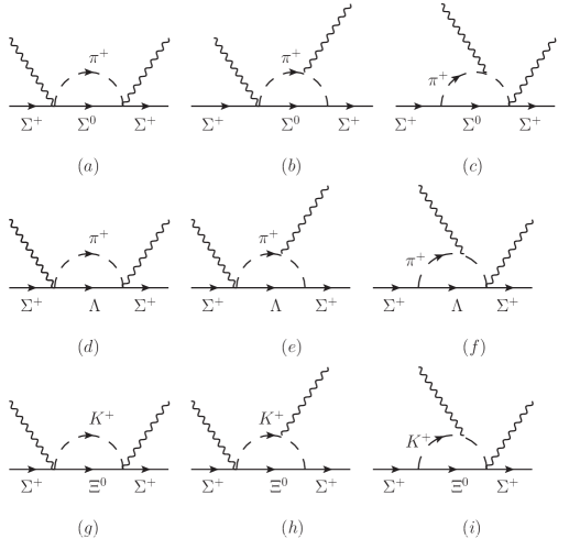
Figure 2: The one loop diagrams contributing to forward Compton scattering of $\Sigma^{+}$ $\pi^{+}$ $(K^{+})$ at $O(p^{3})$. Crossed diagrams are not shown.

Table 1: The forward spin polarizablity $\gamma_{0}$ of octet baryons (in units of $10^{-4}$ fm⁴)

Baryon	Our results at $O(p^{3})$	Our results at $O(p^{3})$	$O(p^{3})\,$	$O(p^{4})\,$
	with $\pi$ loops	with $\pi$ and $K$ loops	HBChPT BER92	HBChPT and BChPT	Electroproduction data
$p$	4.50	4.86	4.5	$4.5-(6.9+1.5)$ KBV2000 ; XJ2000 ; GCG2000 , 4.64 BER03	$-$1.3 AMS94 ,  $-$0.6 DD98one ,
					$-0.58\pm 0.2$ SCH2011
$n$	4.50	4.86	4.5	$4.5-(6.9-1.5)$ KBV2000 ; XJ2000 ; GCG2000 , 1.82 BER03	$-$0.4 AMS94 ,
					$-0.38\pm 0.22$ SCH2011
$\Sigma^{+}$	1.20	1.38
$\Sigma^{0}$	0.60	0.70
$\Sigma^{-}$	1.20	1.22
$\Lambda$	0.60	0.70
$\Xi^{-}$	0.16	0.26
$\Xi^{0}$	0.16	0.43

References

• (1) A.Β M.Β Baldin, Nucl.Β Phys.Β 18, Β 310 (1960).
• (2) B.Β R.Β Holstein, Comments Nucl.Β Part.Β Phys.Β  20, 301 (1992)
• (3) B.Β R.Β Holstein and A.Β M.Β Nathan, Phys.Β Rev.Β  D 49, 6101 (1994) [arXiv:hep-ph/9402248].
• (4) V.Β Bernard, N.Β Kaiser and U.Β G.Β Meissner, Int.Β J.Β Mod.Β Phys.Β  E4, 193 (1995) [arXiv:hep-ph/9501384].
• (5) B.Β W.Β Filippone and X.Β D.Β Ji, Adv.Β Nucl.Β Phys.Β  26, 1 (2002) [arXiv:hep-ph/0101224].
• (6) D.Β Drechsel, B.Β Pasquini and M.Β Vanderhaeghen, Phys.Β Rept.Β  378, 99 (2003) [arXiv:hep-ph/0212124].
• (7) M.Β Schumacher, Prog.Β Part.Β Nucl.Β Phys.Β  55, 567 (2005) [arXiv:hep-ph/0501167].
• (8) B.Β Pasquini, D.Β Drechsel and M.Β Vanderhaeghen, [arXiv:hep-ph/1105.4454 ].
• (9) K.Β Nakamura et al. (Particle Data Group), J.Β Phys.Β G 37, 075021 (2010).
• (10) W.Β Pfeil, H.Β Rollnik and S.Β Stankowski, Nucl.Β Phys.Β  B 73, 166 (1974).
• (11) I.Β Guiasu, C.Β Pomponiu and E.Β E.Β Radescu, Annals Phys.Β  114, 296 (1978).
• (12) A.Β I.Β Lvov, Sov.Β J.Β Nucl.Β Phys.Β  34, 597 (1981) [Yad.Β Fiz.Β  34, 1075 (1981)].
• (13) A.Β I.Β L’vov, V.Β A.Β Petrun’kin and M.Β Schumacher, Phys.Β Rev.Β  C 55, 359 (1997).
• (14) D.Β Drechsel, M.Β Gorchtein, B.Β Pasquini and M.Β Vanderhaeghen, Phys.Β Rev.Β  C 61, 015204 (1999) [arXiv:hep-ph/9904290].
• (15) B.Β Pasquini, D.Β Drechsel and M.Β Vanderhaeghen, Phys.Β Rev.Β  C 76, 015203 (2007) [arXiv:hep-th/0705.0282].
• (16) V.Β Pascalutsa and O.Β Scholten, Nucl.Β Phys.Β  A 591, 658 (1995).
• (17) O.Β Scholten, A.Β Y.Β Korchin, V.Β Pascalutsa and D.Β Van Neck, Phys.Β Lett.Β  B 384, 13 (1996) [arXiv:nucl-th/9604014].
• (18) T.Β Feuster and U.Β Mosel, Phys.Β Rev.Β  C 59, 460 (1999) [arXiv:nucl-th/9803057].
• (19) S.Β Kondratyuk and O.Β  Scholten, S.Β Kondratyuk and O.Β Scholten, Nucl.Β Phys.Β  A 677, 396 (2000) [arXiv:nucl-th/0003009]; S.Β Kondratyuk and O.Β Scholten, Phys.Β Rev.Β  C 64, 024005 (2001) [arXiv:nucl-th/0103006].
• (20) S.Β I.Β Kruglov, Hadronic J.Β Suppl.Β  17, 103 (2003) [arXiv:hep-ph/0110101].
• (21) S.Β Capstick and B.Β D.Β Keister, Phys.Β Rev.Β  D 46, 84 (1992) [Erratum-ibid.Β  D 46, 4104 (1992)] [Phys.Β Rev.Β  D 46, 4104 (1992)].
• (22) H.Β Liebl and G.Β R.Β Goldstein, Phys.Β Lett.Β  B 343, 363 (1995) [arXiv:hep-ph/9411230].
• (23) Y.Β B.Β Dong, A.Β Faessler, T.Β Gutsche, J.Β Kuckei, V.Β E.Β Lyubovitskij, K.Β Pumsa-ard and P.Β N.Β Shen, J.Β Phys.Β G 32, 203 (2006) [arXiv:hep-ph/0507277].
• (24) M.Β Chemtob, Nucl.Β Phys.Β  A 473, 613 (1987).
• (25) N.Β N.Β Scoccola and W.Β Weise, Phys.Β Lett.Β  B 232, 287 (1989).
• (26) S.Β Scherer and P.Β J.Β Mulders, Nucl.Β Phys.Β  A 549, 521 (1992).
• (27) W.Β Broniowski and T.Β D.Β Cohen, Phys.Β Rev.Β  D 47, 299 (1993) [arXiv:hep-ph/9208256].
• (28) N.Β N.Β Scoccola and T.Β D.Β Cohen, Nucl.Β Phys.Β  A 596, 599 (1996) [arXiv:hep-ph/9507328].
• (29) F.Β X.Β Lee, L.Β Zhou, W.Β Wilcox and J.Β C.Β Christensen, Phys.Β Rev.Β  D 73, 034503 (2006) [arXiv:hep-lat/0509065].
• (30) W.Β Detmold, B.Β C.Β Tiburzi and A.Β Walker-Loud, Phys.Β Rev.Β  D 73, 114505 (2006) [arXiv:hep-lat/0603026]; W.Β Detmold, B.Β C.Β Tiburzi and A.Β Walker-Loud, Phys.Β Rev.Β  D 81, 054502 (2010) [arXiv:hep-lat/1001.1131 ].
• (31) M.Β Engelhardt [LHPC Collaboration], Phys.Β Rev.Β  D 76, 114502 (2007) [arXiv:hep-lat/0706.3919 ].
• (32) S.Β Weinberg, Physica A 96, 327 (1979).
• (33) J.Β Gasser and H.Β Leutwyler, Annals Phys.Β  158, 142 (1984); J.Β Gasser and H.Β Leutwyler, Nucl.Β Phys.Β B 250, 465 (1985).
• (34) E.Β E.Β Jenkins and A.Β V.Β Manohar, Phys.Β Lett.Β  B 255, 558 (1991).
• (35) E.Β E.Β Jenkins, Nucl.Β Phys.Β  B 368, 190 (1992).
• (36) V.Β Bernard, N.Β Kaiser and U.Β G.Β Meissner, Phys.Β Rev.Β Lett.Β  67, 1515 (1991).
• (37) V.Β Bernard, N.Β Kaiser and U.Β G.Β Meissner, Nucl.Β Phys.Β  B 373, 346 (1992).
• (38) T.Β Becher and H.Β Leutwyler, Eur.Β Phys.Β J.Β  C 9, 643 (1999) [arXiv:hep-ph/9901384].
• (39) V.Β Lensky and V.Β Pascalutsa, Pisma Zh.Β Eksp.Β Teor.Β Fiz.Β  89, 127 (2009) [JETP Lett.Β  89, 108 (2009)] [arXiv:nucl-th/0803.4115 ].
• (40) V.Β Lensky and V.Β Pascalutsa, Eur.Β Phys.Β J.Β  C 65, 195 (2010) [arXiv:hep-ph /0907.0451 ].
• (41) D.Β Drechsel, G.Β Knochlein, A.Β Y.Β Korchin, A.Β Metz and S.Β Scherer, Phys.Β Rev.Β  C 58, 1751 (1998) [arXiv:nucl-th/9804078].
• (42) T.Β R.Β Hemmert, B.Β R.Β Holstein, G.Β Knochlein and S.Β Scherer, Phys.Β Rev.Β  D 55, 2630 (1997) [arXiv:nucl-th/9608042]; T.Β R.Β Hemmert, B.Β R.Β Holstein, G.Β Knochlein and S.Β Scherer, Phys.Β Rev.Β Lett.Β  79, 22 (1997) [arXiv:nucl-th/9705025].
• (43) T.Β R.Β Hemmert, B.Β R.Β Holstein, J.Β Kambor and G.Β Knochlein, Phys.Β Rev.Β  D 57, 5746 (1998) [arXiv:nucl-th/9709063].
• (44) T.Β R.Β Hemmert, B.Β R.Β Holstein, G.Β Knochlein and D.Β Drechsel, Phys.Β Rev.Β  D 62, 014013 (2000) [arXiv:nucl-th/9910036].
• (45) S.Β R.Β Beane, M.Β Malheiro, J.Β A.Β McGovern, D.Β R.Β Phillips and U.Β van Kolck, Nucl.Β Phys.Β  A 747, 311 (2005) [arXiv:nucl-th/0403088].
• (46) A.Β C.Β Hearn and E.Β Leader, Phys.Β Rev.Β  126, 789 (1962).
• (47) T.Β R.Β Hemmert, B.Β R.Β Holstein, J.Β Kambor and G.Β Knochlein, Phys.Β Rev.Β  D 57, 5746 (1998) [arXiv:nucl-th/9709063].
• (48) B.Β R.Β Holstein, Acta Phys.Β Polon.Β  B 29, 2467 (1998) [arXiv:nucl-th/9806035].
• (49) S.Β R.Β Beane, M.Β Malheiro, J.Β A.Β McGovern, D.Β R.Β Phillips and U.Β van Kolck, Phys.Β Lett.Β  B 567, 200 (2003) [Erratum-ibid.Β  B 607, 320 (2005)] [arXiv:nucl-th/0209002].
• (50) F.Β E.Β Low, Phys.Β Rev.Β  96, 1428 (1954); M.Β Gell-Mann and M.Β L.Β Goldberger, Phys.Β Rev.Β  96, 1433 (1954).
• (51) V.Β Bernard, N.Β Kaiser, J.Β Kambor and U.Β G.Β Meissner, Nucl.Β Phys.Β  B 388, 315 (1992).
• (52) K.Β B.Β Vijaya Kumar, J.Β A.Β McGovern and M.Β C.Β Birse, Phys.Β Lett.Β  B 479, 167 (2000) [arXiv:hep-ph/0002133].
• (53) X.Β D.Β Ji, C.Β W.Β Kao and J.Β Osborne, Phys.Β Lett.Β  B 472, 1 (2000) [arXiv:hep-ph/9910256].
• (54) G.Β C.Β Gellas, T.Β R.Β Hemmert and U.Β G.Β Meissner, Phys.Β Rev.Β Lett.Β  85, 14 (2000) [arXiv:nucl-th/0002027]; G.Β C.Β Gellas, T.Β R.Β Hemmert and U.Β G.Β Meissner, Phys.Β Rev.Β Lett.Β  86, 3205 (2001).
• (55) M.Β C.Β Birse, X.Β D.Β Ji and J.Β A.Β McGovern, Phys.Β Rev.Β Lett.Β  86, 3204 (2001) [arXiv:nucl-th/0011054].
• (56) V.Β Bernard, T.Β R.Β Hemmert and U.Β G.Β Meissner, Phys.Β Rev.Β  D 67, 076008 (2003) [arXiv:hep-ph/0212033].
• (57) C.Β W.Β Kao, Int.Β J.Β Mod.Β Phys.Β  A 21, 2027 (2006).
• (58) A.Β M.Β Sandorfi, M.Β Khandaker and C.Β S.Β Whisnant, Phys.Β Rev.Β  D 50, R6681 (1994).
• (59) D.Β Drechsel, G.Β Krein and O.Β Hanstein, Phys.Β Lett.Β  B 420, 248 (1998) [arXiv:nucl-th/9710029].
• (60) M.Β Schumacher, [arXiv:hep-ph/1104372].
• (61) M.Β Schumacher, Nucl.Β Phys.Β A 826,131 (2009) [arXiv:hep-ph/09054363] .
• (62) B.Β Pasquini,P.Β Pedroni,D.Drechsel,Phys.Β Lett.Β B 687, 160 (2010) [arXiv:hep-ph/10014230].
• (63) V.Β Bernard, N.Β Kaiser, J.Β Kambor and U.Β G.Β Meissner, Phys.Β Rev.Β  D 46, R2756 (1992).
• (64) V.Β A.Β Petrunkin, Fiz.Β Elem.Β Chast.Β Atom.Β Yadra 12, 692 (1981) [Sov.Β J.Β Part.Β Nucl.Β 12, 278 (1981)].
• (65) H.Β J.Β Lipkin and M.Β A.Β Moinester, Phys.Β Lett.Β  B 287, 179 (1992).
• (66) C.Β Gobbi, C.Β L.Β Schat and N.Β N.Β Scoccola, Nucl.Β Phys.Β  A 598, 318 (1996) [arXiv:hep-ph/9509211].
• (67) T.Β Nishikawa, S.Β Saito and Y.Β Kondo, Phys.Β Lett.Β  B 422, 26 (1998) [arXiv:hep-ph/9710435].
• (68) Y.Β Tanushi,Β S.Β Saito and M.Β Uehara,Β Phys.ReV.Β C61,055204 (2000) Y.Β Tanushi, S.Β Saito and M.Β Uehara, Phys.Β Rev.Β  C 61, 055204 (2000) [arXiv:nucl-th/9911071].
• (69) A.Β Aleksejevs and S.Β Barkanova, J.Β Phys.Β G 38, 035004 (2011) [arXiv:nucl-th/1010.3457 ].