On the Evaluation Criterions for the Active Learning Processes

Abstract

In many data mining applications collection of sufficiently large datasets is the most time consuming and expensive. On the other hand, industrial methods of data collection create huge databases, and make difficult direct applications of the advanced machine learning algorithms. To address the above problems, we consider active learning (AL), which may be very efficient either for the experimental design or for the data filtering. In this paper we demonstrate using the online evaluation opportunity provided by the AL Challenge that quite competitive results may be produced using a small percentage of the available data. Also, we present several alternative criteria, which may be useful for the evaluation of the active learning processes. The author of this paper attended special presentation in Barcelona, where results of the WCCI 2010 AL Challenge were discussed.

Keywords: unlabeled data, semi supervised learning, random sets

1 Introduction

Traditional supervised learning algorithms use whatever labeled data is provided to construct a model. By contrast, active learning gives the learner a degree of control by allowing the selection of labeled instances to be added to the training set [1]. One of the most popular methods of AL is uncertainty sampling, where the learner queries the instance about which it has the least certainty [2], or query-by-committee, where a “committee” of models selects the instance about which its members most disagree [3].

Based on our experience, we can divide the AL process into three main periods: 1) initial, which may be characterised by a high level of volatility, because of the lack of information; 2) actual, during which significant progress may be made, and 3) validation, which may be implemented, for example, using random sampling.

We claim that any intermediate results during an initial period are not important, because these results are based on insufficient evidence. However, the outcome of the initial period is significant as it represents a starting point for the following most important period of actual AL.

During the second period of actual AL, it is essential for the learning system to demonstrate speed and consistency of the improvement, and we can use a variety of methods to check convergence of the learning process. After we have found that the results are satisfactory, we can collect at random a large amount of labels and we can evaluate the learning trajectory (see Figures 3 and  4). Rows “AUC”, “ALC” and “AUC-rand”, “ALC-rand” of Table 1 demonstrate similarity between the final (official) results and the corresponding results, which were evaluated using random sampling.

AL may be implemented through very interesting and sophisticated methods [4, 5]. Unfortunately, it is most unlikely that these methods would be very efficient in this particular Challenge because of the problems with the evaluation criterion (see Section 3 for more details).

Some interesting papers including report of the Organisers of the WCCI 2010 AL Challenge [6] maybe downloaded for free from the web-site of the Journal of Machine Learning Research.

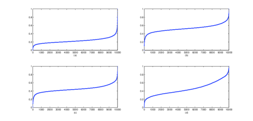
Figure 1: Sorted decision functions corresponding to the set D: (a) step 2; (b) step 5; (c) step 12 and (d) step 16.

2 Task Description and Methods

In many applications, including handwriting recognition, chemo-informatics, and text processing, large amounts of unlabeled data are available at low cost, but labeling examples (using a human expert to find the corresponding labels) is tedious and expensive. Hence there is a benefit either to use unlabeled data to improve the model in a semi supervised learning algorithm [7, 8], or to sample efficiently and to use human expertise for labeling only the most informative examples.

Six tasks named A, B, C, D, E, and F of pool-based active learning were considered during the AL Challenge, in which large unlabeled datasets are available from the outset of the Challenge and the participants can place queries to acquire data for some amount of virtual cash. The participants need to return prediction values for all the labels every time they want to purchase new labels. This allows the Organisers to draw learning curves of prediction performance versus the amount of virtual cash spent. The participants are judged according to the area under the learning curves (3).

Table 1: Some statistical characteristics related to the Sets A-F and to the methods, which we used during the AL Challenge.

DataSet	A	B	C	D	E	F
Sample size	17535	25000	25720	10000	32252	67628
No of submissions	13	17	16	17	13	13
Used samples	811	1101	2301	531	661	900
Percentage	4.63$\%$	4.40$\%$	8.95$\%$	5.31$\%$	2.05$\%$	1.33$\%$
Last weight	4.32	4.51	3.48	4.24	5.61	6.23
Validation	900	1200	2000	1000	800	1999
Percent (positives)	30.95$\%$	17.98$\%$	16.71$\%$	39.36$\%$	18.76$\%$	27.86$\%$
$AUC_{1}$	0.5177	0.6304	0.4988	0.5098	0.5613	0.6179
$AUC$	0.8847	0.7323	0.7766	0.9404	0.7457	0.9853
$ALC$	0.4775	0.2834	0.2378	0.602	0.3689	0.6517
$ALC_{2}$	0.5178	0.3941	0.3415	0.5874	0.3761	0.7456
Percent (positives) -rand	20.89$\%$	8$\%$	8.85$\%$	25.7$\%$	11.75$\%$	7.25$\%$
$AUC$ - rand	0.8929	0.7326	0.7854	0.9334	0.7501	0.9843
$ALC$ - rand	0.4682	0.2915	0.2367	0.6038	0.3417	0.6398

2.1 Uncertainty Sampling

At the beginning of the AL Challenge, we were given only one labeled (positive) sample. We decided to use an assumption that the data are highly imbalanced with smaller number of positive instances. Accordingly, we considered for the first step 50-100 random sets with given positive sample and other samples (assumed to be negative), which were selected randomly, but under condition that they are sufficiently distant from the given positive instance. The decision function was calculated as a sample average. We continued to use similar random sampling in the further steps, but the proportion of the randomly selected instances was smaller. After 4-6 steps we stopped using random sampling. The query for a new label was carried out according to the structure of the decision function, which was sorted in increasing order; see Figure 1.

We decided that the most appropriate selection of the samples in order to make a query is the range, where the decline of the decision function is changing from the rapid to smoothed. As a consequence, the fractions of the positive samples in our training sets were significantly higher compared to the fractions of the positive samples in the validation sets, which were collected randomly; see rows “Percent (positive)” and “Percent (positive) - rand”, Table 1.

During the initial few steps, we used as a classifier the kridge function from the CLOP package. After collecting more labels, we started experiments with other functions: neural (also from CLOP package); $GLM$, $ADA$, and $GBM$ from $R$. Also, we conducted feature selection using the Wilcoxon criterion for the Sets A, B, C and E; and a special likelihood-based criterion (binary) was used in application to the Set D. Below the level of 200-300 of the labeled samples, we used LOO for the evaluation and optimisation of the used parameters. Then, we conducted experiments using CV with 10-20 folds. The final decision function was computed as an ensemble of the base decision functions, where particular weights were defined according to the results of the evaluations with CV.

On the final phase of our experiment, we collected at random sufficiently large sample for the evaluation of our learning curve (the sizes of the validation samples are given in the row “Validation”, Table 1).

2.2 An ensemble constructor (a general approach)

Definition 1

An ensemble is defined as heterogeneous if the base models in an ensemble are generated by methodologically different learning algorithms (we shall consider such an ensemble in this Section). On the other hand, an ensemble is defined as homogeneous if the base models are of the same type (for example, boosting or random forest).

Suppose, we have two high quality solutions, which are very different. Obviously, a direct sample average will not be efficient in this particular case.

The following very simple Matlab code may be very useful in order to adjust one solution to the scale of the other solution without any loss of quality.

[a1,f1]=sort(x1);   - solution N1
[a2,f2]=sort(x2);   - solution N2
[b2,g2]=sort(f2);
x3=x1;
for i=1:size(x1,1),
    ii=g2(i);
    x3(i)=a1(ii);   - adjusted solution
end;

After the above adjustment, we can compute an ensemble solution as a linear combination:

$$x_{ens}=\tau\cdot x_{1}+(1-\tau)\cdot x_{3}$$ (1)

of the input solutions $x_{1}$ and $x_{3},$ where $0<\tau<1$ is a positive weight coefficient. Clearly, the stronger performance of the solution $x_{1}$ compared to $x_{3}$, the bigger will be the value of the coefficient $\tau.$

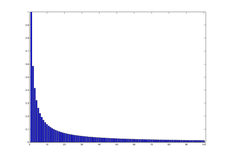
Figure 2: Behavior of the weight function $w,$ which is defined in (3).

3 ALC Criterion

Suppose, we have a sequence: $n_{i},i=1,\ldots,N$ - to be the sizes of the requests, where $n_{1}=1$; $t_{i}=\sum_{j=1}^{i}n_{j}$ - the corresponding training sizes.

By definition, the area under learning curve (ALC) is

$$ALC=\frac{2}{\log_{2}{(T)}}\sum_{i=1}^{N}\widehat{AUC}_{i}\log_{2}{\frac{t_{i+1}}{t_{i}}}-1,$$ (2)

where

$$\widehat{AUC}_{i}=\frac{AUC_{i}+AUC_{i+1}}{2},$$

$\hskip 3.61371ptAUC_{N+1}=AUC_{N},t_{N+1}=T$ is the total available sample size (see row “Sample size” in Table 1).

In order to simplify further notation, suppose that $n_{i}=n_{2}+1,i=3,\ldots,N,N\geq 3.$ Then, the criterion ALC, which is given by equation (2) may be rewritten in the following form,

$$ALC\sim\widehat{AUC}_{1}\log_{2}{(n_{2}+1)}+\sum_{i=2}^{N-1}\widehat{AUC}_{i}w_{i}+AUC_{N}\log_{2}{\frac{T}{t_{N}}},$$ (3)

where

$$w_{i}=\log_{2}{(1+\frac{1}{i-1})},$$

and we ignore in (3) the linear and shift coefficients as they do not make any difference to the classification of the learning curves.

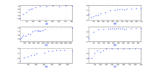
Figure 3: Trajectories in terms of AUCs corresponding to the Sets A-F.

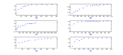
Figure 4: Trajectories in terms of ALC’s corresponding to the Sets A-F.

Figure 2 illustrates the rapid decline in the coefficients $w_{i},i=2,\ldots,N.$ But the real winner in this particular Challenge was the first coefficient $w_{1}=\log_{2}{(n_{2}+1)}.$ In all our submissions, we used $n_{2}=50,$ which corresponds to $w_{1}\approx 5.67.$ Values corresponding to the last coefficient

$$w_{N}=\log_{2}{\frac{T}{t_{N}}}$$

are presented in the row “Last weight”, Table 1. Only in the case of Set F, where we used $1.33\%$ of all available data, the last term is slightly more important compared to the first term. In all other cases the first term is the most important. Given that we did not use more that $9\%$ of all available data, this fact appears to be very surprising.

During the AL Competition, we acted in accordance with the natural logic (learn carefully with small steps). We had no time to practice with the development sets before the Competition in order to discover some essential features of the criterion (2).

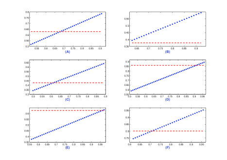
Figure 5: ALCs as a function of the first entry (see for more details Section 3.2). The exact values of the lowest points (blue dotted lines) are given in the row “$ALC_{2}$”, Table 1.

3.1 Illustration

Figures 3(F) and  4(F) illustrate the fact that the first two values (vertical points) of the trajectories corresponding to the set F are equal. This happened accidentally because we submitted solution from the wrong directory. In this particular Challenge such a mistake was very serious. In order to check sensitivity of the ALC evaluation criterion, we replaced the second value by the average of first and third values. As a result, the ALC grew from $0.6517$ to $0.6842.$

3.2 Special binary case: N=2

After the results of the competition were released, we noticed that binary strategies with only two entries (or with the first step as a very big jump) were very popular. The motivation for such an approach is very simple. As it discussed in Section 3, it is extremely important to maximise $\widehat{AUC}_{1},$ because of the given evaluation criterion (2).

One way to do this is through the cooperation between different teams (formally it is restricted, but cannot be controlled with full certainty). The second way is to collect at random a very large sample, for example, $5-10\%$ of all available data (to ensure sufficiently large value of $AUC_{2}$). Probably, that was the best choice during this Challenge. In fact, we have found that the criterion (2) does not encourage, but discourage the process of actual AL.

Let us consider more detailed illustration for the above fact. In the case $N=2$ we can rewrite (2) in the following simplified form:

$$ALC_{2}=\frac{2}{\log_{2}{(T)}}\left(\frac{AUC_{1}+AUC_{2}}{2}\log_{2}{(t_{2})}+AUC_{2}\log{\frac{T}{t_{2}}}\right)-1.$$ (4)

Figure 5 illustrates behaviour of $ALC_{2}$ as a function of $AUC_{1},$ where the left (smallest) horizontal point corresponds to our initial AUC-score, values of $t_{2}$ are given in the row “Used samples”, values of $AUC_{2}$ are given in the row “AUC”, Table 1.

Remark 2

We were able to observe that such dramatic simplification of the strategy led to improvement of the winning ALC score for Set B (we do believe that we will be able to reproduce our final result of 0.7323 using 1101 randomly selected labeled instances). All results corresponding to the binary strategy with our initial and final AUC scores are given in the row “$ALC_{2}$”, Table 1, where only in the case of Set D the result was slightly worse compared to our final result for Set D.

Remark 3

Normally, it is unlikely to expect that an initial AUC score based on only one labeled point will be better than 0.55. We do believe, if an initial result were greater than 0.65, there must be some problems with the data or competitor who generated such result used some additional information, which was restricted by the rules of the Challenge. Our initial AUC-scores are given in the row “$AUC_{1}$”, Table 1.

3.3 Optimal size of the request in the binary case

It will be more convenient to rewrite equation (4) in the following form

$$ALC_{2}(t)\sim\frac{\log_{2}{(t)}}{2}(AUC_{1}-AUC_{2}(t))+AUC_{2}(t)\log_{2}{(T)},$$ (5)

where $ALC_{2}(t)$ is an increasing function of $1\leq t\leq T$: $AUC_{1}=AUC_{2}(1).$

Suppose that based on the arguments and considerations of the previous section we decided to select a binary strategy, and our task is to maximise (5).

Figure 3 illustrates that after some point the behaviour of the AUC graphs become nearly stable, and there are no sense to go further, because the above target function (5) will decline slowly at the logarithmic rate.

The main question is how to define the optimal stopping point. In the case where the competitor follows correctly the second period of actual AL with small steps, this problem will be solved naturally by comparing the current and several previous solutions. But the competitor will face an extra penalty as a result of the small steps during initial period. So in this particular Challenge the random selection of the $5\%-10\%$ of the available labels will be fine and the most appropriate (“the first step as a big jump”). As we can see, the competitor is strongly encouraged to avoid the most important period of actual AL: just make a big jump, and there are absolutely no any sense to do anything after that.

It is most unlikely that the Organisers would have used the evaluation criterion (2) if they had had this paper in hand before.

4 Two Proposed Evaluation Criteria

4.1 Formulation of the framework related to the modified criterion

Our target is to produce better classification accuracy with a smaller number of labeled examples.

The learning process includes two subintervals (in accordance to the number of the used labels):

1) The first subinterval in which the number of labeled instances is less than $\delta$ (for example, $\delta$ may be $1\%$ of all data available and (anyway) not more than 200). This subinterval will not be counted for the Challenge.

2) The second subinterval of the actual AL after $\delta.$ This subinterval will be counted for the Challenge.

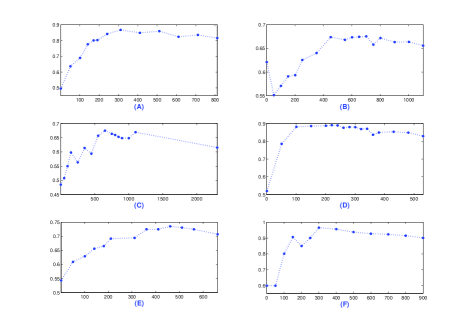
Figure 6: The same trajectories as in Figure 3, evaluated with criterion (6).

4.2 Motivation

In an industrial sense, any decision making based on a small number of labeled instances cannot be regarded as a serious. Any results, which are based on a small number of labeled instances, have no sufficient grounds to be implemented (and, probably, may only give some directions for further studies).

The main idea: it is not important how the participant will grow to the level of $\delta$, the actual learning and savings will be started after that.

4.3 Second proposed criterion

Let us consider

$$Q=\max_{i=1,\ldots,N}\frac{\delta\cdot AUC_{i}}{\delta+\alpha\cdot\max{(0,t_{i}-\delta)}},$$ (6)

where $\delta>0$ and $\alpha>0$ are regulation parameters.

Example

Similarly as in Section 4.1, we can select the threshold $\delta$ in (6) as $1\%$ of $T$ : $\delta=0.01\cdot T.$

Suppose that $A$ and $B$ are the expected values of AUC corresponding to $\delta$ and $\Delta,$ where $\Delta$ is $20\%$ of $T$ : $\Delta=0.2\cdot T$ (for example, B = 1.5 A).

The following equation follows from (6),

$$\frac{A}{\delta}=\frac{B}{\delta+\alpha(\Delta-\delta)}.$$

Therefore,

$$\alpha=\frac{\delta}{\Delta-\delta}\left(\frac{B}{A}-1\right)=\frac{1}{38}.$$

Note that all graphs in Figure 6 were computed using the same regulation parameters as in this section.

Remark 4

The criterion (6) will impose equal penalties on any solution made within the level of $\delta.$ After that level, the penalty will grow. However, the quality of the solution will grow as well, and the task is not to stop earlier, because using “big jumps” the competitors will face the risk to miss an optimal point. Therefore, criterion (6) will encourage actual AL with many steps, which must be reasonably small.

5 Concluding Remarks

As it was noticed in [9], if the improvement of a quantitative criterion such as the error rate is the main contribution of a paper, the superiority of a new algorithms should always be demonstrated on independent validation data. In this sense, an importance of the data mining contests is unquestionable. The rapid popularity growth of the data mining challenges demonstrates with confidence that it is the best known way to evaluate different models and systems.

While the idea of AL appears to be very promising, we think that it is not a quite suitable subject for data mining competitions, because of the difficulties to check the independence of the learning processes. As it was discussed in this paper (and during intensive email correspondence shortly after results were released), we do believe that the evaluation criterion that was used during the AL Challenge severely overestimated importance of the initial learning period. The first step (based on one labeled sample) was the most important. In the case where this step was unsuccessful, it was not possible to compensate the loss by the further steps. On the other hand, if we know that the first submission was strong, we can request a large (at random) amount of labels and the success at the second step (and the final success) will be guaranteed.

Our criticism is a constructive, and we have proposed two ways how to improve the evaluation criterion, which is the topic of the primary importance for any competition.

Acknowledgments

This work was supported by a grant from the Australian Research Council. Also, we are grateful to the Organisers of the WCCI 2010 AL data mining Contest for this stimulating opportunity.

References

- [1] Settles B. and Craven M. “An Analysis of Active Learning Strategies for Sequence Labeling Tasks.” Proceedings of the Conference on Empirical Methods in Natural Language Processing, pp. 1070-1079, 2008.
- [2] Culotta A. and McCallum A. “Reducing Labeling Effort for Structured Prediction Tasks.” Proceedings of the AAAI Conference, pp. 746-756, 2005.
- [3] Seung H., Opper M. and Sompolinsky H. “Query by Committee.” Proceedings of the COLT Conference, pp. 287-294, 1992.
- [4] Cohl D., Ghahramani Z. and Jordan M. “Active Learning with Statistical Models.” Journal of Artificial Intelligence Research, 4, pp. 129-145, 1996.
- [5] Tong S. and Koller D. “Active Learning for Parameter Estimation in Bayesian Networks.” Proceedings of the NIPS, 2001.
- [6] Guyon I., Cawley G., Dror G. and Lemaire V. “Results of the Active Learning Challenge.” JMLR:Workshop and Conference Proceedings, 16, pp. 19-45, 2011.
- [7] Kemp C., Griffiths T., Stromsten S. and Tenenbaum J. “Active Learning for Parameter Estimation in Bayesian Networks.” Proceedings of the NIPS, 2004.
- [8] Lafferty J. and Wasserman L. “Statistical Analysis of Semi-Supervised Regression.” Proceedings of the NIPS, 2008.
- [9] Jelizarow, M., Guillemot, V., Tenenhaus, A., Strimmer, K. and Boulesteix, A.-L. “Over-optimism in bioinformatics: an illustration.” Bioinformatics, 26(16), pp. 1990-1998, 2010.