$\alpha$-Modulation Spaces (I) Scaling, Embedding and Algebraic Properties

Abstract. First, we consider some fundamental properties including dual spaces, complex interpolations of $\alpha$-modulation spaces $M^{s,\alpha}_{p,q}$ with $0<p,q\leq\infty$. Next, necessary and sufficient conditions for the scaling property and the inclusions between $\alpha_{1}$-modulation and $\alpha_{2}$-modulation spaces are obtained. Finally, we give some criteria for $\alpha$-modulation spaces constituting multiplication algebra. As a by-product, we show that there exists an $\alpha$-modulation space which is not an interpolation space between modulation and Besov spaces. In a subsequent paper, we will give some applications of $\alpha$-modulation spaces to nonlinear dispersive wave equations.

Key words. $\alpha$-modulation space, Dual space, Multiplication algebra, Scaling property, Embedding.

AMS subject classifications. 42 B35, 42 B37, 35 A23

1 Introduction and definition

Frequency localization technique plays an important role in the modern theory of function spaces. There are two kinds of basic partitions to the Euclidean space $\mathbb{R}^{n}$, one is the dyadic decomposition $\mathbb{R}^{n}=\{\xi:|\xi|<1\}\bigcup(\bigcup^{\infty}_{j=1}\{\xi:|\xi|\in[2^{j-1},2^{j})\})$, another is the uniform decomposition $\mathbb{R}^{n}=\bigcup_{k\in\mathbb{Z}^{n}}(k+[-1/2,1/2)^{n})$. According to these two kinds of decompositions in frequency spaces, one can naturally introduce the dyadic decomposition operators $\triangle_{j}\ (j\in\mathbb{Z}_{+})$ whose symbol $\varphi_{j}$ is localized in $\{\xi:|\xi|\sim 2^{j}\}$, and the uniform decomposition operator $\square_{k}\ (k\in\mathbb{Z}^{n})$ whose symbol $\sigma_{k}$ is supported in $k+[-1,1]^{n}$. The difference between $\varphi_{j}$ and $\sigma_{k}$ is that the diameters of ${\rm supp}\ \varphi_{j}$ and ${\rm supp}\ \sigma_{k}$ are $O(2^{j})$ and $O(1)$, respectively. All tempered distributions acted on these decomposition operators with finite $\ell^{q}(L^{p})$ (quasi)-norms constitute Besov space $B_{p,q}^{s}$ and modulation space $M_{p,q}^{s}$, respectively.

The $\alpha$-modulation spaces $M_{p,q}^{s,\alpha}$, introduced by Gröbner [11], are proposed to be intermediate function spaces to connect modulation space and Besov space with respect to parameters $\alpha\in[0,1]$, which are formulated by some new kind of $\alpha$-decomposition operators $\square_{k}^{\alpha}\ (k\in\mathbb{Z}^{n})$. We denote by $\eta_{k}^{\alpha}$ the symbol of $\square_{k}^{\alpha}$, whose essential characteristic is that the diameter of its support set has power growth as $\langle k\rangle^{\alpha/(1-\alpha)}$.

Modulation spaces are special $\alpha$-modulation spaces in the case $\alpha=0$, and Besov space can be regarded as the limit case of $\alpha$-modulation space when $\alpha\nearrow 1$. Modulation spaces were first introduced by Feichtinger [8] in the study of time-frequency analysis to consider the decay property of a function in both physical and frequency spaces. His original idea is to use the short-time Fourier transform of a tempered distribution equipping with a mixed $L^{q}(L^{p})$-norm to generate modulation spaces $M_{p,q}^{s}$. Gröchenig’s book [12] systematically discussed the theory of time-frequency analysis and modulation spaces. In Gröbner’s doctoral thesis, he used the $\alpha$-covering to the frequency space $\mathbb{R}^{n}$ and a corresponding bounded admissible partition of unity of order $p$ ($p$-BAPU) to define $\alpha$-modulation spaces. Some recent works have been devoted to the study of $\alpha$-modulation spaces (see [1, 2, 7, 10, 14, 13] and references therein). Borup and Nielsen [1] and Fornasier [10] constructed Banach frames for $\alpha$-modulation spaces in the multivariate setting, Kobayashi, Sugimoto and Tomita [14, 13] discussed the boundedness for a class of pseudo-differential operators with symbols in $\alpha$-modulation spaces. Dahlke, Fornasier, Rauhut, Steidl and Teschke [7] established the relationship between the generalized coorbit theory and $\alpha$-modulation spaces. The aim of the present paper is to describe some standard properties including the dual spaces, embeddings, scaling and algebraic structure of $\alpha$-modulation spaces.

Before stating the notion of $\alpha$-modulation spaces, we introduce some notations frequently used in this paper. $A\lesssim B$ stands for $A\leq CB$, and $A\sim B$ denote $A\lesssim B$ and $B\lesssim A$, where $C$ is a positive constant which can be different at different places. Let $\mathscr{S}(\mathbb{R}^{n})$ be the Schwartz space and $\mathscr{S}^{\prime}(\mathbb{R}^{n})$ be its strongly topological dual space. Suppose $f\in\mathscr{S}^{\prime}({\mathbb{R}^{n}})$ and $\lambda>0$, we write $f_{\lambda}(\cdot)=f(\lambda\cdot)$. Let $X$ be a (quasi-)Banach space, we denote by $X^{*}$ the dual space of $X$. For any $p\in[1,\infty]$, $p^{*}$ will stand for the dual number of $p$, i.e., $1/p+1/p^{*}=1$. We denote by $L^{p}=L^{p}(\mathbb{R}^{n})$ the Lebesgue space for which the norm is written by $\|\cdot\|_{p}$, and by $\ell^{p}$ the sequence Lebesgue space. We will write $\langle x\rangle=(1+|x|^{2})^{1/2}$. For any multi-index $\delta=(\delta_{1},\delta_{2},\cdots,\delta_{n})$, we denote $D^{\delta}=\partial_{1}^{\delta_{1}}\partial_{2}^{\delta_{2}}\cdots\partial_{n}^{\delta_{n}}$. It is convenient to divide $\mathbb{R}^{n}$ into $n$ parts $\mathbb{R}^{n}_{j},j=0,1,2,\cdots,n$:

$$\mathbb{R}^{n}_{j}=\left\{x\in\mathbb{R}^{n}:|x_{i}|\leqslant|x_{j}|,\,i=1,\cdots,j-1,j+1,\cdots,n\right\}.$$

We write $J=(I-\Delta)^{s/2}$ and define the Sobolev space

$$H^{s}(\mathbb{R}^{n})=\left\{f\in\mathscr{S}^{\prime}(\mathbb{R}^{n}):\|f\|_{H^{s}}=\|J^{s}f\|_{2}<\infty\right\}$$

and

$$\ell_{s,\alpha}^{q}(\mathbb{Z}^{n};L^{p})=\left\{\{g_{k}\}_{k\in\mathbb{Z}^{n}}:g_{k}\in\mathscr{S}^{\prime}(\mathbb{R}^{n}),\left\|\langle k\rangle^{\frac{s}{1-\alpha}}\|g_{k}\|_{p}\right\|_{\ell^{q}}<\infty\right\}.$$

Without additional note, we will always assume that

$$s\in\mathbb{R},\ \ 0<p,q\leqslant\infty,\ \ 0\leqslant\alpha<1.$$

Let us start with the third partition of unity on frequency space for $\alpha\in[0,1)$ (see [1]). We suppose $c<1$ and $C>1$ are two positive constants, which relate to the space dimension $n$, and a Schwartz function sequence $\{\eta_{k}^{\alpha}\}_{k\in\mathbb{Z}^{n}}$ satisfies

$$|\eta_{k}^{\alpha}(\xi)|\gtrsim 1,\quad\mbox{if }\big{|}\xi-\langle k\rangle^{\frac{\alpha}{1-\alpha}}k\big{|}<c\langle k\rangle^{\frac{\alpha}{1-\alpha}};$$ (1.1a)

$$\mbox{supp}\eta_{k}^{\alpha}\subset\big{\{}\xi:\big{|}\xi-\langle k\rangle^{\frac{\alpha}{1-\alpha}}k\big{|}<C\langle k\rangle^{\frac{\alpha}{1-\alpha}}\big{\}};$$ (1.1b)

$$\sum\nolimits_{k\in\mathbb{Z}^{n}}\eta_{k}^{\alpha}(\xi)\equiv 1,\quad\forall\xi\in\mathbb{R}^{n};$$ (1.1c)

$$\langle k\rangle^{\frac{\alpha|\delta|}{1-\alpha}}\big{|}D^{\delta}\eta_{k}^{\alpha}(\xi)\big{|}\lesssim 1,\quad\forall\xi\in\mathbb{R}^{n}.$$ (1.1d)

We denote

$$\Upsilon=\big{\{}\{\eta_{k}^{\alpha}\}_{k\in\mathbb{Z}^{n}}:\{\eta_{k}^{\alpha}\}_{k\in\mathbb{Z}^{n}}\,\mbox{satisfies \eqref{eta}}\big{\}}$$ (1.2)

Corresponding to every sequence $\{\eta_{k}^{\alpha}\}_{k\in\mathbb{Z}^{n}}\in\Upsilon$, one can construct an operator sequence denoted by $\{\square_{k}^{\alpha}\}_{k\in\mathbb{Z}^{n}}$, and

$$\square_{k}^{\alpha}=\mathscr{F}^{-1}\eta_{k}^{\alpha}\mathscr{F}.$$ (1.3)

$\Upsilon$ is nonempty. Indeed, let $\rho$ be a smooth radial bump function supported in $B(0,2)$, satisfying $\rho(\xi)=1$ as $|\xi|<1$, and $\rho(\xi)=0$ as $|\xi|\geqslant 2$. For any $k\in\mathbb{Z}^{n}$, we set

$$\rho_{k}^{\alpha}(\xi)=\rho\left(\frac{\xi-\langle k\rangle^{\frac{\alpha}{1-\alpha}}k}{C\langle k\rangle^{\frac{\alpha}{1-\alpha}}}\right)$$ (1.4)

and denote

$$\eta_{k}^{\alpha}(\xi)=\rho_{k}^{\alpha}(\xi)\left(\sum_{l\in\mathbb{Z}^{n}}\rho_{l}^{\alpha}(\xi)\right)^{-1}.$$

It is easy to verify that $\{\eta_{k}^{\alpha}\}_{k\in\mathbb{Z}^{n}}$ satisfies (1.1). This type of decomposition on frequency space is a generalization of the uniform decomposition and the dyadic decomposition. When $0\leqslant\alpha<1$, on the basis of this decomposition, we define the $\alpha$-modulation space by

$$M_{p,q}^{s,\alpha}(\mathbb{R}^{n})=\left\{f\in\mathscr{S}^{\prime}(\mathbb{R}^{n}):\|f\|_{M_{p,q}^{s,\alpha}}=\left\|\{\square_{k}^{\alpha}f\}_{k\in\mathbb{Z}^{n}}\right\|_{\ell_{s,\alpha}^{q}(\mathbb{Z}^{n};L^{p})}<\infty\right\}.$$ (1.5)

Denote $\varphi(\xi)=\rho(\xi)-\rho(2\xi),$ we may assume $\varphi(\xi)=1$ if $5/8\leq|\xi|\leq 3/2$. We introduce the function sequence $\{\varphi_{k}\}^{\infty}_{k=0}$:

$$\left\{\begin{array}[]{l}\varphi_{j}(\xi)=\varphi(2^{-j}\xi),\quad j\in{{N}},\\ \varphi_{0}(\xi)=1-\sum^{\infty}_{j=1}\varphi_{j}(\xi).\end{array}\right.$$ (1.8)

Define

$$\triangle_{j}=\mathscr{F}^{-1}\varphi_{j}\mathscr{F},\quad j\in{{N}}\cup\{0\},$$ (1.9)

$\{\triangle_{j}\}^{\infty}_{j=0}$ is said to be the Littlewood–Paley (or dyadic) decomposition operators. Denote

$$B_{p,q}^{s}(\mathbb{R}^{n})=\left\{f\in\mathscr{S}^{\prime}(\mathbb{R}^{n}):\|f\|_{B_{p,q}^{s}}=\left\|\{2^{sj}\triangle_{j}f\}_{j\in\mathbb{N}\cup\{0\}}\right\|_{\ell^{q}(L^{p})}<\infty\right\}.$$ (1.10)

Strictly speaking, (1.5) cannot cover the case $\alpha=1$, however, we will denote $M_{p,q}^{s,1}=B_{p,q}^{s}$ for convenience.

The paper is organized as follows. In Section 2, we show some basic properties on $\alpha$-modulation spaces, their dual and complex interpolation spaces are presented there. In Section 3, we discuss the scaling property. In Section 4, the inclusions between $\alpha$-modulation spaces for different indices $\alpha$ (including Besov spaces) are obtained. In Section 5, we study the regularity conditions so that $\alpha$-modulation spaces form multiplication algebra. Finally, we show the necessity for the conditions of scalings, embeddings and algebra structures by constructing several counterexamples.

2 Some basic properties

In the sequel, we give some basic properties of $M_{p,q}^{s,\alpha}$. We need the following

Proposition 2.1 ([18], Convolution in $L^{p}$ with $p<1$).

Let $0<p\leq 1$. $L^{p}_{B(x_{0},R)}=\{f\in L^{p}(\mathbb{R}^{n}):\ {\rm supp}f\subset B(x_{0},R)\}$, $B(x_{0},R)=\{x:|x-x_{0}|\leq R\}$. Suppose that $f,g\in L^{p}_{B(x_{0},R)}$, then there exists a constant $C>0$ which is independent of $x_{0}$ and $R>0$ such that

$$\|f*g\|_{p}\leq CR^{n(1/p-1)}\|f\|_{p}\|g\|_{p}.$$

Proposition 2.2.

([18], Generalized Bernstein inequality) Let $\Omega\subset\mathbb{R}^{n}$ be a compact set, $0<r\leq\infty.$ Let us denote $\sigma_{r}=n(1/(r\wedge 1)-1/2)$ and assume that $s>\sigma_{r}$. Then there exists a constant $C>0$ such that

$$\|\mathscr{F}^{-1}\varphi\mathscr{F}f\|_{r}\leq C\|\varphi\|_{H^{s}}\|f\|_{r}$$ (2.1)

holds for all $f\in L^{r}_{\Omega}:=\{f\in L^{p}:\;{\rm supp}\widehat{f}\subset\Omega\}$ and $\varphi\in H^{s}$. Moreover, if $r\geq 1$, then (2.1) holds for all $f\in L^{r}$.

Proposition 2.3 (Equivalent norm).

Let $\{\eta_{k}^{\alpha}\}_{k\in\mathbb{Z}^{n}},\{\widetilde{\eta}_{k}^{\alpha}\}_{k\in\mathbb{Z}^{n}}\in\Upsilon$, then they genarate equivalent quasi-norms on $M_{p,q}^{s,\alpha}$.

Proof.

See [1]. MM $\square$

Proposition 2.4 (Embedding).

Let $0<p_{1}\leqslant p_{2}\leq\infty$, $0<q_{1},q_{2}\leq\infty$. We have
(i) if $q_{1}\leqslant q_{2}$ and $s_{1}\geqslant s_{2}+n\alpha\big{(}\frac{1}{p_{1}}-\frac{1}{p_{2}}\big{)}$, then

$$M_{p_{1},q_{1}}^{s_{1},\alpha}\subset M_{p_{2},q_{2}}^{s_{2},\alpha};$$ (2.2)

(ii) if $q_{1}>q_{2}$ and $s_{1}>s_{2}+n\alpha\big{(}\frac{1}{p_{1}}-\frac{1}{p_{2}}\big{)}+n(1-\alpha)\big{(}\frac{1}{q_{2}}-\frac{1}{q_{1}}\big{)}$, then

$$M_{p_{1},q_{1}}^{s_{1},\alpha}\subset M_{p_{2},q_{2}}^{s_{2},\alpha}.$$ (2.3)

Proof.

From Bernstein’s inequality it follows that

$$\|\square_{k}^{\alpha}f\|_{p_{2}}\lesssim\langle k\rangle^{\frac{n\alpha}{1-\alpha}\big{(}\frac{1}{p_{1}}-\frac{1}{p_{2}}\big{)}}\|\square_{k}^{\alpha}f\|_{p_{1}}.$$ (2.4)

Then (i) follows from $\ell^{q_{1}}\subset\ell^{q_{2}}$ and (2.4). For (ii), we use Hölder’s inequality to obtain

$$\begin{split}\|f\|_{M_{p_{2},q_{2}}^{s_{2},\alpha}}&\lesssim\|\{\square_{k}^{\alpha}f\}_{k\in\mathbb{Z}^{n}}\|_{\ell_{s_{1},\alpha}^{q_{1}}}\|\{1\}_{k\in\mathbb{Z}^{n}}\|_{\ell_{s_{2}-s_{1}+n\alpha(1/p_{1}-1/p_{2}),\alpha}^{q_{1}q_{2}/(q_{1}-q_{2})}}.\end{split}$$

For the second term in the right-hand side, we easily see that it is finite by changing the summation to an integration. MM $\square$

Proposition 2.5 (Completeness).

(i) $M_{p,q}^{s,\alpha}$ is a quasi-Banach space, and is a Banach space if $1\leqslant p\leqslant\infty$ and $1\leqslant q\leqslant\infty$.
(ii) We have

$$\mathscr{S}(\mathbb{R}^{n})\subset M_{p,q}^{s,\alpha}(\mathbb{R}^{n})\subset\mathscr{S}^{\prime}(\mathbb{R}^{n}).$$ (2.5)

Moreover, if $0<p,q<\infty$, then $\mathscr{S}(\mathbb{R}^{n})$ is dense in $M_{p,q}^{s,\alpha}$.

Proof.

See [3]. MM $\square$

Proposition 2.6 (Isomorphism).

For any $\sigma\in\mathbb{R}$, the mapping $J^{\sigma}:M_{p,q}^{s,\alpha}\rightarrow M_{p,q}^{s-\sigma,\alpha}$ is isomorphic.

Proof.

See [18] MM $\square$

Proposition 2.7.

$M_{2,2}^{s,\alpha}(\mathbb{R}^{n})=H^{s}(\mathbb{R}^{n})$ with equivalent norms.

Proof.

Plancherel’s identity implies the result, see [11]. MM $\square$

2.1 Duality

It is known that the dual space of Besov space $B^{s}_{p,q}$ is $B^{-s+n(1/(p\wedge 1)-1)}_{(p\vee 1)^{*},(q\vee 1)^{*}}$ (see [18]) and the dual space of modulation space $M^{s}_{p,q}$ is $M^{-s}_{(p\vee 1)^{*},(q\vee 1)^{*}}$ (see [19]). In this section we study the dual spaces of $\alpha$-modulation spaces.

Proposition 2.8.

Suppose $1\leqslant p,q<\infty$. Then we have

$$\big{(}\ell_{s,\alpha}^{q}(\mathbb{Z}^{n};L^{p})\big{)}^{*}=\ell_{-s,\alpha}^{q^{*}}(\mathbb{Z}^{n};L^{p^{*}}).$$

More precisely, $f\in\big{(}\ell_{s,\alpha}^{q}(\mathbb{Z}^{n};L^{p})\big{)}^{*}$ is equivalent to that there exists a sequence $\{f_{k}\}_{k\in\mathbb{Z}^{n}}\in\ell_{-s,\alpha}^{q^{*}}(\mathbb{Z}^{n};L^{p^{*}})$ such that for any $g=\{g_{k}\}_{k\in\mathbb{Z}^{n}}\in\ell_{s,\alpha}^{q}(\mathbb{Z}^{n};L^{p})$, we have

$$\langle f,g\rangle=\sum_{k\in\mathbb{Z}^{n}}\int_{\mathbb{R}^{n}}f_{k}(x)\overline{g_{k}(x)}dx,$$

with $\|f\|_{(\ell_{s,\alpha}^{q}(\mathbb{Z}^{n};L^{p}))^{*}}=\|\{f_{k}\}\|_{\ell_{-s,\alpha}^{q^{*}}(\mathbb{Z}^{n};L^{p^{*}})}$.

It is a direct consequence of Proposition 3.3 in [19].

Lemma 2.1.

Let $\{g_{k}\}_{k\in\mathbb{Z}^{n}}\in\ell_{s,\alpha}^{q}(\mathbb{Z}^{n};L^{p})$, and $\Gamma$ be a subset of $\mathbb{Z}^{n}$, then we have

$$\left\|\sum_{k\in\Gamma}\square_{k}^{\alpha}g_{k}\right\|_{M_{p,q}^{s,\alpha}}\lesssim\|\{\square_{k}^{\alpha}g_{k}\}_{k\in\Gamma}\|_{\ell_{s,\alpha}^{q}(\mathbb{Z}^{n};L^{p})}.$$ (2.6)

Proof.

We introduce

$${\Lambda}(k)=\{l\in\mathbb{Z}^{n}:\square_{k}^{\alpha}{\square}_{l}^{\alpha}f\neq 0\}.$$ (2.7)

We denote the constant in (1.1b) relating to $\{{\eta}_{l}^{\alpha}\}_{l\in\mathbb{Z}^{n}}$ by ${C}$, thus for every $l\in\Lambda(k)$, there holds

$$\langle k\rangle^{\frac{\alpha}{1-\alpha}}(k_{j}-C) <\langle l\rangle^{\frac{\alpha}{1-\alpha}}(l_{j}+{C}),$$ (2.8a)

$$\langle k\rangle^{\frac{\alpha}{1-\alpha}}(k_{j}+C) >\langle l\rangle^{\frac{\alpha}{1-\alpha}}(l_{j}-{C})$$ (2.8b)

with $j=1,\cdots,n$. For the above $l$ and $k$, we conclude that

$$\langle k\rangle\sim\langle l\rangle.$$ (2.9)

If $|k|\lesssim 1\;(\mbox{or}\;|l|\lesssim 1)$, it is easy to see that (2.9) follows from (2.8). Thus, it suffices to show (2.9) in the case $|k|\gg 1\;(\mbox{or}\;|l|\gg 1)$. When $k\in\mathbb{R}^{n}_{j}$ with $k_{j}>0$, from (2.8a); whereas when $k\in\mathbb{R}^{n}_{j}$ but with $k_{j}<0$, from (2.8b)$\times(-1)$, we see $\langle k\rangle^{\frac{1}{1-\alpha}}\lesssim\langle l\rangle^{\frac{1}{1-\alpha}}$, and symmetrically, we have $\langle l\rangle^{\frac{1}{1-\alpha}}\lesssim\langle k\rangle^{\frac{1}{1-\alpha}}$. Therefore, we get (2.9). Suppose both $l$ and $\widetilde{l}$ are in $\Lambda(k)$. substituting $l$ with $\widetilde{l}$ (2.8a) and (2.8b) also hold. It follows that

$$\left|\langle l\rangle^{\frac{\alpha}{1-\alpha}}l_{j}-\langle\widetilde{l}\rangle^{\frac{\alpha}{1-\alpha}}\widetilde{l}_{j}\right|\lesssim\langle k\rangle^{\frac{\alpha}{1-\alpha}}+\langle l\rangle^{\frac{\alpha}{1-\alpha}}+\langle\widetilde{l}\rangle^{\frac{\alpha}{1-\alpha}}.$$

Then Taylor’s theorem, combined with (2.9), gives $|l_{j}-\widetilde{l}_{j}|\lesssim 1$. It follows that

$$\#{\Lambda}(k)\sim 1.$$ (2.10)

One has that the right hand side of (2.6) is

$$\begin{split}\left(\sum_{l\in\mathbb{Z}^{n}}\langle l\rangle^{\frac{sq}{1-\alpha}}\left\|\sum_{k\in\Lambda(l)\cap\Gamma}\square_{l}^{\alpha}\square_{k}^{\alpha}g_{k}\right\|_{p}^{q}\right)^{\frac{1}{q}}&\lesssim\left(\sum_{l\in\mathbb{Z}^{n}}\langle l\rangle^{\frac{sq}{1-\alpha}}\sum_{k\in\Lambda(l)\cap\Gamma}\|\square_{l}^{\alpha}\square_{k}^{\alpha}g_{k}\|_{p}^{q}\right)^{\frac{1}{q}}\\ &\lesssim\left(\sum_{k\in\Gamma}\|\square_{k}^{\alpha}g_{k}\|_{p}^{q}\sum_{l\in\Lambda(k)}\langle l\rangle^{\frac{sq}{1-\alpha}}\right)^{\frac{1}{q}}\\ &\lesssim\left(\sum_{k\in\Gamma}\langle k\rangle^{\frac{sq}{1-\alpha}}\|\square_{k}^{\alpha}g_{k}\|_{p}^{q}\right)^{\frac{1}{q}}.\end{split}$$ (2.11)

We remark that in the second inequality of (2.11), by Young’s inequality, or by Proposition 2.1 we see that

$$\|\square_{k}^{\alpha}{\square}_{l}^{\alpha}f\|_{p}\lesssim\|{\square}_{k}^{\alpha}f\|_{p},$$

which enable us to remove $\square_{l}^{\alpha}$; and in the third inequality of (2.11), we have applied (2.10) to remove the summation on $l\in\Lambda(k)$. MM $\square$

Theorem 2.1.

Suppose $0<p,q<\infty$, then we have

$$\big{(}M_{p,q}^{s,\alpha}\big{)}^{*}=M_{(1\vee p)^{*},(1\vee q)^{*}}^{-s+n\alpha\big{(}\frac{1}{1\wedge p}-1\big{)}}.$$ (2.12)

Proof.

The proof is separated into four cases.

Case 1: $\bm{1\leqslant p,q<\infty}$. First, we show that $\big{(}M_{p,q}^{s,\alpha}\big{)}^{*}\subset M_{p^{*},q^{*}}^{-s,\alpha}$. Noticing that

$$M_{p,q}^{s,\alpha}\ni f\to\{\Box^{\alpha}_{k}f\}\in\ell_{s,\alpha}^{q}(\mathbb{Z}^{n};L^{p})$$

is an isometric mapping from $M_{p,q}^{s,\alpha}$ onto a subspace $X=\{\{\Box^{\alpha}_{k}f\}:\ f\in M_{p,q}^{s,\alpha}\}$ of $\ell_{s,\alpha}^{q}(\mathbb{Z}^{n};L^{p})$, so, any continuous functional $g$ on $M_{p,q}^{s,\alpha}$ can be regarded as a bounded linear functional on $X$, which can be extended onto $\ell_{s,\alpha}^{q}(\mathbb{Z}^{n};L^{p})$ (the extension is written as $\tilde{g}$) and the norm of $g$ is preserved. By Proposition 2.8, there exists $\{g_{k}\}\in\ell_{-s,\alpha}^{q^{*}}(\mathbb{Z}^{n};L^{p^{*}})$ such that

$$\langle\tilde{g},\{f_{k}\}\rangle=\sum_{k\in\mathbb{Z}^{n}}\int\overline{g_{k}(x)}f_{k}(x)dx$$ (2.13)

holds for all $\{f_{k}\}\in\ell_{s,\alpha}^{q}(\mathbb{Z}^{n};L^{p})$. Moreover, $\|g\|_{(M_{p,q}^{s,\alpha})^{*}}=\|\{g_{k}\}\|_{\ell_{-s,\alpha}^{q^{*}}(\mathbb{Z}^{n};L^{p^{*}})}$. Since $M^{s,\alpha}_{p,q}$ is isometric to $X$, we see that

$$\langle g,\varphi\rangle=\langle\tilde{g},\{\Box^{\alpha}_{k}\varphi\}\rangle=\int\sum_{k\in\mathbb{Z}^{n}}\overline{\Box^{\alpha}_{k}g_{k}(x)}\varphi(x)dx,\quad\varphi\in M_{p,q}^{s,\alpha},$$ (2.14)

Hence, $g=\sum_{k\in\mathbb{Z}^{n}}\Box^{\alpha}_{k}g_{k}(x)$. In view of Lemma 2.1 and Young’s inequality,

$$\|g\|_{M_{p^{*},q^{*}}^{-s,\alpha}}\lesssim\|\{g_{k}\}_{k\in\mathbb{Z}^{n}}\|_{\ell_{-s,\alpha}^{q^{*}}(\mathbb{Z}^{n};L^{p^{*}})}=\|g\|_{(M_{p,q}^{s,\alpha})^{*}},$$

which implies $\big{(}M_{p,q}^{s,\alpha}\big{)}^{*}\subset M_{p^{*},q^{*}}^{-s,\alpha}$. Next, we prove the reverse inclusion. For any $f\in M_{p^{*},q^{*}}^{-s,\alpha}\subset\mathscr{S}^{\prime}$, we show that $f\in\big{(}M_{p,q}^{s,\alpha}\big{)}^{*}$. Let $\varphi\in\mathscr{S}$. We have

$$\begin{split}|\langle f,\varphi\rangle|&\leqslant\|\{\square_{k}^{\alpha}f\}_{k\in\mathbb{Z}^{n}}\|_{\ell_{-s,\alpha}^{q^{*}}(\mathbb{Z}^{n};L^{p^{*}})}\left\|\left\{\sum_{l\in\Lambda(k)}\square_{l}^{\alpha}\varphi\right\}_{k\in\mathbb{Z}^{n}}\right\|_{\ell_{s,\alpha}^{q}(\mathbb{Z}^{n};L^{p})}\\ &\lesssim\|f\|_{M_{p^{*},q^{*}}^{-s,\alpha}}\|\varphi\|_{M_{p,q}^{s,\alpha}}.\end{split}$$

The principle of duality implies $M_{p^{*},q^{*}}^{-s,\alpha}\subset\big{(}M_{p,q}^{s,\alpha}\big{)}^{*}$.

In the following, we discuss the left three cases. From (2.2) in Proposition 2.4, we know

$$M_{p,q}^{s,\alpha}\subset M_{1\vee p,1\vee q}^{s-n\alpha\big{(}\frac{1}{p\wedge 1}-1\big{)},\alpha}.$$

This combined with the principle of duality gives

$$\big{(}M_{p,q}^{s,\alpha}\big{)}^{*}\supset\left(M_{1\vee p,1\vee q}^{s-n\alpha\big{(}\frac{1}{p\wedge 1}-1\big{)},\alpha}\right)^{*}=M_{(1\vee p)^{*},(1\vee q)^{*}}^{-s+n\alpha\big{(}\frac{1}{p\wedge 1}-1\big{)},\alpha}.$$

Hence, only the reverse inclusion needs to be proven.

Case 2. $\bm{1\leqslant p<\infty,0<q<1.}$ For any $f\in\big{(}M_{p,q}^{s,\alpha}\big{)}^{*}$, take any $k\in\mathbb{Z}^{n}$ and any $\varphi\in\mathscr{S}(\mathbb{R}^{n})$, we have

$$\begin{split}|\langle\square_{k}^{\alpha}f,\varphi\rangle|&=|\langle f,\square_{k}^{\alpha}\varphi\rangle|\\ &\leqslant\|f\|_{\big{(}M_{p,q}^{s,\alpha}\big{)}^{*}}\|\square_{k}^{\alpha}\varphi\|_{M_{p,q}^{s,\alpha}}\\ &\lesssim\langle k\rangle^{\frac{s}{1-\alpha}}\|f\|_{\big{(}M_{p,q}^{s,\alpha}\big{)}^{*}}\|\varphi\|_{p}.\end{split}$$ (2.15)

This implies $\big{(}M_{p,q}^{s,\alpha}\big{)}^{*}\subset M_{p^{*},\infty}^{-s,\alpha}$.

Case 3. $\bm{0<p,q<1.}$ For any $f\in\big{(}M_{p,q}^{s,\alpha}\big{)}^{*}$, take any $k\in\mathbb{Z}^{n}$, we have

$$\begin{split}|\square_{k}^{\alpha}f(x)|&=|\langle f,\overline{\mathscr{F}^{-1}\eta_{k}^{\alpha}(x-\cdot)}\rangle|\\ &=|\langle f,\mathscr{F}^{-1}\eta_{k}^{\alpha}(\cdot-x)\rangle|\\ &\lesssim\|f\|_{\big{(}M_{p,q}^{s,\alpha}\big{)}^{*}}\|\mathscr{F}^{-1}\eta_{k}^{\alpha}(\cdot-x)\|_{M_{p,q}^{s,\alpha}}\\ &\lesssim\langle k\rangle^{\frac{s}{1-\alpha}-\frac{n\alpha}{1-\alpha}\big{(}\frac{1}{p}-1\big{)}}\|f\|_{\big{(}M_{p,q}^{s,\alpha}\big{)}^{*}}.\end{split}$$ (2.16)

This implies $\big{(}M_{p,q}^{s,\alpha}\big{)}^{*}\subset M_{\infty,\infty}^{-s+n\alpha\big{(}\frac{1}{p}-1\big{)},\alpha}$.

Case 4. $\bm{0<p<1,1\leqslant q<\infty}$. For any $f\in\big{(}M_{p,q}^{s,\alpha}\big{)}^{*}$ and every $k\in\mathbb{Z}^{n}$, there exists some $x_{k}\in\mathbb{R}^{n}$ satisfying

$$\|\square_{k}^{\alpha}f\|_{\infty}\sim|\mathscr{F}^{-1}\eta_{k}^{\alpha}\mathscr{F}f(x_{k})|.$$

Let $\{a_{k}\}$ be an arbitrary $\ell_{s-n\alpha(1/p-1)}^{q}$ sequence, and we construct another sequence namely $\{\widetilde{a}_{k}\}$, such that $|\widetilde{a}_{k}|=|a_{k}|$, and the argument of $\widetilde{a}_{k}$ is the opposite number of the principal argument of $\mathscr{F}^{-1}\eta_{k}^{\alpha}\mathscr{F}f(x_{k})$. From (1.1b),(1.1d), we get $\|\mathscr{F}^{-1}\eta_{k}^{\alpha}(\cdot-x_{k})\|_{p}\lesssim\langle k\rangle^{-\frac{n\alpha}{1-\alpha}\big{(}\frac{1}{p}-1\big{)}}$. Therefore, we have

$$\begin{split}\sum_{k\in\mathbb{Z}^{n}}|a_{k}|\|\square_{k}^{\alpha}f\|_{\infty}&\sim\left<f,\sum_{k}\widetilde{a}_{k}\mathscr{F}^{-1}\eta_{k}^{\alpha}(\cdot-x_{k})\right>\\ &\leqslant\|f\|_{\big{(}M_{p,q}^{s,\alpha}\big{)}^{*}}\left\|\sum_{k}\widetilde{a}_{k}\mathscr{F}^{-1}\eta_{k}^{\alpha}(\cdot-x_{k})\right\|_{M_{p,q}^{s,\alpha}}\\ &\lesssim\|f\|_{\big{(}M_{p,q}^{s,\alpha}\big{)}^{*}}\|\{a_{k}\}_{k\in\mathbb{Z}^{n}}\|_{\ell_{s-n\alpha(\frac{1}{p}-1)}^{q}}.\end{split}$$

This implies $\big{(}M_{p,q}^{s,\alpha}\big{)}^{*}\subset M_{\infty,q^{*}}^{-s+n\alpha\big{(}\frac{1}{p}-1\big{)},\alpha}$. MM $\square$

2.2 Complex interpolation

The complex interpolation for Besov spaces has a beautiful theory; cf. [18]. We can imitate the counterpart for the Besov space to construct the complex interpolation for $\alpha$-modulation spaces. It will be repeatedly used in the following argument. Since there is little essential modification in the statement, we only provide the outline of the proof.

We start with some abstract theory about complex interpolation on quasi-Banach spaces. Let $S=\{z:0<\mbox{Re}z<1\}$ be a strip in the complex plane. Its closure $\{z:0\leqslant\mbox{Re}z\leqslant 1\}$ is denoted by $\overline{S}$. We say that $f(z)$ is an $\mathscr{S}^{\prime}(\mathbb{R}^{n})$-analytic function in $S$ if the following properties are satisfied:
(i) for every fixed $z\in\overline{S}$, $f(z)\in\mathscr{S}^{\prime}(\mathbb{R}^{n})$;
(ii) for any $\varphi\in\mathscr{S}(\mathbb{R}^{n})$ with compact support, $\mathscr{F}^{-1}\varphi\mathscr{F}f(x,z)$ is a uniformly continuous and bounded function in $\mathbb{R}^{n}\times\overline{S}$;
(iii) for any $\varphi\in\mathscr{S}(\mathbb{R}^{n})$ with compact support, $\mathscr{F}^{-1}\varphi\mathscr{F}f(x,z)$ is an analytic function in $S$ for every fixed $x\in\mathbb{R}^{n}$.
We denote the set of all $\mathscr{S}^{\prime}(\mathbb{R}^{n})$-analytic functions in $S$ by $\mathbf{A}(\mathscr{S^{\prime}}(\mathbb{R}^{n}))$. The idea we used here is due to Calderón [4], Calderón and Torchinsky [5, 6] and Triebel [18].

Definition 2.1.

Let $A_{0}$ and $A_{1}$ be quasi-Banach spaces, and $0<\theta<1$. We define

$$\begin{split}\mathbf{F}(A_{0},A_{1})=&\Big{\{}\varphi(z)\in\mathbf{A}(\mathscr{S}^{\prime}(\mathbb{R}^{n})):\varphi(\ell+\mbox{i}t)\in A_{\ell},\ell=0,1,\forall t\in\mathbb{R},\\ &\|\varphi(z)\|_{\mathbf{F}(A_{0},A_{1})}\stackrel{{\scriptstyle\triangle}}{{=}}\max_{\ell=0,1}\sup_{t\in\mathbb{R}}\|\varphi(\ell+\mbox{i}t)\|_{A_{\ell}}\Big{\}};\end{split}$$ (2.17)

and

$$\begin{split}(A_{0},A_{1})_{\theta}=&\Big{\{}f\in\mathscr{S}^{\prime}(\mathbb{R}^{n}):\exists\varphi(z)\in\mathbf{F}(A_{0},A_{1})\;\mbox{such that}\;f=\varphi(\theta),\\ &\|f\|_{(A_{0},A_{1})_{\theta}}\stackrel{{\scriptstyle\triangle}}{{=}}\inf_{\varphi}\|\varphi(z)\|_{\mathbf{F}(A_{0},A_{1})}\Big{\}},\end{split}$$ (2.18)

where the infimum is taken over all $\varphi(z)\in\mathbf{F}(A_{0},A_{1})$ such that $\varphi(\theta)=f$.

The following two propositions are essentially known in [18] and the references therein.

Proposition 2.9.

Suppose all notations have the same meaning as in Definition 2.1, then we have

$$\big{(}(A_{0},A_{1})_{\theta},\|\cdot\|_{(A_{0},A_{1})_{\theta}}\big{)}$$

is a quasi-Banach space.

Proposition 2.10.

Suppose all notations have the same meaning as in Definition 2.1, then we have

$$\|f\|_{(A_{0},A_{1})_{\theta}}=\inf_{\varphi}\left(\sup_{t\in\mathbb{R}}\|\varphi(\mbox{i}t)\|_{A_{0}}^{1-\theta}\sup_{t\in\mathbb{R}}\|\varphi(1+\mbox{i}t)\|_{A_{1}}^{\theta}\right),$$ (2.19)

where the infimum is taken over all $\varphi(z)\in\mathbf{F}(A_{0},A_{1})$ such that $\varphi(\theta)=f$.

We point out the interpolation functor referred in (2.18) is an exact interpolation functor of exponent $\theta$. For our purpose, we will use the following multi-linear case.

Proposition 2.11.

Let $T$ be a continuous multi-linear operator from $A_{0}^{(1)}\times A_{0}^{(2)}\times\cdots\times A_{0}^{(m)}$ to $B_{0}$ and from $A_{1}^{(1)}\times A_{1}^{(2)}\times\cdots\times A_{1}^{(m)}$ to $B_{1}$, satisfying

$$\begin{aligned} \big{\|}T\big{(}f^{(1)},f^{(2)},\cdots,f^{(m)}\big{)}\big{\|}_{B_{0}}\leqslant C_{0}\prod_{j=1}^{m}\big{\|}f^{(j)}\big{\|}_{A_{0}^{(j)}};\\ \big{\|}T\big{(}f^{(1)},f^{(2)},\cdots,f^{(m)}\big{)}\big{\|}_{B_{1}}\leqslant C_{1}\prod_{j=1}^{m}\big{\|}f^{(1)}\big{\|}_{A_{1}^{(1)}},\end{aligned}\qquad f^{(j)}\in A_{0}^{(j)}\cap A_{1}^{(j)}.$$

Then $T$ is continuous from $\big{(}A_{0}^{(1)},A_{1}^{(1)}\big{)}_{\theta}\times\big{(}A_{0}^{(2)},A_{1}^{(2)}\big{)}_{\theta}\times\cdots\times\big{(}A_{0}^{(m)},A_{1}^{(m)}\big{)}_{\theta}$ to $(B_{0},B_{1})_{\theta}$ with norm at most $C_{0}^{1-\theta}C_{1}^{\theta}$, provided $0\leqslant\theta\leqslant 1$.

Proof.

From Proposition 2.10, we know there exist $m$ sequences $\{\varphi_{k}^{(j)}(z)\}_{k\in\mathbb{N}},j=1,\cdots,m$ satisfying

$$\lim_{k\to\infty}\sup_{t}\|\varphi_{k}^{(j)}(\mbox{i}t)\|_{A_{0}}^{1-\theta}\sup_{t}\|\varphi_{k}^{(j)}(1+\mbox{i}t)\|_{A_{1}}^{\theta}=\|f^{(j)}\|_{(A_{0},A_{1})_{\theta}}.$$ (2.20)

We put $\psi_{k}^{(j)}(z)=C_{0}^{\frac{z-1}{m}}C_{1}^{-\frac{z}{m}}T(\varphi_{k}^{(j)}(z))$. It is easy to see that $\psi_{k}^{(j)}(z)\in F(B_{0},B_{1})$ with $\psi_{k}^{(j)}(\theta)=C_{0}^{\theta-1}C_{1}^{-\theta}Tf^{(j)}$, and

$$\|\psi_{k}^{(j)}(\ell+\mbox{i}t)\|_{B_{\ell}}\leqslant C_{\ell}^{-\frac{1}{m}}\|T\varphi_{k}^{(j)}(\ell+\mbox{i}t)\|_{B_{\ell}}\leqslant\|\varphi_{k}^{(j)}(\ell+\mbox{i}t)\|_{A_{\ell}},\quad\ell=0,1.$$

Thus, combining Proposition 2.10, we have

$$\begin{split}\big{\|}T\big{(}f^{(1)},\cdots,f^{(m)}\big{)}\big{\|}_{(B_{0},B_{1})_{\theta}}&=C_{0}^{1-\theta}C_{1}^{\theta}\prod_{j=1}^{m}\|\psi_{k}^{(j)}(\theta)\|_{(B_{0},B_{1})_{\theta}}\\ &\leqslant C_{0}^{1-\theta}C_{1}^{\theta}\prod_{j=1}^{m}\left(\sup_{t}\|\psi_{k}^{(j)}(\mbox{i}t)\|_{B_{0}}^{1-\theta}\sup_{t}\|\psi_{k}^{(j)}(1+\mbox{i}t)\|_{B_{1}}^{\theta}\right)\\ &\leqslant C_{0}^{1-\theta}C_{1}^{\theta}\prod_{j=1}^{m}\left(\sup_{t}\|\varphi_{k}^{(j)}(\mbox{i}t)\|_{A_{0}}^{1-\theta}\sup_{t}\|\varphi_{k}^{(j)}(1+\mbox{i}t)\|_{B_{1}}^{\theta}\right)\end{split}$$ (2.21)

The conclusion follows from (2.21),(2.20). MM $\square$

Theorem 2.2.

Suppose $0<\theta<1$ and

$$s=(1-\theta)s_{0}+\theta s_{1},\quad\frac{1}{p}=\frac{1-\theta}{p_{0}}+\frac{\theta}{p_{1}},\quad\frac{1}{q}=\frac{1-\theta}{q_{0}}+\frac{\theta}{q_{1}},$$ (2.22)

then we have

$$\big{(}M_{p_{0},q_{0}}^{s_{0},\alpha},M_{p_{1},q_{1}}^{s_{1},\alpha}\big{)}_{\theta}=M_{p,q}^{s,\alpha}.$$ (2.23)

Sketch of Proof..

For $z\in\overline{S}$, we write

$$s(z)=(1-z)s_{0}+zs_{1},\quad\frac{1}{p(z)}=\frac{1-z}{p_{0}}+\frac{z}{p_{1}},\quad\frac{1}{q(z)}=\frac{1-z}{q_{0}}+\frac{z}{q_{1}}.$$

For any $f\in M_{p,q}^{s,\alpha}$, we set

$$\varphi(x,z)=\sum_{k\in\mathbb{Z}^{n}}\langle k\rangle^{\frac{1}{1-\alpha}\big{[}\frac{sq}{q(z)}-s(z)\big{]}}\|\square_{k}^{\alpha}f\|_{p}^{\frac{q}{q(z)}-\frac{p}{p(z)}}(\square_{k}^{\alpha}f)^{\frac{p}{p(z)}}(x).$$

Obviously, $\varphi(z)\in\mathbf{A}(\mathscr{S}^{\prime}(\mathbb{R}^{n}))$ and $\varphi(\theta)=f$. Direct calculation shows

$$\|\varphi(\ell+\mbox{i}t)\|_{M_{p_{\ell},q_{\ell}}^{s_{\ell},\alpha}}\lesssim\|f\|_{M_{p,q}^{s,\alpha}},\quad\ell=0,1.$$

This proves that $M_{p,q}^{s,\alpha}\subset\big{(}M_{p_{0},q_{0}}^{s_{0},\alpha},M_{p_{1},q_{1}}^{s_{1},\alpha}\big{)}_{\theta}.$

Conversely, for any $f\in\big{(}M_{p_{0},q_{0}}^{s_{0},\alpha},M_{p_{1},q_{1}}^{s_{1},\alpha}\big{)}_{\theta}$, if $\varphi\in\mathbf{A}(\mathscr{S}^{\prime}(\mathbb{R}^{n}))$ such that $\varphi(\theta)=f$, for some $\theta\in(0,1)$, we can find two positive functions $\mu_{0}(\theta,t)$ and $\mu_{1}(\theta,t)$ in $(0,1)\times\mathbb{R}$ satisfying

$$\|\square_{k}^{\alpha}f\|_{p}\leqslant\left(\frac{1}{1-\theta}\int_{\mathbb{R}}\|\square_{k}^{\alpha}\varphi(\mbox{i}t)\|_{p_{0}}^{r}\mu_{0}(\theta,t)dt\right)^{\frac{1-\theta}{r}}\left(\frac{1}{\theta}\int_{\mathbb{R}}\|\square_{k}^{\alpha}\varphi(1+\mbox{i}t)\|_{p_{1}}^{r}\mu_{1}(\theta,t)dt\right)^{\frac{\theta}{r}},$$

with $\frac{1}{1-\theta}\int_{\mathbb{R}}\mu_{0}(\theta,t)dt=\frac{1}{\theta}\int_{\mathbb{R}}\mu_{1}(\theta,t)dt=1$. Taking the $\ell_{s,\alpha}^{q}$ norm of both sides leads to

$$\|\{\square_{k}^{\alpha}f\}_{k\in\mathbb{Z}^{n}}\|_{\ell_{s,\alpha}^{q}} \leqslant\left\|\frac{1}{1-\theta}\int_{\mathbb{R}}\langle k\rangle^{\frac{s_{0}r}{1-\alpha}}\|\square_{k}^{\alpha}\varphi(\mbox{i}t)\|_{p_{0}}^{r}\mu_{0}(\theta,t)dt\right\|_{\ell^{\frac{q_{0}}{r}}}^{\frac{1-\theta}{r}}$$

$$\quad\quad\times\left\|\frac{1}{\theta}\int_{\mathbb{R}}\langle k\rangle^{\frac{s_{1}r}{1-\alpha}}\|\square_{k}^{\alpha}\varphi(1+\mbox{i}t)\|_{p_{1}}^{r}\mu_{1}(\theta,t)dt\right\|_{\ell^{\frac{q_{1}}{r}}}^{\frac{\theta}{r}}.$$ (2.24)

Then, Minkowski’s inequality implies that

$$\|f\|_{M_{p,q}^{s,\alpha}}\lesssim\sup_{t}\|\varphi(\mbox{i}t)\|_{M_{p_{0},q_{0}}^{s_{0},\alpha}}\sup_{t}\|\varphi(1+\mbox{i}t)\|_{M_{p_{1},q_{1}}^{s_{1},\alpha}}.$$

This proves $\big{(}M_{p_{0},q_{0}}^{s_{0},\alpha},M_{p_{1},q_{1}}^{s_{1},\alpha}\big{)}_{\theta}\subset M_{p,q}^{s,\alpha}.$ MM $\square$

The following is a natural consequence of Proposition 2.11 and Theorem 2.2, and is frequently used later on.

Corrolary 2.1.

Suppose $T$ is a continuous multi-linear mapping from $M_{p_{0}^{(1)},q_{0}^{(1)}}^{s_{0}^{(1)},\alpha}\times\cdots\times M_{p_{0}^{(m)},q_{0}^{(m)}}^{s_{0}^{(m)},\alpha}$ to $M_{p_{0},q_{0}}^{s_{0},\alpha}$ with norm $M_{0}$, and is also continuous, multi-linear from $M_{p_{1}^{(1)},q_{1}^{(1)}}^{s_{1}^{(1)},\alpha}\times\cdots\times M_{p_{1}^{(m)},q_{1}^{(m)}}^{s_{1}^{(m)},\alpha}$ to $M_{p_{1},q_{1}}^{s_{1},\alpha}$ with norm $M_{1}$. Then $T$ is continuous and multi-linear from $M_{p^{(1)},q^{(1)}}^{s^{(1)},\alpha}\times\cdots\times M_{p^{(m)},q^{(m)}}^{s^{(m)},\alpha}$ to $M_{p,q}^{s,\alpha}$ with norm at most $M_{0}^{1-\theta}M_{1}^{\theta}$, provided $0\leqslant\theta\leqslant 1$, and

$$s^{(j)}=(1-\theta)s_{0}^{(j)}+\theta s_{1}^{(j)},\quad\frac{1}{p^{(j)}}=\frac{1-\theta}{p_{0}^{(j)}}+\frac{\theta}{p_{1}^{(j)}},\quad\frac{1}{q^{(j)}}=\frac{1-\theta}{q_{0}^{(j)}}+\frac{\theta}{q_{1}^{(j)}},\quad j=1\cdots m.$$

3 Scaling property

For Besov space, it is well known that

$$\|f_{\lambda}\|_{B_{p,q}^{s}}\lesssim\lambda^{-\frac{n}{p}}(1\vee\lambda^{s})\|f\|_{B_{p,q}^{s}}.$$ (3.1)

For modulation spaces with $s=0$ and $1\leq p,q\leq\infty$, the sharp dilation property was obtained in [15] and they showed

$$\|f_{\lambda}\|_{M_{p,q}^{0}}\lesssim\lambda^{-\frac{n}{p}}\lambda^{0\vee n\big{(}\frac{1}{q}-\frac{1}{p}\big{)}\vee n\big{(}\frac{1}{p}+\frac{1}{q}-1\big{)}}\|f\|_{M_{p,q}^{0}},\quad\lambda>1;$$ (3.2)

$$\|f_{\lambda}\|_{M_{p,q}^{0}}\lesssim\lambda^{-\frac{n}{p}}\lambda^{-\left[0\vee n\big{(}\frac{1}{p}-\frac{1}{q}\big{)}\vee n\big{(}1-\frac{1}{p}-\frac{1}{q}\big{)}\right]}\|f\|_{M_{p,q}^{0}},\ \quad\lambda<1.$$ (3.3)

In this section, we study the scaling property of $\alpha$-modulation spaces. For $0<p,q\leqslant\infty$ and $(\alpha_{1},\alpha_{2})\in[0,1]\times[0,1]$, we denote

$$R(p,q;\alpha_{1},\alpha_{2})=0\vee\left[n(\alpha_{1}-\alpha_{2})\big{(}\tfrac{1}{q}-\tfrac{1}{p}\big{)}\right]\vee\left[n(\alpha_{1}-\alpha_{2})\big{(}\tfrac{1}{p}+\tfrac{1}{q}-1\big{)}\right],$$ (3.4)

which will be frequently used in this and the next sections. Then, we divide $\mathbb{R}_{+}^{2}$ into 3 sub-domains in two ways (see Fig. 1). One way is, $\mathbb{R}_{+}^{2}=\mbox{S}_{1}\cup\mbox{S}_{2}\cup\mbox{S}_{3}$ with

$$\begin{split}\mbox{S}_{1}&=\left\{\big{(}\tfrac{1}{p},\tfrac{1}{q}\big{)}\in\mathbb{R}_{+}^{2}:\tfrac{1}{q}\geqslant\tfrac{1}{p},\tfrac{1}{p}\leqslant\tfrac{1}{2}\right\};\\ \mbox{S}_{2}&=\left\{\big{(}\tfrac{1}{p},\tfrac{1}{q}\big{)}\in\mathbb{R}_{+}^{2}:\tfrac{1}{p}+\tfrac{1}{q}\geqslant 1,\tfrac{1}{p}>\tfrac{1}{2}\right\};\\ \mbox{S}_{3}&=\mathbb{R}_{+}^{2}\backslash\{\mbox{S}_{1}\cup\mbox{S}_{2}\},\end{split}$$

Another way is, $\mathbb{R}_{+}^{2}=\mbox{T}_{1}\cup\mbox{T}_{2}\cup\mbox{T}_{3}$ with

$$\begin{split}\mbox{T}_{1}&=\left\{\big{(}\tfrac{1}{p},\tfrac{1}{q}\big{)}\in\mathbb{R}_{+}^{2}:\tfrac{1}{p}\geqslant\tfrac{1}{q},\tfrac{1}{p}>\tfrac{1}{2}\right\};\\ \mbox{T}_{2}&=\left\{\big{(}\tfrac{1}{p},\tfrac{1}{q}\big{)}\in\mathbb{R}_{+}^{2}:\tfrac{1}{p}+\tfrac{1}{q}\leqslant 1,\tfrac{1}{p}\leqslant\tfrac{1}{2}\right\};\\ \mbox{T}_{3}&=\mathbb{R}_{+}^{2}\backslash\{\mbox{T}_{1}\cup\mbox{T}_{2}\}.\end{split}$$

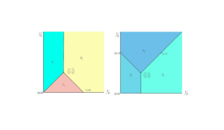
Figure 1: Distribution of $s_{c}$. The left-hand side figure is for $\lambda>1$, the right-hand side figure is for $\lambda\leqslant 1$.

If $\alpha_{1}\geqslant\alpha_{2}$, then

$$R(p,q;\alpha_{1},\alpha_{2})=\begin{cases}n(\alpha_{1}-\alpha_{2})\big{(}\frac{1}{q}-\frac{1}{p}\big{)},\quad&\big{(}\frac{1}{p},\frac{1}{q}\big{)}\in\mbox{S}_{1};\\ n(\alpha_{1}-\alpha_{2})\big{(}\frac{1}{p}+\frac{1}{q}-1\big{)},\quad&\big{(}\frac{1}{p},\frac{1}{q}\big{)}\in\mbox{S}_{2};\\ 0,\quad&\big{(}\frac{1}{p},\frac{1}{q}\big{)}\in\mbox{S}_{3}.\end{cases}$$ (3.5)

If $\alpha_{1}<\alpha_{2}$, then

$$R(p,q;\alpha_{1},\alpha_{2})=\begin{cases}0,\quad&\big{(}\frac{1}{p},\frac{1}{q}\big{)}\in\mbox{T}_{3};\\ n(\alpha_{1}-\alpha_{2})\big{(}\frac{1}{p}+\frac{1}{q}-1\big{)},\quad&\big{(}\frac{1}{p},\frac{1}{q}\big{)}\in\mbox{T}_{2};\\ n(\alpha_{1}-\alpha_{2})\big{(}\frac{1}{q}-\frac{1}{p}\big{)},\quad&\big{(}\frac{1}{p},\frac{1}{q}\big{)}\in\mbox{T}_{1}.\end{cases}$$ (3.6)

Before describing the dilation property of the $\alpha$-modulation spaces, we introduce some critical powers. Let us write $s_{p}=n(1/(1\wedge p)-1)$ and

$$s_{c}=\begin{cases}R(p,q;1,\alpha),&\quad\lambda>1,\\ -R(p,q;\alpha,1),&\quad\lambda\leqslant 1.\end{cases}$$ (3.7)

Theorem 3.1.

Let $0\leqslant\alpha<1,\lambda>0$ and $s+s_{c}\neq 0$. Then

$$\|f_{\lambda}\|_{M_{p,q}^{s,\alpha}}\lesssim\lambda^{-\frac{n}{p}}\left[(1\vee\lambda)^{s_{p}}\vee\lambda^{s+s_{c}}\right]\|f\|_{M_{p,q}^{s,\alpha}}.$$ (3.8)

holds for all $f\in M_{p,q}^{s,\alpha}$. Conversely, if

$$\|f_{\lambda}\|_{M_{p,q}^{s,\alpha}}\lesssim\lambda^{-\frac{n}{p}}F(\lambda)\|f\|_{M_{p,q}^{s,\alpha}}$$

holds for some $F:\ (0,\infty)\to(0,\infty)$ and all $f\in M_{p,q}^{s,\alpha}$, then $F(\lambda)\gtrsim(1\vee\lambda)^{s_{p}}\vee\lambda^{s+s_{c}}$.

Proof.

(Sufficiency) We denote by $\square_{k,1/\lambda}^{\alpha}$ the pseudo-differential operator with symbol $(\eta_{k}^{\alpha})_{\lambda}$. For every $l\in\mathbb{Z}^{n}$ and $\lambda>0$, we introduce

$$\Lambda(l,\lambda)=\{k\in\mathbb{Z}^{n}:\square_{k,1/\lambda}^{\alpha}\square_{l}^{\alpha}f\neq 0\}.$$ (3.9)

For any $k\in\Lambda(l,\lambda)$, it follows from (1.1b) that $k,l$ and $\lambda$ satisfy

$$\lambda\langle l\rangle^{\frac{\alpha}{1-\alpha}}(l_{j}-C)<\langle k\rangle^{\frac{\alpha}{1-\alpha}}(k_{j}+C);$$ (3.10a)

$$\lambda\langle l\rangle^{\frac{\alpha}{1-\alpha}}(l_{j}+C)>\langle k\rangle^{\frac{\alpha}{1-\alpha}}(k_{j}-C)$$ (3.10b)

with $j=1,2,\cdots,n$. In view of (3.10), one sees that $k\in\Lambda(l,\lambda)$ is equivalent to $l\in\Lambda(k,1/\lambda)$. Moreover, if (3.10) holds, then

$$\langle l\rangle\lesssim 1\vee\lambda^{-(1-\alpha)}\ \ \mbox{if and only if }\ \ \langle k\rangle\lesssim 1\vee\lambda^{1-\alpha}.$$ (3.11)

If $\langle l\rangle\gg 1\vee\lambda^{-(1-\alpha)}$, without loss of generality, we may assume $l$ belongs to some $\mathbb{R}^{n}_{j}$, when $l_{j}>0$, from (3.10a); whereas when $l_{j}<0$, from (3.10b)$\times(-1)$, we see $\langle k\rangle^{\frac{1}{1-\alpha}}\gtrsim\lambda\langle l\rangle^{\frac{1}{1-\alpha}}$. Conversely, for $k\in\Lambda(l,\lambda)\cap\mathbb{R}^{n}_{j}$, also from (3.10), we have $\langle k\rangle^{\frac{1}{1-\alpha}}\lesssim\lambda\langle l\rangle^{\frac{1}{1-\alpha}}$. Thus we have

$$\langle k\rangle\sim\lambda^{1-\alpha}\langle l\rangle.$$ (3.12)

Since the volumes of ${\rm supp}(\eta_{k}^{\alpha})_{\lambda}$ and ${\rm supp}\eta_{l}^{\alpha}$ are $O(\lambda^{-n}\langle k\rangle^{\frac{n\alpha}{1-\alpha}})$ and $O(\langle l\rangle^{\frac{n\alpha}{1-\alpha}})$, respectively, we see that

$$\#\Lambda(l,\lambda)\sim 1\vee\lambda^{n(1-\alpha)}.$$ (3.13)

When $q=1$, from Lemma 2.1, we have

$$\begin{split}\left\|\sum_{k\in\Gamma}\square_{k}^{\alpha}f_{\lambda}\right\|_{M_{p,1}^{s,\alpha}}&=\sum_{k\in\Gamma}\langle k\rangle^{\frac{s}{1-\alpha}}\|\square_{k}^{\alpha}f_{\lambda}\|_{p}\\ &=\sum_{k\in\Gamma}\langle k\rangle^{\frac{s}{1-\alpha}}\|(\square_{k,1/\lambda}^{\alpha}f)(\lambda\cdot)\|_{p}\\ &=\lambda^{-\frac{n}{p}}\sum_{k\in\Gamma}\langle k\rangle^{\frac{s}{1-\alpha}}\|\square_{k,1/\lambda}^{\alpha}f\|_{p}\\ &\leqslant\lambda^{-\frac{n}{p}}\sum_{k\in\Gamma}\langle k\rangle^{\frac{s}{1-\alpha}}\sum_{l\in\Lambda(k,1/\lambda)}\|\square_{k,1/\lambda}^{\alpha}\square_{l}^{\alpha}f\|_{p}.\end{split}$$ (3.14)

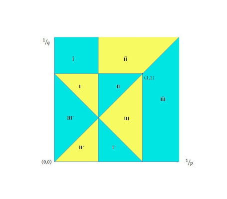
Figure 2: 9 regions for the proof of Theorem 3.1

Case 1. $\bm{\lambda\leqslant 1,\big{(}\frac{1}{p},\frac{1}{q}\big{)}\in\mbox{I}\cup\mbox{II}.}$ For $p=1,\infty$, we apply the same technique as that appeared in Proposition 2.3 to remove $\square_{k,1/\lambda}^{\alpha}$ in (3.14). When $|k|\lesssim 1$, from (3.11) we see that for $l\in\Lambda(k,1/\lambda)$, there is $1\lesssim\langle l\rangle^{\frac{1}{1-\alpha}}\lesssim\frac{1}{\lambda}$, which leads to

$$\begin{split}\left\|\sum_{|k|\lesssim 1}\square_{k}^{\alpha}f_{\lambda}\right\|_{M_{p,1}^{s,\alpha}}&\lesssim\lambda^{-\frac{n}{p}}\sum_{\langle l\rangle\lesssim\lambda^{-(1-\alpha)}}\|\square_{l}^{\alpha}f\|_{p}\lesssim\lambda^{-\frac{n}{p}}\sum_{l\in\mathbb{Z}^{n}}(1\vee\lambda^{s})\langle l\rangle^{\frac{s}{1-\alpha}}\|\square_{l}^{\alpha}f\|_{p}\\ &\lesssim\lambda^{-\frac{n}{p}}(1\vee\lambda^{s})\|f\|_{M_{p,1}^{s,\alpha}}.\end{split}$$ (3.15)

By Plancherel’s identity,

$$\begin{split}\left\|\sum_{|k|\lesssim 1}\square_{k}^{\alpha}f_{\lambda}\right\|_{M_{2,2}^{s,\alpha}}&\lesssim\lambda^{-\frac{n}{2}}\left(\sum_{|k|\lesssim 1}\langle k\rangle^{\frac{2s}{1-\alpha}}\left\|\sum_{l\in\Lambda(k,1/\lambda)}\square_{k,1/\lambda}^{\alpha}\square_{l}^{\alpha}f\right\|_{2}^{2}\right)^{\frac{1}{2}}\\ &\lesssim\lambda^{-\frac{n}{2}}\left(\sum_{\ \langle l\rangle\lesssim\lambda^{-(1-\alpha)}}\|\square_{l}^{\alpha}f\|_{2}^{2}\right)^{\frac{1}{2}}\lesssim\lambda^{-\frac{n}{2}}(1\vee\lambda^{s})\|f\|_{M_{2,2}^{s,\alpha}}.\end{split}$$ (3.16)

When $|k|\gg 1$, from (3.12)-(3.14), we see that

$$\begin{split}\left\|\sum_{|k|\gg 1}\square_{k}^{\alpha}f_{\lambda}\right\|_{M_{p,1}^{s,\alpha}}&\lesssim\lambda^{-\frac{n}{p}+s}\sum_{|k|\gg 1}\sum_{l\in\Lambda(k,1/\lambda)}\langle l\rangle^{\frac{s}{1-\alpha}}\|\square_{l}^{\alpha}f\|_{p}\\ &\lesssim\lambda^{-\frac{n}{p}+s}\sum_{l}\langle l\rangle^{\frac{s}{1-\alpha}}\sum_{k\in\Lambda(l,\lambda)}\|\square_{l}^{\alpha}f\|_{p}\lesssim\lambda^{-\frac{n}{p}+s}\|f\|_{M_{p,1}^{s,\alpha}}.\end{split}$$ (3.17)

In view of Plancherel’s formula,

$$\begin{split}\left\|\sum_{|k|\gg 1}\square_{k}^{\alpha}f_{\lambda}\right\|_{M_{2,2}^{s,\alpha}}&\leqslant\lambda^{-\frac{n}{2}+s}\left(\sum_{|k|\gg 1}\sum_{l\in\Lambda(k,1/\lambda)}\langle l\rangle^{\frac{2s}{1-\alpha}}\|\square_{k,1/\lambda}^{\alpha}\square_{l}^{\alpha}f\|_{2}^{2}\right)^{\frac{1}{2}}\\ &\lesssim\lambda^{-\frac{n}{2}+s}\left(\sum_{l}\langle l\rangle^{\frac{2s}{1-\alpha}}\sum_{k\in\Lambda(l,\lambda)}\|\square_{k,1/\lambda}^{\alpha}\square_{l}^{\alpha}f\|_{2}^{2}\right)^{\frac{1}{2}}\lesssim\lambda^{-\frac{n}{2}+s}\|f\|_{M_{2,2}^{s,\alpha}}.\end{split}$$ (3.18)

Combining (3.15)-(3.18), we use complex interpolation to get

$$\|f_{\lambda}\|_{M_{p,q}^{s,\alpha}}\lesssim\lambda^{-\frac{n}{p}}(1\vee\lambda^{s})\|f\|_{M_{p,q}^{s,\alpha}}.$$ (3.19)

Case 2. $\bm{\lambda>1,\big{(}\frac{1}{p},\frac{1}{q}\big{)}\in\mbox{I}\cup\mbox{III}^{*}.}$ Through the point $\big{(}\frac{1}{p},\frac{1}{q}\big{)}$, one can draw the parallel line to the $\frac{1}{q}$-axis. We assume there exists some $(\theta,\eta)\in[0,1]\times[0,1]$, such that the parallel line cuts the line segment connecting $(0,1),\big{(}\frac{1}{2},1\big{)}$ and the line segment connecting $(0,0),\big{(}\frac{1}{2},\frac{1}{2}\big{)}$ at $\big{(}\frac{\theta}{2},1\big{)}$ and $\big{(}\frac{\theta}{2},\frac{\theta}{2}\big{)}$, respectively. Assume that

$$\frac{1}{p}=\frac{\theta}{2},\quad\frac{1}{q}=1-\left(1-\frac{\theta}{2}\right)\eta.$$

When $|k|\lesssim\lambda^{1-\alpha}$, from (3.11) and (3.14), we have

$$\begin{split}\left\|\sum_{|k|\lesssim\lambda^{1-\alpha}}\square_{k}^{\alpha}f_{\lambda}\right\|_{M_{\infty,1}^{s,\alpha}}&\leqslant\sum_{|l|\lesssim 1}\|\square_{l}^{\alpha}f\|_{\infty}\sum_{k\in\Lambda(l,\lambda)}\langle k\rangle^{\frac{s}{1-\alpha}}\lesssim\Big{(}1\vee\lambda^{s+n(1-\alpha)}\Big{)}\|f\|_{M_{\infty,1}^{s,\alpha}}.\end{split}$$ (3.20)

By the Schwartz inequality and the Plancherel identity,

$$\begin{split}\left\|\sum_{|k|\lesssim\lambda^{1-\alpha}}\square_{k}^{\alpha}f_{\lambda}\right\|_{M_{2,1}^{s,\alpha}}&\leqslant\lambda^{-\frac{n}{2}}\sum_{|l|\lesssim 1}\left(\sum_{k\in\Lambda(l,\lambda)}\|\square_{k,1/\lambda}^{\alpha}\square_{l}^{\alpha}f\|_{2}^{2}\right)^{\frac{1}{2}}\left(\sum_{k\in\Lambda(l,\lambda)}\langle k\rangle^{\frac{2s}{1-\alpha}}\right)^{\frac{1}{2}}\\ &\lesssim\lambda^{-\frac{n}{2}}\Big{(}1\vee\lambda^{s+\frac{n}{2}(1-\alpha)}\Big{)}\|f\|_{M_{2,1}^{s,\alpha}}.\end{split}$$ (3.21)

From (3.11), we have

$$\begin{split}\left\|\sum_{|k|\lesssim\lambda^{1-\alpha}}\square_{k}^{\alpha}f_{\lambda}\right\|_{M_{\infty,\infty}^{s,\alpha}}&\lesssim\sup_{|k|\lesssim\lambda^{1-\alpha}}\langle k\rangle^{\frac{s}{1-\alpha}}\|\square_{k}^{\alpha}f_{\lambda}\|_{\infty}\\ &\lesssim(1\vee\lambda^{s})\sup_{|k|\lesssim\lambda^{1-\alpha}}\sum_{l\in\Lambda(k,1/\lambda)}\|\square_{k,1/\lambda}^{\alpha}\square_{l}^{\alpha}f\|_{\infty}\\ &\lesssim(1\vee\lambda^{s})\sup_{|l|\lesssim 1}\|\square_{l}^{\alpha}f\|_{\infty}\lesssim(1\vee\lambda^{s})\|f\|_{M_{\infty,\infty}^{s,\alpha}}.\end{split}$$ (3.22)

In view of Plancherel’s equality,

$$\begin{split}\left\|\sum_{|k|\lesssim\lambda^{1-\alpha}}\square_{k}^{\alpha}f_{\lambda}\right\|_{M_{2,2}^{s,\alpha}}&\lesssim\left(\sum_{|k|\lesssim\lambda^{1-\alpha}}\langle k\rangle^{\frac{2s}{1-\alpha}}\|\square_{k}^{\alpha}f_{\lambda}\|_{2}^{2}\right)^{\frac{1}{2}}\\ &\lesssim\lambda^{-\frac{n}{2}}\left(\sum_{|l|\lesssim 1}(1\vee\lambda^{s})^{2}\sum_{k\in\Lambda(l,\lambda)}\|\square_{k,1/\lambda}^{\alpha}\square_{l}^{\alpha}f\|_{2}^{2}\right)^{\frac{1}{2}}\\ &\lesssim\lambda^{-\frac{n}{2}}(1\vee\lambda^{s})\left(\sum_{|l|\lesssim 1}\|\square_{l}^{\alpha}f\|_{2}^{2}\right)^{\frac{1}{2}}\lesssim\lambda^{-\frac{n}{2}}(1\vee\lambda^{s})\|f\|_{M_{2,2}^{s,\alpha}}.\end{split}$$ (3.23)

When $|k|\gg\lambda^{1-\alpha}$, from (3.12)-(3.14), we have

$$\begin{split}\left\|\sum_{|k|\gg\lambda^{1-\alpha}}\square_{k}^{\alpha}f_{\lambda}\right\|_{M_{\infty,1}^{s,\alpha}}&\leqslant\lambda^{s}\sum_{|l|\gg 1}\langle l\rangle^{\frac{s}{1-\alpha}}\sum_{k\in\Lambda(l,\lambda)}\|\square_{l}^{\alpha}f\|_{\infty}\lesssim\lambda^{s+n(1-\alpha)}\|f\|_{M_{\infty,1}^{s,\alpha}}.\end{split}$$ (3.24)

By Jensen’s inequality,

$$\begin{split}\left\|\sum_{|k|\gg\lambda^{1-\alpha}}\square_{k}^{\alpha}f_{\lambda}\right\|_{M_{2,1}^{s,\alpha}}&\lesssim\lambda^{-\frac{n}{2}+s}\sum_{|l|\gg 1}\langle l\rangle^{\frac{s}{1-\alpha}}\sum_{k\in\Lambda(l,\lambda)}\|\square_{k,1/\lambda}^{\alpha}\square_{l}^{\alpha}f\|_{2}\\ &\lesssim\lambda^{\frac{n}{2}+s}\sum_{|l|\gg 1}\langle l\rangle^{\frac{s}{1-\alpha}}[\#\Lambda(l,\lambda)]^{\frac{1}{2}}\left(\sum_{k\in\Lambda(l,\lambda)}\|\square_{k,1/\lambda}^{\alpha}\square_{l}^{\alpha}f\|_{2}^{2}\right)^{\frac{1}{2}}\\ &\lesssim\lambda^{-\frac{n}{2}+s+\frac{n}{2}(1-\alpha)}\|f\|_{M_{2,1}^{s,\alpha}}.\end{split}$$ (3.25)

From (3.12),(3.13), we have

$$\begin{split}\left\|\sum_{|k|\gg\lambda^{1-\alpha}}\square_{k}^{\alpha}f_{\lambda}\right\|_{M_{\infty,\infty}^{s,\alpha}}&\lesssim\sup_{k}\langle k\rangle^{\frac{s}{1-\alpha}}\|\square_{k,1/\lambda}^{\alpha}f\|_{\infty}\\ &\lesssim\lambda^{s}\sup_{k}\sum_{l\in\Lambda(k,1/\lambda)}\langle l\rangle^{\frac{s}{1-\alpha}}\|\square_{k,1/\lambda}^{\alpha}\square_{l}^{\alpha}f\|_{\infty}\lesssim\lambda^{s}\|f\|_{M_{\infty,\infty}^{s,\alpha}}.\end{split}$$ (3.26)

Similar to (3.18), one has that

$$\left\|\sum_{|k|\gg\lambda^{1-\alpha}}\square_{k}^{\alpha}f_{\lambda}\right\|_{M_{2,2}^{s,\alpha}}\lesssim\lambda^{-\frac{n}{2}+s}\|f\|_{M_{2,2}^{s,\alpha}}.$$ (3.27)

Since $n(1-\alpha)\big{(}1-\frac{\theta}{2}\big{)}=(1-\theta)n(1-\alpha)+\theta\frac{n}{2}(1-\alpha)$, combining (3.20),(3.24),(3.21),(3.25), complex interpolation yields

$$\|f_{\lambda}\|_{M_{\frac{2}{\theta},1}^{s,\alpha}}\lesssim\lambda^{-\frac{\theta}{2}n}\left(1\vee\lambda^{s+n(1-\alpha)\big{(}1-\frac{\theta}{2}\big{)}}\right)\|f\|_{M_{\frac{2}{\theta},1}^{s,\alpha}}.$$ (3.28)

Combining (3.22),(3.26),(3.23),(3.27), complex interpolation yields

$$\|f_{\lambda}\|_{M_{\frac{2}{\theta},\frac{2}{\theta}}^{s,\alpha}}\lesssim\lambda^{-\frac{\theta}{2}n}(1\vee\lambda^{s})\|f\|_{M_{\frac{2}{\theta},\frac{2}{\theta}}^{s,\alpha}}.$$ (3.29)

Interpolating (3.28) and (3.29), we have

$$\|f_{\lambda}\|_{M_{p,q}^{s,\alpha}}\lesssim\lambda^{-\frac{n}{p}}\left(1\vee\lambda^{s+n(1-\alpha)\big{(}\frac{1}{q}-\frac{1}{p}\big{)}}\right)\|f\|_{M_{p,q}^{s,\alpha}}.$$ (3.30)

Case 3. $\bm{\lambda>1,\big{(}\frac{1}{p},\frac{1}{q}\big{)}\in\mbox{II}\cup\mbox{III}.}$ Through the point $\big{(}\frac{1}{p},\frac{1}{q}\big{)}$ one can make the parallel line to the $\frac{1}{q}$-axis. We assume there exists some $(\theta,\eta)\in[0,1]\times[0,1]$, such that the parallel line cuts the line segment connecting $(1,1),\big{(}\frac{1}{2},1\big{)}$ and the line segment connecting $(1,0),\big{(}\frac{1}{2},\frac{1}{2}\big{)}$ at $\big{(}1-\frac{\theta}{2},1\big{)}$ and $\big{(}1-\frac{\theta}{2},\frac{\theta}{2}\big{)}$, respectively. We can assume that

$$\frac{1}{p}=1-\frac{\theta}{2},\quad\frac{1}{q}=1-\left(1-\frac{\theta}{2}\right)\eta.$$

When $|k|\lesssim\lambda^{1-\alpha}$, similarly to (3.20) and (3.22), we have

$$\left\|\sum_{|k|\lesssim\lambda^{1-\alpha}}\square_{k}^{\alpha}f_{\lambda}\right\|_{M_{1,1}^{s,\alpha}}\lesssim\lambda^{-n}\left(1\vee\lambda^{s+n(1-\alpha)}\right)\|f\|_{M_{1,1}^{s,\alpha}};$$ (3.31)

$$\left\|\sum_{|k|\lesssim\lambda^{1-\alpha}}\square_{k}^{\alpha}f_{\lambda}\right\|_{M_{1,\infty}^{s,\alpha}}\lesssim\lambda^{-n}\left(1\vee\lambda^{s}\right)\|f\|_{M_{1,\infty}^{s,\alpha}}.$$ (3.32)

When $|k|\gg\lambda^{1-\alpha}$, similarly to (3.24) and (3.26), we have

$$\left\|\sum_{|k|\gg\lambda^{1-\alpha}}\square_{k}^{\alpha}f_{\lambda}\right\|_{M_{1,1}^{s,\alpha}}\lesssim\lambda^{-n+s+n(1-\alpha)}\|f\|_{M_{1,1}^{s,\alpha}};$$ (3.33)

$$\left\|\sum_{|k|\gg\lambda^{1-\alpha}}\square_{k}^{\alpha}f_{\lambda}\right\|_{M_{1,\infty}^{s,\alpha}}\lesssim\lambda^{-n+s}\|f\|_{M_{1,\infty}^{s,\alpha}}.$$ (3.34)

Combining (3.31),(3.33),(3.21),(3.25), complex interpolation yields

$$\|f_{\lambda}\|_{M_{\frac{2}{2-\theta},1}^{s,\alpha}}\lesssim\lambda^{-\frac{n}{2}\big{(}1-\frac{\theta}{2}\big{)}}\left(1\vee\lambda^{s+n(1-\alpha)\big{(}1-\frac{\theta}{2}\big{)}}\right)\|f\|_{M_{\frac{2}{2-\theta},1}^{s,\alpha}}.$$ (3.35)

Combining (3.32),(3.34),(3.23),(3.27), complex interpolation yields

$$\|f_{\lambda}\|_{M_{\frac{2}{2-\theta},\frac{2}{\theta}}^{s,\alpha}}\lesssim\lambda^{-\frac{n}{2}\big{(}1-\frac{\theta}{2}\big{)}}\left(1\vee\lambda^{s}\right)\|f\|_{M_{\frac{2}{2-\theta},\frac{2}{\theta}}^{s,\alpha}}.$$ (3.36)

Interpolating (3.35) and (3.36), we have

$$\|f_{\lambda}\|_{M_{p,q}^{s,\alpha}}\lesssim\lambda^{-\frac{n}{p}}\left(1\vee\lambda^{s+n(1-\alpha)\big{(}\frac{1}{p}+\frac{1}{q}-1\big{)}}\right)\|f\|_{M_{p,q}^{s,\alpha}}.$$ (3.37)

Case 4. $\bm{\lambda\leqslant 1,\big{(}\frac{1}{p},\frac{1}{q}\big{)}\in\{\mbox{I}^{*}\cup\mbox{II}^{*}\cup\mbox{III}\cup\mbox{III}^{*}\}\backslash\{(0,1]\times[0,1]\}};\,{\bf or}\,\bm{\lambda>1,\big{(}\frac{1}{p},\frac{1}{q}\big{)}}$ $\bm{\in\mbox{I}^{*}\cup\mbox{II}^{*}\backslash\{(1,0)\}.}$ We observe that, for any $\big{(}\frac{1}{p},\frac{1}{q}\big{)}\in\mbox{I}^{\ast}\cup\mbox{II}^{\ast}$, we have $\big{(}\frac{1}{p^{*}},\frac{1}{q^{*}}\big{)}\in\mbox{I}\cup\mbox{II}$. By duality,

$$\begin{split}|\langle f_{\lambda},g\rangle|=\frac{1}{\lambda^{n}}|\langle f,g_{\frac{1}{\lambda}}\rangle|\leqslant\frac{1}{\lambda^{n}}\|f\|_{M_{p,q}^{s,\alpha}}\big{\|}g_{\frac{1}{\lambda}}\big{\|}_{M_{p^{\ast},q^{\ast}}^{-s,\alpha}}.\end{split}$$ (3.38)

If we denote $\|f_{\lambda}\|_{M_{p,q}^{s,\alpha}}\lesssim F(s,\lambda;p,q)\|f\|_{M_{p,q}^{s,\alpha}}$, from the previous several cases, we know that

$$\begin{split}\big{\|}g_{\frac{1}{\lambda}}\big{\|}_{M_{p^{\ast},q^{\ast}}^{-s,\alpha}}\lesssim F\left(-s,\lambda^{-1};p^{*},q^{*}\right)\|g\|_{M_{p^{\ast},q^{\ast}}^{-s,\alpha}}.\end{split}$$ (3.39)

By the principle of duality, it follows from (3.38) and (3.39) that

$$\begin{split}\|f_{\lambda}\|_{M_{p,q}^{s,\alpha}}&\lesssim\lambda^{-n}F\left(-s,\lambda^{-1};p^{*},q^{*}\right)\|f\|_{M_{p,q}^{s,\alpha}}.\end{split}$$ (3.40)

For $\lambda\leqslant 1$ with $\big{(}\frac{1}{p},\frac{1}{q}\big{)}\in\{\mbox{I}^{*}\cup\mbox{III}\}\backslash\{1\}\times[0,1]$, from Case 2, (3.40) gives

$$\|f_{\lambda}\|_{M_{p,q}^{s,\alpha}}\lesssim\lambda^{-\frac{n}{p}}\left(1\vee\lambda^{s-n(1-\alpha)\big{(}\frac{1}{p}-\frac{1}{q}\big{)}}\right)\|f\|_{M_{p,q}^{s,\alpha}}.$$ (3.41)

For $\lambda\leqslant 1$ with $\big{(}\frac{1}{p},\frac{1}{q}\big{)}\in\{\mbox{II}^{*}\cup\mbox{III}^{*}\}\backslash\{(0,1)\}$, from Case 3, (3.40) gives

$$\|f_{\lambda}\|_{M_{p,q}^{s,\alpha}}\lesssim\lambda^{-\frac{n}{p}}\left(1\vee\lambda^{s-n(1-\alpha)\big{(}1-\frac{1}{q}-\frac{1}{p}\big{)}}\right)\|f\|_{M_{p,q}^{s,\alpha}}.$$ (3.42)

For $\lambda>1$ with $\big{(}\frac{1}{p},\frac{1}{q}\big{)}\in\mbox{I}^{*}\cup\mbox{II}^{*}\backslash\{(1,0)\}$, from Case 1, (3.40) gives

$$\|f_{\lambda}\|_{M_{p,q}^{s,\alpha}}\lesssim\lambda^{-\frac{n}{p}}(1\vee\lambda^{s})\|f\|_{M_{p,q}^{s,\alpha}}.$$ (3.43)

Case 5. $\bm{\big{(}\frac{1}{p},\frac{1}{q}\big{)}\in\{\widehat{\mbox{I}}\cup\widehat{\mbox{II}}\}\backslash(1,\infty)\times(1,\infty).}$ Since $\ell^{q}\subset\ell^{1}$, we know

$$\begin{split}\|\square_{k}^{\alpha}f_{\lambda}\|_{p}\lesssim\lambda^{-\frac{n}{p}}\sum_{l\in\Lambda(k,1/\lambda)}\|\square_{k,1/\lambda}^{\alpha}\square_{l}^{\alpha}f\|_{p}\lesssim\lambda^{-\frac{n}{p}}\left(\sum_{l\in\Lambda(k,1/\lambda)}\|\square_{k,1/\lambda}^{\alpha}\square_{l}^{\alpha}f\|_{p}^{q}\right)^{\frac{1}{q}}.\end{split}$$ (3.44)

From (3.44),(3.11), when $\lambda\leqslant 1$ and $|k|\lesssim 1$, we conclude that

$$\begin{split}\left\|\sum_{|k|\lesssim 1}\square_{k}^{\alpha}f_{\lambda}\right\|_{M_{\infty,q}^{s,\alpha}}&\lesssim\left(\sum_{|k|\lesssim 1}\langle k\rangle^{\frac{sq}{1-\alpha}}\|\square_{k}^{\alpha}f_{\lambda}\|_{\infty}^{q}\right)^{\frac{1}{q}}\\ &\lesssim\left(\sum_{|k|\lesssim 1}\langle k\rangle^{\frac{sq}{1-\alpha}}\sum_{l\in\Lambda(k,1/\lambda)}\|\square_{k,1/\lambda}^{\alpha}\square_{l}^{\alpha}f\|_{\infty}^{q}\right)^{\frac{1}{q}}\\ &\lesssim\left(\sum_{\langle l\rangle\lesssim\lambda^{-(1-\alpha)}}\|\square_{l}^{\alpha}f\|_{\infty}^{q}\right)^{\frac{1}{q}}\lesssim(1\vee\lambda^{s})\|f\|_{M_{\infty,q}^{s,\alpha}};\end{split}$$ (3.45)

and when $\lambda>1$ and $|k|\lesssim\lambda^{1-\alpha}$,

$$\begin{split}\left\|\sum_{|k|\lesssim\lambda^{1-\alpha}}\square_{k}^{\alpha}f_{\lambda}\right\|_{M_{\infty,q}^{s,\alpha}}&\lesssim\left(\sum_{|k|\lesssim\lambda^{1-\alpha}}\langle k\rangle^{\frac{sq}{1-\alpha}}\|\square_{k}^{\alpha}f_{\lambda}\|_{\infty}^{q}\right)^{\frac{1}{q}}\\ &\lesssim\left(\sum_{|k|\lesssim\lambda^{1-\alpha}}\langle k\rangle^{\frac{sq}{1-\alpha}}\sum_{l\in\Lambda(k,1/\lambda)}\|\square_{l}^{\alpha}f\|_{\infty}^{q}\right)^{\frac{1}{q}}\\ &\lesssim\left(\sum_{|l|\lesssim 1}\|\square_{l}^{\alpha}f\|_{\infty}^{q}\sum_{|k|\lesssim\lambda^{1-\alpha}}\langle k\rangle^{\frac{sq}{1-\alpha}}\right)^{\frac{1}{q}}\\ &\lesssim\left(1\vee\lambda^{s+n(1-\alpha)\frac{1}{q}}\right)\|f\|_{M_{\infty,q}^{s,\alpha}}.\end{split}$$ (3.46)

When $|k|\gg 1\vee\lambda^{1-\alpha}$, from (3.44), (3.12), (3.13), we have

$$\begin{split}\left\|\sum_{|k|\gg 1\vee\lambda^{1-\alpha}}\square_{k}^{\alpha}f_{\lambda}\right\|_{M_{\infty,q}^{s,\alpha}}&\lesssim\left(\sum_{|k|\gg 1\vee\lambda^{1-\alpha}}\langle k\rangle^{\frac{sq}{1-\alpha}}\sum_{l\in\Lambda(k,1/\lambda)}\|\square_{l}^{\alpha}f\|_{\infty}^{q}\right)^{\frac{1}{q}}\\ &\lesssim\lambda^{s}\left(\sum_{|l|\gg 1}\langle l\rangle^{\frac{sq}{1-\alpha}}\sum_{k\in\Lambda(l,\lambda)}\|\square_{l}^{\alpha}f\|_{\infty}\right)^{\frac{1}{q}}\\ &\lesssim\lambda^{s}(1\vee\lambda)^{n(1-\alpha)\frac{1}{q}}\|f\|_{M_{\infty,q}^{s,\alpha}}.\end{split}$$ (3.47)

Therefore, combining (3.45)-(3.47), we get

$$\|f_{\lambda}\|_{M_{\infty,q}^{s,\alpha}}\lesssim 1\vee\lambda^{s}\vee\lambda^{s+n(1-\alpha)\frac{1}{q}}\|f\|_{M_{\infty,q}^{s,\alpha}}.$$ (3.48)

The same for $M_{1,q}^{s,\alpha}$. Corresponding to (3.48), we get

$$\|f_{\lambda}\|_{M_{1,q}^{s,\alpha}}\lesssim\lambda^{-n}\left(1\vee\lambda^{s}\vee\lambda^{s+n(1-\alpha)\frac{1}{q}}\right)\|f\|_{M_{1,q}^{s,\alpha}}.$$ (3.49)

Whereas when $p=2,\lambda\leqslant 1$ and $|k|\lesssim 1$, from (3.44),(3.11), we have

$$\begin{split}\left\|\sum_{|k|\lesssim 1}\square_{k}^{\alpha}f_{\lambda}\right\|_{M_{2,q}^{s,\alpha}}&\lesssim\lambda^{-\frac{n}{2}}\left(\sum_{|k|\lesssim 1}\langle k\rangle^{\frac{sq}{1-\alpha}}\sum_{l\in\Lambda(k,1/\lambda)}\|\square_{k,1/\lambda}^{\alpha}\square_{l}^{\lambda}f\|_{2}^{q}\right)^{\frac{1}{q}}\\ &\lesssim\lambda^{-\frac{n}{2}}\left(\sum_{\langle l\rangle\lesssim\lambda^{-(1-\alpha)}}\|\square_{l}^{\alpha}f\|_{2}^{q}\right)^{\frac{1}{q}}\lesssim\lambda^{-\frac{n}{2}}(1\vee\lambda^{s})\|f\|_{M_{2,q}^{s,\alpha}}.\end{split}$$ (3.50)

When $\lambda>1,|k|\lesssim\lambda^{1-\alpha}$, by (3.44), (3.11) and Hölder’s inequality, we have

$$\begin{split}\left\|\sum_{|k|\lesssim\lambda^{1-\alpha}}\square_{k}^{\alpha}f_{\lambda}\right\|_{M_{2,q}^{s,\alpha}}&\lesssim\lambda^{-\frac{n}{2}}\left(\sum_{|l|\lesssim 1}\sum_{k\in\Lambda(l,\lambda)}\langle k\rangle^{\frac{sq}{1-\alpha}}\|\square_{k,1/\lambda}^{\alpha}\square_{l}^{\alpha}f\|_{2}^{q}\right)^{\frac{1}{q}}\\ &\lesssim\lambda^{-\frac{n}{2}}\left[\sum_{|l|\lesssim 1}\left(\sum_{k\in\Lambda(l,\lambda)}\|\square_{k,1/\lambda}^{\alpha}\square_{l}^{\alpha}f\|_{2}^{2}\right)^{\frac{q}{2}}\left(\sum_{|k|\lesssim\lambda^{1-\alpha}}\langle k\rangle^{\frac{sq}{1-\alpha}\cdot\frac{2}{2-q}}\right)^{\frac{2-q}{2}}\right]^{\frac{1}{q}}\\ &\lesssim\lambda^{-\frac{n}{2}}\left(1\vee\lambda^{s+n(1-\alpha)\big{(}\frac{1}{q}-\frac{1}{2}\big{)}}\right)\|f\|_{M_{2,q}^{s,\alpha}}.\end{split}$$ (3.51)

When $|k|\gg 1\vee\lambda^{1-\alpha}$, in view of (3.44),(3.12),(3.13) and Hölder’s inequality, we have

$$\begin{split}\left\|\sum_{|k|\gg 1\vee\lambda^{1-\alpha}}\square_{k}^{\alpha}f_{\lambda}\right\|_{M_{2,q}^{s,\alpha}}&\lesssim\lambda^{-\frac{n}{2}+s}\left(\sum_{|l|\gg 1}\langle l\rangle^{\frac{sq}{1-\alpha}}\sum_{k\in\Lambda(l,\lambda)}\|\square_{l}^{\alpha}\square_{k,1/\lambda}^{\alpha}f\|_{2}^{q}\right)^{\frac{1}{q}}\\ &\lesssim\lambda^{-\frac{n}{2}+s}\left[\sum_{|l|\gg 1}\langle l\rangle^{\frac{sq}{1-\alpha}}[\#\Lambda(l,\lambda)]^{1-\frac{q}{2}}\left(\sum_{k\in\Lambda(l,\lambda)}\|\square_{l}^{\alpha}\square_{k,1/\lambda}^{\alpha}f\|_{2}^{2}\right)^{\frac{q}{2}}\right]^{\frac{1}{q}}\\ &\lesssim\lambda^{-\frac{n}{2}+s}(1\vee\lambda)^{n(1-\alpha)\big{(}\frac{1}{q}-\frac{1}{2}\big{)}}\|f\|_{M_{2,q}^{s,\alpha}}.\end{split}$$ (3.52)

Therefore, combining (3.50)-(3.52), we get

$$\|f_{\lambda}\|_{M_{2,q}^{s,\alpha}}\lesssim\lambda^{-\frac{n}{2}}\left(1\vee\lambda^{s}\vee\lambda^{s+n(1-\alpha)\big{(}\frac{1}{q}-\frac{1}{2}\big{)}}\right)\|f\|_{M_{2,q}^{s,\alpha}}.$$ (3.53)

For $\big{(}\frac{1}{p},\frac{1}{q}\big{)}\in\widehat{\mbox{I}}$, complex interpolation between (3.48) and (3.53) yields

$$\|f_{\lambda}\|_{M_{p,q}^{s,\alpha}}\lesssim\lambda^{-\frac{n}{p}}\left(1\vee\lambda^{s}\vee\lambda^{s+n(1-\alpha)\big{(}\frac{1}{q}-\frac{1}{p}\big{)}}\right)\|f\|_{M_{p,q}^{s,\alpha}};$$ (3.54)

while for $\big{(}\frac{1}{p},\frac{1}{q}\big{)}\in\widehat{\mbox{II}}\backslash(1,\infty)\times(1,\infty)$, complex interpolation between (3.49) and (3.53) yields

$$\|f_{\lambda}\|_{M_{p,q}^{s,\alpha}}\lesssim\lambda^{-\frac{n}{p}}\left(1\vee\lambda^{s}\vee\lambda^{s+n(1-\alpha)\big{(}\frac{1}{p}+\frac{1}{q}-1\big{)}}\right)\|f\|_{M_{p,q}^{s,\alpha}}.$$ (3.55)

Case 6.  $\bm{\big{(}\frac{1}{p},\frac{1}{q}\big{)}\in\widehat{\mbox{III}}.}$ Since $l^{p}\subset l^{1}$, we know

$$\begin{split}\|\square_{k}^{\alpha}f_{\lambda}\|_{p}=\lambda^{-\frac{n}{p}}\|\square_{k,1/\lambda}^{\alpha}f\|_{p}\leqslant\lambda^{-\frac{n}{p}}\left(\sum_{l\in\Lambda(k,1/\lambda)}\|\square_{k,1/\lambda}^{\alpha}\square_{l}^{\alpha}f\|_{p}^{p}\right)^{\frac{1}{p}}.\end{split}$$ (3.56)

When $\lambda\leqslant 1$ and $|k|\lesssim 1$, from (1.1b),(3.12), we see that

$$\mbox{diam}\;\mbox{supp}\mathscr{F}[(\mathscr{F}^{-1}(\eta_{k}^{\alpha})_{\lambda})(x-\cdot)\square_{l}^{\alpha}f(\cdot)]\lesssim 1/\lambda,$$

By Proposition 2.1, imitating the processes as in (LABEL:equivalent-ffdfddfdfdfdfd)-(LABEL:algebra-p<1-2), we get

$$\|\square_{k,1/\lambda}^{\alpha}\square_{l}^{\alpha}f\|_{p}\lesssim\left(1/\lambda\right)^{n\big{(}\frac{1}{p}-1\big{)}}\left(\lambda\big{/}\langle k\rangle^{\frac{\alpha}{1-\alpha}}\right)^{n\big{(}\frac{1}{p}-1\big{)}}\|\square_{l}^{\alpha}f\|_{p}\lesssim\|\square_{l}^{\alpha}f\|_{p}.$$ (3.57)

From (3.56), (3.57), the embedding $\ell^{1}\subset\ell^{\frac{q}{p}}$, and Hölder’s inequality, we have

$$\begin{split}\left\|\sum_{|k|\lesssim 1}\square_{k}^{\alpha}f_{\lambda}\right\|_{M_{p,q}^{s,\alpha}}&\lesssim\lambda^{-\frac{n}{p}}\left[\sum_{|k|\lesssim 1}\langle k\rangle^{\frac{sq}{1-\alpha}}\left(\sum_{l\in\Lambda(k,1/\lambda)}\|\square_{k,1/\lambda}^{\alpha}\square_{l}^{\alpha}f\|_{p}^{p}\right)^{\frac{q}{p}}\right]^{\frac{1}{q}}\\ &\lesssim\lambda^{-\frac{n}{p}}\left(\sum_{|k|\lesssim 1}\langle k\rangle^{\frac{sp}{1-\alpha}}\sum_{l\in\Lambda(k,1/\lambda)}\|\square_{k,1/\lambda}^{\alpha}\square_{l}^{\alpha}f\|_{p}^{p}\right)^{\frac{1}{p}}\\ &\lesssim\lambda^{-\frac{n}{p}}\left[\sum_{\langle l\rangle\lesssim\lambda^{-(1-\alpha)}}\left(\sum_{|k|\lesssim 1}\langle k\rangle^{\frac{s}{1-\alpha}\cdot\frac{pq}{q-p}}\right)^{\frac{q-p}{q}}\left(\sum_{|k|\lesssim 1}\|\square_{l}^{\alpha}f\|_{p}^{q}\right)^{\frac{p}{q}}\right]^{\frac{1}{p}}\\ &\lesssim\lambda^{-\frac{n}{p}}(1\vee\lambda^{s})\|f\|_{M_{p,q}^{s,\alpha}}.\end{split}$$ (3.58)

When $\lambda\leqslant 1$ and $|k|\gg 1$, from (1.1b), (3.12), we see that

$$\mbox{diam}\;\mbox{supp}\mathscr{F}[(\mathscr{F}^{-1}(\eta_{k}^{\alpha})_{\lambda})(x-\cdot)\square_{l}^{\alpha}f(\cdot)]\lesssim\langle k\rangle^{\frac{\alpha}{1-\alpha}}/\lambda.$$

Similarly to (3.57), we get

$$\|\square_{k,1/\lambda}^{\alpha}\square_{l}^{\alpha}f\|_{p}\lesssim\left(\langle k\rangle^{\frac{\alpha}{1-\alpha}}/\lambda\right)^{n\big{(}\frac{1}{p}-1\big{)}}\left(\lambda\big{/}\langle k\rangle^{\frac{\alpha}{1-\alpha}}\right)^{n\big{(}\frac{1}{p}-1\big{)}}\|\square_{l}^{\alpha}f\|_{p}\leqslant\|\square_{l}^{\alpha}f\|_{p}.$$ (3.59)

From (3.56), (3.59), (3.12), (3.13), we have

$$\begin{split}\left\|\sum_{|k|\gg 1}\square_{k}^{\alpha}f_{\lambda}\right\|_{M_{p,q}^{s,\alpha}}&\lesssim\lambda^{-\frac{n}{p}}\left[\sum_{|k|\gg 1}\langle k\rangle^{\frac{sq}{1-\alpha}}\left(\sum_{l\in\Lambda(k,1/\lambda)}\|\square_{k,1/\lambda}^{\alpha}\square_{l}^{\alpha}f\|_{p}^{p}\right)^{\frac{q}{p}}\right]^{\frac{1}{q}}\\ &\lesssim\lambda^{-\frac{n}{p}+s}\left(\sum_{|k|\gg 1}[\#\Lambda(k,1/\lambda)]^{\frac{q}{p}-1}\sum_{l\in\Lambda(k,1/\lambda)}\langle l\rangle^{\frac{sq}{1-\alpha}}\|\square_{l}^{\alpha}f\|_{p}^{q}\right)^{\frac{1}{q}}\\ &\lesssim\lambda^{-\frac{n}{p}+s-n(1-\alpha)\big{(}\frac{1}{p}-\frac{1}{q}\big{)}}\left(\sum_{l}\langle l\rangle^{\frac{sq}{1-\alpha}}\sum_{k\in\Lambda(l,\lambda)}\|\square_{l}^{\alpha}f\|_{p}^{q}\right)^{\frac{1}{q}}\\ &\lesssim\lambda^{-\frac{n}{p}+s-n(1-\alpha)\big{(}\frac{1}{p}-\frac{1}{q}\big{)}}\|f\|_{M_{p,q}^{s,\alpha}}.\end{split}$$ (3.60)

For $\lambda>1$ and $|k|\lesssim\lambda^{1-\alpha}$, from (1.1b), (3.12), we know

$$\mbox{diam}\;\mbox{supp}\mathscr{F}[(\mathscr{F}^{-1}(\eta_{k}^{\alpha})_{\lambda})(x-\cdot)\square_{l}^{\alpha}f(\cdot)]\lesssim 1.$$

Similarly to (3.57), we get

$$\|\square_{k,1/\lambda}^{\alpha}\square_{l}^{\alpha}f\|_{p}\lesssim\left(\lambda\big{/}\langle k\rangle^{\frac{\alpha}{1-\alpha}}\right)^{n\big{(}\frac{1}{p}-1\big{)}}\|\square_{l}^{\alpha}f\|_{p}.$$ (3.61)

From (3.56), (3.61), (3.11), we have

$$\begin{split}\left\|\sum_{|k|\lesssim\lambda^{1-\alpha}}\square_{k}^{\alpha}f_{\lambda}\right\|_{M_{p,q}^{s,\alpha}}&\lesssim\lambda^{-\frac{n}{p}}\left[\sum_{|k|\lesssim\lambda^{1-\alpha}}\langle k\rangle^{\frac{sq}{1-\alpha}}\left(\sum_{l\in\Lambda(k,1/\lambda)}\|\square_{k,1/\lambda}^{\alpha}\square_{l}^{\alpha}f\|_{p}^{p}\right)^{\frac{q}{p}}\right]^{\frac{1}{q}}\\ &\lesssim\lambda^{-\frac{n}{p}+n\big{(}\frac{1}{p}-1\big{)}}\left[\sum_{|k|\lesssim\lambda^{1-\alpha}}\langle k\rangle^{\left[\frac{s}{1-\alpha}-\frac{n\alpha}{1-\alpha}\big{(}\frac{1}{p}-1\big{)}\right]q}\left(\sum_{|l|\lesssim 1}\|\square_{l}^{\alpha}f\|_{p}^{p}\right)^{\frac{q}{p}}\right]^{\frac{1}{q}}\\ &\lesssim\lambda^{-\frac{n}{p}+n\big{(}\frac{1}{p}-1\big{)}}\left(1\vee\lambda^{s-n\alpha\big{(}\frac{1}{p}-1\big{)}+n(1-\alpha)\frac{1}{q}}\right)\|f\|_{M_{p,q}^{s,\alpha}}.\end{split}$$ (3.62)

When $\lambda>1$ and $|k|\gg\lambda^{1-\alpha}$, similarly to (3.59), we get

$$\|\square_{k,1/\lambda}^{\alpha}\square_{l}^{\alpha}f\|_{p}\lesssim\|\square_{l}^{\alpha}f\|_{p}.$$ (3.63)

From (3.56), (3.63), (3.12), and the embedding $\ell^{1}\subset\ell^{\frac{q}{p}}$, we have

$$\begin{split}\left\|\sum_{|k|\gg\lambda^{1-\alpha}}\square_{k}^{\alpha}f_{\lambda}\right\|_{M_{p,q}^{s,\alpha}}&\lesssim\lambda^{-\frac{n}{p}}\left[\sum_{|k|\gg\lambda^{1-\alpha}}\langle k\rangle^{\frac{sq}{1-\alpha}}\left(\sum_{l\in\Lambda(k,1/\lambda)}\|\square_{k,1/\lambda}^{\alpha}\square_{l}^{\alpha}f\|_{p}^{p}\right)^{\frac{q}{p}}\right]^{\frac{1}{q}}\\ &\lesssim\lambda^{-\frac{n}{p}+s}\left(\sum_{|k|\gg\lambda^{1-\alpha}}\sum_{l\in\Lambda(k,1/\lambda)}\langle l\rangle^{\frac{sq}{1-\alpha}}\|\square_{l}^{\alpha}f\|_{p}^{q}\right)^{\frac{1}{q}}\\ &\lesssim\lambda^{-\frac{n}{p}+s}\left(\sum_{|l|\gg 1}\langle l\rangle^{\frac{sq}{1-\alpha}}\sum_{k\in\Lambda(l,\lambda)}\|\square_{l}^{\alpha}f\|_{p}^{q}\right)^{\frac{1}{q}}\\ &\lesssim\lambda^{-\frac{n}{p}+s+n(1-\alpha)\frac{1}{q}}\|f\|_{M_{p,q}^{s,\alpha}}.\end{split}$$ (3.64)

We summarize the argument in this case as: if $\lambda\leqslant 1$, (3.58) and (3.60) give

$$\|f_{\lambda}\|_{M_{p,q}^{s,\alpha}}\lesssim\lambda^{-\frac{n}{p}}\left(1\vee\lambda^{s+n(1-\alpha)\big{(}\frac{1}{q}-\frac{1}{p}\big{)}}\right)\|f\|_{M_{p,q}^{s,\alpha}};$$ (3.65)

else if $\lambda>1$, (3.62) and (3.64) give

$$\|f_{\lambda}\|_{M_{p,q}^{s,\alpha}}\lesssim\lambda^{-\frac{n}{p}+n\big{(}\frac{1}{p}-1\big{)}}\left(1\vee\lambda^{s-n\alpha\big{(}\frac{1}{p}-1\big{)}+n(1-\alpha)\frac{1}{q}}\right)\|f\|_{M_{p,q}^{s,\alpha}}.$$ (3.66)

Case 7. $\bm{\big{(}\frac{1}{p},\frac{1}{q}\big{)}\in\widehat{\mbox{II}}\cap(1,\infty)\times(1,\infty).}$ It is a natural consequence of Cases 5 and 6 by complex interpolation.

(3.8) in the case $\lambda\geqslant 1$ follows from (3.30), (3.54), (3.37), (3.55), (3.43), (3.66). (3.8) in the case $\lambda<1$ follows from (3.19), (3.54), (3.55), (3.41), (3.66), (3.42). MM $\square$

Remark 3.1.

If $s=-s_{c}$, we have the substitution for (3.8):

$$\|f_{\lambda}\|_{M_{p,q}^{s,\alpha}}\lesssim\lambda^{-\frac{n}{p}}F(\lambda)\|f\|_{M_{p,q}^{s,\alpha}},$$ (3.67)

where

$$F(\lambda)=\begin{cases}(\ln\lambda)^{0\vee\big{(}\frac{1}{q}-\frac{1}{p}\big{)}\vee\big{(}\frac{1}{q}+\frac{1}{p}-1\big{)}},&\quad\lambda>1,\ p\geq 1;\\ \lambda^{n\big{(}\frac{1}{p}-1\big{)}}(\ln\lambda)^{\frac{1}{q}},&\quad\lambda>1,\ p\leq 1;\\ \left(\ln\frac{1}{\lambda}\right)^{0\vee\big{(}\frac{1}{p}-\frac{1}{q}\big{)}\vee\big{(}1-\frac{1}{p}-\frac{1}{q}\big{)}},&\quad\lambda\leqslant 1.\end{cases}$$ (3.68)

4 Embedding between $\alpha$-modulation and Besov spaces

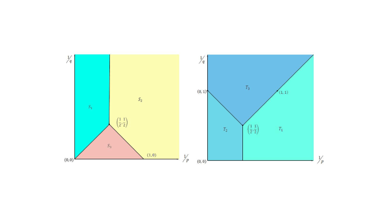
Figure 3: The left-hand side figure is for $\alpha_{1}\geqslant\alpha_{2}$; while the right-hand side figure is for $\alpha_{1}<\alpha_{2}$.

As $1\leq p,q\leq\infty$, some sufficient conditions for the inclusions between modulation and Besov spaces were obtained by Gröbner [11], then Toft [16] improved Gröbner’s sufficient conditions, which were proven to be necessary by Sugimoto and Tomita [15]. Their results were generalized to the cases $0<p,q\leq\infty$ in [19, 20]. Gröbner [11] also considered the inclusions between $\alpha_{1}$-modulation and $\alpha_{2}$-modulation spaces for $1\leq p,q\leq\infty$ and his results are optimal in the cases $(1/p,1/q)$ is located in the vertices of the square $[0,1]^{2}$. We will improve Gröbner’s results in the cases $1\leq p,q\leq\infty$ and our results also cover the cases $0<p<1$ or $0<q<1$.

4.1 Embedding between $\alpha$-modulation spaces

Theorem 4.1.

Let $(\alpha_{1},\alpha_{2})\in[0,1)\times[0,1)$. Then

$$M_{p,q}^{s_{1},\alpha_{1}}\subset M_{p,q}^{s_{2},\alpha_{2}}$$ (4.1)

holds if and only if $s_{1}\geqslant s_{2}+\mbox{R}(p,q;\alpha_{1},\alpha_{2})$.

Remark. In the first versions of the paper, we obtain the sufficiency of Theorem 4.1, soon after Toft and Wahlberg [17] independently considered the embeddings between $\alpha$-modulation and Besov spaces in the cases $1\leq p,q\leq\infty$ and they first showed the necessity of Theorem 4.1 in the regions $(1/p,1/q)\in(S_{2}\cup S_{3})\cap[0,1]^{2}$ (see Fig. 3). After their work we can finally show the necessity of Theorem 4.1 in all cases.

Proof.

(Sufficiency) For every $k\in\mathbb{Z}^{n}$, we introduce

$$\Lambda(k)=\{l\in\mathbb{Z}^{n}:\square_{l}^{\alpha_{2}}\square_{k}^{\alpha_{1}}f\neq 0\}.$$ (4.2)

If $\square_{l}^{\alpha_{2}}\square_{k}^{\alpha_{1}}f\neq 0$, then $k$ and $l$ satisfy

$$\begin{split}\langle l\rangle^{\frac{\alpha_{2}}{1-\alpha_{2}}}(l_{j}-C)&<\langle k\rangle^{\frac{\alpha_{1}}{1-\alpha_{1}}}(k_{j}+C),\\ \langle l\rangle^{\frac{\alpha_{2}}{1-\alpha_{2}}}(l_{j}+C)&>\langle k\rangle^{\frac{\alpha_{1}}{1-\alpha_{1}}}(k_{j}-C)\end{split}$$ (4.3)

for all $j=1,2,\cdots,n$. If $|k|\lesssim 1$, it is easy to see that $|l|\lesssim 1$. If $|k|\gg 1$, analogous to (3.12), we have

$$\langle l\rangle\sim\langle k\rangle^{\frac{1-\alpha_{2}}{1-\alpha_{1}}}.$$ (4.4)

Assume that $p\geqslant 1$, $q=1$ and $s_{2}=0$, we have

$$\|f\|_{M_{p,1}^{0,\alpha_{2}}}\leqslant\sum_{k\in\mathbb{Z}^{n}}\sum_{l\in\Lambda(k)}\|\square_{k}^{\alpha_{1}}\square_{l}^{\alpha_{2}}f\|_{p}\lesssim\sum_{k}\#\Lambda(k)\|\square_{k}^{\alpha_{1}}f\|_{p}.$$ (4.5)

We need an estimate of $\#\Lambda(k)$. Similar to (3.13), we have

$$\#\Lambda(k)\sim 1\vee\langle k\rangle^{\frac{n(\alpha_{1}-\alpha_{2})}{1-\alpha_{1}}}.$$ (4.6)

If $p=2$, inserting (4.6) into (4.5) and noticing (4.4), in view of Jensen’s inequality we get

$$M_{2,1}^{s_{2}+0\vee\frac{n(\alpha_{1}-\alpha_{2})}{2(1-\alpha_{1})},\alpha_{1}}\hookrightarrow M_{2,1}^{s_{2},\alpha_{2}}.$$ (4.7)

If $p=\infty$ or 1, from (4.5), (4.6), (4.4), one can directly obtain that

$$M_{\infty,1}^{s_{2}+0\vee\frac{n(\alpha_{1}-\alpha_{2})}{1-\alpha_{1}},\alpha_{1}} \hookrightarrow M_{\infty,1}^{s_{2},\alpha_{2}},$$ (4.8)

$$M_{1,1}^{s_{2}+0\vee\frac{n(\alpha_{1}-\alpha_{2})}{1-\alpha_{1}},\alpha_{1}} \hookrightarrow M_{1,1}^{s_{2},\alpha_{2}}.$$ (4.9)

Case 1: $\bm{\big{(}\frac{1}{p},\frac{1}{q}\big{)}\in\mbox{I}}.$ For any $\theta\in[0,1]$, $\big{(}\frac{\theta}{2},1\big{)}$ is at the line connecting $\big{(}\frac{1}{2},1\big{)}$ and $(0,1)$. By complex interpolation between (4.7) and (4.8), one has that

$$\begin{split}M_{\frac{2}{\theta},1}^{0\vee\big{(}1-\frac{\theta}{2}\big{)}\frac{n(\alpha_{1}-\alpha_{2})}{1-\alpha_{1}},\alpha_{1}}\hookrightarrow M_{\frac{2}{\theta},1}^{0,\alpha_{2}}.\end{split}$$ (4.10)

Since $\big{(}\frac{\theta}{2},1-\frac{\theta}{2}\big{)}$ is at the line segment by connecting $\big{(}\frac{1}{2},\frac{1}{2}\big{)}$ and $(0,1)$, A complex interpolation combined with Proposition 2.7 and (4.8) yields

$$\begin{split}M_{\frac{2}{\theta},\frac{2}{2-\theta}}^{0\vee(1-\theta)\frac{n(\alpha_{1}-\alpha_{2})}{1-\alpha_{1}}}\hookrightarrow M_{\frac{2}{\theta},\frac{2}{2-\theta}}^{0,\alpha_{2}}.\end{split}$$ (4.11)

For any $\big{(}\frac{1}{p},\frac{1}{q}\big{)}\in\mbox{I}$, we may suppose that there exists some $(\theta,\eta)\in[0,1]\times[0,1]$, such that

$$\frac{1}{p}=\frac{1}{p_{1}}=\frac{\theta}{2},\qquad\frac{1}{q}=1-\frac{\theta\eta}{2}.$$

Therefore, a complex interpolation between (4.10) and (4.11) implies that

$$\begin{split}M_{p,q}^{s_{2}+\big{(}\frac{1}{q}-\frac{1}{p}\big{)}[0\vee n(\alpha_{1}-\alpha_{2})],\alpha_{1}}\hookrightarrow M_{p,q}^{s_{2},\alpha_{2}}.\end{split}$$ (4.12)

Case 2: $\bm{\big{(}\frac{1}{p},\frac{1}{q}\big{)}\in\mbox{II}}.$ For any $\theta\in[0,1]$, $\big{(}1-\frac{\theta}{2},1-\frac{\theta}{2}\big{)}$ is at the line segment connecting $\big{(}\frac{1}{2},\frac{1}{2}\big{)}$ and $(1,1)$. From Proposition 2.7 and (4.9), we see that

$$M_{\frac{2}{2-\theta},\frac{2}{2-\theta}}^{s_{2}+(1-\theta)[0\vee n(\alpha_{1}-\alpha_{2})],\alpha_{1}}\hookrightarrow M_{\frac{2}{2-\theta},\frac{2}{2-\theta}}^{s_{2},\alpha_{2}}.$$ (4.13)

Noticing that $\big{(}1-\frac{\theta}{2},1\big{)}$ is a point at the line segment connecting $\big{(}\frac{1}{2},1\big{)}$ and $(0,1)$, from (4.7) and (4.9), we see that

$$M_{\frac{2}{2-\theta},1}^{s_{2}+\big{(}1-\frac{\theta}{2}\big{)}[0\vee n(\alpha_{1}-\alpha_{2})],\alpha_{1}}\hookrightarrow M^{s_{2},\alpha_{2}}_{\frac{2}{2-\theta},1}.$$ (4.14)

Noticing that for any $\big{(}\frac{1}{p},\frac{1}{q}\big{)}\in\mbox{II}$, there exists some $(\theta,\eta)\in[0,1]\times[0,1]$ satisfying

$$\frac{1}{p}=1-\frac{\theta}{2},\qquad\frac{1}{q}=1-\frac{\theta\eta}{2},$$

on the basis of (4.13) and (4.14), we conclude that

$$M_{p,q}^{s_{2}+\big{(}\frac{1}{p}+\frac{1}{q}-1\big{)}[0\vee n(\alpha_{1}-\alpha_{2})],\alpha_{1}}\hookrightarrow M_{p,q}^{s_{2},\alpha_{2}}.$$ (4.15)

When $\alpha_{1}\leqslant\alpha_{2}$, (4.15) coincides with (4.12).

Case 3: $\bm{\big{(}\frac{1}{p},\frac{1}{q}\big{)}\in\mbox{I}^{\ast}\cup\mbox{II}^{\ast}}.$ When $\big{(}\frac{1}{p},\frac{1}{q}\big{)}\in\mbox{I}^{\ast}$, $\big{(}\frac{1}{p^{*}},\frac{1}{q^{*}}\big{)}$ is in I. From (4.12), we know

$$M_{p^{\ast},q^{\ast}}^{-s_{2},\alpha_{2}}\hookrightarrow M_{p^{\ast},q^{\ast}}^{-s_{2}-\big{(}\frac{1}{p}-\frac{1}{q}\big{)}[0\vee n(\alpha_{2}-\alpha_{1})],\alpha_{1}}.$$

The duality of $\alpha$-modulation space implies that

$$M_{p,q}^{s_{2}+\big{(}\frac{1}{p}-\frac{1}{q}\big{)}[0\vee n(\alpha_{2}-\alpha_{1})],\alpha_{1}}\hookrightarrow M_{p,q}^{s_{2},\alpha_{2}}.$$ (4.16)

When $\big{(}\frac{1}{p},\frac{1}{q}\big{)}\in\mbox{II}^{\ast}$, by (4.15) and duality one has that

$$M_{p,q}^{s_{2}+\big{(}1-\frac{1}{p}-\frac{1}{q}\big{)}[0\vee n(\alpha_{2}-\alpha_{1})],\alpha_{1}}\hookrightarrow M_{p,q}^{s_{2},\alpha_{2}}.$$ (4.17)

When $\alpha_{1}>\alpha_{2}$, (4.17) coincides with (4.16).

Case 4: $\bm{\big{(}\frac{1}{p},\frac{1}{q}\big{)}\in\mbox{III}\cup\mbox{III}^{*}}.$ We may assume that for any $\big{(}\frac{1}{p},\frac{1}{q}\big{)}\in\mbox{III}\;(\mbox{III}^{*})$, there exists a $\eta\in(0,1)$ satisfying

$$\frac{1}{q}=\eta\left(1-\frac{1}{p}\right)+\frac{1-\eta}{p}.$$

Notice that $\big{(}\frac{1}{p},\frac{1}{p}\big{)}$ and $\big{(}\frac{1}{p},1-\frac{1}{p}\big{)}$ are at the boundaries of II and $\mbox{I}^{*}$ ($\mbox{II}^{*}$ and I), respectively. If $\big{(}\frac{1}{p},\frac{1}{q}\big{)}\in\mbox{III}$, a complex interpolation between (4.15) and (4.16) yields

$$M_{p,q}^{s_{2}+\left[n(\alpha_{1}-\alpha_{2})\big{(}\frac{1}{p}+\frac{1}{q}-1\big{)}\vee n(\alpha_{2}-\alpha_{1})\big{(}\frac{1}{p}-\frac{1}{q}\big{)}\right],\alpha_{1}}\hookrightarrow M_{p,q}^{s_{2},\alpha_{2}};$$ (4.18)

If $\big{(}\frac{1}{p},\frac{1}{q}\big{)}\in\mbox{III}^{*}$, a complex interpolation between (4.12) and (4.17) yields

$$M_{p,q}^{s_{2}+\left[n(\alpha_{1}-\alpha_{2})\big{(}\frac{1}{q}-\frac{1}{p}\big{)}\vee n(\alpha_{2}-\alpha_{1})\big{(}1-\frac{1}{p}-\frac{1}{q}\big{)}\right],\alpha_{1}}\hookrightarrow M_{p,q}^{s_{2},\alpha_{2}}.$$ (4.19)

When $\alpha_{1}>\alpha_{2}$, (4.18) and (4.19) coincide with (4.15) and (4.12), respectively. When $\alpha_{1}\leqslant\alpha_{2}$, (4.18) and (4.19) coincide with (4.16) and (4.17), respectively.

Case 5: $\bm{\big{(}\frac{1}{p},\frac{1}{q}\big{)}\in\widehat{\mbox{I}}.}$ Imitating the proof as in the counterpart of Theorem 3.1, we can easily get

$$M_{\infty,q}^{s_{2}+0\vee\frac{n(\alpha_{1}-\alpha_{2})}{1-\alpha_{1}}\frac{1}{q},\alpha_{1}}\subset M_{\infty,q}^{s_{2},\alpha_{2}},\quad M_{2,q}^{s_{2}+0\vee\frac{n(\alpha_{1}-\alpha_{2})}{1-\alpha_{1}}\big{(}\frac{1}{q}-\frac{1}{2}\big{)},\alpha_{1}}\subset M_{2,q}^{s_{2},\alpha_{2}}.$$

A complex interpolation yields

$$M_{p,q}^{s_{2}+0\vee\frac{n(\alpha_{1}-\alpha_{2})}{1-\alpha_{1}}\big{(}\frac{1}{q}-\frac{1}{p}\big{)},\alpha_{1}}\subset M_{p,q}^{s_{2},\alpha_{2}}.$$ (4.20)

(4.20) coincides with (4.12).

Case 6: $\bm{\big{(}\frac{1}{p},\frac{1}{q}\big{)}\in\widehat{\mbox{III}}.}$ From (1.1b), as well as (4.4), we see that

$$\mbox{diam}\;\mbox{supp}\mathscr{F}[\mathscr{F}^{-1}\eta_{l}^{\alpha_{2}}(x-\cdot)\square_{k}^{\alpha_{1}}f(\cdot)]\lesssim\langle k\rangle^{\frac{\alpha_{1}\vee\alpha_{2}}{1-\alpha_{1}}},$$

In view of Proposition 2.1,

$$\|\square_{l}^{\alpha_{2}}\square_{k}^{\alpha_{1}}f\|_{p}\lesssim\langle k\rangle^{\big{(}\frac{1}{p}-1\big{)}\frac{0\vee n(\alpha_{1}-\alpha_{2})}{1-\alpha_{1}}}\|\square_{k}^{\alpha_{1}}f\|_{p}.$$ (4.21)

Inserting (4.21), (4.4), (4.6), from the embedding $\ell^{p}\subset\ell^{1}$ and with the aid of Jensen’s inequality, we have

$$\begin{split}\|f\|_{M_{p,q}^{s_{2},\alpha_{2}}}&\lesssim\left[\sum_{l\in\mathbb{Z}^{n}}\langle l\rangle^{\frac{s_{2}q}{1-\alpha_{2}}}\left(\sum_{k\in\Lambda(l)}\langle k\rangle^{(1-p)\frac{0\vee n(\alpha_{1}-\alpha_{2})}{1-\alpha_{1}}}\|\square_{k}^{\alpha_{1}}f\|_{p}^{p}\right)^{\frac{q}{p}}\right]^{\frac{1}{q}}\\ &\lesssim\left(\sum_{l}\langle l\rangle^{\frac{s_{2}q}{1-\alpha_{2}}+\frac{0\vee n(\alpha_{2}-\alpha_{1})}{1-\alpha_{2}}\big{(}\frac{q}{p}-1\big{)}}\sum_{k\in\Lambda(l)}\langle k\rangle^{nq\big{(}\frac{1}{p}-1\big{)}\frac{0\vee(\alpha_{1}-\alpha_{2})}{1-\alpha_{1}}}\|\square_{k}^{\alpha_{1}}f\|_{p}^{q}\right)^{\frac{1}{q}}\\ &\lesssim\left(\sum_{k}\langle k\rangle^{\frac{s_{2}q}{1-\alpha_{1}}+\frac{0\vee n(\alpha_{2}-\alpha_{1})}{1-\alpha_{1}}\big{(}\frac{q}{p}-1\big{)}+nq\frac{0\vee(\alpha_{1}-\alpha_{2})}{1-\alpha_{1}}\big{(}\frac{1}{p}+\frac{1}{q}-1\big{)}}\|\square_{k}^{\alpha_{1}}f\|_{p}^{q}\right)^{\frac{1}{q}}.\end{split}$$ (4.22)

When $\alpha_{1}\leqslant\alpha_{2}$, (4.22) gives

$$M_{p,q}^{s_{2}+n(\alpha_{2}-\alpha_{1})\big{(}\frac{1}{p}-\frac{1}{q}\big{)},\alpha_{1}}\subset M_{p,q}^{s_{2},\alpha_{2}};$$ (4.23)

whereas when $\alpha_{1}>\alpha_{2}$, (4.22) gives

$$M_{p,q}^{s_{2}+n(\alpha_{1}-\alpha_{2})\big{(}\frac{1}{p}+\frac{1}{q}-1\big{)},\alpha_{1}}\subset M_{p,q}^{s_{2},\alpha_{2}}.$$ (4.24)

(4.23) and (4.24) coincide with (4.16) and (4.15), respectively.

Case 7: $\bm{\big{(}\frac{1}{p},\frac{1}{q}\big{)}\in\widehat{\mbox{II}}.}$ This is a consequence of the results in Cases 5 and 6 by complex interpolation. MM $\square$

4.2 Embedding between Besov space and $\alpha$-modulation space

In this section, we study the embedding between 1-modulation space and $\alpha$-modulation spaces. In an analogous way to the previous subsection, we start with the embedding for the same indices $p,q$.

Theorem 4.2.

Let $\alpha\in[0,1)$. Then $B_{p,q}^{s_{1}}\subset M_{p,q}^{s_{2},\alpha}$ holds if and only if $s_{1}\geqslant s_{2}+\mbox{R}(p,q;1,\alpha)$. Conversely, $M_{p,q}^{s_{1},\alpha}\subset B_{p,q}^{s_{2}}$ holds if and only if $s_{1}\geqslant s_{2}+\mbox{R}(p,q;\alpha,1)$.

Proof.

(sufficiency) For every $j\in\mathbb{Z}_{+}$, we introduce

$$\Lambda(j)=\{k\in\mathbb{Z}^{n}:\square_{k}^{\alpha}\triangle_{j}f\neq 0,\forall f\in\mathscr{S}^{\prime}(\mathbb{R}^{n})\};$$ (4.25)

and for every $k\in\mathbb{Z}^{n}$, we introduce

$$\Lambda(k)=\{j\in\mathbb{Z}_{+}:\square_{k}^{\alpha}\triangle_{j}f\neq 0,\forall f\in\mathscr{S}^{\prime}(\mathbb{R}^{n})\}.$$ (4.26)

To a $j\in\mathbb{Z}_{+}$, for any $k\in\Lambda(j)$, it is easy to see that the quantitative relationship between $k$ and $j$ is

$$\langle k\rangle^{\frac{1}{1-\alpha}}\sim 2^{j}.$$ (4.27)

When $p\geqslant 1,q=1$ and $s_{2}=0$, we have

$$\|f\|_{M_{p,1}^{0,\alpha}}\leqslant\sum_{k\in\mathbb{Z}^{n}}\sum_{j\in\Lambda(k)}\|\square_{k}^{\alpha}\triangle_{j}f\|_{p}=\sum_{j\in\mathbb{Z}_{+}}\sum_{k\in\Lambda(j)}\|\triangle_{j}\square_{k}^{\alpha}f\|_{p}.$$ (4.28)

For any $k\in\mathbb{Z}^{n}$ and any $j\in\mathbb{Z}_{+}$, it is easy to see

$$\#\Lambda(k)\sim 1,\quad\#\Lambda(j)\sim 2^{jn(1-\alpha)}.$$ (4.29)

Thus when $p=2$, combining (4.28), (4.29), also with the aid of Jensen’s inequality, we get

$$B_{2,1}^{s+\frac{n(1-\alpha)}{2}}\hookrightarrow M_{2,1}^{s,\alpha}.$$ (4.30)

If $p=1$ or $\infty$, combining (4.29), (4.28), we get

$$B_{1,1}^{s+n(1-\alpha)} \hookrightarrow M_{1,1}^{s,\alpha},$$ (4.31)

$$B_{\infty,1}^{s+n(1-\alpha)} \hookrightarrow M_{\infty,1}^{s,\alpha}.$$ (4.32)

${\bf Case1.}\ \bm{\big{(}\frac{1}{p},\frac{1}{q}\big{)}\in\mbox{I}}.$ For any $\theta\in[0,1]$, a complex interpolation between (4.30) and (4.32) yields

$$B_{\frac{2}{\theta},1}^{s+\big{(}1-\frac{\theta}{2}\big{)}n(1-\alpha)}\hookrightarrow M_{\frac{2}{\theta},1}^{s,\alpha};$$ (4.33)

while combined with Proposition 2.7 and (4.32), yields

$$B_{\frac{2}{\theta},\frac{2}{2-\theta}}^{s+(1-\theta)n(1-\alpha)}\hookrightarrow M_{\frac{2}{\theta},\frac{2}{2-\theta}}^{s,\alpha}.$$ (4.34)

In analogy to (4.12), we get from (4.33), (4.34) that

$$B_{p,q}^{s+n\big{(}\frac{1}{q}-\frac{1}{p}\big{)}(1-\alpha)}\hookrightarrow M_{p,q}^{s,\alpha}.$$ (4.35)

Conversely, when we encounter the embedding of $\alpha$-modulation spaces into Besov spaces, for $2\leqslant p\leqslant\infty$, considering (4.29), we have

$$\begin{split}\|f\|_{B_{p,1}^{0}}&\leqslant\sum_{j\in\mathbb{Z}^{+}}\sum_{k\in\Lambda(j)}\|\square_{k}^{\alpha}\triangle_{j}f\|_{p}\lesssim\sum_{k\in\mathbb{Z}^{n}}\|\square_{k}^{\alpha}f\|_{p}=\|f\|_{M_{p,1}^{0,\alpha}},\end{split}$$ (4.36)

which gives

$$M_{p,q}^{s,\alpha}\hookrightarrow B_{p,q}^{s}.$$ (4.37)

${\bf Case2.}\ \bm{\big{(}\frac{1}{p},\frac{1}{q}\big{)}\in\mbox{II}}.$ For any $\theta\in[0,1]$, a complex interpolation between (4.30) and (4.31) yields

$$B_{\frac{2}{2-\theta},1}^{s+\big{(}1-\frac{\theta}{2}\big{)}n(1-\alpha)}\hookrightarrow M_{\frac{2}{2-\theta},1}^{s,\alpha}.$$ (4.38)

From Proposition 2.7 and (4.31) it follows that

$$B_{\frac{2}{2-\theta},\frac{2}{2-\theta}}^{s+(1-\theta)n(1-\alpha)}\hookrightarrow M_{\frac{2}{2-\theta},\frac{2}{2-\theta}}^{s,\alpha}.$$ (4.39)

Analogous to (4.15), one can conclude from (4.38) and (4.39) that

$$B_{p,q}^{s+n\big{(}\frac{1}{q}+\frac{1}{p}-1\big{)}(1-\alpha)}\hookrightarrow M_{p,q}^{s,\alpha}.$$ (4.40)

Considering the embedding of $\alpha$-modulation spaces into Besov spaces, (4.37) still holds if $(1/p,1/q)\in II.$

${\bf Case3.}\ \bm{\big{(}\frac{1}{p},\frac{1}{q}\big{)}\in\mbox{I}^{\ast}\cup\mbox{II}^{\ast}}.$ Since $\big{(}\frac{1}{p^{*}},\frac{1}{q^{*}}\big{)}\in\mbox{I}\cup\mbox{II}$, from (4.37), we see that $M_{p^{\ast},q^{\ast}}^{-s,\alpha}\hookrightarrow B_{p^{\ast},q^{\ast}}^{-s}$. Thus, the duality between $B_{p,q}^{s}$ and $B_{p^{\ast},q^{\ast}}^{-s}$, as well as between $M_{p,q}^{s,\alpha}$ and $M_{p^{\ast},q^{\ast}}^{-s,\alpha}$, implies that

$$B_{p,q}^{s}\hookrightarrow M_{p,q}^{s,\alpha}.$$ (4.41)

Conversely, if one considers the embedding of $\alpha$-modulation space into Besov space, it follows from Theorem 2.1 and (4.35) that

$$M_{p,q}^{s+n(\alpha-1)\big{(}\frac{1}{q}-\frac{1}{p}\big{)},\alpha}\subset B_{p,q}^{s},\ \ \left(\frac{1}{p},\frac{1}{q}\right)\in\mbox{I}^{*};$$ (4.42)

and from (4.40) it follows that

$$M_{p,q}^{s+n(\alpha-1)\big{(}\frac{1}{p}+\frac{1}{q}-1\big{)},\alpha}\subset B_{p,q}^{s},\ \ \left(\frac{1}{p},\frac{1}{q}\right)\in\mbox{II}^{*}.$$ (4.43)

${\bf Case4.}\ \bm{\big{(}\frac{1}{p},\frac{1}{q}\big{)}\in\mbox{III}\cup\mbox{III}^{*}}.$ If $\big{(}\frac{1}{p},\frac{1}{q}\big{)}\in\mbox{III}^{*}$, (4.35) and (4.41) contain that

$$\begin{split}B_{p,\frac{p}{p-1}}^{s+n\big{(}1-\frac{2}{p}\big{)}(1-\alpha)}\hookrightarrow M_{p,\frac{p}{p-1}}^{s,\alpha},\quad B_{p,p}^{s}\hookrightarrow M_{p,p}^{s,\alpha}.\end{split}$$

By interpolation we have

$$B_{p,q}^{s+n\big{(}\frac{1}{q}-\frac{1}{p}\big{)}(1-\alpha)}\hookrightarrow M_{p,q}^{s,\alpha},$$ (4.44)

which coincides with (4.35). If $\big{(}\frac{1}{p},\frac{1}{q}\big{)}\in\mbox{III}$, (4.40) and (4.41) imply that

$$\begin{split}B_{p,\frac{p}{p-1}}^{s}\subset M_{p,\frac{p}{p-1}}^{s,\alpha},\quad B_{p,p}^{s+n\big{(}\frac{2}{p}-1\big{)}(1-\alpha)}\subset M_{p,q}^{s,\alpha}.\end{split}$$

By interpolation,

$$B_{p,q}^{s+n\big{(}\frac{1}{q}+\frac{1}{p}-1\big{)}(1-\alpha)}\hookrightarrow M_{p,q}^{s,\alpha},$$ (4.45)

which coincides with (4.40).

Conversely, considering the embedding of $\alpha$-modulation space into Besov space, in view of Theorem 2.1 and (4.44) we have

$$M_{p,q}^{s+n(\alpha-1)\big{(}\frac{1}{q}-\frac{1}{p}\big{)},\alpha}\subset B_{p,q}^{s},\ \ \left(\frac{1}{p},\frac{1}{q}\right)\in\mbox{III};$$ (4.46)

while for $\big{(}\frac{1}{p},\frac{1}{q}\big{)}\in\mbox{III}^{*}$, from (4.45), we have

$$M_{p,q}^{s+n(\alpha-1)\big{(}\frac{1}{p}+\frac{1}{q}-1\big{)},\alpha}\subset B_{p,q}^{s}.$$ (4.47)

(4.46) and (4.47) coincide with (4.42) and (4.43), respectively.

${\bf Case5:}\bm{\big{(}\frac{1}{p},\frac{1}{q}\big{)}\in\widehat{\mbox{I}}.}$ For the embedding of Besov space into $\alpha$-modulation space, imitating the argument in Theorem 4.1, we get

$$M_{\infty,q}^{s+n(1-\alpha)\frac{1}{q},1}\subset M_{p,q}^{s,\alpha},\quad M_{2,q}^{s+n(1-\alpha)\big{(}\frac{1}{q}-\frac{1}{2}\big{)},1}\subset M_{p,q}^{s,\alpha}.$$

From them, we interpolate out

$$M_{p,q}^{s+n(1-\alpha)\big{(}\frac{1}{q}-\frac{1}{p}\big{)},1}\subset M_{p,q}^{s,\alpha},$$ (4.48)

which coincides with (4.35). Conversely for the embedding of $\alpha$-modulation space into Besov space, we have

$$M_{p,q}^{s,\alpha}\subset B_{p,q}^{s},$$ (4.49)

which coincides with (4.37).

Case 6.   $\bm{\big{(}\frac{1}{p},\frac{1}{q}\big{)}\in\widehat{\mbox{III}}.}$ If $\Box^{\alpha}_{k}\triangle_{j}\neq 0$, then

$$\mbox{diam}\;\mbox{supp}\mathscr{F}[\mathscr{F}^{-1}\eta_{k}^{\alpha}(x-\cdot)\triangle_{j}f(\cdot)]\lesssim\langle k\rangle^{\frac{1}{1-\alpha}}\sim 2^{j},$$ (4.50)

So, in view of Proposition 2.1 we have

$$\|\square_{k}^{\alpha}\triangle_{j}f\|_{p}\lesssim\langle k\rangle^{\frac{n}{1-\alpha}\big{(}\frac{1}{p}-1\big{)}}\langle k\rangle^{-\frac{n\alpha}{1-\alpha}\big{(}\frac{1}{p}-1\big{)}}\|\triangle_{j}f\|_{p}\sim 2^{jn(1-\alpha)\big{(}\frac{1}{p}-1\big{)}}\|\triangle_{j}f\|_{p}.$$ (4.51)

From (4.51), (4.29), $\ell^{p}\subset\ell^{1}$ and Jensen’s inequality it follows that

$$\begin{split}\|f\|_{M_{p,q}^{s,\alpha}}&\lesssim\left[\sum_{k\in\mathbb{Z}^{n}}\langle k\rangle^{\frac{sq}{1-\alpha}}\left(\sum_{j\in\Lambda(k)}\|\square_{k}^{\alpha}\triangle_{j}f\|_{p}^{p}\right)^{\frac{q}{p}}\right]^{\frac{1}{q}}\\ &\lesssim\left(\sum_{k}\langle k\rangle^{\left[\frac{s}{1-\alpha}+n\big{(}\frac{1}{p}-1\big{)}\right]q}\sum_{j\in\Lambda(k)}\|\triangle_{j}f\|_{p}^{q}\right)^{\frac{1}{q}}\\ &\lesssim\left(\sum_{j}2^{j\left[s+n(1-\alpha)\big{(}\frac{1}{p}-1\big{)}\right]q}\sum_{k\in\Lambda(j)}\|\triangle_{j}f\|_{p}^{q}\right)^{\frac{1}{q}}\lesssim\|f\|_{B_{p,q}^{s+n(1-\alpha)\big{(}\frac{1}{p}+\frac{1}{q}-1\big{)}}},\end{split}$$ (4.52)

which implies that

$$B_{p,q}^{s+n(1-\alpha)\big{(}\frac{1}{p}+\frac{1}{q}-1\big{)},\alpha}\subset M_{p,q}^{s,\alpha}.$$ (4.53)

It coincides with (4.40).

Conversely, when we study the embedding of $\alpha$-modulation space into Besov space, in analogy to (4.50), we see

$$\mbox{diam}\;\mbox{supp}\mathscr{F}[\mathscr{F}^{-1}\varphi_{j}(x-\cdot)\square_{k}^{\alpha}f(\cdot)]\lesssim 2^{j}$$

In contrast to (4.51), we conclude

$$\|\triangle_{j}\square_{k}^{\alpha}f\|_{p}\lesssim 2^{jn\big{(}\frac{1}{p}-1\big{)}}2^{-jn\big{(}\frac{1}{p}-1\big{)}}\|\square_{k}^{\alpha}f\|_{p}=\|\square_{k}^{\alpha}f\|_{p}.$$ (4.54)

Inserting (4.54), the substitution for (4.52) is

$$\begin{split}\|f\|_{B_{p,q}^{s}}&\lesssim\left[\sum_{j\in\mathbb{Z}^{+}}2^{jsq}\left(\sum_{j\in\Lambda(j)}\|\triangle_{j}\square_{k}^{\alpha}f\|_{p}^{p}\right)^{\frac{q}{p}}\right]^{\frac{1}{q}}\\ &\lesssim\left(\sum_{j}2^{jsq}\#\Lambda(j)^{\frac{q}{p}-1}\sum_{k\in\Lambda(j)}\|\triangle_{j}\square_{k}^{\alpha}f\|_{p}^{q}\right)^{\frac{1}{q}}\\ &\lesssim\left(\sum_{k}\langle k\rangle^{\left[s+n(1-\alpha)\big{(}\frac{1}{p}-\frac{1}{q}\big{)}\right]q}\|\square_{k}^{\alpha}f\|_{p}^{q}\right)^{\frac{1}{q}}\lesssim\|f\|_{M_{p,q}^{s+n(1-\alpha)\big{(}\frac{1}{p}-\frac{1}{q}\big{)}}},\end{split}$$

which implies that

$$M_{p,q}^{s+n(\alpha-1)\big{(}\frac{1}{q}-\frac{1}{p}\big{)},\alpha}\subset M_{p,q}^{s,1}.$$ (4.55)

It coincides with (4.42).

${\bf Case7:}\bm{\big{(}\frac{1}{p},\frac{1}{q}\big{)}\in\widehat{\mbox{II}}.}$ It is interpolated out from Case 5 and Case 6. MM $\square$

5 Multiplication algebra

It is well known that $B_{p,q}^{s}$ is a multiplication algebra if $s>n/p$, cf. [18]. But for $\alpha$-modulation space, this issue is much more complicated. The regularity indices for which $M_{p,q}^{s,\alpha}$ constitutes a multiplication algebra, are quite different from those of Besov and modulation spaces.

We introduce a parameter, denoted by $s_{0}=s_{0}(p,q;\alpha)$, to describe the regularity for which $M_{p,q}^{s,\alpha}$ with $s>s_{0}$ forms a multiplication algebra. Denote (see Figure 4)

$$\mbox{D}_{1}=\left\{\big{(}\tfrac{1}{p},\tfrac{1}{q}\big{)}\in\mathbb{R}_{+}^{2}:\tfrac{1}{q}\geqslant\tfrac{2}{p},\tfrac{1}{p}\leqslant\tfrac{1}{2}\right\},\quad D_{2}=\mathbb{R}_{+}^{2}\setminus D_{1}$$

and

$$s_{0}=\begin{cases}\frac{n\alpha}{p}+n(1-\alpha)\big{(}1-1\wedge\frac{1}{q}\big{)}+\frac{n\alpha(1-\alpha)}{2-\alpha}\big{(}\frac{1}{q}-\frac{2}{p}\big{)},&\quad\big{(}\frac{1}{p},\frac{1}{q}\big{)}\in\mbox{D}_{1};\\ \frac{n\alpha}{p}+n(1-\alpha)\big{(}1\vee\frac{1}{p}\vee\frac{1}{q}-\frac{1}{q}\big{)}+\frac{n\alpha(1-\alpha)}{2-\alpha}\big{(}1\vee\frac{1}{p}\vee\frac{1}{q}-1\big{)},&\quad\big{(}\frac{1}{p},\frac{1}{q}\big{)}\in\mbox{D}_{2}.\end{cases}$$

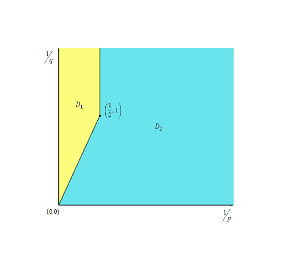
Figure 4: Distribution of $s_{0}$

Theorem 5.1.

If $s>s_{0}$, then $M_{p,q}^{s,\alpha}$ is a multiplication algebra, which is equivalent to say that for any $f,g\in M_{p,q}^{s,\alpha}$, we have

$$\|fg\|_{M_{p,q}^{s,\alpha}}\lesssim\|f\|_{M_{p,q}^{s,\alpha}}\|g\|_{M_{p,q}^{s,\alpha}}.$$ (5.1)

In Section 7 we will give some counterexamples to show that $s_{0}$ is sharp if $(1/p,1/q)\in\mbox{D}_{2}\cap\{p\geq 1\}$. When $\big{(}1/p,\;1/q\big{)}\in D_{1}$, it is not very clear for us to know the sharp low bound of the index $s$ for which $M_{p,q}^{s,\alpha}$ constitutes a multiplication algebra. As a straightforward consequence of Theorem 5.1, we have the following result for which $M^{s}_{p,q}$ is an algebra.

Corrolary 5.1.

Assume that

$$s>\begin{cases}n\big{(}1-1\wedge\frac{1}{q}\big{)},&\quad\big{(}\frac{1}{p},\frac{1}{q}\big{)}\in\mbox{D}_{1};\\ n\big{(}1\vee\frac{1}{p}\vee\frac{1}{q}-\frac{1}{q}\big{)},&\quad\big{(}\frac{1}{p},\frac{1}{q}\big{)}\in\mathbb{R}_{+}^{2}\backslash\mbox{D}_{1}.\end{cases}$$

Then $M_{p,q}^{s}$ is a multiplication algebra, i.e.,

$$\|fg\|_{M_{p,q}^{s}}\lesssim\|f\|_{M_{p,q}^{s}}\|g\|_{M_{p,q}^{s}}$$ (5.2)

holds for all $f,g\in M^{s}_{p,q}.$

A natural long standing question on modulation, $\alpha$-modulation and Besov spaces is: Can we reformulate $\alpha$-modulation spaces by interpolations between modulation and Besov spaces, say,

$$M^{s,\alpha}_{p,q}=(M^{s_{0},0}_{p,q},\ M^{s_{1},1}_{p,q})_{\alpha},\quad\mbox{if}\ \ s=(1-\alpha)s_{0}+\alpha s_{1}?$$ (5.3)

The answer is negative at least for some special cases. Indeed, we see $M^{s_{1},1}_{p,q}$ and $M^{s_{0},0}_{p,q}$ are algebra if $s_{1}>n/p$ and $s_{0}>0$. If (5.3) holds, then $M^{s,\alpha}_{p,q}$ is an algebra if $s>n\alpha/p$, however, this is not true if $1<p<2,\ 0<q<1$, see Section 7.

Corrolary 5.2.

Let $0<\alpha<1$. Then (5.3) does not hold if $1<p<2,\ 0<q<1$ and $s_{0}=0_{+},\ s_{1}=n/p$.

Proof of Theorem 5.1..

We start with some notations and basic conclusions. For every $(k^{(1)},k^{(2)})\in\mathbb{Z}^{2n}$, we introduce

$$\Lambda\big{(}k^{(1)},k^{(2)}\big{)}=\left\{k\in\mathbb{Z}^{n}:\square_{k}^{\alpha}(\square_{k^{(1)}}^{\alpha}f\square_{k^{(2)}}^{\alpha}g)\neq 0\right\};$$ (5.4)

and for every $k\in\mathbb{Z}^{n}$, we introduce

$$\Lambda(k)=\left\{\big{(}k^{(1)},k^{(2)}\big{)}\in\mathbb{Z}^{2n}:\square_{k}^{\alpha}(\square_{k^{(1)}}^{\alpha}f\square_{k^{(2)}}^{\alpha}g)\neq 0\right\}.$$

It is worth to mention that $\Lambda\big{(}k^{(1)},k^{(2)}\big{)}$ and $\Lambda(k)$ are independent of $f$ and $g$. From (1.1b) we see that for any $k\in\Lambda(k^{(1)},k^{(2)})$, or $(k^{(1)},k^{(2)})\in\Lambda(k)$, $k^{(1)},k^{(2)}$ and $k$ satisfy

$$\langle k\rangle^{\frac{\alpha}{1-\alpha}}(k_{j}-C)<\langle k^{(1)}\rangle^{\frac{\alpha}{1-\alpha}}(k^{(1)}_{j}+C)+\langle k^{(2)}\rangle^{\frac{\alpha}{1-\alpha}}(k^{(2)}_{j}+C),$$ (5.5a)

$$\langle k\rangle^{\frac{\alpha}{1-\alpha}}(k_{j}+C)>\langle k^{(1)}\rangle^{\frac{\alpha}{1-\alpha}}(k^{(1)}_{j}-C)+\langle k^{(2)}\rangle^{\frac{\alpha}{1-\alpha}}(k^{(2)}_{j}-C)$$ (5.5b)

for $j=1,2,\cdots,n$. Let $\langle k_{\max}\rangle$, $\langle k_{\rm min}\rangle$ and $\langle k_{\rm med}\rangle$ to be the maximal, minimal and medial ones in $\langle k\rangle,\langle k^{(1)}\rangle$ and $\langle k^{(2)}\rangle$, respectively. If (5.5) holds, then

$$\langle k_{\max}\rangle\sim\langle k_{\rm med}\rangle,\ \ \#\big{\{}k_{\max}:\ k_{\max},\ k_{\rm med},\ k_{\min}\ \mbox{satisfy}\ \eqref{rela}\big{\}}\lesssim 1.$$ (5.6)

We write

$$\begin{split}K_{j}\big{(}k^{(1)},k^{(2)}\big{)}&=\langle k^{(1)}\rangle^{\frac{\alpha}{1-\alpha}}k^{(1)}_{j}+\langle k^{(2)}\rangle^{\frac{\alpha}{1-\alpha}}k^{(2)}_{j};\\ K\big{(}k^{(1)},k^{(2)}\big{)}&=\max_{1\leqslant j\leqslant n}|K_{j}(k^{(1)},k^{(2)})|.\end{split}$$ (5.7)

In order to get more precise estimates, we divide $\mathbb{Z}^{2n}$ of all $(k^{(1)},k^{(2)})$ into

$$\begin{split}\Omega_{0}&=\left\{\big{(}k^{(1)},k^{(2)}\big{)}\in\mathbb{Z}^{2n}:\langle k^{(1)}\rangle\sim\langle k^{(2)}\rangle\right\},\\ \Omega_{1}&=\left\{\big{(}k^{(1)},k^{(2)}\big{)}\in\mathbb{Z}^{2n}:\langle k^{(1)}\rangle\gg\langle k^{(2)}\rangle\right\},\\ \Omega_{2}&=\left\{\big{(}k^{(1)},k^{(2)}\big{)}\in\mathbb{Z}^{2n}:\langle k^{(1)}\rangle\ll\langle k^{(2)}\rangle\right\},\end{split}$$ (5.8)

and separate $\Omega_{0}$ into

$$\begin{split}\Omega_{0,1}&=\left\{\big{(}k^{(1)},k^{(2)}\big{)}\in\Omega_{0}:K\big{(}k^{(1)},k^{(2)}\big{)}\lesssim\langle k^{(1)}\rangle^{\frac{\alpha}{1-\alpha}}\right\};\\ \Omega_{0,2}&=\left\{\big{(}k^{(1)},k^{(2)}\big{)}\in\Omega_{0}:K\big{(}k^{(1)},k^{(2)}\big{)}\gg\langle k^{(1)}\rangle^{\frac{\alpha}{1-\alpha}}\right\}.\end{split}$$ (5.9)

If $(k^{(1)},k^{(2)})\in\Omega_{0,1}$, from (5.5) it is easy to see that

$$\langle k\rangle\lesssim\langle k^{(1)}\rangle^{\alpha}.$$ (5.10)

Let $(k^{(1)},k^{(2)})\in\Omega_{0,2}$ be fixed. There exists some $y:=y(k^{(1)},k^{(2)})\in(\alpha,1]$ such that

$$K_{i}(k^{(1)},k^{(2)})=K(k^{(1)},k^{(2)})\sim\langle k^{(1)}\rangle^{\frac{y}{1-\alpha}},$$ (5.11)

for some $i$ with $1\leqslant i\leqslant n$. We can assume that $K_{i}(k^{(1)},k^{(2)})>0$. By (5.5) and (5.11) we have

$$\langle k\rangle^{\frac{\alpha}{1-\alpha}}(k_{i}-C)<K_{i}(k^{(1)},k^{(2)})+C(\langle k^{(1)}\rangle^{\frac{\alpha}{1-\alpha}}+\langle k^{(2)}\rangle^{\frac{\alpha}{1-\alpha}}) \lesssim\langle k^{(1)}\rangle^{\frac{y}{1-\alpha}},$$ (5.12a)

$$\langle k\rangle^{\frac{\alpha}{1-\alpha}}(k_{i}+C)>K_{i}(k^{(1)},k^{(2)})-C(\langle k^{(1)}\rangle^{\frac{\alpha}{1-\alpha}}+\langle k^{(2)}\rangle^{\frac{\alpha}{1-\alpha}}) \gtrsim\langle k^{(1)}\rangle^{\frac{y}{1-\alpha}}.$$ (5.12b)

For every $k\in\Lambda(k^{(1)},k^{(2)})\cap\mathbb{R}^{n}_{\widetilde{i}}$, we substitute $\widetilde{i}$ for $j$ in (5.5), thus (5.5a) and (5.5b) are rewritten as

$$\langle k\rangle^{\frac{\alpha}{1-\alpha}}(k_{\widetilde{i}}-C) <K_{\widetilde{i}}(k^{(1)},k^{(2)})+C(\langle k^{(1)}\rangle^{\frac{\alpha}{1-\alpha}}+\langle k^{(2)}\rangle^{\frac{\alpha}{1-\alpha}});$$ (5.13a)

$$\langle k\rangle^{\frac{\alpha}{1-\alpha}}(k_{\widetilde{i}}+C) >K_{\widetilde{i}}(k^{(1)},k^{(2)})-C(\langle k^{(1)}\rangle^{\frac{\alpha}{1-\alpha}}+\langle k^{(2)}\rangle^{\frac{\alpha}{1-\alpha}}).$$ (5.13b)

For such $k$, we claim that

$$\langle k\rangle\sim\langle k^{(1)}\rangle^{y}.$$ (5.14)

(5.14) is obvious when $|k^{(1)}|\lesssim 1$ and so, it suffices to consider (5.14) in the case $|k^{(1)}|\gg 1$. If either $|k_{i}|\sim\langle k\rangle$ or $|K_{\widetilde{i}}(k^{(1)},k^{(2)})|\sim K(k^{(1)},k^{(2)})$ exists, (5.14) follows from (5.12) or (5.13) directly. Otherwise, we see that $|k_{i}|\ll\langle k\rangle$ and $|K_{\widetilde{i}}(k^{(1)},k^{(2)})|\ll K(k^{(1)},k^{(2)})$. When $k_{\widetilde{i}}>0$, we let (5.13a)+(5.12a) and (5.13b)+(5.12b); whereas when $k_{\widetilde{i}}<0$, we let (5.13b)$\times(-1)+$(5.12a) and (5.12a)$\times(-1)+$(5.12b), then we get

$$\langle k\rangle^{\frac{1}{1-\alpha}}\gtrsim\langle k^{(1)}\rangle^{\frac{y}{1-\alpha}},\quad\langle k\rangle^{\frac{1}{1-\alpha}}\lesssim\langle k^{(1)}\rangle^{\frac{y}{1-\alpha}},$$

which imply (5.14). Let $\widetilde{k}=(k_{1},...,k_{j-1},\tilde{k}_{j},k_{j+1},...,k_{n})\in\Lambda(k^{(1)},k^{(2)})$. In view of (5.5a) and (5.5b) and $(k^{(1)},k^{(2)})\in\Omega_{0,2}$, we have

$$\left|\langle k\rangle^{\frac{\alpha}{1-\alpha}}k_{j}-\langle\widetilde{k}\rangle^{\frac{\alpha}{1-\alpha}}\widetilde{k}_{j}\right|\lesssim\langle k^{(1)}\rangle^{\frac{\alpha}{1-\alpha}}+\langle k\rangle^{\frac{\alpha}{1-\alpha}}+\langle\widetilde{k}\rangle^{\frac{\alpha}{1-\alpha}}.$$

Thus Taylor’s theorem, combined with (5.14), gives

$$\left|k_{j}-\widetilde{k}_{j}\right|\lesssim\langle k^{(1)}\rangle^{\frac{\alpha(1-y)}{1-\alpha}}.$$ (5.15)

For $\big{(}k^{(1)},k^{(2)}\big{)}\in\Omega_{1}\cup\Omega_{2}$, in view of (5.6) we have

$$\langle k\rangle\sim\langle k^{(1)}\rangle\vee\langle k^{(2)}\rangle$$ (5.16)

and

$$\#\Lambda\big{(}k^{(1)},k^{(2)}\big{)}\sim 1.$$ (5.17)

In what follows, we separate the proof into four steps. In Steps 1-3, we prove (5.1) for certain $p$ and $q$. In Step 4, applying the complex interpolation together with the conclusions obtained in the previous three steps, we can get (5.1).

Step 1. $\bm{1\leqslant p\leqslant\infty,q\leqslant 1.}$ Suppose $f,g\in M_{p,q}^{s,\alpha}$, from the triangle inequality and the embedding $\ell^{q}\subset\ell^{1}$, we have

$$\begin{split}\|fg\|_{M_{p,q}^{s,\alpha}}&=\left(\sum_{k\in\mathbb{Z}^{n}}\langle k\rangle^{\frac{sq}{1-\alpha}}\|\square_{k}^{\alpha}(fg)\|_{p}^{q}\right)^{\frac{1}{q}}\\ &\leqslant\left[\sum_{k}\langle k\rangle^{\frac{sq}{1-\alpha}}\left(\sum_{k^{(1)},k^{(2)}}\|\square_{k}^{\alpha}(\square_{k^{(1)}}^{\alpha}f\square_{k^{(2)}}^{\alpha}g)\|_{p}\right)^{q}\right]^{\frac{1}{q}}\\ &\leqslant\left(\sum_{k}\langle k\rangle^{\frac{sq}{1-\alpha}}\sum_{k^{(1)},k^{(2)}}\|\square_{k}^{\alpha}(\square_{k^{(1)}}^{\alpha}f\square_{k^{(2)}}^{\alpha}g)\|_{p}^{q}\right)^{\frac{1}{q}}\\ &=\left(\sum_{\ell=0}^{2}\sum_{(k^{(1)},k^{(2)})\in\Omega_{\ell}}\sum_{k\in\Lambda(k^{(1)},k^{(2)})}\langle k\rangle^{\frac{sq}{1-\alpha}}\|\square_{k}^{\alpha}(\square_{k^{(1)}}^{\alpha}f\square_{k^{(2)}}^{\alpha}g)\|_{p}^{q}\right)^{\frac{1}{q}}.\end{split}$$ (5.18)

Applying the multiplier estimate and Hölder’s inequality, we see that

$$\|\square_{k}^{\alpha}(\square_{k^{(1)}}^{\alpha}f\square_{k^{(2)}}^{\alpha}g)\|_{p}\lesssim\|\square_{k^{(1)}}^{\alpha}f\square_{k^{(2)}}^{\alpha}g\|_{p}\lesssim\|\square_{k^{(1)}}^{\alpha}f\|_{p}\|\square_{k^{(2)}}^{\alpha}g\|_{\infty}.$$ (5.19)

For $(k^{(1)},k^{(2)})\in\Omega_{0,1}$, when $p=1$ and $s\geqslant n\alpha+\frac{n\alpha(1-\alpha)}{2-\alpha}\big{(}\frac{1}{q}-1\big{)}$, we have

$$\begin{split}&\sum_{(k^{(1)},k^{(2)})\in\Omega_{0,1}}\sum_{k\in\Lambda(k^{(1)},k^{(2)})}\langle k\rangle^{\frac{sq}{1-\alpha}}\|\square_{k}^{\alpha}(\square_{k^{(1)}}^{\alpha}f\square_{k^{(2)}}^{\alpha}g)\|_{1}^{q}\\ &\qquad\lesssim\sum_{(k^{(1)},k^{(2)})}\langle k^{(1)}\rangle^{\frac{sq\alpha}{1-\alpha}+n\alpha}\|\square_{k^{(1)}}^{\alpha}f\|_{1}^{q}\langle k^{(2)}\rangle^{\frac{nq\alpha}{1-\alpha}}\|\square_{k^{(2)}}^{\alpha}g\|_{1}^{q}\leqslant\|f\|_{M_{1,q}^{s,\alpha}}^{q}\|g\|_{M_{1,q}^{s,\alpha}}^{q}.\end{split}$$ (5.20)

If $p=2$ and $s\geqslant\frac{n\alpha}{2}+\frac{n\alpha(1-\alpha)}{2-\alpha}\big{(}\frac{1}{q}-1\big{)}$, by Plancherel and Jensen’s inequality, we have

$$\begin{split}&\sum_{(k^{(1)},k^{(2)})\in\Omega_{0,1}}\sum_{k\in\Lambda(k^{(1)},k^{(2)})}\langle k\rangle^{\frac{sq}{1-\alpha}}\|\square_{k}^{\alpha}(\square_{k^{(1)}}^{\alpha}f\square_{k^{(2)}}g)\|_{2}^{q}\\ &\qquad\lesssim\sum_{(k^{(1)},k^{(2)})}\sup_{k\in\Lambda(k^{(1)},k^{(2)})}\langle k\rangle^{\frac{sq}{1-\alpha}}\sum_{k\in\Lambda(k^{(1)},k^{(2)})}\|\square_{k}^{\alpha}(\square_{k^{(1)}}^{\alpha}f\square_{(2)}^{\alpha}g)\|_{2}^{q}\\ &\qquad\lesssim\sum_{(k^{(1)},k^{(2)})}\langle k^{(1)}\rangle^{\frac{sq\alpha}{1-\alpha}}[\#\Lambda(k^{(1)},k^{(2)})]^{1-\frac{q}{2}}\|\square_{k^{(1)}}^{\alpha}f\square_{k^{(2)}}^{\alpha}g\|_{2}^{q}\\ &\qquad\lesssim\sum_{(k^{(1)},k^{(2)})}\langle k^{(1)}\rangle^{\frac{sq\alpha}{1-\alpha}+n\alpha\big{(}1-\frac{q}{2}\big{)}}\|\square_{k^{(1)}}^{\alpha}f\|_{2}^{q}\langle k^{(2)}\rangle^{\frac{nq\alpha}{2(1-\alpha)}}\|\square_{k^{(2)}}^{\alpha}g\|_{2}^{q}\leqslant\|f\|_{M_{2,q}^{s,\alpha}}^{q}\|g\|_{M_{2,q}^{s,\alpha}}^{q}.\end{split}$$ (5.21)

For $p=\infty$ and $s\geqslant\frac{n\alpha(1-\alpha)}{2-\alpha}\frac{1}{q}$, we have

$$\begin{split}&\sum_{(k^{(1)},k^{(2)})\in\Omega_{0,1}}\sum_{k\in\Lambda(k^{(1)},k^{(2)})}\langle k\rangle^{\frac{sq}{1-\alpha}}\|\square_{k}^{\alpha}(\square_{k^{(1)}}^{\alpha}f\square_{k^{(2)}}^{\alpha}g)\|_{\infty}^{q}\\ &\qquad\lesssim\sum_{(k^{(1)},k^{(2)})}\langle k^{(1)}\rangle^{\frac{sq\alpha}{1-\alpha}+n\alpha}\|\square_{k^{(1)}}^{\alpha}f\|_{\infty}^{q}\|\square_{k^{(2)}}^{\alpha}g\|_{\infty}^{q}\leqslant\|f\|_{M_{\infty,q}^{s,\alpha}}^{q}\|g\|_{M_{\infty,q}^{s,\alpha}}^{q}.\end{split}$$ (5.22)

For $(k^{(1)},k^{(2)})\in\Omega_{0,2}$, when $s\geqslant n\alpha(1+(1-\alpha)/q)/(2-\alpha)$, we see that

$$2s\geqslant sy+n\alpha\frac{(1+q-y)}{q}.$$

It follows that

$$\begin{split}&\sum_{(k^{(1)},k^{(2)})\in\Omega_{0,2}}\sum_{k\in\Lambda(k^{(1)},k^{(2)})}\langle k\rangle^{\frac{sq}{1-\alpha}}\|\square_{k}^{\alpha}(\square_{k^{(1)}}^{\alpha}f\square_{k^{(2)}}^{\alpha}g)\|^{q}_{1}\\ &\qquad\lesssim\sum_{k^{(1)},k^{(2)}}\langle k^{(1)}\rangle^{\frac{syq}{1-\alpha}+\frac{n\alpha}{1-\alpha}(1-y)}\|\square_{k^{(1)}}^{\alpha}f\|^{q}_{1}\langle k^{(2)}\rangle^{\frac{n\alpha q}{1-\alpha}}\|\square_{k^{(2)}}^{\alpha}g\|^{q}_{1}\lesssim\|f\|_{M_{1,q}^{s,\alpha}}\|g\|_{M_{1,q}^{s,\alpha}}.\end{split}$$ (5.23)

When $p=\infty$ and $s\geqslant\frac{n\alpha(1-\alpha)}{q(2-\alpha)}$, it is suffices to get

$$\begin{split}&\sum_{(k^{(1)},k^{(2)})\in\Omega_{0,2}}\sum_{k\in\Lambda(k^{(1)},k^{(2)})}\langle k\rangle^{\frac{sq}{1-\alpha}}\|\square_{k}^{\alpha}(\square_{k^{(1)}}^{\alpha}f\square_{k^{(2)}}^{\alpha}g)\|^{q}_{\infty}\\ &\qquad\lesssim\sum_{k^{(1)},k^{(2)}}\langle k^{(1)}\rangle^{\frac{syq}{1-\alpha}+\frac{n\alpha}{1-\alpha}(1-y)}\|\square_{k^{(1)}}^{\alpha}f\|_{\infty}\|\square_{k^{(2)}}^{\alpha}g\|_{\infty}\lesssim\|f\|_{M_{\infty,q}^{s,\alpha}}\|g\|_{M_{\infty,q}^{s,\alpha}};\end{split}$$ (5.24)

If $p=2$ and $s\geqslant\frac{n\alpha(\alpha/2+(1-\alpha)/q)}{2-\alpha}$, by Plancherel and Jensen’s inequality,

$$\begin{split}&\sum_{(k^{(1)},k^{(2)})\in\Omega_{0,2}}\sum_{k\in\Lambda(k^{(1)},k^{(2)})}\langle k\rangle^{\frac{sq}{1-\alpha}}\|\square_{k}^{\alpha}(\square_{k^{(1)}}^{\alpha}f\square_{k^{(2)}}^{\alpha}g)\|^{q}_{2}\\ &\qquad\lesssim\sum_{k^{(1)},k^{(2)}}\langle k^{(1)}\rangle^{\frac{syq}{1-\alpha}}[\#\Lambda(k^{(1)},k^{(2)})]^{1-q/2}\|\square_{k^{(1)}}^{\alpha}f\square_{k^{(2)}}^{\alpha}g\|^{q}_{2}\\ &\qquad\lesssim\sum_{k^{(1)},k^{(2)}}\langle k^{(1)}\rangle^{\frac{syq}{1-\alpha}+\frac{n\alpha}{(1-\alpha)}(1-y)(1-q/2)}\|\square_{k^{(1)}}^{\alpha}f\|^{q}_{2}\langle k^{(2)}\rangle^{\frac{n\alpha q}{2(1-\alpha)}}\|\square_{k^{(2)}}^{\alpha}g\|^{q}_{2}\\ &\qquad\lesssim\|f\|_{M_{2,q}^{s,\alpha}}\|g\|_{M_{2,q}^{s,\alpha}}.\end{split}$$ (5.25)

From (5.16), (5.17), (2.2), if $(k^{(1)},k^{(2)})\in\Omega_{1}$, when $s\geqslant\frac{n\alpha}{p}$,

$$\begin{split}&\sum_{(k^{(1)},k^{(2)})\in\Omega_{1}}\ \sum_{k\in\Lambda(k^{(1)},k^{(2)})}\langle k\rangle^{\frac{sq}{1-\alpha}}\|\square_{k}^{\alpha}(\square_{k^{(1)}}^{\alpha}f\square_{k^{(2)}}^{\alpha}g)\|^{q}_{p}\\ &\qquad\lesssim\sum_{k^{(1)}\in\mathbb{Z}^{n}}\langle k^{(1)}\rangle^{\frac{sq}{1-\alpha}}\|\square_{k^{(1)}}^{\alpha}f\|^{q}_{p}\sum_{k^{(2)}\in\mathbb{Z}^{n}}\|\square_{k^{(2)}}^{\alpha}g\|^{q}_{\infty}\lesssim\|f\|_{M_{p,q}^{s,\alpha}}\|g\|_{M_{\infty,q}^{0,\alpha}}\\ &\qquad\lesssim\|f\|_{M_{p,q}^{s,\alpha}}\|g\|_{M_{p,q}^{s,\alpha}}.\end{split}$$ (5.26)

Similarly, if $(k^{(1)},k^{(2)})\in\Omega_{2}$ and $s\geqslant\frac{n\alpha}{p}$,

$$\begin{split}&\sum_{(k^{(1)},k^{(2)})\in\Omega_{2}}\ \sum_{k\in\Lambda(k^{(1)},k^{(2)})}\langle k\rangle^{\frac{sq}{1-\alpha}}\|\square_{k}^{\alpha}(\square_{k^{(1)}}^{\alpha}f\square_{k^{(2)}}^{\alpha}g)\|_{p}^{q}\lesssim\|f\|_{M_{p,q}^{s,\alpha}}\|g\|_{M_{p,q}^{s,\alpha}}.\end{split}$$ (5.27)

By complex interpolation, (5.18)-(5.27) imply that $M_{p,q}^{s,\alpha}$ is a multiplication algebra as long as $s\geqslant s_{0}$ for some $s_{0}$. More precisely, when $1\leqslant p\leqslant 2$, from (5.20) and (5.21), we get $s_{0}=\frac{n\alpha}{p}+\frac{n\alpha(1-\alpha)}{2-\alpha}\big{(}\frac{1}{q}-1\big{)}$; and when $2<p\leqslant\infty$, from (5.21) and (5.22), we get $s_{0}=\frac{n\alpha}{p}+\frac{n\alpha(1-\alpha)}{2-\alpha}\big{(}\frac{1}{q}-\frac{2}{p}\big{)}$.

Step 2. $\bm{0<p\leqslant\infty,q=\infty}.$ First, we consider the case $1\leqslant p\leqslant\infty$. Suppose $f,g\in M_{p,\infty}^{s,\alpha}$, from the triangle inequality, we have

$$\begin{split}\|fg\|_{M_{p,\infty}^{s,\alpha}}&=\sup_{k\in\mathbb{Z}^{n}}\langle k\rangle^{\frac{s}{1-\alpha}}\|\square_{k}^{\alpha}(fg)\|_{p}\\ &\leqslant\sup_{k\in\mathbb{Z}^{n}}\langle k\rangle^{\frac{s}{1-\alpha}}\sum_{(k^{(1)},k^{(2)})\in\Lambda(k)}\|\square_{k}^{\alpha}(\square_{k^{(1)}}^{\alpha}f\square_{k^{(2)}}^{\alpha}g)\|_{p}\\ &=\sup_{k\in\mathbb{Z}^{n}}\sum_{\ell=0}^{2}\sum_{(k^{(1)},k^{(2)})\in\Lambda(k)\cap\Omega_{\ell}}\langle k\rangle^{\frac{s}{1-\alpha}}\|\square_{k}^{\alpha}(\square_{k^{(1)}}^{\alpha}f\square_{k^{(2)}}^{\alpha}g)\|_{p}.\end{split}$$ (5.28)

For a $\Psi\subset\mathbb{Z}^{2n}$, we denote

$$\begin{split}\Psi^{\bot}_{1}=\left\{k^{(1)}\in\mathbb{Z}^{n}:\exists k^{(2)}\in\mathbb{Z}^{n}\;\mbox{s.t.}\;\big{(}k^{(1)},k^{(2)}\big{)}\in\Psi\right\};\\ \Psi^{\bot}_{2}=\left\{k^{(2)}\in\mathbb{Z}^{n}:\exists k^{(1)}\in\mathbb{Z}^{n}\;\mbox{s.t.}\;\big{(}k^{(1)},k^{(2)}\big{)}\in\Psi\right\}.\end{split}$$

Let $s>\frac{n\alpha}{p}+n(1-\alpha)$. For any $k^{(2)}\in\left\{\{\Omega_{0}\cup\Omega_{1}\}\cap\Lambda(k)\right\}_{2}^{\bot}$ with every fixed $k$, noticing (5.6), we easily see $\#\Lambda(-k^{(2)},k)\lesssim 1$. Inserting (5.19) and using (2.3), we obtain

$$\begin{split}&\sum_{(k^{(1)},k^{(2)})\in\{\Omega_{0}\cup\Omega_{1}\}\cap\Lambda(k)}\langle k\rangle^{\frac{s}{1-\alpha}}\|\square_{k}^{\alpha}(\square_{k^{(1)}}^{\alpha}f\square_{k^{(2)}}^{\alpha}g)\|_{p}\\ &\qquad\lesssim\sup_{k^{(1)}\in\big{\{}\{\Omega_{0}\cup\Omega_{1}\}\cap\Lambda(k)\big{\}}^{\bot}_{1}}\langle k\rangle^{\frac{s}{1-\alpha}}\|\square_{k^{(1)}}^{\alpha}f\|_{p}\sum_{k^{(1)}\in\big{\{}\{\Omega_{0}\cup\Omega_{1}\}\cap\Lambda(k)\big{\}}^{\bot}_{1}}\sum_{k^{(2)}\in\Lambda(-k^{(1)},k)}\|\square_{k^{(2)}}^{\alpha}g\|_{\infty}\\ &\qquad\lesssim\sup_{k^{(1)}\in\mathbb{Z}^{n}}\langle k^{(1)}\rangle^{\frac{s}{1-\alpha}}\|\square_{k^{(1)}}^{\alpha}f\|_{p}\sum_{k^{(2)}\in\big{\{}\{\Omega_{0}\cup\Omega_{1}\}\cap\Lambda(k)\big{\}}^{\bot}_{2}}\sum_{k^{(1)}\in\Lambda(-k^{(2)},k)}\|\square_{k^{(2)}}^{\alpha}g\|_{\infty}\\ &\qquad\lesssim\|f\|_{M_{p,\infty}^{s,\alpha}}\|g\|_{M_{\infty,1}^{0,\alpha}}\lesssim\|f\|_{M_{p,\infty}^{s,\alpha}}\|g\|_{M_{p,\infty}^{s,\alpha}}.\end{split}$$ (5.29)

For $k^{(1)}\in\left\{\Omega_{2}\cap\Lambda(k)\right\}_{1}^{\bot}$ with every fixed $k$, symmetrically, we have

$$\begin{split}&\sum_{(k^{(1)},k^{(2)})\in\Omega_{2}\cap\Lambda(k)}\langle k\rangle^{\frac{s}{1-\alpha}}\|\square_{k}^{\alpha}(\square_{k^{(1)}}^{\alpha}f\square_{k^{(2)}}^{\alpha}g)\|_{p}\\ &\qquad\lesssim\sup_{k^{(2)}\in\mathbb{Z}^{n}}\langle k^{(2)}\rangle^{\frac{s}{1-\alpha}}\|\square_{k^{(2)}}^{\alpha}g\|_{p}\sum_{k^{(1)}\in\left\{\Omega_{2}\cap\Lambda(k)\right\}_{1}^{\bot}}\ \sum_{k^{(2)}\in\Lambda(-k^{(1)},k)}\|\square_{k^{(1)}}^{\alpha}f\|_{\infty}\\ &\qquad\lesssim\|f\|_{M_{\infty,1}^{0,\alpha}}\|g\|_{M_{p,\infty}^{s,\alpha}}\lesssim\|f\|_{M_{p,\infty}^{s,\alpha}}\|g\|_{M_{p,\infty}^{s,\alpha}}.\end{split}$$ (5.30)

Combining (5.28)–(5.30), we know when $s>\frac{n\alpha}{p}+n(1-\alpha)$, $M_{p,\infty}^{s,\alpha}$ is a multiplication algebra.

Next, we consider the case $0<p<1$ and $q=\infty$. Suppose that $f,g\in M_{p,\infty}^{s,\alpha}$. It follows from the embedding $\ell^{p}\subset\ell^{1}$ that

$$\begin{split}\|fg\|_{M_{p,\infty}^{s,\alpha}}&\leqslant\sup_{k}\langle k\rangle^{\frac{s}{1-\alpha}}\left(\sum_{(k^{(1)},k^{(2)})\in\Lambda(k)}\|\square_{k}^{\alpha}(\square_{k^{(1)}}^{\alpha}f\square_{k^{(2)}}^{\alpha}g)\|_{p}^{p}\right)^{\frac{1}{p}}\\ &=\sup_{k}\left(\sum_{\ell=0}^{2}\sum_{(k^{(1)},k^{(2)})\in\Lambda(k)\cap\Omega_{\ell}}\langle k\rangle^{\frac{sp}{1-\alpha}}\|\square_{k}^{\alpha}(\square_{k^{(1)}}^{\alpha}f\square_{k^{(2)}}^{\alpha}g)\|_{p}^{p}\right)^{\frac{1}{p}}.\end{split}$$ (5.31)

By Proposition 2.1, for $(k^{(1)},k^{(2)})\in\Lambda(k)\cap\Omega_{0}$, we have

$$\|\square_{k}^{\alpha}(\square_{k^{(1)}}^{\alpha}f\square_{k^{(2)}}^{\alpha}g)\|_{p} \lesssim\langle k^{(1)}\rangle^{\frac{n\alpha}{(1-\alpha)}(\frac{1}{p}-1)}\|\mathscr{F}^{-1}\eta^{\alpha}_{k}\|_{p}\|\square_{k^{(1)}}^{\alpha}f\square_{k^{(2)}}^{\alpha}g\|_{p}$$

$$\lesssim\langle k^{(1)}\rangle^{\frac{n\alpha}{(1-\alpha)}(\frac{1}{p}-1)}\langle k\rangle^{-\frac{n\alpha}{(1-\alpha)}(\frac{1}{p}-1)}\|\square_{k^{(1)}}^{\alpha}f\square_{k^{(2)}}^{\alpha}g\|_{p}.$$ (5.32)

When $s\geq\frac{n}{p}+\frac{n\alpha(1-\alpha)}{(2-\alpha)}(\frac{1}{p}-1)$, inserting (5.32) and using (2.3), we obtain that

$$\begin{split}&\sum_{(k^{(1)},k^{(2)})\in\Lambda(k)\cap\Omega_{0}}\langle k\rangle^{\frac{sp}{1-\alpha}}\|\square_{k}^{\alpha}(\square_{k^{(1)}}^{\alpha}f\square_{k^{(2)}}^{\alpha}g)\|_{p}^{p}\\ &\qquad\lesssim\sum_{(k^{(1)},k^{(2)})\in\Lambda(k)\cap\Omega_{0}}\langle k^{(1)}\rangle^{\frac{spy+n\alpha(1-y)(1-p)}{1-\alpha}}\|\square_{k^{(1)}}^{\alpha}f\|_{p}^{p}\|\square_{k^{(2)}}^{\alpha}g\|_{\infty}^{p}\\ &\qquad\lesssim\sup_{k^{(1)}\in\mathbb{Z}^{n}}\langle k^{(1)}\rangle^{\frac{sp}{1-\alpha}}\|\square_{k^{(1)}}^{\alpha}f\|_{p}^{p}\sum_{k^{(2)}\in\left\{\Lambda(k)\cap\Omega_{0}\right\}_{2}^{\bot}}\ \ \sum_{k^{(1)}\in\Lambda(-k^{(2)},k)}\langle k^{(2)}\rangle^{\frac{sp(y-1)+n\alpha(1-y)(1-p)}{1-\alpha}}\|\square_{k^{(2)}}^{\alpha}g\|_{\infty}^{p}\\ &\qquad\lesssim\|f\|_{M_{p,\infty}^{s,\alpha}}^{p}\|g\|_{M_{p,\infty}^{s,\alpha}}^{p}.\end{split}$$ (5.33)

For any $(k^{(1)},k^{(2)})\in\Lambda(k)\cap\{\Omega_{1}\cup\Omega_{2}\}$ with every fixed $k$, imitating the process as in (5.32) and combining (5.16), we get

$$\|\square_{k}^{\alpha}(\square_{k^{(1)}}^{\alpha}f\square_{k^{(2)}}^{\alpha}g)\|_{p}\lesssim\|\square_{k^{(1)}}^{\alpha}f\square_{k^{(2)}}^{\alpha}g\|_{p}.$$ (5.34)

When $s>\frac{n}{p}$, inserting (5.34) and also using (2.3), we obtain

$$\begin{split}&\sum_{\ell=1}^{2}\sum_{(k^{(1)},k^{(2)})\in\Lambda(k)\cap\Omega_{\ell}}\langle k\rangle^{\frac{sp}{1-\alpha}}\|\square_{k}^{\alpha}(\square_{k^{(1)}}^{\alpha}f\square_{k^{(2)}}^{\alpha}g)\|_{p}^{p}\\ &\qquad\lesssim\|f\|_{M_{p,\infty}^{s,\alpha}}^{p}\|g\|_{M_{\infty,p}^{0,\alpha}}^{p}+\|f\|_{M_{\infty,p}^{0,\alpha}}^{p}\|g\|_{M_{p,\infty}^{s,\alpha}}^{p}\lesssim\|f\|_{M_{p,\infty}^{s,\alpha}}^{p}\|g\|_{M_{p,\infty}^{s,\alpha}}^{p}.\end{split}$$ (5.35)

Combining (5.31),(5.33) and (5.35), we conclude when $s\geq\frac{n}{p}+\frac{n\alpha(1-\alpha)}{(2-\alpha)}((1\vee\frac{1}{p})-1)$, $M_{p,\infty}^{s,\alpha}$ is a multiplication algebra.

Step 3. $\,\bm{p<1,\ q=p.}$ Suppose $f,g\in M_{p,p}^{s,\alpha}$. From the embedding $\ell^{p}\subset\ell^{1}\subset\ell^{1/p}$ it follows that

$$\begin{split}\|fg\|_{M_{p,p}^{s,\alpha}}&\leqslant\left(\sum_{k}\langle k\rangle^{\frac{sp}{1-\alpha}}\sum_{k^{(1)},k^{(2)}}\|\square_{k}^{\alpha}(\square_{k^{(1)}}^{\alpha}f\square_{k^{(2)}}^{\alpha}g)\|_{p}^{p}\right)^{\frac{1}{p}}\\ &=\left(\sum_{\ell=0}^{2}\sum_{(k^{(1)},k^{(2)})\in\Omega_{\ell}}\sum_{k\in\Lambda(k^{(1)},k^{(2)})}\langle k\rangle^{\frac{sp}{1-\alpha}}\|\square_{k}^{\alpha}(\square_{k^{(1)}}^{\alpha}f\square_{k^{(2)}}^{\alpha}g)\|_{p}^{p}\right)^{\frac{1}{p}}.\end{split}$$ (5.36)

For $(k^{(1)},k^{(2)})\in\Omega_{0}$, if $s\geqslant\frac{n\alpha}{p}+\frac{n\alpha(1-\alpha)}{(2-\alpha)}(\frac{1}{p}-1)$, then we see from (5.10), (5.14), (5.15) and (5.32) that

$$\begin{split}&\sum_{(k^{(1)},k^{(2)})\in\Omega_{0}}\ \sum_{k\in\Lambda(k^{(1)},k^{(2)})}\langle k\rangle^{\frac{sp}{1-\alpha}}\|\square_{k}^{\alpha}(\square_{k^{(1)}}^{\alpha}f\square_{k^{(2)}}^{\alpha}g)\|_{p}^{p}\\ &\qquad\lesssim\sum_{(k^{(1)},k^{(2)})\in\Omega_{0}}\langle k^{(1)}\rangle^{\frac{spy}{1-\alpha}-\frac{n\alpha y}{1-\alpha}(1-p)+\frac{n\alpha}{1-\alpha}(1-y)+\frac{n\alpha}{1-\alpha}(1-p)}\|\square_{k^{(1)}}^{\alpha}f\|_{p}^{p}\|\square_{k^{(2)}}^{\alpha}g\|_{\infty}^{p}\\ &\qquad\lesssim\sum_{(k^{(1)},k^{(2)})\in\Omega_{0}}\langle k^{(1)}\rangle^{\frac{spy}{1-\alpha}+\frac{n\alpha}{1-\alpha}(1-p)(1-y)+\frac{n\alpha}{1-\alpha}(2-y)}\|\square_{k^{(1)}}^{\alpha}f\|_{p}^{p}\|\square_{k^{(2)}}^{\alpha}g\|_{p}^{p}\\ &\qquad\lesssim\|f\|_{M_{p,p}^{s,\alpha}}^{p}\|g\|_{M_{p,p}^{s,\alpha}}^{p}.\end{split}$$ (5.37)

For $(k^{(1)},k^{(2)})\in\Omega_{1}\cup\Omega_{2}$, when $s\geqslant\frac{n\alpha}{p}$, in view of (2.2), we obtain

$$\begin{split}&\sum_{(k^{(1)},k^{(2)})\in\Omega_{1}\cup\Omega}\sum_{k\in\Lambda(k^{(1)},k^{(2)})}\langle k\rangle^{\frac{sp}{1-\alpha}}\|\square_{k}^{\alpha}(\square_{k^{(1)}}^{\alpha}f\square_{k^{(2)}}^{\alpha}g)\|_{p}^{p}\\ &\qquad\lesssim\|f\|_{M_{p,p}^{s,\alpha}}^{p}\|g\|_{M_{\infty,p}^{0,\alpha}}^{p}+\|f\|_{M_{\infty,p}^{0,\alpha}}^{p}\|g\|_{M_{p,p}^{s,\alpha}}^{p}\lesssim\|f\|_{M_{p,p}^{s,\alpha}}^{p}\|g\|_{M_{p,p}^{s,\alpha}}^{p}.\end{split}$$ (5.38)

Combining (5.36)-(5.38), we conclude when $s\geqslant\frac{n\alpha}{p}+\frac{n\alpha(1-\alpha)}{2-\alpha}\big{(}\frac{1}{p}-1\big{)}$, $M_{p,p}^{s,\alpha}$ is a multiplication algebra.

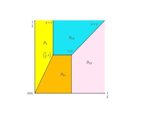
Figure 5: For Step 4 in the proof of Theorem 5.1.

Step 4. Let $\big{(}\frac{1}{p},\frac{1}{q}\big{)}\in\big{\{}\big{(}\frac{1}{p},\frac{1}{q}\big{)}\in\mbox{D}_{1}:\frac{1}{q}<1\big{\}}$. It is easy to see that $\big{(}\frac{1}{p},\frac{1}{q}\big{)}$ is a point at the line segment connecting $\big{(}\frac{1}{p}+\frac{1}{2}\big{(}1-\frac{1}{q}\big{)},1\big{)}$ and $\big{(}0,\frac{1}{q}-\frac{2}{p}\big{)}$, which is parallel to the line connecting $\big{(}\frac{1}{2},1\big{)}$ and $(0,0)$. At the point $(\frac{1}{\bar{p}},1):=\big{(}\frac{1}{p}+\frac{1}{2}\big{(}1-\frac{1}{q}\big{)},1\big{)}$, in Step 1 we have shown that $M^{s,\alpha}_{\bar{p},1}$ is a multiplication algebra if $s\geqslant n\alpha\big{[}\frac{1}{p}+\frac{1}{2}\big{(}1-\frac{1}{q}\big{)}\big{]}+\frac{n\alpha(1-\alpha)}{2-\alpha}\big{(}\frac{1}{q}-\frac{2}{p}\big{)}$. For $(0,\frac{1}{\bar{q}}):=\big{(}0,\frac{1}{q}-\frac{2}{p}\big{)}$, complex interpolation between $(0,1)$ in Step 1 and $(0,0)$ in Step 3 shows that once $s>n(1-\alpha)\big{(}1-\frac{1}{q}+\frac{2}{p}\big{)}+\frac{n\alpha(1-\alpha)}{2-\alpha}\big{(}\frac{1}{q}-\frac{2}{p}\big{)}$, the associated $\alpha$-modulation space $M^{s,\alpha}_{\infty,\bar{q}}$ is a multiplication algebra. Again, using the complex interpolation and combining the result in Step 2, and we arrive at (5.1) in $\mbox{D}_{1}$. Denote (see Fig. 5)

$$\begin{split}\mbox{D}_{21}&=[0,1]\times[0,1]\backslash\mbox{D}_{1};\\ \mbox{D}_{23}&=\left\{\big{(}\tfrac{1}{p},\tfrac{1}{q}\big{)}\in\mathbb{R}_{+}^{2}:\tfrac{1}{q}\geqslant\tfrac{1}{p}\right\}\Big{\backslash}\mbox{D}_{1}\cup\mbox{D}_{21}.\end{split}$$

Through the point $\big{(}\frac{1}{p},\frac{1}{q}\big{)}\in\mbox{D}_{21}$, one can make a line segment connecting $\big{(}\frac{1}{2q},\frac{1}{q}\big{)}$ and $\big{(}1,\frac{1}{q}\big{)}$. For $\big{(}\frac{1}{2q},\frac{1}{q}\big{)}$, we see that once $s>\frac{n\alpha}{2q}+n(1-\alpha)\big{(}1-\frac{1}{q}\big{)}$, $M_{2q,q}^{s,\alpha}$ is a multiplication algebra. For $\big{(}1,\frac{1}{q}\big{)}$, complex interpolation between $(1,1)$ in Step 1 and $(1,0)$ in Step 3 shows that once $s>n\alpha+n(1-\alpha)\big{(}1-\frac{1}{q}\big{)}$, the associated $\alpha$-modulation space is a multiplication algebra. Then we use complex interpolation to get that $M_{p,q}^{s,\alpha}$ is a multiplication algebra if $s>\frac{n\alpha}{p}+n(1-\alpha)\big{(}1-\frac{1}{q}\big{)}$. If $(1/p,1/q)\in\mbox{D}_{23}$, the result can be derived in a similar way.

If $\big{(}\frac{1}{p},\frac{1}{q}\big{)}\in\mbox{D}_{22}$, then it belongs to the segment by connecting $\big{(}\frac{1}{p},0\big{)}$ and $\big{(}\frac{1}{p},\frac{1}{p}\big{)}$. In Step 4 we see that once $s\geqslant\frac{n\alpha}{p}+n(1-\alpha)\frac{1}{p}+\frac{n\alpha(1-\alpha)}{2-\alpha}\big{(}\frac{1}{p}-1\big{)}$, $M_{p,\infty}^{s,\alpha}$ is a multiplication algebra; and once $s\geqslant\frac{n\alpha}{p}+\frac{n\alpha(1-\alpha)}{2-\alpha}\big{(}\frac{1}{p}-1\big{)}$, $M_{p,p}^{s,\alpha}$ is a multiplication algebra. Then complex interpolation between them gives once $s\geqslant\frac{n\alpha}{p}+n(1-\alpha)\big{(}\frac{1}{p}-\frac{1}{q}\big{)}+\frac{n\alpha(1-\alpha)}{2-\alpha}\big{(}\frac{1}{p}-1\big{)}$, $M_{p,q}^{s,\alpha}$ is a multiplication algebra. MM $\square$

6 Sharpness for the scaling and embedding properties

In this section we show the necessity of Theorems 3.1, 4.1 and 4.2. Since the $p$-$BAPU$ has no scaling, it is difficult to calculate the norm for a known function. However, we have the following equivalent norm on $\alpha$-modulation spaces. Let $\rho$ be a smooth radial bump function supported in $B(0,2)$, satisfying $\rho(\xi)=1$ as $|\xi|<1$, and $\rho(\xi)=0$ as $|\xi|\geqslant 2$. Let $\rho^{\alpha}_{k}$ be as in (1.4):

$$\rho^{\alpha}_{k}(\xi)=\rho\left(\frac{\xi-\langle k\rangle^{\alpha/(1-\alpha)}k}{C\langle k\rangle^{\alpha/(1-\alpha)}}\right).$$

Proposition 6.1.

Let $\rho^{\alpha}_{k}$ be as in the above. Then

$$\|f\|^{\circ}_{M^{s,\alpha}_{p,q}}=\left(\sum_{k\in\mathbb{Z}^{n}}\langle k\rangle^{\frac{sq}{1-\alpha}}\|(\mathscr{F}^{-1}\rho^{\alpha}_{k})*f\|^{q}_{p}\right)^{1/q}$$

is an equivalent norm on $M^{s,\alpha}_{p,q}$.

Proof.

If $p\geq 1$, in view of Young’s inequality,

$$\|(\mathscr{F}^{-1}\rho^{\alpha}_{k})*f\|_{p}\leq\sum_{|\ell|_{\infty}\leq C}\|(\mathscr{F}^{-1}\rho^{\alpha}_{k+\ell})\|_{1}\|\Box^{\alpha}_{k}f\|_{p}\lesssim\|\Box^{\alpha}_{k}f\|_{p}.$$

If $p<1$, by Proposition 2.1 and the scaling argument, we have

$$\|(\mathscr{F}^{-1}\rho^{\alpha}_{k})*f\|_{p}\leq\langle k\rangle^{n\alpha(1/p-1)/(1-\alpha)}\sum_{|\ell|_{\infty}\leq C}\|(\mathscr{F}^{-1}\rho^{\alpha}_{k+\ell})\|_{p}\|\Box^{\alpha}_{k}f\|_{p}\lesssim\|\Box^{\alpha}_{k}f\|_{p}.$$

Combining the above two cases, we have $\|f\|^{\circ}_{M^{s,\alpha}_{p,q}}\leq\|f\|_{M^{s,\alpha}_{p,q}}$. On the other hand, noticing that

$$\eta^{\alpha}_{k}=\rho^{\alpha}_{k}\frac{\rho\left(\frac{\xi-\langle k\rangle^{\alpha/(1-\alpha)}k}{2C\langle k\rangle^{\alpha/(1-\alpha)}}\right)}{\sum_{\ell\in\mathbb{Z}^{n}}\rho\left(\frac{\xi-\langle k+\ell\rangle^{\alpha/(1-\alpha)}(k+\ell)}{C\langle k+\ell\rangle^{\alpha/(1-\alpha)}}\right)}:=\rho^{\alpha}_{k}\sigma^{\alpha}_{k},$$

We have for $p\geq 1$, in view of Young’s inequality,

$$\|\Box^{\alpha}_{k}f\|_{p}\leq\|(\mathscr{F}^{-1}\rho^{\alpha}_{k})*f\|_{p}\|(\mathscr{F}^{-1}\sigma^{\alpha}_{k})\|_{1}\lesssim\|(\mathscr{F}^{-1}\rho^{\alpha}_{k})*f\|_{p}.$$

If $p<1$, by Proposition 2.1, the scaling argument and the generalized Bernstein inequality, we have

$$\|\Box^{\alpha}_{k}f\|_{p}\lesssim\langle k\rangle^{n\alpha(1/p-1)/(1-\alpha)}\|(\mathscr{F}^{-1}\rho^{\alpha}_{k})*f\|_{p}\|\mathscr{F}^{-1}\sigma^{\alpha}_{k}\|_{p}\|\Box^{\alpha}_{k}f\|_{p}\lesssim\|(\mathscr{F}^{-1}\rho^{\alpha}_{k})*f\|_{p}.$$

The result follows. MM $\square$

Proof of Theorem 3.1.

(Necessity) We divide the proof into the following two cases $\lambda\gg 1$ and $\lambda\ll 1$, respectively.

Case 1. $\lambda\gg 1$. One needs to show that

$$\|f_{\lambda}\|_{M_{p,q}^{s,\alpha}}\gtrsim\lambda^{-\frac{n}{p}+n\big{(}\frac{1}{p}-1\big{)}\vee(s+s_{c})}\|f\|_{M_{p,q}^{s,\alpha}}.$$

Case 1.1. We consider the case $s_{p}=n(1/p-1)>s+s_{c}$. Our aim is to show that there exists a function $f$ satisfying

$$\|f_{\lambda}\|_{M_{p,q}^{s,\alpha}}\gtrsim\lambda^{-n}\|f\|_{M_{p,q}^{s,\alpha}}.$$

Taking $f=\mathscr{F}^{-1}\rho$, we have

$$\begin{split}\|f_{\lambda}\|^{\circ}_{M_{p,q}^{s,\alpha}}\geq\|(\mathscr{F}^{-1}\rho^{\alpha}_{0})*f_{\lambda}\|_{p}\geqslant\lambda^{-n}\|\mathscr{F}^{-1}\rho\|_{p}\gtrsim\lambda^{-n}\|f\|_{M_{p,q}^{s,\alpha}}.\end{split}$$ (6.1)

Case 1.2. We consider the case $s_{p}<s+s_{c}$. According to the definition of $s_{c}$, we separate the proof into the following three cases.

Case 1.2.1. $s_{c}=n(1-\alpha)(1/p+1/q-1)$. Put $f=\mathscr{F}^{-1}\rho$. Since $\lambda\gg 1$, we see that for some $0<\varepsilon_{0}<\varepsilon_{1}\ll 1$,

$$(\mathscr{F}^{-1}\rho^{\alpha}_{k})*f_{\lambda}=\lambda^{-n}\mathscr{F}^{-1}\rho^{\alpha}_{k},\quad\quad|k|\in[\varepsilon_{0}\lambda^{1-\alpha},\ \varepsilon_{1}\lambda^{1-\alpha}].$$

It follows that

$$\begin{split}\|f_{\lambda}\|^{\circ}_{M_{p,q}^{s,\alpha}}&\gtrsim\lambda^{-n}\left(\sum_{|l|\in[\varepsilon_{0}\lambda^{1-\alpha},\ \varepsilon_{1}\lambda^{1-\alpha}]}\langle l\rangle^{\frac{sq}{1-\alpha}}\|\mathscr{F}^{-1}\rho_{l}^{\alpha}\|_{p}^{q}\right)^{\frac{1}{q}}\\ &\gtrsim\lambda^{-\frac{n}{p}+s+n(1-\alpha)\big{(}\frac{1}{p}+\frac{1}{q}-1\big{)}}\\ &\gtrsim\lambda^{-\frac{n}{p}+s+n(1-\alpha)\big{(}\frac{1}{p}+\frac{1}{q}-1\big{)}}\|f\|_{M_{p,q}^{s,\alpha}}.\end{split}$$ (6.2)

Case 1.2.2. $s_{c}=0$. Let us take $f={\rm e}^{{\rm i}x_{1}}\mathscr{F}^{-1}\rho_{\lambda}.$ We have $f_{\lambda}=\lambda^{-n}e^{{\rm i}x_{1}\lambda}\mathscr{F}^{-1}\rho$. We may assume that there exists $l_{0}\in\mathbb{N}$ such that $\langle l_{0}\rangle^{\alpha/(1-\alpha)}l_{0}\sim\lambda$ and $B((\lambda,0,...,0),\ 2)\subset B(\langle l_{0}\rangle^{\alpha/(1-\alpha)}(l_{0},0,...,0),\ C\langle l_{0}\rangle^{\alpha/(1-\alpha)})$. It is easy to see that $\|f\|_{p}\sim\lambda^{n\big{(}\frac{1}{p}-1\big{)}}$ and

$$\|f_{\lambda}\|_{M_{p,q}^{s,\alpha}}\sim\lambda^{-n}\langle l_{0}\rangle^{s/(1-\alpha)}\sim\lambda^{-n+s}\gtrsim\lambda^{-\frac{n}{p}+s}\|f\|_{p}\gtrsim\lambda^{-\frac{n}{p}+s}\|f\|_{M_{p,q}^{s,\alpha}}.$$ (6.3)

Case 1.2.3. $s_{c}=n(1-\alpha)(1/q-1/p)$. Put

$$f^{(l)}={\rm e}^{{\rm i}x\langle l\rangle^{\frac{\alpha}{1-\alpha}}l/\lambda}\ \tau_{\lambda^{1-\alpha}l}\left(\rho\left(\frac{\lambda\ \cdot}{c\langle l\rangle^{\frac{\alpha}{1-\alpha}}}\right)\right)^{\vee},\quad f=\sum_{|\ell|\sim\lambda^{1-\alpha}}f^{(l)},$$ (6.4)

where $|\ell|\sim\lambda^{1-\alpha}$ means that $|l|\in[\varepsilon_{0}\lambda^{1-\alpha},\ \varepsilon_{1}\lambda^{1-\alpha}]$ for some $0<\varepsilon_{0}<\varepsilon_{1}\ll 1.$ If $|l|\sim\lambda^{1-\alpha}$, then $\|f^{(l)}\|_{p}\sim\lambda^{n(1-\alpha)\big{(}\frac{1}{p}-1\big{)}}$, and

$$(f^{(l)})_{\lambda}={\rm e}^{{\rm i}x\langle l\rangle^{\frac{\alpha}{1-\alpha}}l}\ \tau_{\lambda^{1-\alpha}l}\left(\rho\left(\frac{\cdot}{c\langle l\rangle^{\frac{\alpha}{1-\alpha}}}\right)\right)^{\vee},$$ (6.5)

which follows that $(\mathscr{F}^{-1}\rho^{\alpha}_{l})*(f^{(l)})_{\lambda}=(f^{(l)})_{\lambda}$. Since supp $\rho^{\alpha}_{l}$ overlaps at most finite many supp $\rho^{\alpha}_{l+k}$, we see that $\Box^{\alpha}_{l+k}(f^{(l)})_{\lambda}=0$ if $|k|\geq C$. Let $A(\lambda)\subset\{l:|l|\sim\lambda^{1-\alpha}\}$ be the set so that for any $l,\tilde{l}\in A(\lambda)$ ($l\neq\tilde{l}$), $|l-\tilde{l}|\geq C$. We have

$$\begin{split}\left\|f_{\lambda}\right\|_{M_{p,q}^{s,\alpha}}&\gtrsim\left(\sum_{l\in A{(\lambda)}}\langle l\rangle^{\frac{sq}{1-\alpha}}\|(f^{(l)})_{\lambda}\|_{p}^{q}\right)^{\frac{1}{q}}\\ &\gtrsim\lambda^{-\frac{n}{p}+s}\left(\sum_{l\in A{(\lambda)}}\|f^{(l)}\|_{p}^{q}\right)^{\frac{1}{q}}\\ &\gtrsim\lambda^{-\frac{n}{p}+s+n(1-\alpha)\big{(}\frac{1}{q}+\frac{1}{p}-1\big{)}}.\end{split}$$ (6.6)

Moreover, we easily see that

$$|\widehat{f}^{(l)}(\xi)|=\rho\left(\frac{\lambda\xi-\langle l\rangle^{\alpha/(1-\alpha)}l}{c\langle l\rangle^{\alpha/(1-\alpha)}}\right).$$

It follows that ${\rm supp}\ \widehat{f}^{(l)}$ is included in the unit ball. Hence, we have

$$\left\|f\right\|_{M_{p,q}^{s,\alpha}}\lesssim\left\|\sum_{l\in A{(\lambda)}}f^{(l)}\right\|_{p}.$$

By Plancheral’s identity,

$$\left\|f\right\|_{2}=\left\|\widehat{f}\right\|_{2}=\left(\sum_{l\in A{(\lambda)}}\int\rho^{2}\left(\frac{\lambda\xi-\langle l\rangle^{\alpha/(1-\alpha)}l}{c\langle l\rangle^{\alpha/(1-\alpha)}}\right)d\xi\right)^{1/2}\sim 1.$$

On the other hand, in view of $\mathscr{F}^{-1}\rho$ is a Schwartz function, we have

$$|\mathscr{F}^{-1}\rho(x)|\lesssim\langle x\rangle^{-N}.$$

It follows that for $N\gg n$,

$$\left|\sum_{l\in A{(\lambda)}}f^{(l)}(x)\right|\lesssim\lambda^{-n(1-\alpha)}\sum_{l\in A{(\lambda)}}\left(1+\lambda^{-(1-\alpha)}|x-\lambda^{1-\alpha}l|\right)^{-N}\lesssim\lambda^{-n(1-\alpha)}.$$

By Hölder’s inequality,

$$\left\|f\right\|_{M_{p,q}^{s,\alpha}}\lesssim\left\|f\right\|_{p}\lesssim\lambda^{n(1-\alpha)(2/p-1)}.$$

The result follows.

Case 2. $\lambda\ll 1$. It suffices to show that for some $f\in M^{s,\alpha}_{p,q}$,

$$\|f_{\lambda}\|^{\circ}_{M_{p,q}^{s,\alpha}}\gtrsim\lambda^{-\frac{n}{p}}(1\vee\lambda^{s+s_{c}})\|f\|_{M_{p,q}^{s,\alpha}}.$$

Case 2.1. $s+s_{c}\geq 0$. Taking $f=\mathscr{F}^{-1}\rho$, we have

$$\|f_{\lambda}\|^{\circ}_{M_{p,q}^{s,\alpha}}=\|(\mathscr{F}^{-1}\rho)(\lambda\,\cdot)\|_{p}\sim\lambda^{-\frac{n}{p}}\|f\|_{M_{p,q}^{s,\alpha}}.$$ (6.7)

Case 2.2. $s+s_{c}<0$. We divide the proof into the following three cases.

Case 2.2.1. We can find some $k_{0}$ such that $\lambda\langle k_{0}\rangle^{\frac{1}{1-\alpha}}\sim 1$. Denote

$$f={\rm e}^{{\rm i}x\langle k_{0}\rangle^{\frac{\alpha}{1-\alpha}}k_{0}}\mathscr{F}^{-1}\left(\rho\left(\frac{\cdot}{c\langle k_{0}\rangle^{\frac{\alpha}{1-\alpha}}}\right)\right),$$ (6.8)

We have

$$\widehat{f}_{\lambda}=\lambda^{-n}\rho\left(\frac{\xi/\lambda-\langle k_{0}\rangle^{\frac{\alpha}{1-\alpha}}k_{0}}{c\langle k_{0}\rangle^{\frac{\alpha}{1-\alpha}}}\right),$$ (6.9)

Therefore,

$$\|f_{\lambda}\|^{\circ}_{M_{p,q}^{s,\alpha}}\gtrsim\|f_{\lambda}\|_{p}\gtrsim\lambda^{-\frac{n}{p}+s}\langle k_{0}\rangle^{\frac{s}{1-\alpha}}\|f\|_{p}\gtrsim\lambda^{-\frac{n}{p}+s}\|f\|_{M_{p,q}^{s,\alpha}}.$$ (6.10)

Case 2.2.2. Taking $f=\lambda^{n}\mathscr{F}^{-1}\rho_{\lambda}$, we have $f_{\lambda}=\mathscr{F}^{-1}\rho$. It follows that $\|f_{\lambda}\|^{\circ}_{M_{p,q}^{s,\alpha}}\sim 1$. On the other hand,

$$\begin{split}\|f\|^{\circ}_{M_{p,q}^{s,\alpha}}&\lesssim\left(\sum_{|k|\lesssim\lambda^{\alpha-1}}\langle k\rangle^{\frac{sq}{1-\alpha}}\|(\mathscr{F}^{-1}\rho_{k}^{\alpha})*f\|_{p}^{q}\right)^{\frac{1}{q}}\\ &\lesssim\left(\sum_{|k|\lesssim\lambda^{\alpha-1}}\langle k\rangle^{\frac{sq}{1-\alpha}}\|\mathscr{F}^{-1}\rho_{k}^{\alpha})\|^{q}_{p}\|f\|_{1}^{q}\right)^{\frac{1}{q}}\\ &\lesssim\lambda^{n-s-n(1-\alpha)\frac{1}{q}-n\alpha\big{(}1-\frac{1}{p}\big{)}}.\end{split}$$ (6.11)

It follows that

$$\|f_{\lambda}\|^{\circ}_{M_{p,q}^{s,\alpha}}\gtrsim\lambda^{-\frac{n}{p}+s+s_{c}}\|f\|_{M_{p,q}^{s,\alpha}}.$$

Case 2.2.3. $s_{c}=n(1-\alpha)(1/q-1/p)$. Let $A(\lambda)$ be the set so that for any $l,\tilde{l}\in A(\lambda)$ ($l\neq\tilde{l}$), $|l-\tilde{l}|\geq C$ and $|l|\in[\varepsilon_{0}\lambda^{\alpha-1},\ \varepsilon_{1}\lambda^{\alpha-1}]$ for some $0<\varepsilon_{0}<\varepsilon_{1}\ll 1$. Take

$$f^{(l)}={\rm e}^{{\rm i}x\langle l\rangle^{\frac{\alpha}{1-\alpha}}l}\tau_{C^{\prime}l}\mathscr{F}^{-1}\left(\rho\left(\frac{\cdot}{c\langle l\rangle^{\frac{\alpha}{1-\alpha}}}\right)\right),\ \ f=\sum_{l\in A(\lambda)}f^{(l)}.$$ (6.12)

One easily sees that

$$(f^{(l)})_{\lambda}=\lambda^{-n}{\rm e}^{{\rm i}x\lambda\langle l\rangle^{\frac{\alpha}{1-\alpha}}l}\tau_{C^{\prime}l}\mathscr{F}^{-1}\left(\rho\left(\frac{\cdot}{c\lambda\langle l\rangle^{\frac{\alpha}{1-\alpha}}}\right)\right).$$ (6.13)

We have

$$\begin{split}\left\|f\right\|^{\circ}_{M_{p,q}^{s,\alpha}}&=\left(\sum_{l\in A{(\lambda)}}\langle l\rangle^{\frac{sq}{1-\alpha}}\|(f^{(l)})\|_{p}^{q}\right)^{\frac{1}{q}}\\ &\lesssim\lambda^{-s}\left(\sum_{l\in A{(\lambda)}}\langle l\rangle^{\frac{n\alpha}{1-\alpha}(1-\frac{1}{p})q}\right)^{\frac{1}{q}}\\ &\lesssim\lambda^{-s+n\alpha\big{(}\frac{1}{p}-1\big{)}+\frac{n(\alpha-1)}{q}}.\end{split}$$ (6.14)

Since ${\rm supp}\widehat{f}^{(l)}_{\lambda}$ is contained in the unit ball, we see that

$$\left\|f_{\lambda}\right\|_{M_{p,q}^{s,\alpha}}\gtrsim\left\|\sum_{l\in A{(\lambda)}}{f}^{(l)}_{\lambda}\right\|_{p}=\lambda^{-n/p}\left\|\sum_{l\in A{(\lambda)}}{f}^{(l)}\right\|_{p}.$$

We note that

$$f^{(l)}(x)=\langle l\rangle^{\frac{n\alpha}{1-\alpha}}{\rm e}^{{\rm i}x\langle l\rangle^{\frac{\alpha}{1-\alpha}}l}(\mathscr{F}^{-1}\rho)\left(c\langle l\rangle^{\frac{\alpha}{1-\alpha}}(x-C^{\prime}l)\right).$$

Due to $\mathscr{F}^{-1}\rho$ is a Schwartz function, we see that $|\mathscr{F}^{-1}\rho(x)|\lesssim\langle x\rangle^{-2n}$. We can assume that $\mathscr{F}^{-1}\rho(0)=1$, which follows that there exists a $\delta>0$ such that

$$|\mathscr{F}^{-1}\rho(x)|\geq 1/2,\quad|x|\leq\delta.$$

Hence, for any $k\in A(\lambda)$, $x\in B(C^{\prime}k,\delta/c\langle k\rangle^{\frac{\alpha}{1-\alpha}})$,

$$\left|\sum_{l\in A(\lambda)}f^{(l)}(x)\right|\geq\frac{\lambda^{-n\alpha}}{2}-C\lambda^{-n\alpha}\sup_{|y|\lesssim\delta}\sum_{l\in\mathbb{Z}^{n}}\left(y+C^{\prime}c\ l\right)^{-2n}.$$

We can take $C^{\prime}c\gg 1$. It follows that for any $k\in A(\lambda)$,

$$\left|\sum_{l\in A(\lambda)}f^{(l)}(x)\right|\geq\frac{\lambda^{-n\alpha}}{2}-C\lambda^{-n\alpha}(C^{\prime}c)^{-n}\geq\frac{\lambda^{-n\alpha}}{4},\quad x\in B(C^{\prime}k,\delta/c\langle k\rangle^{\frac{\alpha}{1-\alpha}}).$$

So, we have

$$\left\|\sum_{l\in A(\lambda)}f^{(l)}(x)\right\|_{p}\gtrsim\lambda^{-n\alpha}\lambda^{\frac{2n\alpha-n}{p}}.$$

It follows that

$$\|f_{\lambda}\|^{\circ}_{M_{p,q}^{s,\alpha}}\gtrsim\lambda^{-n/p+s+n(1-\alpha)(1/q-1/p)}\|f\|_{M_{p,q}^{s,\alpha}}.$$

The result follows. MM $\square$

Proof of Theorem 4.2.

(Necessity) Case 1. Let us assume that $B^{s_{1}}_{p,q}\subset M^{s_{2}}_{p,q}$.

Case 1.1. We show that $s_{1}\geq s_{2}$. Let $k\in\mathbb{Z}^{n}$, $|k|\gg 1$ with $B(\langle k\rangle^{\frac{\alpha}{1-\alpha}}k,C\langle k\rangle^{\frac{\alpha}{1-\alpha}})\subset\{\xi:\ 5\cdot 2^{j-3}\leq|\xi|\leq 3\cdot 2^{j-1}\}$. We see that

$$\left\|\mathscr{F}^{-1}\left(\rho_{k}^{\alpha}(2\ \cdot)\right)\right\|^{\circ}_{M_{p,q}^{s_{2},\alpha}}\geqslant\langle k\rangle^{\frac{s_{2}}{1-\alpha}}\|\mathscr{F}^{-1}\rho_{k}^{\alpha}(2\ \cdot)\|_{p}\gtrsim\langle k\rangle^{\frac{s_{2}}{1-\alpha}+\frac{n\alpha}{1-\alpha}\big{(}1-\frac{1}{p}\big{)}},$$

$$\left\|\mathscr{F}^{-1}\left(\rho_{k}^{\alpha}(2\ \cdot)\right)\right\|_{B_{p,q}^{s_{1}}}\leqslant 2^{js_{1}}\|\mathscr{F}^{-1}\rho_{k}^{\alpha}(2\ \cdot)\|_{p}\lesssim\langle k\rangle^{\frac{s_{1}}{1-\alpha}+\frac{n\alpha}{1-\alpha}\big{(}1-\frac{1}{p}\big{)}}.$$

$B_{p,q}^{s_{1}}\subset M_{p,q}^{s_{2},\alpha}$ follows that $s_{1}\geqslant s_{2}$.

Case 1.2. We show that $s_{1}\geq s_{2}+n(1-\alpha)(1/p+1/q-1)$. One has that

$$\|\mathscr{F}^{-1}\varphi_{j}\|_{B_{p,q}^{s_{1}}}\lesssim 2^{js_{1}+jn\big{(}1-\frac{1}{p}\big{)}}.$$ (6.15)

Denote

$$A_{j}=\{k:\ {\rm supp}\rho_{k}^{\alpha}\subset\{\xi:\ 5\cdot 2^{j-3}\leq|\xi|\leq 3\cdot 2^{j-1}\}\}.$$

$$\|\mathscr{F}^{-1}\varphi_{j}\|^{\circ}_{M_{p,q}^{s_{2},\alpha}}\geqslant\left(\sum_{k\in A_{j}}\langle k\rangle^{\frac{s_{2}q}{1-\alpha}}\|\mathscr{F}^{-1}\rho_{k}^{\alpha}\|_{p}^{q}\right)^{\frac{1}{q}}\gtrsim\left(\sum_{k\in A_{j}}\langle k\rangle^{\frac{s_{2}q}{1-\alpha}+\frac{n\alpha}{1-\alpha}\big{(}1-\frac{1}{p}\big{)}q}\right)^{\frac{1}{q}}.$$ (6.16)

Noticing that $\#A_{j}\sim O(2^{nj(1-\alpha)})$, we immediately have

$$\|\mathscr{F}^{-1}\varphi_{j}\|^{\circ}_{M_{p,q}^{s_{2},\alpha}}\gtrsim 2^{s_{2}j+n\alpha j\big{(}1-\frac{1}{p}\big{)}+n(1-\alpha)j\frac{1}{q}}.$$ (6.17)

$B_{p,q}^{s_{1}}\subset M_{p,q}^{s_{2},\alpha}$ implies that $s_{1}\geqslant s_{2}+n(1-\alpha)\big{(}\frac{1}{p}+\frac{1}{q}-1\big{)}$.

Case 1.3. We show that $s_{1}\geqslant s_{2}+n(1-\alpha)\big{(}\frac{1}{q}-\frac{1}{p}\big{)}$. We denote by $A_{j}$ the set such that for every $k,l\in\mathbb{Z}^{n}\cap A_{j}$ ($l\neq\tilde{l}$), $|k-l|\geq C$ and $|k|^{1/(1-\alpha)}\in[5\cdot 2^{j-3}+C2^{j\alpha},3\cdot 2^{j-1}-C2^{j\alpha}]$. Put

$$f^{(k)}=\tau_{k}\left(\mathscr{F}^{-1}\rho_{k}^{\alpha}\right),\quad\quad f=\sum_{k\in A_{j}}f^{(k)}.$$ (6.18)

Noticing that $\#A_{j}\sim O(2^{nj(1-\alpha)})$, we have

$$\left\|f\right\|^{\circ}_{M_{p,q}^{s_{2},\alpha}}=\left(\sum_{k\in A_{j}}\langle k\rangle^{\frac{s_{2}q}{1-\alpha}}\|f^{(k)}\|_{p}^{q}\right)^{\frac{1}{q}}\gtrsim 2^{j\left(s_{2}+n(1-\alpha)\frac{1}{q}+n\alpha\big{(}1-\frac{1}{p}\big{)}\right)}.$$ (6.19)

On the other hand,

$$\left\|f\right\|_{B_{p,q}^{s_{1}}}\lesssim 2^{js_{1}}\left\|\sum_{k\in A_{j}}f^{(k)}\right\|_{p}.$$ (6.20)

By Plancherel’s identity,

$$\|f\|_{2}\lesssim\left(\sum_{k\in A_{j}}\|\rho^{\alpha}_{k}(2\ \cdot)\|^{2}_{2}\right)^{1/2}\lesssim 2^{nj/2}.$$

Moreover, let us observe that

$$f^{(k)}=C\langle k\rangle^{\frac{n\alpha}{1-\alpha}}(\mathscr{F}^{-1}\rho)(C\langle k\rangle^{\frac{n\alpha}{1-\alpha}}(x-k)).$$

Using the same way as in the proof of Case 1.2.3 in Theorem 3.1, we have

$$|f(x)|\lesssim 2^{n\alpha j}.$$

By Hölder’s inequality,

$$\|f\|_{p}\lesssim 2^{jn\alpha(1-2/p)+nj/p}.$$

It follows from $B_{p,q}^{s_{1}}\subset M_{p,q}^{s_{2},\alpha}$ that $s_{1}\geqslant s_{2}+n(1-\alpha)\big{(}\frac{1}{q}-\frac{1}{p}\big{)}$.

Case 2. We assume that $M_{p,q}^{s_{1},\alpha_{1}}\subset B_{p,q}^{s_{2}}$.

Case 2.1. Let $j\gg 1$. One can find some $k\in\mathbb{Z}^{n}$ verifying $\rho_{k}^{\alpha}\varphi_{j}=\rho_{k}^{\alpha}$. It follows that $2^{j}\sim\langle k\rangle^{1/(1-\alpha)}$. Thus,

$$\|\mathscr{F}^{-1}\rho_{k}^{\alpha}\|_{B_{p,q}^{s_{2}}}\geqslant 2^{js_{2}}\|\mathscr{F}^{-1}\rho_{k}^{\alpha}\|_{p}\gtrsim 2^{js_{2}}\langle k\rangle^{\frac{n\alpha}{1-\alpha}\big{(}1-\frac{1}{p}\big{)}},$$ (6.21)

$$\|\mathscr{F}^{-1}\rho_{k}^{\alpha}\|^{\circ}_{M_{p,q}^{s_{1},\alpha}}\lesssim\langle k\rangle^{\frac{s_{1}}{1-\alpha}+\frac{n\alpha}{1-\alpha}\big{(}1-\frac{1}{p}\big{)}}.$$ (6.22)

So, we have $s_{1}\geqslant s_{2}$.

Case 2.2. Let $j\gg 1$. We have

$$\left\|\mathscr{F}^{-1}\varphi_{j}\right\|_{B_{p,q}^{s_{2}}}\geqslant 2^{js_{2}}\|\mathscr{F}^{-1}\varphi^{2}_{j}\|_{p}\gtrsim 2^{js_{2}+jn\big{(}1-\frac{1}{p}\big{)}}.$$ (6.23)

On the other hand,

$$\left\|\mathscr{F}^{-1}\varphi_{j}\right\|_{M_{p,q}^{s_{1},\alpha}}\lesssim\left(\sum_{|k|^{1/(1-\alpha)}\sim 2^{j}}\langle k\rangle^{\frac{s_{1}q}{1-\alpha}}2^{jn\alpha\big{(}1-\frac{1}{p}\big{)}q}\right)^{\frac{1}{q}}\lesssim 2^{jn(1-\alpha)\frac{1}{q}+s_{1}j+jn\alpha\big{(}1-\frac{1}{p}\big{)}}.$$ (6.24)

It follows from $M_{p,q}^{s_{1},\alpha}\subset B_{p,q}^{s_{2}}$ that $s_{1}\geqslant s_{2}+n(1-\alpha)\big{(}1-\frac{1}{p}-\frac{1}{q}\big{)}$.

Case 2.3. We denote by $A_{j}$ the set such that for every $k,l\in\mathbb{Z}^{n}\cap A_{j}$ ($l\neq k$), $|k-l|\geq C$ and $|k|^{1/(1-\alpha)}\in[5\cdot 2^{j-3}+C2^{j\alpha},\ 3\cdot 2^{j-1}-C2^{j\alpha}]$. Put

$$f^{(k)}=\tau_{C^{\prime}k}\mathscr{F}^{-1}\left(\rho\left(\frac{\cdot\ -\langle k\rangle^{\frac{\alpha}{1-\alpha}}k}{c\langle k\rangle^{\frac{\alpha}{1-\alpha}}}\right)\right),\ \ f=\sum_{k\in A_{j}}f^{(k)}.$$ (6.25)

Using the same way as in the proof of Case 2.2.3 in Theorem 3.1,

$$\left\|f\right\|^{\circ}_{M_{p,q}^{s_{1},\alpha}}\lesssim 2^{j\left[s_{1}+n(1-\alpha)\frac{1}{q}+n\alpha\big{(}1-\frac{1}{p}\big{)}\right]},$$ (6.26)

$$\left\|f\right\|_{B_{p,q}^{s_{2}}}=2^{js_{2}}\left\|f\right\|_{p}\gtrsim 2^{j\left[s_{2}+n(1-\alpha)\frac{1}{p}+n\alpha\big{(}1-\frac{1}{p}\big{)}\right]}.$$ (6.27)

From $M_{p,q}^{s_{1},\alpha}\subset B_{p,q}^{s_{2}}$ it follows that $s_{1}\geqslant s_{2}+n(1-\alpha)\big{(}\frac{1}{p}-\frac{1}{q}\big{)}$. MM $\square$

Proof of Theorem 4.1.

(Necessity) We separate the proof into the following two cases.

Case 1. We assume that $M_{p,q}^{s_{1},\alpha_{1}}\subset M_{p,q}^{s_{2},\alpha_{2}}$ with $\alpha_{1}\geqslant\alpha_{2}$.

Case 1.1. We show that $s_{1}\geq s_{2}$. Denote

$$\Lambda_{2}(k)=\{l\in\mathbb{Z}^{n}:\ \rho^{\alpha_{2}}_{k}\rho^{\alpha_{1}}_{l}\neq 0\}.$$

We have

$$\left\|\mathscr{F}^{-1}\rho_{k}^{\alpha_{2}}\right\|^{\circ}_{M_{p,q}^{s_{2},\alpha_{2}}}\geqslant\langle k\rangle^{\frac{s_{2}}{1-\alpha_{2}}}\|\mathscr{F}^{-1}\rho_{k}^{\alpha_{2}}\rho^{\alpha_{2}}_{k}\|_{p}\gtrsim\langle k\rangle^{\frac{s_{2}}{1-\alpha_{2}}+\frac{n\alpha_{2}}{1-\alpha_{2}}\big{(}1-\frac{1}{p}\big{)}},$$ (6.28)

and

$$\left\|\mathscr{F}^{-1}\rho_{k}^{\alpha_{2}}\right\|^{\circ}_{M_{p,q}^{s_{1},\alpha_{1}}}\lesssim\left(\sum_{l\in\Lambda_{2}(k)}\langle l\rangle^{\frac{s_{1}q}{1-\alpha_{1}}}\|\mathscr{F}^{-1}\rho_{k}^{\alpha_{2}}\rho_{l}^{\alpha_{1}}\|^{q}_{p}\right)^{\frac{1}{q}}.$$ (6.29)

Using Young’s inequality and Proposition 2.1, respectively for $p\geq 1$ and $p<1$, we have

$$\|\mathscr{F}^{-1}\rho_{k}^{\alpha_{2}}\rho_{l}^{\alpha_{1}}\|_{p}\lesssim\|\mathscr{F}^{-1}\rho_{k}^{\alpha_{2}}\|_{p}\lesssim\langle k\rangle^{\frac{n\alpha_{2}}{1-\alpha_{2}}\big{(}1-\frac{1}{p}\big{)}}.$$

Since $\#\Lambda_{2}(k)$ is finite and $|k|^{\frac{1}{1-\alpha_{2}}}\sim|l|^{\frac{1}{1-\alpha_{1}}}$ for all $l\in\lambda_{2}(k)$, one has that

$$\left\|\mathscr{F}^{-1}\rho_{k}^{\alpha_{2}}\right\|^{\circ}_{M_{p,q}^{s_{1},\alpha_{1}}}\lesssim\left(\sum_{k\in\Lambda_{2}(k)}\langle k\rangle^{\frac{sq}{1-\alpha_{1}}}\langle k\rangle^{\frac{n\alpha_{2}}{1-\alpha_{2}}\big{(}1-\frac{1}{p}\big{)}q}\right)^{\frac{1}{q}}\lesssim\langle k\rangle^{\frac{s}{1-\alpha_{2}}+\frac{n\alpha_{2}}{1-\alpha_{2}}\big{(}1-\frac{1}{p}\big{)}}.$$ (6.30)

From $M_{p,q}^{s,\alpha_{1}}\subset M_{p,q}^{s_{2},\alpha_{2}}$ it follows that $s_{1}\geqslant s_{2}$.

Case 1.2. Let $k\in\mathbb{Z}^{n}$ with $|k|\gg 1$. Denote

$$\Lambda^{*}(k)=\left\{l\in\mathbb{Z}^{n}:\rho_{k}^{\alpha_{1}}\rho_{l}^{\alpha_{2}}=\rho_{l}^{\alpha_{2}}\right\}.$$ (6.31)

We have

$$\|\mathscr{F}^{-1}\rho_{k}^{\alpha_{1}}\|_{M_{p,q}^{s_{1},\alpha_{1}}}\lesssim\langle k\rangle^{\frac{s_{1}}{1-\alpha_{1}}+\frac{n\alpha_{1}}{1-\alpha_{1}}\big{(}1-\frac{1}{p}\big{)}}.$$ (6.32)

Since $\#\Lambda^{*}(k)\sim\langle k\rangle^{\frac{n(\alpha_{1}-\alpha_{2})}{1-\alpha_{1}}}$ and $\langle k\rangle^{\frac{1}{1-\alpha_{1}}}\sim\langle l\rangle^{\frac{1}{1-\alpha_{2}}}$ for all $l\in\Lambda^{*}(k)$, one has that

$$\|\mathscr{F}^{-1}\rho_{k}^{\alpha_{1}}\|^{\circ}_{M_{p,q}^{s_{2},\alpha_{2}}}\geqslant\left(\sum_{l\in\Lambda^{*}(k)}\langle l\rangle^{\frac{s_{2}q}{1-\alpha_{2}}}\|\mathscr{F}^{-1}\eta_{l}^{\alpha_{2}}\|_{p}^{q}\right)^{\frac{1}{q}}\gtrsim\langle k\rangle^{\frac{n(\alpha_{1}-\alpha_{2})}{q(1-\alpha_{1})}+\frac{s_{2}}{1-\alpha_{1}}+\frac{n\alpha_{2}}{1-\alpha_{1}}\big{(}1-\frac{1}{p}\big{)}}.$$ (6.33)

$M_{p,q}^{s,\alpha_{1}}\subset M_{p,q}^{s_{2},\alpha_{2}}$ implies that $s_{1}\geqslant s_{2}+n(\alpha_{1}-\alpha_{2})\big{(}\frac{1}{p}+\frac{1}{q}-1\big{)}$.

Case 1.3. We show that $s_{1}\geqslant s_{2}+n(\alpha_{1}-\alpha_{2})\big{(}\frac{1}{q}-\frac{1}{p}\big{)}$. Let $\Lambda^{*}_{0}(k)$ be the subset of $\Lambda^{*}(k)$ such that $|l-\tilde{l}|\geq C$ for all $l,\tilde{l}\in\Lambda^{*}_{0}(k)$ ($l\neq\tilde{l}$). Denote

$$f^{(l)}=\tau_{l}\mathscr{F}^{-1}\rho^{\alpha_{2}}_{l},\quad\quad f=\sum_{l\in\Lambda^{*}_{0}(k)}f^{(l)}.$$ (6.34)

It follows that

$$\left\|f\right\|^{\circ}_{M_{p,q}^{s_{2},\alpha_{2}}}=\left(\sum_{l\in\Lambda^{*}_{0}(k)}\langle l\rangle^{\frac{s_{2}q}{1-\alpha_{2}}}\|f^{(l)}\|_{p}^{q}\right)^{\frac{1}{q}}\gtrsim\langle k\rangle^{\frac{s_{2}}{1-\alpha_{1}}+\frac{n(\alpha_{1}-\alpha_{2})}{q(1-\alpha_{1})}+\frac{n\alpha_{2}}{1-\alpha_{1}}\big{(}1-\frac{1}{p}\big{)}}.$$ (6.35)

On the other hand,

$$\|f\|_{2}=\left\|\sum_{l\in\Lambda^{*}_{0}(k)}\rho_{l}^{\alpha_{2}}\right\|_{2}\sim\langle k\rangle^{\frac{n\alpha_{2}}{2(1-\alpha_{1})}+\frac{n(\alpha_{1}-\alpha_{2})}{2(1-\alpha_{1})}},$$

and noticing that $|f^{(l)}(x)|=\langle l\rangle^{\frac{n\alpha_{2}}{(1-\alpha_{2})}}|(\mathscr{F}^{-1})(C\langle l\rangle^{\frac{\alpha_{2}}{(1-\alpha_{2})}}(x-l))|$, we have

$$\|f\|_{\infty}\lesssim\langle k\rangle^{\frac{n\alpha_{2}}{(1-\alpha_{1})}}.$$

Hence,

$$\|f\|_{p}\lesssim\langle k\rangle^{\frac{n\alpha_{2}}{(1-\alpha_{1})}(1-\frac{1}{p})+\frac{n(\alpha_{1}-\alpha_{2})}{p(1-\alpha_{1})}}.$$

It follows that

$$\left\|f\right\|^{\circ}_{M_{p,q}^{s_{1},\alpha_{1}}}\lesssim\langle k\rangle^{\frac{s_{1}}{1-\alpha_{1}}}\left\|f\right\|_{p}\lesssim\langle k\rangle^{\frac{s_{1}}{1-\alpha_{1}}+\frac{n(\alpha_{1}-\alpha_{2})}{p(1-\alpha_{1})}+\frac{n\alpha_{2}}{1-\alpha_{1}}\big{(}1-\frac{1}{p}\big{)}}.$$ (6.36)

$M_{p,q}^{s,\alpha_{1}}\subset M_{p,q}^{s_{2},\alpha_{2}}$ implies that $s_{1}\geqslant s_{2}+n(\alpha_{1}-\alpha_{2})\big{(}\frac{1}{q}-\frac{1}{p}\big{)}$.

Case 2. We assume that $M_{p,q}^{s_{1},\alpha_{1}}\subset M_{p,q}^{s_{2},\alpha_{2}},\alpha_{1}<\alpha_{2}$. The idea is the same as in the proof of Theorem 4.2 and we only give a sketch proof.

Case 2.1. We show that $s_{1}\geq s_{2}$. Let $k\in\mathbb{Z}^{n}$, $|k|\gg 1$. One can find some $l\in\mathbb{Z}^{n}$ such that $\rho_{k}^{\alpha_{1}}\rho_{l}^{\alpha_{2}}=\rho_{k}^{\alpha_{1}}$, Then,

$$\|\mathscr{F}^{-1}\rho_{k}^{\alpha_{1}}\|^{\circ}_{M_{p,q}^{s_{2},\alpha_{2}}}\gtrsim\langle k\rangle^{\frac{s_{2}}{1-\alpha_{1}}+\frac{n\alpha_{1}}{1-\alpha_{1}}\big{(}1-\frac{1}{p}\big{)}},$$ (6.37)

$$\|\mathscr{F}^{-1}\rho_{k}^{\alpha_{1}}\|^{\circ}_{M_{p,q}^{s_{1},\alpha_{1}}}\lesssim\langle k\rangle^{\frac{s_{1}}{1-\alpha_{1}}+\frac{n\alpha_{1}}{1-\alpha_{1}}\big{(}1-\frac{1}{p}\big{)}}.$$ (6.38)

$M_{p,q}^{s_{1},\alpha_{1}}\subset M_{p,q}^{s_{2},\alpha_{2}}$ implies that $s_{1}\geqslant s_{2}$.

Case 2.2. We show that $s_{1}\geqslant s_{2}+n(\alpha_{1}-\alpha_{2})\big{(}\frac{1}{p}+\frac{1}{q}-1\big{)}$.

$$\left\|\mathscr{F}^{-1}\rho_{k}^{\alpha_{2}}\right\|^{\circ}_{M_{p,q}^{s_{2},\alpha_{2}}}\gtrsim\langle k\rangle^{\frac{s_{2}}{1-\alpha_{2}}+\frac{n\alpha_{2}}{1-\alpha_{2}}\big{(}1-\frac{1}{p}\big{)}},$$ (6.39)

$$\left\|\mathscr{F}^{-1}\rho_{k}^{\alpha_{2}}\right\|^{\circ}_{M_{p,q}^{s_{1},\alpha_{1}}}\lesssim\langle k\rangle^{\frac{n(\alpha_{2}-\alpha_{1})}{q(1-\alpha_{2})}+\frac{s_{1}}{1-\alpha_{2}}+\frac{n\alpha_{1}}{1-\alpha_{2}}\big{(}1-\frac{1}{p}\big{)}}.$$ (6.40)

$M_{p,q}^{s_{1},\alpha_{1}}\subset M_{p,q}^{s_{2},\alpha_{2}}$ implies that $s_{1}\geqslant s_{2}+n(\alpha_{1}-\alpha_{2})\big{(}\frac{1}{p}+\frac{1}{q}-1\big{)}$.

Case 2.3. Let $k\in\mathbb{Z}^{n}$ with $|k|\gg 1$, and

$$\Lambda^{*}(k)=\left\{l\in\mathbb{Z}^{n}:\rho_{l}^{\alpha_{1}}\rho_{k}^{\alpha_{2}}=\rho_{l}^{\alpha_{1}}\right\}.$$ (6.41)

Let $\Lambda^{*}_{0}(k)$ be the subset of $\Lambda^{*}(k)$ such that $|l-\tilde{l}|\geq C$ for all $l,\tilde{l}\in\Lambda^{*}_{0}(k)$ ($l\neq\tilde{l}$). It is easy to see that $\#\Lambda^{*}_{0}(k)\sim\langle k\rangle^{\frac{n(\alpha_{2}-\alpha_{1})}{1-\alpha_{2}}}$. Put

$$f^{(l)}=\tau_{Cl}\mathscr{F}^{-1}\left(\rho_{l}^{\alpha_{1}}\right),\quad\quad f=\sum_{l\in\Lambda^{*}_{0}(k)}f^{(l)}.$$ (6.42)

then,

$$\left\|f\right\|^{\circ}_{M_{p,q}^{s_{1},\alpha_{1}}}\lesssim\langle k\rangle^{\frac{s_{1}}{1-\alpha_{2}}+\frac{n(\alpha_{2}-\alpha_{1})}{q(1-\alpha_{2})}+\frac{n\alpha_{1}}{1-\alpha_{2}}\big{(}1-\frac{1}{p}\big{)}},$$ (6.43)

$$\left\|f\right\|^{\circ}_{M_{p,q}^{s_{2},\alpha_{2}}}\gtrsim\langle k\rangle^{\frac{s_{2}}{1-\alpha_{2}}+\frac{n(\alpha_{2}-\alpha_{1})}{p(1-\alpha_{2})}+\frac{n\alpha_{1}}{1-\alpha_{2}}\big{(}1-\frac{1}{p}\big{)}}.$$ (6.44)

$M_{p,q}^{s_{1},\alpha_{1}}\subset M_{p,q}^{s_{2},\alpha_{2}}$ implies that $s_{1}\geqslant s_{2}+n(\alpha_{2}-\alpha_{1})\big{(}\frac{1}{p}-\frac{1}{q}\big{)}$. MM $\square$

7 Counterexamples for the algebra structure

In order to show that our results are sharp, we need an $\alpha$-covering which is a slightly modified version in [9]. Let $Q(a,r):=\prod^{n}_{i=1}[a_{i}-r,a_{i}+r]$ and we consider the following covering of $\mathbb{R}$:

$$Q_{0}=[-1,1],\ \ Q_{j}=Q(|j|^{\alpha/(1-\alpha)}j,\ r_{j}|j|^{\alpha/(1-\alpha)}),\ j\neq 0.$$

Lemma 7.1.

Let $r>1/2(1-\alpha)$. There exists $j_{0}\in\mathbb{N}$, such that $\{Q_{j}\}_{j\in\mathbb{Z}}$ is an $\alpha$-covering of $\mathbb{R}$, where

$$r_{j}=\left\{\begin{array}[]{ll}r,&|j|>j_{0},\\ {\rm suitable},&|j|\leq j_{0}.\end{array}\right.$$

Moreover, if $r<8/15(1-\alpha)$, then

$$Q_{j\pm 1}\cap Q(|j|^{\alpha/(1-\alpha)}j,\ \frac{7}{8}r_{j}|j|^{\alpha/(1-\alpha)})=\ \varnothing$$ (7.1)

for all $j\in\mathbb{Z}$.

Proof.

Let $j>100$. Noticing that $Q_{j+1}\cap Q_{j}\neq\varnothing$ if and only if

$$|j+1|^{\alpha/(1-\alpha)}(j+1)-r_{j+1}|j+1|^{\alpha/(1-\alpha)}<|j|^{\alpha/(1-\alpha)}j-r_{j}|j|^{\alpha/(1-\alpha)}.$$ (7.2)

In view of mean value theorem, we see that (7.2) is equivalent to

$$\frac{1}{1-\alpha}|j+\theta|^{\alpha/(1-\alpha)}<r_{j+1}|j+1|^{\alpha/(1-\alpha)}+r_{j}|j|^{\alpha/(1-\alpha)},$$ (7.3)

where $\theta\in(0,1)$. Take $r_{j+1}=r_{j}=r$. Hence, there exists $j_{0}:=j_{0}(\alpha)$ such that for any $j>j_{0}$, (7.3) holds. Next, if $j>j_{0}$, we have

$$|j+1|^{\alpha/(1-\alpha)}(j+1)-r|j+1|^{\alpha/(1-\alpha)}>|j|^{\alpha/(1-\alpha)}j+\frac{7}{8}r|j|^{\alpha/(1-\alpha)},$$ (7.4)

which implies (7.1) for $j>j_{0}$. If $j\leq j_{0}$, one can choose suitable $r_{j}$ so that the conclusion holds. MM $\square$

Using Lemma 7.1 and the idea as in [9], we now construct a new $\alpha$-covering of $\mathbb{R}^{n}$, where the original idea goes back to Lizorkin’s dyadic decomposition to $\mathbb{R}^{n}$. Let $j\in\mathbb{Z}$ with $|j|>j_{0}$. We may assume $8|j|/7r\in\mathbb{N}$. We divide $[-|j|^{\frac{1}{1-\alpha}},|j|^{\frac{1}{1-\alpha}}]$ into $16|j|/7r$ equal intervals:

$$[-|j|^{\frac{1}{1-\alpha}},\,|j|^{\frac{1}{1-\alpha}}]=[r_{j,-N_{j}},r_{j,-N_{j}+1}]\cup...\cup[r_{j,N_{j}-1},r_{j,N_{j}}].$$

Denote

$$\mathscr{R}=\{r_{j,s}:j\in\mathbb{N},s=-N_{j},\cdots,N_{j}\}.$$

We further write

$$\mathscr{K}^{n}_{j}=\{k=(k_{1},\cdots,k_{n}):k_{i}\in\mathscr{R},\,\max_{1\leq i\leq n}|k_{i}|=|j|^{\frac{1}{1-\alpha}}\}.$$

For any $k\in\mathscr{K}^{n}_{j}$, we write

$$Q_{kj}=Q(k,r|j|^{\frac{\alpha}{1-\alpha}}),\quad|j|>j_{0}.$$

From the construction of $Q_{kj}$ one sees that

$$\left\{\begin{aligned} &\#\{Q_{k^{\prime}j^{\prime}}:\ Q_{k^{\prime}j^{\prime}}\cap Q_{kj}\neq\varnothing\}=2n,\\ &Q(k,r|j|^{\frac{\alpha}{1-\alpha}}/2)\cap Q_{k^{\prime}j^{\prime}}\neq\varnothing\Leftrightarrow k^{\prime}=k,j^{\prime}=j.\end{aligned}\right.$$ (7.5)

For $|j|\leq j_{0}$, one can choose suitable $r_{j}$, and in a similar way as above to define

$$Q_{kj}=Q(k,r_{j}|j|^{\frac{\alpha}{1-\alpha}}),\quad 1\leq|j|\leq j_{0},\ \ Q_{0}=Q(0,r_{0})$$

so that

$$\left\{\begin{aligned} &\#\{Q_{k^{\prime}j^{\prime}}:\ Q_{k^{\prime}j^{\prime}}\cap Q_{kj}\neq\varnothing\}=2n,\\ &Q(k,r_{j}|j|^{\frac{\alpha}{1-\alpha}}/2)\cap Q_{k^{\prime}j^{\prime}}\neq\varnothing\Leftrightarrow k^{\prime}=k,j^{\prime}=j\ \ for\ j\neq 0,\\ &Q(0,r_{0}/2)\cap Q_{k^{\prime}j^{\prime}}\neq\varnothing\Leftrightarrow Q_{k^{\prime}j^{\prime}}=Q_{0}.\end{aligned}\right.$$ (7.6)

Lemma 7.2.

$\{Q_{0}\}\cup\{Q_{kj}\}_{j\in\mathbb{Z}\setminus\{0\},\ k\in\mathscr{K}_{j}}$ as in (7.5) and (7.6) is an $\alpha$-covering of $\mathbb{R}^{n}$.

Let $\eta:\mathbb{R}\to[0,1]$ be a smooth bump function satisfying

$$\eta(\xi):=\left\{\begin{array}[]{ll}1,&|\xi|\leq 1/2,\\ {\rm smooth},&1/2<|\xi|\leq 1,\\ 0,&|\xi|\geq 1.\end{array}\right.$$ (7.10)

Let $r$ and $r_{j}$ be as in (7.5) and (7.6), respectively. Denote for $i=1,\cdots,n$, $j\neq 0$,

$$\phi_{kj}(\xi_{i})=\eta\left(\frac{\xi_{i}-k_{i}}{r_{j}|j|^{\frac{\alpha}{1-\alpha}}}\right),\quad k=(k_{1},\cdots,k_{n})\in\mathscr{K}_{j},\ \ \phi_{0}(\xi_{i})=\eta\left(\frac{\xi_{i}}{r_{0}}\right),$$

$$\phi_{kj}(\xi)=\phi_{kj}(\xi_{1})...\phi_{kj}(\xi_{n}),\ \ \phi_{0}(\xi)=\phi_{0}(\xi_{1})...\phi_{0}(\xi_{n}).$$

We put

$$\psi_{kj}(\xi)=\frac{\phi_{kj}(\xi)}{\phi_{0}(\xi)+\sum_{k\in\mathscr{K}_{j},j\in\mathbb{Z}\setminus\{0\}}\phi_{kj}(\xi)},\ \ \psi_{0}(\xi)=\frac{\phi_{0}(\xi)}{\phi_{0}(\xi)+\sum_{k\in\mathscr{K}_{j},j\in\mathbb{Z}\setminus\{0\}}\phi_{kj}(\xi)}.$$ (7.11)

Lemma 7.3.

$\{\psi_{0}\}\cup\{\psi_{kj}\}_{j\in\mathbb{Z}\setminus\{0\},\ k\in\mathscr{K}_{j}}$ as in (7.11) is a $p$-BAPU.

On the basis of the above $p$-$BAPU$, we immediately have

Proposition 7.1.

Let $0<\alpha<1$, $0<p,q\leqslant\infty$, then

$$\|f\|_{M^{s,\alpha}_{p,q}}=\left(\|\mathscr{F}^{-1}\psi_{0}\mathscr{F}f\|^{q}_{L^{p}(\mathbb{R}^{n})}+\sum_{j\in\mathbb{Z}\setminus\{0\}}\langle j\rangle^{sq/(1-\alpha)}\sum_{k\in\mathscr{K}_{j}}\|\mathscr{F}^{-1}\psi_{kj}\mathscr{F}f\|^{q}_{L^{p}(\mathbb{R}^{n})}\right)^{1/q}$$

is an equivalent norm on $\alpha$-modulation space.

Theorem 7.1.

Let $0\leq\alpha<1$, $(1/p,1/q)\in D_{2},\ \ {p>1}$. If $s<s_{0}$, then $M^{s,\alpha}_{p,q}$ is not a Banach algebra.

Proof.

Step 1. $p>1$, $q\leq 1$. Let $\chi_{A}$ be the characteristic function on $A$. Now we take for $J\gg j_{0}$, $\ell=(J,J,...,J)$,

$$\widehat{f}=\chi_{A(J)},\ \ \widehat{g}=\chi_{-A(J)},\ \ A(J)=Q(|J|^{\alpha/(1-\alpha)}\ell,\ r|J|^{\alpha/(1-\alpha)}/2).$$ (7.12)

Noticing that

$$(\chi_{[B-b,B+b]}*\chi_{[-B-b,-B+b]})(\xi)=\left\{\begin{aligned} 0,&\ \ |\xi|\geq 2b,\\ 2b-|\xi|,&\ \ |\xi|<2b.\end{aligned}\right.$$ (7.13)

Hence,

$$\left(\chi_{A(J)}*\chi_{-A(J)}\right)(\xi)=\left\{\begin{aligned} 0,\quad|\xi_{i}|\geq r|J|^{\frac{\alpha}{(1-\alpha)}}\ \mbox{for some}\ i=1,...,n,\\ \prod^{n}_{i=1}(r|J|^{\frac{\alpha}{(1-\alpha)}}-|\xi_{i}|),\quad|\xi_{i}|<r|J|^{\frac{\alpha}{(1-\alpha)}}\ \mbox{for all}\ i=1,...,n.\end{aligned}\right.$$ (7.14)

Hence,

$${\rm supp}\widehat{f}*\widehat{g}=\{\xi\in\mathbb{R}^{n}:|\xi_{i}|\leq r|J|^{\frac{\alpha}{(1-\alpha)}},\ i=1,...,n\}.$$

One has that

$$\prod^{n}_{i=1}(r|J|^{\frac{\alpha}{(1-\alpha)}}+\xi_{i}) =(r|J|^{\frac{\alpha}{(1-\alpha)}})^{n}+(r|J|^{\frac{\alpha}{(1-\alpha)}})^{n-1}\sum_{i}\xi_{i}$$

$$\quad+(r|J|^{\frac{\alpha}{(1-\alpha)}})^{n-2}\sum_{i<j}\xi_{i}\xi_{j}+...+\xi_{1}...\xi_{n}$$

$$:=(r|J|^{\frac{\alpha}{(1-\alpha)}})^{n}+R(\xi,J).$$

Let us write

$$\mathscr{A}_{j}=\{k\in\mathscr{K}^{n}_{j}:\ \mbox{ if }\ \xi,\eta\in{\rm supp}\psi_{k,j},\ \mbox{then}\ \xi_{i}\eta_{i}>0\ \mbox{ for all }\ i=1,...,n\}.$$

Let $1\ll j<\varepsilon|J|^{\alpha}$ $(0<\varepsilon\ll 1)$ and $k\in\mathscr{A}_{j}$. We may assume that $\xi_{i}>0$ if $\xi\in{\rm supp}\psi_{kj}$. Noticing that ${\rm supp}\psi_{kj}\subset Q(0,r|J|^{\alpha/(1-\alpha)})$, we have

$$\|\mathscr{F}^{-1}\psi_{kj}\mathscr{F}(fg)\|_{p} =\left\|\mathscr{F}^{-1}\psi_{kj}\prod^{n}_{i=1}(r|J|^{\frac{\alpha}{(1-\alpha)}}-\xi_{i})\right\|_{p}$$

$$\geq(r|J|^{\frac{\alpha}{1-\alpha}})^{n}\|\mathscr{F}^{-1}\psi_{kj}\|_{p}-\left\|\mathscr{F}^{-1}(\psi_{kj}R(\xi,J))\right\|_{p}$$

$$\geq c|J|^{\frac{n\alpha}{1-\alpha}}|j|^{\frac{n\alpha}{1-\alpha}(1-\frac{1}{p})}-\left\|\mathscr{F}^{-1}(\psi_{kj}R(\xi,J))\right\|_{p}.$$ (7.15)

$$\left\|\mathscr{F}^{-1}(\psi_{kj}R(\xi,J))\right\|_{p} \lesssim|J|^{\frac{(n-1)\alpha}{1-\alpha}}\left\|\mathscr{F}^{-1}(\psi_{kj}\sum^{n}_{i=1}\xi_{i})\right\|_{p}$$

$$\ \ +|J|^{\frac{(n-2)\alpha}{1-\alpha}}\left\|\mathscr{F}^{-1}(\psi_{kj}\sum_{i<j}\xi_{i}\xi_{j})\right\|_{p}+...+\left\|\mathscr{F}^{-1}(\psi_{kj}\xi_{1}...\xi_{n})\right\|_{p}.$$ (7.16)

For instance, we estimate $\|\mathscr{F}^{-1}(\psi_{kj}\xi_{1}\xi_{2})\|_{p}$. Let $k$ be the center of ${\rm supp}\psi_{kj}$. We have

$$\left\|\mathscr{F}^{-1}(\psi_{kj}\xi_{1}\xi_{2})\right\|_{p} \lesssim|k_{1}||k_{2}|\left\|\mathscr{F}^{-1}\psi_{kj}\right\|_{p}+\left\|\mathscr{F}^{-1}(\psi_{kj}(\xi_{1}-k_{1})(\xi_{2}-k_{2}))\right\|_{p}$$

$$\quad+|k_{1}|\left\|\mathscr{F}^{-1}(\psi_{kj}(\xi_{2}-k_{2}))\right\|_{p}+|k_{2}|\left\|\mathscr{F}^{-1}(\psi_{kj}(\xi_{1}-k_{1}))\right\|_{p}$$

$$\lesssim|j|^{\frac{2}{1-\alpha}}|j|^{\frac{n\alpha}{1-\alpha}(1-\frac{1}{p})}\lesssim\varepsilon^{2}|J|^{\frac{2\alpha}{1-\alpha}}|j|^{\frac{n\alpha}{1-\alpha}(1-\frac{1}{p})}.$$ (7.17)

So, one has that

$$\left\|\mathscr{F}^{-1}(\psi_{kj}R(\xi,J))\right\|_{p}\lesssim\varepsilon|J|^{\frac{n\alpha}{1-\alpha}}|j|^{\frac{n\alpha}{1-\alpha}(1-\frac{1}{p})}.$$ (7.18)

It follows from (7.15) and (7.18) that

$$\|\mathscr{F}^{-1}\psi_{kj}\mathscr{F}(fg)\|_{p}\gtrsim|J|^{\frac{n\alpha}{1-\alpha}}|j|^{\frac{n\alpha}{1-\alpha}(1-\frac{1}{p})}.$$ (7.19)

(7.26) yields

$$\|fg\|_{M^{s,\alpha}_{p,q}} \gtrsim\left(\sum_{1\ll j\leq\varepsilon|J|^{\alpha}}|j|^{\frac{sq}{1-\alpha}}\sum_{k\in\mathscr{A}_{j}}\|\mathscr{F}^{-1}\psi_{kj}\mathscr{F}(fg)\|^{q}_{p}\right)^{1/q}$$

$$\gtrsim|J|^{\frac{n\alpha}{1-\alpha}}\left(\sum_{1\ll j\leq\varepsilon|J|^{\alpha}}|j|^{\frac{sq}{1-\alpha}}\sum_{k\in\mathscr{A}_{j}}|j|^{\frac{n\alpha q}{1-\alpha}(1-\frac{1}{p})}\right)^{1/q}$$

$$\gtrsim|J|^{\frac{n\alpha}{(1-\alpha)}+\alpha\left(\frac{s}{(1-\alpha)}+\frac{n\alpha}{1-\alpha}(1-\frac{1}{p})+\frac{n}{q}\right)}.$$ (7.20)

On the other hand,

$$\|f\|_{M^{s,\alpha}_{p,q}}\sim|J|^{\frac{s}{(1-\alpha)}}\|\mathscr{F}^{-1}\chi_{A(J)}\|_{p}\sim|J|^{\frac{s}{(1-\alpha)}+\frac{n\alpha}{1-\alpha}(1-\frac{1}{p})}.$$ (7.21)

Similarly,

$$\|g\|_{M^{s,\alpha}_{p,q}}\sim|J|^{\frac{s}{(1-\alpha)}+\frac{n\alpha}{1-\alpha}(1-\frac{1}{p})}.$$ (7.22)

Hence, in order to $M^{s,\alpha}_{p,q}$ forms an algebra, one must has that

$$\frac{2s}{(1-\alpha)}+\frac{2n\alpha}{1-\alpha}(1-\frac{1}{p})\geq\frac{n\alpha}{(1-\alpha)}+\alpha\left(\frac{s}{(1-\alpha)}+\frac{n\alpha}{1-\alpha}(1-\frac{1}{p})+\frac{n}{q}\right).$$ (7.23)

Namely,

$$s\geq\frac{n\alpha}{p}+\frac{n\alpha(1-\alpha)}{(2-\alpha)}\left(\frac{1}{q}-1\right).$$ (7.24)

Step 2. $(1/p,1/q)\in[0,1]^{2}\cap D_{2}$. Let $J\gg 1$. Put

$$\widehat{f}(\xi)=\chi_{[J^{1/(1-\alpha)},3J^{1/(1-\alpha)}]^{n}}(\xi),\quad\widehat{g}(\xi)=\chi_{[-3J^{1/(1-\alpha)},-J^{1/(1-\alpha)}]^{n}}(\xi).$$

In view of (7.13) we have

$$(\widehat{f}*\widehat{g})(\xi)=\left\{\begin{aligned} 0,\quad|\xi_{i}|\geq 2J^{\frac{1}{(1-\alpha)}}\ \mbox{for some}\ i=1,...,n,\\ \prod^{n}_{i=1}(2J^{\frac{1}{(1-\alpha)}}-|\xi_{i}|),\quad|\xi_{i}|\leq 2J^{\frac{1}{(1-\alpha)}}\ \mbox{for all}\ i=1,...,n.\end{aligned}\right.$$ (7.25)

Hence,

$${\rm supp}(\widehat{f}*\widehat{g})\subset\{\xi:\ |\xi_{i}|\leq 2J^{\frac{1}{(1-\alpha)}}\ \ i=1,...,n\}.$$

Using the same way as in (7.26), we have for $|j|\leq\varepsilon J$ and $k\in\mathscr{A}_{j}$,

$$\|\mathscr{F}^{-1}\psi_{kj}\mathscr{F}(fg)\|_{p}\gtrsim J^{\frac{n}{1-\alpha}}|j|^{\frac{n\alpha}{1-\alpha}(1-\frac{1}{p})}.$$ (7.26)

(7.26) implies that

$$\|fg\|_{M^{s,\alpha}_{p,q}} \gtrsim\left(\sum_{1\ll j\leq\varepsilon J}|j|^{\frac{sq}{1-\alpha}}\sum_{k\in\mathscr{A}_{j}}\|\mathscr{F}^{-1}\psi_{kj}\mathscr{F}(fg)\|^{q}_{p}\right)^{1/q}$$

$$\gtrsim J^{\frac{n}{1-\alpha}}\left(\sum_{1\ll j\leq\varepsilon J}|j|^{\frac{sq}{1-\alpha}}\sum_{k\in\mathscr{A}_{j}}|j|^{\frac{n\alpha q}{1-\alpha}(1-\frac{1}{p})}\right)^{1/q}$$

$$\gtrsim J^{\frac{n}{1-\alpha}+\frac{s}{1-\alpha}+\frac{n\alpha}{1-\alpha}(1-\frac{1}{p})+\frac{n}{q}}.$$ (7.27)

On the other hand,

$$\|f\|_{M^{s,\alpha}_{p,q}} \lesssim\left(\sum_{|j|\sim J}|j|^{\frac{sq}{1-\alpha}}\sum_{k\in\mathscr{K}_{j}}\|\mathscr{F}^{-1}\psi_{kj}\widehat{f}\|^{q}_{p}\right)^{1/q}$$

$$\lesssim J^{\frac{s}{1-\alpha}+\frac{n\alpha}{1-\alpha}(1-\frac{1}{p})+\frac{n}{q}}.$$ (7.28)

Similarly,

$$\|g\|_{M^{s,\alpha}_{p,q}}\lesssim J^{\frac{s}{1-\alpha}+\frac{n\alpha}{1-\alpha}(1-\frac{1}{p})+\frac{n}{q}}.$$ (7.29)

Hence, in order to $M^{s,\alpha}_{p,q}$ forms an algebra, one must has that

$$s\geq\frac{n\alpha}{p}+n(1-\alpha)\left(1-\frac{1}{q}\right).$$ (7.30)

MM $\square$

Acknowledgement. The first named author is supported in part by the National Science Foundation of China, grant 11026053. Part of the work was carried out while the second named author was visiting the Beijing International Center for Mathematical Research (BICMR), he would like to thank BICMR for its hospitality.

References

- [1] L. Borup, M. Nielsen, Banach frames for multivariate -modulation spaces, J. Math. Anal. Appl. 321 (2006), no. 2, 880–895.
- [2] L. Borup, M. Nielsen, Boundedness for pseudodifferential operators on multivariate -modulation spaces, Ark. Mat. 44 (2006) 241–259.
- [3] L. Borup, M. Nielsen, Nonlinear approximation in -modulation spaces. Math. Nachr. 279 (2006), no. 1-2, 101–120.
- [4] A. P. Calderón, Intermediate spaces and interpolation, the complex method, Studia Math., 24 (1964), 113–190.
- [5] A. P. Calderón and A. Torchinsky, Parabolic maximal functions associated with a distribution, I, Advances in Math., 16 (1975), 1–64.
- [6] A. P. Calderón and A. Torchinsky, Parabolic maximal functions associated with a distribution, II, Advances in Math., 24 (1977), 101–171.
- [7] S. Dahlke, M. Fornasier, H. Rauhut, G. Steidl, G. Teschke, Generalized coorbit theory, Banach frames, and the relation to -modulation spaces, Proc. Lond. Math. Soc., 96 (2008), no. 2, 464–506.
- [8] H. G. Feichtinger, Modulation spaces on locally compact Abelian group, Technical Report, University of Vienna, 1983.
- [9] H. G. Feichtinger, C. Y. Huang, B. X. Wang, Trace operators for modulation, -modulation and Besov spaces, Appl. Comput. Harmon. Anal., 30 (2011), 110–127.
- [10] M. Fornasier, Banach frames for -modulation spaces, Appl. Comput. Harmon. Anal. 22 (2007), no. 2, 157–175.
- [11] P. Gröbner, Banachräume Glatter Funktionen and Zerlegungsmethoden, Doctoral thesis, University of Vienna, 1992.
- [12] K. Gröchenig, Foundations of Time-Frequency Analysis, Birkhäuser Boston, MA, 2001.
- [13] M. Kobayashi, M. Sugimoto, N. Tomita, On the -boundedness of pseudo-differential operators and their commutators with symbols in -modulation spaces. J. Math. Anal. Appl. 350 (2009), no. 1, 157–169.
- [14] M. Kobayashi, M. Sugimoto, N. Tomita, Trace ideals for pseudo-differential operators and their commutators with symbols in -modulation spaces. J. Anal. Math. 107 (2009), 141–160.
- [15] M. Sugimoto, N. Tomita, The dilation property of modulation space and their inclusion relation with Besov spaces, J. Funct. Anal., 248 (2007), 79–106.
- [16] J. Toft, Continuity properties for modulation spaces, with applications to pseudo-differential calculus, I, J. Funct. Anal., 207 (2004), 399–429.
- [17] J. Toft and P. Wahlberg, Embeddings of -modulation spaces, Arxiv: 1110.2681.
- [18] H. Triebel, Theory of Function Spaces, Birkhäuser-Verlag, Basel, 1983.
- [19] B. X. Wang and H. Hudzik, The global Cauchy problem for the NLS and NLKG with small rough data, J. Differential Equations, 232 (2007), 36–73.
- [20] B. X. Wang and C. Y. Huang, Frequency-uniform decomposition method for the generalized BO, KdV and NLS equations, J. Differential Equations, 239 (2007), 213–250.
- [21] B. X. Wang L. Zhao, B. Guo, Isometric decomposition operators, function spaces and applications to nonlinear evolution equations. J. Funct. Anal. 233 (2006), no. 1, 1–39.