Spin Berry phase in anisotropic topological insulators

Abstract

Three-dimensional topological insulators are characterized by the presence of protected gapless spin helical surface states. In realistic samples these surface states are extended from one surface to another, covering the entire sample. Generally, on a curved surface of a topological insulator an electron in a surface state acquires a spin Berry phase as an expression of the constraint that the effective surface spin must follow the tangential surface of real space geometry. Such a Berry phase adds up to $\pi$ when the electron encircles, e.g., once around a cylinder. Realistic topological insulators compounds are also often layered, i.e., are anisotropic. We demonstrate explicitly the existence of such a $\pi$ Berry phase in the presence and absence (due to crystal anisotropy) of cylindrical symmetry, that is, regardless of fulfilling the spin-to-surface locking condition. The robustness of the spin Berry phase $\pi$ against cylindrical symmetry breaking is confirmed numerically using a tight-binding model implementation of a topological insulator nanowire penetrated by a $\pi$-flux tube.

I Introduction

Consider the situation where the lower half of a three dimensional space is occupied by a topological insulator with $\mathbb{Z}_{2}$ index $\nu=1$ and the rest is a vacuum ($\nu=0$). Then as the most characteristic feature of the topological insulating state, a metallic surface state appears at its interface with the vacuum. Moore (2010); Hasan and Kane (2010); Fu and Kane (2007) An interesting variant of this scenario explored by a recent Aharonov-Bohm measurement on Bi₂Se₃ nanowire Peng et al. (2010) and subsequent theoretical analyses Zhang et al. (2009); Zhang and Vishwanath (2010); Ostrovsky et al. (2010); Bardarson et al. (2010); Rosenberg et al. (2010); Imura et al. (2011) is that the surface metallic state is not only protected by time-reversal symmetry, but it shows another characteristic feature when the surface is deformed, say, into a cylinder (see FIG. 1) — the manifestation of the spin Berry phase. Depending on how the surface is deformed into a cylinder, i.e., whether the topological material fills either the inside or the outside of the cylinder, the system can be regarded as either a nanowire or a linear aperture penetrating an otherwise surfaceless topological insulator. In a recent work Imura et al. (2011) we have chosen the latter as a starting point for studying the nature of topologically protected helical modes along a dislocation line. Ran et al. (2009); Teo and Kane (2010) Effects of a finite size (a finite radius of the cylinder) combined with the presence of a nontrivial spin Berry phase was shown to play an essential role in protecting the 1D helical modes. Zhang et al. (2009); Zhang and Vishwanath (2010); Ostrovsky et al. (2010); Imura et al. (2011)

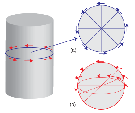
Figure 1: Cylindrical surface of a topological insulator nanowire and a typical spin configuration of a surface electronic state (left). Top view (a cross section is shown) of the spin configuration (right) in the (a) presence and (b) absence of cylindrical symmetry. In case (b) the spin follows the tangential plane of an auxiliary elliptic surface.

The appearance of spin Berry phase $\pi$ is a characteristic feature of topological insulator surface state, Xia et al. (2009) distinguishing it from, e.g., a carbon nanotube, Saito et al. (1992) another 2D gapless Dirac system (i.e., graphene) rolled up into a cylinder. These two Dirac systems both involve an effective spin degree of freedom appearing in the low-energy effective Hamiltonian. The physical origins of these spin degrees of freedom are different in the two cases; in the case of graphene (or carbon nanotube) it is the sub-lattice structure of hexagonal lattice, whereas in the present example it is essentially a genuine electron spin. These two effective spin degrees of freedom, despite their very different nature, play a similar role in determining the transport characteristics of the surface states on a flat surface. This is, however, no longer the case when the surface is curved. The sub-lattice pseudo-spin of graphene is insensitive to warping of the 2D plane. The effective spin on the surface of a topological insulator is, on the contrary, constrained to lie in-plane to the surface. Hsieh et al. (2009) This constraint is the origin of the spin Berry phase $\pi$ characteristic to the topological insulator surface state. Zhang et al. (2009); Zhang and Vishwanath (2010); Ostrovsky et al. (2010) One of the purposes of the present work is to demonstrate through explicit examples how the information encoded within the bulk Hamiltonian manifests itself in the surface effective Hamiltonian in the form of a nontrivial spin Berry phase. In the course of deriving the spin Berry phase, we also establish an unambiguous correspondence between the effective spin degree of freedom appearing in the 2D surface Dirac Hamiltonian and the original real spin embedded into the 3D bulk effective Hamiltonian.

A second motivation of this work is to explore the consequences of the anisotropy of topological insulators on the surface states, especially on the spin Berry phase. A rectangular nanowire made of such asymmetric compounds have surfaces of different symmetries. For example, in the Bi₂Se₃ nanowire studied in Ref. Peng et al. (2010) the surfaces orthogonal to the $c$-axis is rotationally symmetric, whereas surfaces parallel to the $c$-axis is not. Correspondingly, the surface Dirac cones are symmetric in the former, whereas distorted in the latter. The slope of the energy dispersion (Fermi velocity) also differs. What happens to the electron when it goes through (or gets reflected? by) junctions between two surfaces of different character? What is the fate of the Berry phase $\pi$ when an electron goes around the nanowire passing by several of such junctions? Such effects of anisotropy and multiple surface geometry will be also important in a similar Josephson-Majorana geometry involving metallic surface and Majorana bound states. Ioselevich and Feigel’man (2011)

This paper is organized as follows: we first demonstrate (Sec. II) by a simple analytic calculation that in the presence of anisotropy the surface effective spin is no longer strictly locked in-plane to the tangential plane on a curved surface, but it has generally a finite out-of-plane component.Kundu et al. (2011) We also show that only the global Berry phase $\pi$ which an electron acquires when it winds around a cylinder is robust against such asymmetry of the crystal. This point is further confirmed numerically by implementing a topological insulator nanowire penetrated by a $\pi$-flux tube as a tight-binding model on a square lattice (Sec. III).

II Derivation of the spin Berry phase

Let us first derive the spin Berry phase $\pi$ directly from a bulk 3D effective Hamiltonian. In contrast to Refs. Zhang et al. (2009); Zhang and Vishwanath (2010); Ostrovsky et al. (2010), here, we choose to go back to the 3D bulk effective Hamiltonian, and derive the spin Berry phase directly from the 3D Hamiltonian.

II.1 Cylindrical nanowire in parallel with the crystal growth axis

Let us start with the case in which the system has a cylindrical symmetry, i.e., a bulk insulating state is confined inside a cylinder of a radius $R$: $\sqrt{x^{2}+y^{2}}\leq R$, directed along a crystal growth axis ($c$-axis) perpendicular to the stacking layers. To describe the bulk insulating state, which is in contact with the vacuum outside the cylinder, we take the following effective Hamiltonian,Zhang et al. (2010); Liu et al. (2010); Shan et al. (2010)

$$H_{3D}=\left[\begin{array}[]{cccc}M&Bk_{z}&0&Ak_{-}\\ Bk_{z}&-M&Ak_{-}&0\\ 0&Ak_{+}&M&-Bk_{z}\\ Ak_{+}&0&-Bk_{z}&-M\end{array}\right].$$ (1)

This Hamiltonian describes a 3D Dirac system with a mass parameter $M=M_{0}+M_{2}(k_{x}^{2}+k_{y}^{2}+k_{z}^{2})$. The nature of the insulating state, i.e., whether it is $\mathbb{Z}_{2}$ trivial or not, is determined by the sign of $M_{0}/M_{2}$. When $M_{0}/M_{2}<0$, the insulating state is $\mathbb{Z}_{2}$ nontrivial: $\nu=1$ (the gap is inverted) exhibiting a single gapless surface Dirac cone, whereas when $M_{0}/M_{2}<0$, $\mathbb{Z}_{2}$ index is $\nu=0$ and the gap is normal. We regard here $A$ and $B$ to be constant; $A=A_{0}$, $B=B_{0}$ in the parametrization of Ref. Liu et al. (2010). Note that the same is assumed in the derivation of flat surface states in Ref. Liu et al. (2010). The anisotropy of the crystal is reflected in the asymmetry between $A$ and $B$; according to Table IV of Ref. Liu et al. (2010), $B_{0}$ is generally smaller then $A_{0}$, and in the case of Bi₂Te₃ smaller by one order of magnitude. The structure of the Hamiltonian (1) may become clearer in the follwoing symbolic form:

$$H=M\tau_{z}+Bk_{z}\tau_{x}\sigma_{z}+A\tau_{x}(k_{x}\sigma_{x}+k_{y}\sigma_{y}),$$ (2)

where $\bm{\tau}=(\tau_{x},\tau_{y},\tau_{z})$ and $\bm{\sigma}=(\sigma_{x},\sigma_{y},\sigma_{z})$ are two sets of Pauli matrices representing, respectively, an orbital and a spin degrees of freedom.

To identify the gapless surface states in the cylindrical geometry, we first decompose, in the spirit of Ref. Liu et al. (2010); Shan et al. (2010), the bulk 3D effective Hamiltonian (1) into two parts:

$$H=H_{\perp}(k_{r})+H_{\parallel}(k_{\phi},k_{z}),$$ (3)

where $H_{\perp}=H|_{k_{\phi}=k_{z}=0}$. $k_{r}$ and $k_{\phi}$ are components of the crystal momentum conjugate to the cylindrical coordinates:

$$r=\sqrt{x^{2}+y^{2}},\ \ \ \phi=\arctan{y\over x}.$$ (4)

$H_{\perp}$ is a Hamiltonian at the $\Gamma$-point, and reads explicitly,

$$H_{\perp} = M_{\perp}\tau_{z}+Ak_{r}\tau_{x}(\sigma_{x}\cos\phi+\sigma_{y}\sin\phi)$$ (5)

$$= \left[\begin{array}[]{cccc}M_{\perp}&0&0&Ae^{-i\phi}k_{r}\\ 0&-M_{\perp}&Ae^{-i\phi}k_{r}&0\\ 0&Ae^{i\phi}k_{r}&M_{\perp}&0\\ Ae^{i\phi}k_{r}&0&0&-M_{\perp}\end{array}\right].$$ (10)

For a later use, note also that the remaining $H_{\parallel}$ becomes

$$H_{\parallel}=\left[\begin{array}[]{cccc}M_{\parallel}&Bk_{z}&0&-iAe^{-i\phi}k_{\phi}\\ Bk_{z}&-M_{\parallel}&-iAe^{-i\phi}k_{\phi}&0\\ 0&iAe^{i\phi}k_{\phi}&M_{\parallel}&-Bk_{z}\\ iAe^{i\phi}k_{\phi}&0&-Bk_{z}&-M_{\parallel}\end{array}\right].$$ (11)

In Eqs. (10) and (11) we have decomposed the mass term into $M_{\perp}\simeq M_{0}+M_{2}k_{r}^{2}$ and $M_{\parallel}=M_{2}(k_{\phi}^{2}+k_{z}^{2})$. Of course, the Laplacian in the cylindrical coordinates has another contribution, $(1/r)\partial/\partial r$. Here, we neglect this first-order derivative term, keeping the term $\partial^{2}/\partial r^{2}$, which is a posteori justified, since the penetration depth $\lambda$ of the surface state is much smaller than the radius of the cylinder; $R\gg\lambda$.

We then consider a solution of the eigenvalue equation,

$$H_{\perp}|\psi\rangle=E_{\perp}|\psi\rangle$$ (12)

of the form, Zhou et al. (2008); Imura et al. (2010); Liu et al. (2010); Shan et al. (2010)

$$|\psi\rangle\sim e^{\lambda(r-R)},$$ (13)

i.e., $k_{r}=-i\lambda$ (we keep only $\lambda>0$). For a given $E_{\perp}$, one finds four independent solutions of this form, $|\psi\rangle=|\psi_{j}\rangle$ ($j=1,2,3,4$). Then one composes a linear combination of these four solutions,

$$|\psi\rangle=\sum_{j=1}^{4}c_{j}|\psi_{j}\rangle,$$ (14)

for satisfying the boundary condition:

$$|\psi\rangle_{r=R}=\left[\begin{array}[]{c}0\\ 0\\ 0\\ 0\end{array}\right].$$ (15)

The boundary condition (15) gives a restriction to the spinor part of the wave function $|\psi\rangle$, allowing for explicitly writing down its two independent bases.

To find the eigenspinors, which compose the spinor part of $|\psi_{j}\rangle$, one needs to diagonalize $H_{\perp}$. In view of its specific form written symbolically as in Eq. (5), one may diagonalize its real spin part first. Namely, one can partially diagonalize $H_{\perp}$ as,

$$H_{\perp}|\bm{r}\pm\rangle=\left(M_{\perp}\tau_{z}\pm Ak_{r}\tau_{x}\right)|\bm{r}\pm\rangle,$$ (16)

in terms of the following (real) spin eigenstates pointed in the radial direction $\hat{\bm{r}}=(\cos\phi,\sin\phi)$;

$$|\bm{r}+\rangle={1\over\sqrt{2}}\left[\begin{array}[]{c}1\\ e^{i\phi}\end{array}\right],\ \ |\bm{r}-\rangle={1\over\sqrt{2}}\left[\begin{array}[]{c}1\\ -e^{i\phi}\end{array}\right].$$ (17)

Here, we have chosen these eigenspinors single-valued. It is possible, of course, to take them double valued, but the two choices turn out to be completely equivalent. The advantage of the single-valued choice is that the Berry phase becomes explicit in the surface effective Hamiltonian; see Eq. (43). Whether one chooses one set of $|\bm{r}\pm\rangle$ or the other, they compose a set of bases diagonalizing real spin states pointed in the direction of $\hat{\bm{r}}$.

The remaining orbital ($\tau$-) part can be also diagonalized as,

$$H_{\perp}|\lambda\pm\rangle|\bm{r}\pm\rangle = E_{\perp}|\lambda\pm\rangle|\bm{r}\pm\rangle,$$

$$|\lambda\pm\rangle = \left[\begin{array}[]{c}1\\ \pm i(E_{\perp}-M_{\perp})/(\lambda A)\end{array}\right].$$ (20)

In the second line we took $k_{r}=-i\lambda$ explicitly into account. For a given energy $E_{\perp}$ satisfying $E_{\perp}^{2}=M_{0}-M_{2}\lambda^{2}$, there are four possible solutions for the penetration depth, $\lambda=\pm\lambda^{(\pm)}$, of which we keep only the two positive solutions, $\lambda=\lambda^{(\pm)}$. For each of $\lambda=\lambda^{(\pm)}$ we have two independent base spinors $|\lambda\pm\rangle$; we have in total four independent solutions, constituting the general solution (14). To be explicit, the general solution (14) reads explicitly,

$$|\psi\rangle=\left[c_{1}|\lambda^{(+)}+\rangle|\bm{r}+\rangle+c_{2}|\lambda^{(+)}-\rangle|\bm{r}-\rangle\right]e^{\lambda^{(+)}(r-R)}$$

$$+\left[c_{3}|\lambda^{(-)}+\rangle|\bm{r}+\rangle+c_{4}|\lambda^{(-)}-\rangle|\bm{r}-\rangle\right]e^{\lambda^{(-)}(r-R)}.$$ (21)

Notice that in Eq. (20) $E_{\perp}$ and $M_{\perp}$ are also functions of $\lambda$; $E_{\perp}=E_{\perp}(\lambda^{(\pm)})\equiv E_{\perp}^{(\pm)}$, $M_{\perp}=M_{\perp}(\lambda^{(\pm)})\equiv M_{\perp}^{(\pm)}$. The last step is to impose the boundary condition (15) to Eq. (II.1).

Since the two base spinors $|\bm{r}+\rangle$ and $|\bm{r}+\rangle$ subtend orthogonal real spin subspaces, the boundary condition (15) requires that

$$c_{1}|\lambda^{(+)}+\rangle+c_{3}|\lambda^{(-)}+\rangle = \left[\begin{array}[]{c}0\\ 0\end{array}\right],$$ (24)

$$c_{2}|\lambda^{(+)}-\rangle+c_{4}|\lambda^{(-)}-\rangle = \left[\begin{array}[]{c}0\\ 0\end{array}\right],$$ (27)

independently hold. This means that the spinor part of Eq. (II.1) can be expressed solely in terms of the eigen spinors, say, with $\lambda=\lambda^{(+)}$, i.e., as a linear combination of $|\lambda^{(+)}+\rangle$ and $|\lambda^{(+)}-\rangle$. The first line of Eq. (27) implies,

$$\det\left[\begin{array}[]{cc}-i\lambda^{(+)}A&-i\lambda^{(-)}A\\ E_{\perp}^{(+)}-M_{\perp}^{(+)}&E_{\perp}^{(-)}-M_{\perp}^{(-)}\end{array}\right]=0.$$ (28)

One can verify that this holds true only when the two conditions: (i) $M_{0}M_{2}<0$ (the system is in the $\nu=1$ phase) and (ii) $E_{\perp}=0$ are simultaneously satisfied. Substitute $E_{\perp}=0$ into Eq. (20), and notice that $M_{\perp}=-\lambda A$ is the only choice consistent with the requirement that $\lambda>0$, if one defines the parameters such that $A>0$ and $M_{2}>0$.

Taking all these into account one can express the solution of the boundary problem as,

$$|\psi\rangle = \left[c_{1}|\lambda^{(+)}+\rangle|\bm{r}+\rangle+c_{2}|\lambda^{(+)}-\rangle|\bm{r}-\rangle\right]\rho(r)$$ (29)

$$= \left[{c_{1}\over 2}\left[\begin{array}[]{c}1\\ i\\ e^{i\phi}\\ ie^{i\phi}\end{array}\right]+{c_{2}\over 2}\left[\begin{array}[]{c}1\\ -i\\ -e^{i\phi}\\ ie^{i\phi}\end{array}\right]\right]\rho(r)$$ (38)

$$\equiv c_{1}|\bm{r}+\rangle\rangle+c_{2}|\bm{r}-\rangle\rangle$$ (39)

where

$$\rho(r)\simeq{\sqrt{\lambda_{+}\lambda_{-}(\lambda_{+}+\lambda_{-})/\pi R}\over|\lambda_{+}-\lambda_{-}|}\left[e^{\lambda_{+}(r-R)}-e^{\lambda_{-}(r-R)}\right],$$ (40)

($\lambda_{\pm}\ll R$ assumed) and,

$$\lambda_{\pm}={A\pm\sqrt{A^{2}+4M_{0}M_{2}}\over 4M_{2}}.$$ (41)

The four-component eigenspinors $|\bm{r}\pm\rangle\rangle$ introduced in Eq. (39) describe electronic states localized in the vicinity of the surface. The effective 2D surface Hamiltonian $H_{2D}$ is obtained by calculating the matrix elements of $H_{\parallel}$ in terms of these $|\bm{r}\pm\rangle\rangle$, i.e.,

$$(H_{2D})_{\pm\pm}=\langle\langle\bm{r}\pm|H_{\parallel}|\bm{r}\pm\rangle\rangle.$$ (42)

By an explicit calculation, $H_{2D}$ is found to be

$$H_{2D}=$$ (43)

$$\left[\begin{array}[]{cc}0&-iBk_{z}+{A\over R}\left(-i{\partial\over\partial\phi}+{1\over 2}\right)\\ iBk_{z}+{A\over R}\left(-i{\partial\over\partial\phi}+{1\over 2}\right)&0\end{array}\right],$$ (46)

where we have used, $k_{\phi}\simeq-i(1/R)\partial/\partial\phi$, since $R\gg\lambda$, i.e., only $r\simeq R$ is relevant. Two factors $1/2$ which have appeared in the off-diagonal elements of Eq. (43) are the spin Berry phase terms, which lead to a $\pi$-phase shift when an electron goes around the cylinder. This Berry phase term can be eliminated from the eigenvalue equation for $H_{2D}$

$$H_{2D}\left[\begin{array}[]{c}c_{1}\\ c_{2}\end{array}\right]=E_{\parallel}\left[\begin{array}[]{c}c_{1}\\ c_{2}\end{array}\right]$$ (47)

by introducing a singular gauge transformation,

$$\bm{c}=\left[\begin{array}[]{c}c_{1}\\ c_{2}\end{array}\right]=e^{-i\phi/2}\left[\begin{array}[]{c}\chi_{1}\\ \chi_{2}\end{array}\right].$$ (48)

In the transformed $\chi$-basis, the surface Hamiltonian takes a simple Dirac form without the Berry phase,

$$H_{2D}^{(\bm{\chi})}=A\sigma_{x}k_{\phi}+B\sigma_{y}k_{z},$$ (49)

whereas the corresponding eigenspinors,

$$\bm{\chi}=\left[\begin{array}[]{c}\chi_{1}\\ \chi_{2}\end{array}\right],$$ (50)

become double-valued.

It is suggestive to express $\bm{\chi}$ explicitly in terms of a set of polar coordinates defined in the effective surface spin space. By introducnig the parameters as,

$$\cos\eta={Ak_{\phi}\over\sqrt{A^{2}k_{\phi}^{2}+Bk_{z}^{2}}},\ \ \sin\eta={Bk_{z}\over\sqrt{A^{2}k_{\phi}^{2}+Bk_{z}^{2}}},$$ (51)

the eigenstates of Eq. (49), corresponding to the eigenenergies,

$$E_{\parallel}=\pm\sqrt{A^{2}k_{\phi}^{2}+Bk_{z}^{2}},$$ (52)

can be written, respectively, as

$$\bm{\chi}={1\over\sqrt{2}}\left[\begin{array}[]{c}e^{-i\eta/2}\\ \pm e^{i\eta/2}\end{array}\right].$$ (53)

Comparing this with the textbook formula of an SU(2) spinor,

$$|\hat{\bm{n}}\pm\rangle=\left[\begin{array}[]{c}e^{-i\eta/2}\cos(\theta/2)\\ \pm e^{i\eta/2}\sin(\theta/2)\end{array}\right],$$ (54)

pointed in the direction of a unit vector $\hat{\bm{n}}$ specified by a polar angle $\theta$ and an azimuthal angle $\eta$ of the SU(2) spin space: $(s_{x},s_{y},s_{z})$, one can verify that the surface effective spin is locked in the $(s_{x},s_{y})$-plane, i.e., $\theta=\pi/2$.

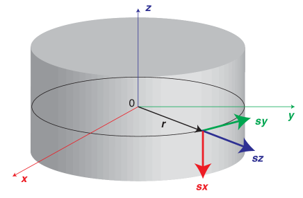
Figure 2: Spin coordinates on the cylindrical surface.

In the derivation of Eq. (43), we have chosen the spin quantization axis in the direction of $\hat{\bm{r}}$; see Eq. (17). Then, on which plane is the surface $(c_{1},c_{2})$-spin actually locked? In accordance with Eq. (17), the spin-space coordinates should be redefined as

$$\hat{\bm{s}}_{x}:\ \ \hat{\bm{x}} \rightarrow -\hat{\bm{z}},$$

$$\hat{\bm{s}}_{y}:\ \ \hat{\bm{y}} \rightarrow \hat{\bm{\phi}},$$

$$\hat{\bm{s}}_{z}:\ \ \hat{\bm{z}} \rightarrow \hat{\bm{r}},$$ (55)

on the cylindrical surface (see FIG. 2), since $k_{\phi}$ ($k_{z}$) play the role of $k_{y}$ ($-k_{x}$), where $\hat{\bm{\phi}}=(-\sin\phi,\cos\phi)$. Taking this into account, one can interpret Eq. (49), neglecting the anisotropy ($B=A$), as

$$H_{2D}^{(\bm{\chi})}\sim A(\bm{\sigma}\times\bm{k})_{z}.$$ (56)

In this regard, one can view Eq. (39) with coefficients $\chi_{1}$ and $\chi_{2}$ given in Eq. (53) as an SU(2) spin state,

$$|\bm{r}\pm\rangle=\chi_{1}|\bm{r}+\rangle+\chi_{2}|\bm{r}-\rangle,$$ (57)

decorated by an accompanying orbital degree of freedom. Eq. (57) represents a spin state which is locked in the plane perpendicular to $\hat{\bm{r}}$; unit normal vector of the cylindrical surface. This is a clear indication that the effective spin on the surface of a topological insulator cylinder is a real spin which is locked at each point of the cylinder in-plane to its tangential surface [FIG. 1, panel (a)], unlike the sub-lattice pseudo-spin on the cylindrical surface of a carbon nanotube. Saito et al. (1992)

One step backward, notice that this peculiar property of the spin Berry phase $\pi$ manifest in Eqs. (43) and (48) is here not derived from the property of the effective Dirac Hamiltonian, i.e., Eq. (49) on the cylindrical coordinates. It was encoded in the dependence of eigenspinors (29) on the spatial angle $\phi$, and the explicit form of $H_{\parallel}$ as given in Eq. (11). In Refs. Zhang et al. (2009); Zhang and Vishwanath (2010); Ostrovsky et al. (2010) the same conclusion was drawn by observing the surface effective Hamiltonian on a curved surface. Here, the Dirac equation was derived simultaneously with the spin Berry phase; the existence of the spin Berry phase is indeed encoded in the bulk 3D Hamiltonian.

II.2 Cylindrical nanowire perpendicular to the crystal growth axis

We have considered so far electronic states on the surface of a cylinder whose axis of symmetry is pointed along the $c$-axis, i.e., in the direction of crystal anisotropy. Since the rotational symmetry around the $c$-axis is presumed, any tangential surface of the cylinder is equivalent. Under such circumstances, we have seen explicitly that the effective spin degree of freedom appearing in the Dirac equation (43) is constrained to the curved (cylindrical) surface.

Here, we consider a less trivial case of broken rotational symmetry, i.e., with the cylindrical axis chosen perpendicular to the $c$-axis. Of course, nanowires are not cylindrical in real samples, but have several surfaces. It is also unlikely that the axis of the wire is perfectly aligned with the axis of crystal symmetry ($c$-axis). In the presence of such rotational anisotropy, it is less trivial whether the effective spin degree of freedom on the surface is always tied to the curved surface.

To implement an anisotropic cylindrical surface we consider here the case of the crystal $c$-axis pointed in the $x$-direction, keeping the symmetry axis of the cylinder pointed always in the $z$-direction; obviously, one can equally rotate the cylinder in the $y$-direction with keeping the crystal growth axis in the $z$-direction. The bulk effective Hamiltonian as Eq. (2) for such a rotated crystal becomes (here, we do rotate the crystal),

$$H_{3D}=M\tau_{z}+\tau_{x}(B\sigma_{x}k_{x}+A\sigma_{y}k_{y}+A\sigma_{z}k_{z}).$$ (58)

To identify the surface electronic states which span the basis for the 2D surface Dirac Hamiltonian, we introduce the same cylindrical coordinate as Eq. (4) and decompose the Hamiltonian (58) into perpendicular ($H_{\perp}$) and parallel ($H_{\parallel}$) components in parallel with Eqs. (3), (10) and (11). Some parameters need, of course, redefinition or exchange. Let us first focus on

$$H_{\perp}=M_{\perp}\tau_{z}+k_{r}\tau_{x}(B\sigma_{x}\cos\phi+A\sigma_{y}\sin\phi).$$ (59)

To diagonalize the real spin part of the Hamiltonian (59), it is convenient to introduce an auxiliary angle $\tilde{\phi}$, defined as,

$$B\cos\phi=\tilde{A}\cos\tilde{\phi},$$

$$A\sin\phi=\tilde{A}\sin\tilde{\phi},$$ (60)

where

$$\tilde{A}=\tilde{A}(\phi)=\sqrt{B^{2}\cos^{2}\phi+A^{2}\sin^{2}\phi}.$$ (61)

In analogy with Eq. (16), one can partially diagonalize Eq. (59) as

$$H_{\perp}|\tilde{\bm{r}}\pm\rangle=\left(M_{\perp}\tau_{z}\pm\tilde{A}k_{r}\tau_{x}\right)|\tilde{\bm{r}}\pm\rangle,$$ (62)

but here the eigenspinors represent no longer spin states in the $\hat{\bm{r}}$-direction normal to the surface of the cylinder. The new eigenspinors $|\tilde{\bm{r}}\pm\rangle$ are formally analogous to $|\bm{r}\pm\rangle$ defined as in Eqs. (17), but pointed in the direction specified by $\tilde{\phi}$ introduced above;

$$|\tilde{\bm{r}}+\rangle={1\over\sqrt{2}}\left[\begin{array}[]{c}1\\ e^{i\tilde{\phi}}\end{array}\right],\ \ |\tilde{\bm{r}}-\rangle={1\over\sqrt{2}}\left[\begin{array}[]{c}1\\ -e^{i\tilde{\phi}}\end{array}\right].$$ (63)

The remaining procedure is perfectly in parallel with the previous case. After imposing the boundary condition on the cylindrical surface of the topological insulator, one finds as the basis spinors for constructing the surface effective Hamiltonian,

$$|\psi\rangle = \left[c_{1}|\lambda^{(+)}+\rangle|\tilde{\bm{r}}+\rangle+c_{2}|\lambda^{(+)}-\rangle|\tilde{\bm{r}}-\rangle\right]\rho(r)$$ (64)

$$= \left[{c_{1}\over 2}\left[\begin{array}[]{c}1\\ i\\ e^{i\tilde{\phi}}\\ ie^{i\tilde{\phi}}\end{array}\right]+{c_{2}\over 2}\left[\begin{array}[]{c}1\\ -i\\ -e^{i\tilde{\phi}}\\ ie^{i\tilde{\phi}}\end{array}\right]\right]\rho(r)$$ (73)

$$\equiv c_{1}|\tilde{\bm{r}}+\rangle\rangle+c_{2}|\tilde{\bm{r}}-\rangle\rangle,$$ (74)

where $\rho(r)$ is given as in Eq. (40) with a normalization factor expressed in terms of $\lambda_{\pm}$ given as in Eq. (41) but with $A$ replaced by $\tilde{A}$ given in Eq. (61).

To find the surface effective Hamiltonian, we calculate again the matrix elements of $H_{\parallel}$, here, in terms of $|\tilde{\bm{r}}\pm\rangle\rangle$ associated with $|\tilde{\bm{r}}\pm\rangle$ introduced in Eqs. (63). We have introduced the parameter $\tilde{\phi}$ in Eqs. (II.2) and was able to construct the basis spinors $|\tilde{\bm{r}}\pm\rangle\rangle$ which successfully span the subspace representing the solution of the boundary problem. $\tilde{\phi}$-parametrization was useful, since $H_{\perp}$ shows a nice transformation property in terms of $\tilde{\phi}$. It is, however, no longer the case for $H_{\parallel}$, which reads explicitly in the present case,

$$H_{\parallel} = M_{\parallel}\tau_{z}+A\tau_{x}\sigma_{z}k_{z}$$ (75)

$$+ \tau_{x}(-B\sigma_{x}\sin\phi+A\sigma_{y}\cos\phi)k_{\phi}$$

$$= \left[\begin{array}[]{cccc}M_{\parallel}&Ak_{z}&0&-ic_{\phi}k_{\phi}\\ Ak_{z}&-M_{\parallel}&-ic_{\phi}k_{\phi}&0\\ 0&ic_{\phi}^{*}k_{\phi}&M_{\parallel}&-Ak_{z}\\ ic_{\phi}^{*}k_{\phi}&0&-Ak_{z}&-M_{\parallel}\end{array}\right],$$ (80)

where we have introduced

$$c_{\phi}=A\cos\phi-iB\sin\phi.$$ (81)

$c_{\phi}$ is a complex number which is a function of the real parameter $\phi$. Note that $c_{\phi}$ does not simplify with the use of $\tilde{\phi}$.

To derive the surface effective Hamiltonian $H_{2D}$, one calculates again the matrix elements, $\langle\langle\tilde{\bm{r}}\pm|H_{\parallel}|\tilde{\bm{r}}\pm\rangle\rangle$ in terms of the new $\tilde{\bm{r}}$-basis. One can explicitly verify that diagonal elements of the surface effective Hamiltonian vanish, i.e.,

$$\tilde{H}_{2D}=\left[\begin{array}[]{cc}0&\langle\langle\tilde{\bm{r}}+|H_{\parallel}|\tilde{\bm{r}}-\rangle\rangle\\ \langle\langle\tilde{\bm{r}}-|H_{\parallel}|\tilde{\bm{r}}+\rangle\rangle&0\end{array}\right].$$ (82)

The off-diagonal elements involve a first-order derivative with respect to $\phi$, yielding a Berry phase term; e.g.,

$$\langle\langle\tilde{\bm{r}}+|H_{\parallel}|\tilde{\bm{r}}-\rangle\rangle=$$

$$-iAk_{z}+{1\over 2}\left(c_{\phi}k_{\phi}e^{i\tilde{\phi}}+e^{-i\tilde{\phi}}c_{\phi}^{*}k_{\phi}\right).$$ (83)

Note that terms coming from the $\phi$-dependence of $\lambda_{\pm}$, given as in Eq. (41), cancel when integrated over $r$. The $\phi$-dependence exists not only in the explicit $r$-dependence of $\rho(r)$ on $\lambda_{\pm}$; cf. Eq. (40), but also in the normalization factor of $\rho(r)$. The $\phi$-dependence of $\lambda_{\pm}$ stems from that of $\tilde{A}=\tilde{A}(\phi)$. In Eq. (83) the Berry phase term appears in the second part when $k_{\phi}$ acts on the exponent of $e^{i\tilde{\phi}}$, and is found to be of the form,

$$\Omega(\phi)={c_{\phi}e^{i\tilde{\phi}}\over 2R}{d\tilde{\phi}\over d\phi}={c_{\phi}e^{i\tilde{\phi}}\over 2R}{AB\over\tilde{A}^{2}}.$$ (84)

Notice that only the real part of this factor influences the phase of the wave function and is identified as the local spin Berry phase. This phase factor can be eliminated from the eigenvalue equation: $\tilde{H}_{2D}\bm{c}=E_{\parallel}\bm{c}$, by employing a singular gauge transformation analogous to Eq. (48), i.e., by $\bm{c}=e^{-i\tilde{\phi}/2}\bm{\chi}$. Since $\phi$ and $\tilde{\phi}$ have the same winding property,

$$\tilde{\phi}(\phi+2\pi)-\tilde{\phi}(\phi)=2\pi,$$ (85)

the eigenspinor, Eq. (50) is precisely double-valued with respect to a $2\pi$-rotation of $\phi$, i.e., the spin Berry phase is just $\pi$.

The off-diagonal elements of Eq. (82) are also susceptible of the imaginary part of $\Omega(\phi)$ given as in Eq. (84). This imaginary part introduces a non-uniform modulation into the amplitude of the wave function of surface electronic states. Such a situation is somewhat similar to the case of a WKB wave function describing the system with a spatial non-uniformity. The phase of such WKB wave function is expressed in terms of a “wave vector” $k$ which depends on the space coordinate. Meanwhile its amplitude shows also a space dependence. In the present formulation, this appears as an imaginary part of $\Omega(\phi)$.

Let us come back to the question, “In which direction is the eigenspinor $\bm{c}$, or equivalently $\bm{\chi}$, pointed in the spin space?” Taking it into account that our surface effective Hamiltonian is defined on a space spanned by $|\tilde{\bm{r}}\pm\rangle\rangle$, we redefine the spin coordinates as,

$$\hat{\bm{s}}_{x}:\ \ \hat{\bm{x}} \rightarrow -\hat{\bm{z}},$$

$$\hat{\bm{s}}_{y}:\ \ \hat{\bm{y}} \rightarrow \tilde{\bm{\phi}},$$

$$\hat{\bm{s}}_{z}:\ \ \hat{\bm{z}} \rightarrow \tilde{\bm{r}},$$ (86)

where $\tilde{\bm{\phi}}=(-\sin\tilde{\phi},\cos\tilde{\phi})$. This means that the eigenstate $\bm{c}$ of $\tilde{H}_{2D}$ given in Eq. (82) can be viewed as an SU(2) spin state,

$$|\tilde{\bm{r}}\pm\rangle=b_{1}|\tilde{\bm{r}}+\rangle+b_{2}|\tilde{\bm{r}}-\rangle,$$ (87)

accompanied by orbital spins. Eq. (87) represents a spin state locked in the plane perpendicular to $\tilde{\bm{r}}$. Note that $\tilde{\bm{r}}$ is not a unit vector normal to the cylinder surface. Thus in the case of broken cylindrical symmetry, the surface effective spin can have a finite component normal to a tangential surface of the cylinder [FIG. 1, panel (b)]. An out-of-plane component of the surface effective spin appears also as a consequence of the hexagonal warping, Fu (2009); Xu et al. (2011); Souma et al. (2011) and in a system of topological insulator quantum dot. Kundu et al. (2011)

In this section, we have examined the electronic states on cylindrical surfaces of an anisotropic topological insulator. An explicit one-to-one correspondence between the effective spin in the surface Dirac Hamiltonian and the real spin inherent to the 3D bulk effective Hamiltonian has been established. The existence of spin Berry phase $\pi$ has been unambiguously shown in this context. In the cylindrically symmetric case (Sec. II A), i.e., in the case of a cylindrical nanowire parallel to the crystal $c$-axis, we have shown explicitly that the effective surface spin is constrained in-plane to the real-space tangential plane of the cylinder. In the absence of such cylindrical symmetry (Sec. II B: case of a cylindrical nanowire perpendicular to the crystal $c$-axis) the effective surface spin can have a finite amplitude in the direction normal to the cylindrical surface. However, when the reference point on the cylindrical surface travels once around the cylinder (i.e., winds the cylinder once), the resulting spin Berry phase is indeed $\pi$. This point will be further confirmed in the numerical experiments in Sec. III.

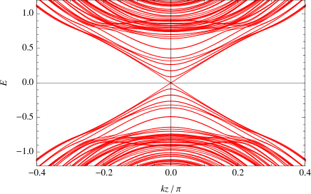
Figure 3: Energy spectrum $E(k_{z})$ of a topological insulator nanowire with a rectangular cross section ($N_{x}=12$, $N_{y}=16$). The horizontal axis $k_{z}$ represents the crystal momentum along the wire. The crystal anisotropy is introduced in the direction perpendicular to the wire (in the $x$-direction, $B/A=0.7$). $M_{0}/M_{2}=-1$ (STI with a surface Dirac cone at the $\Gamma$-point). The lower panel is for the same nanowire pierced by a $\pi$-flux tube. To avoid formation of a bound state, the $\pi$-flux is divided into two $\pi/2$-flux tubes penetrating two neighboring plaquettes in the wire center region.

III Energy spectrum in the presence of a $\pi$-flux tube

The spin Berry phase appearing in the surface Dirac Hamiltonian; cf. Eq. (43), is often discussed Zhang et al. (2009); Zhang and Vishwanath (2010); Ostrovsky et al. (2010); Bardarson et al. (2010); Rosenberg et al. (2010); Imura et al. (2011) in the context of Aharonov-Bohm experiment on topological insulator nanowires. Peng et al. (2010) Let us first recall that the existence of a spin Berry phase $\pi$ leads, on the surface of a cylindrical nanowire, to the appearance of a finite-size energy gap in the spectrum of surface electronic states. The spin Berry phase $\pi$ modifies the periodic boundary condition around the wire to an anti-periodic boundary condition, leading to opening of the gap. Let us explicitly see this. The wave function of such a surface electronic state is an eigenstate of Eq. (43), which is a plane wave,

$$\psi(z,\phi)=e^{ik_{z}z}e^{ik_{\phi}R\phi}.$$ (88)

The corresponding eigenenergy reads

$$E(k_{z},k_{\phi})=\pm A\sqrt{k_{z}^{2}+k_{\phi}^{2}}.$$ (89)

Here, we neglect the anisotropy ($B=A$). The energy spectrum $E(k_{z})$ of the surface electronic states is determined by imposing (anti-)periodic boundary condition to Eq. (88). The spin Berry phase $\pi$ replaces the periodic boundary condition:

$$\psi(z,\phi+2\pi)=\psi(z,\phi),$$ (90)

by an anti-periodic boundary condition,

$$\psi(z,\phi+2\pi)=-\psi(z,\phi),$$ (91)

shifting the allowed values of $k_{\phi}R$ from integers ($k_{\phi}R=0,\pm 1,\pm 2,\cdots$) to half odd integers ($k_{\phi}R=\pm 1/2,\pm 3/2,\cdots$). Importantly, the $k_{\phi}=0$ and correspondingly the zero-energy bound state was purged from the lowest energy portion of the spectrum by this $\pi$-phase shifting (cf. FIG. 3, upper panel). In the Aharonov-Bohm geometry, this finite-size energy gap associated with the spin Berry phase is compensated by an Aharonov-Bohm phase $\phi_{AB}$, and in some cases we expect the energy spectrum closes its gap.

In the previous section the spin Berry phase $\pi$ for surface electrons is derived in the presence and absence (due to crystal anisotropy) of cylindrical symmetry, that is, regardless of fulfilling the spin-to-surface locking condition. Here, we confirm numerically the robustness of the $\pi$ spin Berry phase against cylindrical symmetry breaking, using a tight-binding model for a topological insulator nanowire. We attempt to show that the amount of the ”integrated” Berry phase, corresponding to a $2\pi$-rotation of the azimuthal angle $\phi$, is precisely $\pi$. To verify this explicitly, we introduce a $\pi$ magnetic flux tube piercing the nanowire, as a probe, and investigate the corresponding energy spectrum. Exact cancellation of the spin Berry phase and the Aharonov-Bohm phase is confirmed by observing the closing of finite-size energy gap.

To implement a ”shape” in real space such as a nanowire we consider in the following a tight-binding version of Eq. (58) on a cubic lattice. We first make the following replacement:

$$k_{j}\rightarrow\sin k_{j},$$ (92)

where $j=x,y,z$, for the $k_{j}$’s in Eq. (58), and similarly,

$$k_{j}^{2}\rightarrow 2(1-\cos k_{j}),$$ (93)

for $k_{j}^{2}$’s in $M$. After this replacement the Hamiltonian (58) can be interpreted as a tight-binding Hamiltonian, i.e.,

$$H_{3D} = \sum_{x,y,z}\big{\{}(M_{0}+6M_{2})|x,y,z\rangle\langle x,y,z|$$ (94)

$$+ \big{(}t_{x}|x+1,y,z\rangle\langle x,y,z|+t_{y}|x,y+1,z\rangle\langle x,y,z|$$

$$+ t_{z}|x,y,z+1\rangle\langle x,y,z|+h.c.\big{)}\big{\}},$$

where

$$t_{x} = i{B\over 2}\tau_{x}\sigma_{x}-M_{2}\tau_{z},\ \ t_{y}=i{A\over 2}\tau_{x}\sigma_{y}-M_{2}\tau_{z}.$$

$$t_{z} = i{A\over 2}\tau_{x}\sigma_{z}-M_{2}\tau_{z}.$$ (95)

Depending on the value of $M_{0}/M_{2}$, the tight-binding Hamiltonian (94) describes either strong/weak topological insulators (STI/WTI) or an ordinary insulator; $-4<M_{0}/M_{2}<0$ and $-12<M_{0}/M_{2}<-8$ $\rightarrow$ STI, $-8<M_{0}/M_{2}<-4$ $\rightarrow$ WTI, $M_{0}/M_{2}<-12$ and $0<M_{0}/M_{2}$ $\rightarrow$ ordinary insulator. In the following, we will mainly focus on the case $-4<M_{0}/M_{2}<0$, corresponding to STI with a surface Dirac cone at the $\Gamma$-point. So far the Hamiltonian is translationally symmetric. We now restrict the electrons to move only inside the nanowire with a rectangular cross section: $1\leq x\leq N_{x}$, $1\leq y\leq N_{y}$. This can be done simply by switching off unnecessary hopping amplitudes. After this only $k_{z}$ remains to be a good quantum number; we always assume a periodic boundary condition in the $z$-direction.

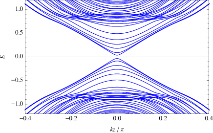
Figure 4: Energy spectrum $E(k_{z})$ and a typical shape of the (squared amplitude of) the lowest energy wave function in the presence of a $\pi$-flux tube penetrating a series of single plaquettes along the axis of nanowire. The cross section is rectangular, $N_{x}=12$, $N_{y}=16$, the anisotropy is $B/A=0.7$. $M_{0}/M_{2}=-1$. $M_{2}=A=1$. The wave function is depicted at $k_{z}/\pi=0.03$.

We then introduce an Aharonov-Bohm flux $\phi_{AB}$ piercing the nanowire. We consider typically the case of $\phi_{AB}=\pi$ (case of a $\pi$-flux tube). The simplest way to do this is to let a $\pi$-flux tube penetrate a central plaquette of each $z$-layer, e.g., the plaquette centered at $(x,y)=(N_{x}/2+1/2,N_{y}/2+1/2)$ for $N_{x}$ and $N_{y}$ being an even integer. The insertion of a flux can be achieved by Peierls substitution, e.g., $t_{x}\rightarrow t_{x}e^{i\phi_{AB}}$ for $x=N_{x}/2\rightarrow N_{x}/2+1$, $y=1,\cdots,N_{y}/2$. This turns out, however, to be not the best solution for us, since a $\pi$-flux tube penetrating a single plaquette involves a (zero-energy) bound state. Rosenberg et al. (2010); Juricic et al. (2011) In the nanowire geometry such a bound state appears as the lowest energy helical modes bound to the flux tube, propagating in the direction opposite to the preformed surface electronic states, i.e., electrons localized on the surface of the cylinder. Formation of such a pair of counter-propagating modes separated only by a finite distance leads naturally to gap opening (FIG. 4, upper panel); mixing of the two counter-propagating modes (see the wave function, in FIG. 4, lower panel) causes level repulsion between the two initially gapless states.

To avoid formation of such a bound state we rather introduce here a total magnetic flux $\pi$ divided into two $\pi/2$-flux tubes penetrating the two neighboring plaquettes, e.g., plaquettes centered at $(x,y)=(N_{x}/2-1/2,N_{y}/2+1/2)$ and $(N_{x}/2+1/2,N_{y}/2+1/2)$. With this we could see a clear signature of the finite-size gap closing (FIG. 3, lower panel). There appears no low-energy bound states around a $\pi/2$-flux tube. In the same figure one can actually recognize such bound states pushed up into the high-energy spectrum.

In the above example, by changing the amount of Aharonov-Bohm flux $\phi_{AB}=\pi,2\pi,3\pi,\cdots$, we find an even/odd feature (gapped, gapless, gapped, gapless, $\cdots$) in the energy spectrum of surface electronic states. An alternative way to verify explicitly that the amount of this Berry phase is precisely $\pi$ is to investigate a similar even/odd feature due to crystal dislocation lines (results not shown here). We have shown previously that the electronic states along such a dislocation or equivalently a nanowire exhibits a finite size energy gap, manifesting the existence of spin Berry phase. Imura et al. (2011)

What have we verified in these numerical simulations? (Especially in its relation to what we have discussed in Sec. II B.) In the example we have presented in this section the cylinder itself is distorted, having a rectangular cross section. In addition to such a structural asymmetry, we have also taken into account the crystal anisotropy. Our data indicate that the global spin Berry phase $\pi$ is robust under the coexistence of a structural asymmetry and a crystal anisotropy.

IV Conclusions

We have studied the electronic states on cylindrical surfaces of an anisotropic topological insulator. We have established an explicit one-to-one correspondence between the effective spin in the surface Dirac Hamiltonian and the real spin inherent to the 3D bulk effective Hamiltonian. The effective spin on the surface of a topological insulator has a property of being constrained on its tangential surface, and in particular, when its surface is warped (e.g., into a cylinder) the effective spin feels this change of tangential plane in real space, and consequently, the effective spin completes a $2\pi$ rotation when the reference point travels once around the cylinder. The existence of spin Berry phase $\pi$ is naturally understood in this context. However, on the surface of a topological insulator with broken cylindrical symmetry in the presence of crystal anisotropy, the effective spin does not follow locally the tangential plane in real space, i.e., the effective spin can have generally a component normal to the surface. This has been shown analytically in Sec. II B, using a rather simple model, Whereas, globally the spin Berry phase $\pi$ is robust against anisotropy and breaking of the cylindrical symmetry. The latter has been verified numerically in Sec. III.

In the examples we have considered in this paper, the “curved” surfaces did not really have a curvature; a cylindrical surface is flat in the proper use of terminology in differential geometry (its Riemann curvature is null). On a genuinely curved surface with a finite Riemann curvature, e.g., on a sphere, the concept of $\pi$ spin Berry phase may need some modification or a generalization. Naively, it is expected to involve a solid angle associated with parallel transport on a sphere. We leave future studies a more rigorous discussion on such an issue.