Neural networks with non-smooth and impact activations

Abstract

In this paper, we consider a model of impulsive recurrent neural networks with piecewise constant delay. The dynamics are presented by differential equations with discontinuities such as impulses at fixed moments and piecewise constant argument of generalized type. Sufficient conditions ensuring the existence, uniqueness and global asymptotic stability of the equilibrium point are obtained. By employing Green’s function we derive new result of existence of the periodic solution. The global asymptotic stability of the solution is investigated. Examples with numerical simulations are given to validate the theoretical results.

and

1 Introduction

Recurrent neural networks and impulsive recurrent neural networks have been investigated due to their extensive applications in classification of patterns, associative memories, image processing, optimization problems, and other areas [17, 20, 21, 22, 23, 24, 25, 26, 27, 28, 29, 30, 31, 32]. It is well known that these applications depend crucially on the dynamical behavior of the networks. For example, if a neural network is employed to solve some optimization problems, it is highly desirable for the neural network to have a unique globally stable equilibrium [41, 42, 43, 44, 45, 46, 47, 48]. Therefore, stability analysis of neural networks has received much attention and various stability conditions have been obtained over the past years. Another interesting subject is to study the dynamical behavior of existence of the periodic solutions in recurrent neural networks. These periodic solutions present periodic pattern and have been used in learning theory, which are meant to capture the idea that certain activities or motions are learned by repetition [15, 16].

In numerical simulations and practical implementations of neural networks, it is essential to formulate a discrete-time system, an analogue of the continuous-time system. Hence, stability for discrete-time neural networks has also received considerable attention from many researchers [35, 36, 37, 38, 39, 40]. As we know, the reduction of differential equations with piecewise constant argument to discrete equations has been the main and possibly a unique way of stability analysis for these equations [49, 50]. Hence, one has not investigated the problem of stability completely, as only elements of a countable set were allowed to be discussed for initial moments. Finally, only equations which are linear with respect to the values of solutions at non-deviated moments of time have been investigated. That narrowed significantly the class of systems. In papers [3, 4, 5, 6], the theory of differential equations with piecewise constant argument has been generalized by Akhmet. Later, Akhmet gathered all results for this type of differential equations in the book [2]. All of these equations are reduced to equivalent integral equations such that one can investigate many problems, which have not been solved properly by using discrete equations, i.e., existence and uniqueness of solutions, stability and existence of periodic solutions. Moreover, since we do not need additional assumptions on the reduced discrete equations, the new method requires more easily verifiable conditions, similar to those for ordinary differential equations.

In this paper, we develop the model of recurrent neural networks to differential equations with both impulses and piecewise constant argument of generalized type. It is well known that impulsive differential equation [1, 11, 12] is one of the basic instruments so the role of discontinuity has been understood better for the real world problems. In real world, many evolutionary processes are characterized by abrupt changes at certain time. These changes are called to be impulsive phenomena, which are included in many fields such as biology involving thresholds, bursting rhythm models, physics, chemistry, population dynamics, models in economics, optimal control, etc. In the literature, recurrent neural networks have been developed by implementing impulses and piecewise constant delay [8, 9, 26, 27, 28, 29, 30, 31, 32] issuing from different reasons: In implementation of electronic networks, the state of the networks is subject to instantaneous perturbations and experiences abrupt change at certain instants which may be caused by switching phenomenon, frequency change or other sudden noise. Furthermore, the dynamics of quasi-active dendrites with active spines is described by a system of point hot-spots (with an integrate-and-fire process), see [33, 34] for more details. This leads to the model of recurrent neural network with impulses. It is important to say that the neighbor moments of impulses may depend on each other. For example, the successive impulse moment may depend upon its predecessor. The reason for this phenomenon is the interior design of a neural network. On the other hand, due to the finite switching speed of amplifiers and transmission of signals in electronic networks or finite speed for signal propagation in neural networks, time delays exist [21, 22, 24, 25]. Moreover, the idea of involving delayed arguments in the recurrent neural networks can be explained by the fact that we assume neural networks may “memorize” values of the phase variable at certain moments of time to utilize the values during middle process till the next moment. Thus, we arrive to differential equations with piecewise constant delay. Obviously, the distances between the “memorized” moments may be very variative. Consequently, the concept of generalized type of piecewise constant argument is fruitful for recurrent neural networks [7, 8, 9]. Therefore, it is possible to apply differential equations with both impulses and piecewise constant delay to neural networks theory.

The intrinsic idea of the paper is that our model is not only from the applications point of view, but also from a new system of differential equations. That is, we develop differential equations with piecewise constant argument of generalized type to a new class of systems; impulsive differential equations with piecewise constant delay and apply them to recurrent neural networks [3, 4, 5, 6, 8, 9]. Another novelty of this paper is that the sequence of moments $\theta_{k},\ k\in\mathbb{N},$ where the constancy of the argument changes, and the sequence of impulsive moments, $\tau_{k},$ are different. More precisely, each moment $\tau_{i},\ i\in\mathbb{N},$ is an interior point of an interval $(\theta_{k},\theta_{k+1}).$ This gives to our investigations more biological sense, as well as provides new theoretical opportunities.

2 Model description and preliminaries

Let $\mathbb{N}=\{0,1,2,\ldots\}$ and $\mathbb{R}^{+}=[0,\infty)$ be the sets of natural and nonnegative real numbers, respectively, and denote a norm on $\mathbb{R}^{m}$ by $||\cdot||$ where $||u||=\displaystyle\sum^{m}_{i=1}|u_{i}|.$ Fix two real valued sequences $\theta=\left\{\theta_{k}\right\},\tau=\left\{\tau_{k}\right\},\ k\in\mathbb{N},\ \tau\cap\theta=\phi$ such that $\theta_{k}<\theta_{k+1}$ with $\theta_{k}\rightarrow\infty$ as $k\rightarrow\infty$ and $\tau_{k}<\tau_{k+1}$ with $\tau_{k}\rightarrow\infty$ as $k\rightarrow\infty,$ and there exist two positive numbers $\overline{\theta},\underline{\tau}$ such that $\theta_{k+1}-\theta_{k}\leq\overline{\theta}$ and $\underline{\tau}\leq\tau_{k+1}-\tau_{k},\ k\in{\mathbb{N}}.$ The condition of the empty intersection is caused by the investigation reasons. Otherwise, the proof of auxiliary results needs several additional assumptions.

The main subject under investigation in this paper is the following impulsive recurrent neural networks with piecewise constant delay

$$x^{\prime}_{i}(t) = -a_{i}x_{i}(t)+\displaystyle\sum_{j=1}^{m}b_{ij}f_{j}(x_{j}(t))$$

$$+\sum_{j=1}^{m}c_{ij}g_{j}(x_{j}(\beta(t)))+d_{i},\ t\not=\tau_{k}$$

$$\Delta x_{i}\mid_{t=\tau_{k}} = I_{ik}(x_{i}(\tau_{k}^{-})),\quad a_{i}>0,\ i=1,2,\cdots,m,\quad k\in\mathbb{N},$$ (2.1b)

where $\beta(t)=\theta_{k}$ (see Fig. 1) if $\theta_{k}\leq t<\theta_{k+1},\,k\in{\mathbb{N}},\,t\in{\mathbb{R}^{+}},$ is an identification function, $\Delta x_{i}(\tau_{k})$ denotes $x_{i}(\tau_{k})-x_{i}(\tau_{k}^{-}),$ where $x_{i}(\tau_{k}^{-})=\lim_{h\rightarrow 0^{-}}x_{i}(\tau_{k}+h).$ Moreover, $m$ corresponds to the number of units in a neural network, $x_{i}(t)$ stands for the state vector of the $i$th unit at time $t,$ $f_{j}(x_{j}(t))$ and $g_{j}(x_{j}(\beta(t)))$ denote, respectively, the measures of activation to its incoming potentials of the unit $j$ at time $t$ and $\beta(t),$ $b_{ij},c_{ij},d_{i}$ are real constants, $b_{ij}$ means the strength of the $j$th unit on the $i$th unit at time $t,$ $c_{ij}$ infers the strength of the $j$th unit on the $i$th unit at time $\beta(t),$ $d_{i}$ signifies the external bias on the $i$th unit and $a_{i}$ represents the rate with which the $i$th unit will reset its potential to the resting state in isolation when it is disconnected from the network and external inputs.

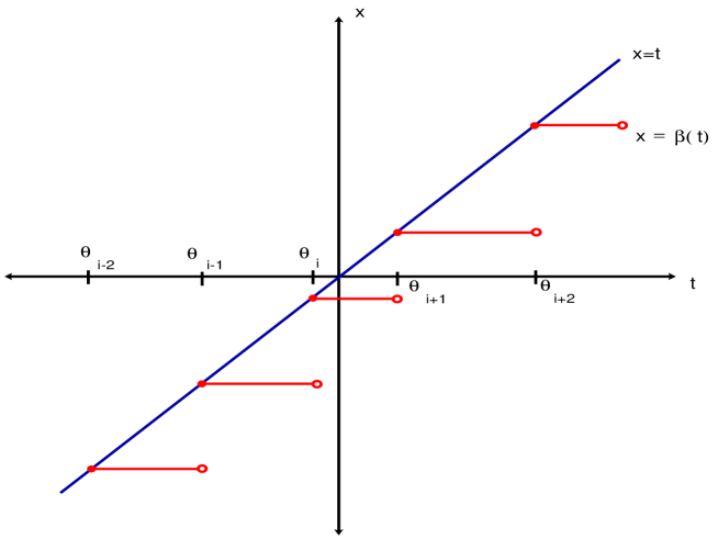
Figure 1: The graph of the argument $\beta(t).$

In the theory of differential equations with piecewise constant argument [3, 4, 5], we take the function $\beta(t)=\theta_{k}$ if $\theta_{k}\leq t<\theta_{k+1}$, that is, $\beta(t)$ is right continuous. However, as it is usually done in the theory of impulsive differential equations, at the points of discontinuity $\tau_{k}$ of the solution, solutions are left continuous. Thus, the right continuity is more convenient assumption if one considers equations with piecewise constant arguments, and we shall assume the continuity for both, impulsive moments and moments of the switching of constancy of the argument.

We say that the function $\varphi:\mathbb{R}^{+}\rightarrow\mathbb{R}^{m}$ is from the set $PC_{\tau}(\mathbb{R}^{+},{\mathbb{R}^{m}})$ if:

1. $\varphi$ is right continuous on $\mathbb{R}^{+};$

2. it is continuous everywhere except possibly moments $\tau$ where it has discontinuities of the first kind.

Moreover, we introduce a set of functions $PC_{\tau\cup\theta}(\mathbb{R}^{+},{\mathbb{R}^{m}})$ if we replace $\tau$ by $\tau\cup\theta$ in the last definition. In our paper, we understand that $\varphi:\mathbb{R}^{+}\rightarrow\mathbb{R}^{m}$ is a solution of (2.1) if $\varphi\in PC_{\tau}(\mathbb{R}^{+},{\mathbb{R}^{m}})$ and $\varphi^{\prime}\in PC_{\tau\cup\theta}(\mathbb{R}^{+},{\mathbb{R}^{m}}).$

Throughout this paper, we assume the following hypotheses:

1. there exist Lipschitz constants $L_{j}^{f},L_{j}^{g}>0$ such that

   $$|f_{j}(u)-f_{j}(v)|\leq L_{j}^{f}|u-v|,$$

   $$|g_{j}(u)-g_{j}(v)|\leq L_{j}^{g}|u-v|$$

   for all $u,v\in\mathbb{R}^{m},\ j=1,2,\cdots,m;$

2. the impulsive operator $I_{ik}:\mathbb{R}^{+}\rightarrow\mathbb{R}^{+}$ satisfies

   $$|I_{ik}(u)-I_{ik}(v)|\leq\ell|u-v|$$

   for all $u,v\in\mathbb{R}^{m},\ i=1,2,\cdots,m,\ k\in\mathbb{N}$ where $\ell$ is a positive Lipschitz constant.

For the sake of convenience, we adopt the following notations in the sequel:

$$k_{1} = \displaystyle\max_{1\leq i\leq m}\Big{(}a_{i}+L_{i}^{f}\sum_{j=1}^{m}|b_{ji}|\Big{)},\ k_{2}=\displaystyle\max_{1\leq i\leq m}\Big{(}L_{i}^{g}\sum_{j=1}^{m}|c_{ji}|\Big{)},\ k_{3}=\displaystyle\max_{k\geq 1}\Big{(}|I_{k}(0)|\Big{)},$$

$$k_{4} = \displaystyle\max_{1\leq i\leq m}\Big{(}\sum_{j=1}^{m}\Big{(}|b_{ji}||f_{i}(0)|+|c_{ji}||g_{i}(0)|\Big{)}\Big{)}.$$

Denote by $p_{k}$ the number of points $\tau_{i}$ in the interval $(\theta_{k},\theta_{k+1}),\ k\in\mathbb{N}.$ We assume that $p=\displaystyle\max_{k\in\mathbb{N}}p_{k}<\infty.$

Assume, additionally, that

1. $\Big{[}(k_{1}+2k_{2})\overline{\theta}+\ell p\Big{]}\Big{(}1+\ell\Big{)}^{p}\e^{k_{1}\overline{\theta}}<1;$

2. $k_{2}\overline{\theta}+(k_{1}\overline{\theta}+\ell p)(1+k_{2}\overline{\theta})(1+\ell)^{p}\e^{k_{1}\overline{\theta}}<1.$

2.1 Equilibrium for neural networks models with discontinuities

In our paper, the main objects of discussion are the concepts of equilibria for discontinuous neural networks models.

First of all, we must say that an equilibrium is a necessary attribute of any models for neural networks. Since, in the applications of Hopfield-type neural networks, when these networks can be considered as a nonlinear associative memory, the equilibrium states of the network serve as stored patterns and their stability means that the stored patterns can be retrieved representing the fundamental memories of the system [13, 14, 17, 18, 26, 27, 28, 29, 30, 31]. To give more sense, the stable points of the phase space of the network are the fundamental memories, or prototype states of the network. For example, when a network has a pattern containing partial but sufficient information about one of the fundamental memories, we may represent it as a starting point in the phase space. Provided that the starting point is close to the stable point representing the memory being retrieved, finally, the system converges onto the memory state itself. Consequently, it can be said that Hopfield network is a dynamical system whose phase space contains a set of fixed (stable) points representing the fundamental memories of the system [13, 14, 17, 18]. This is obviously true for networks, which generalize the Hopfield one. For example, Recurrent neural networks, which are considered in our manuscript, Cohen-Grossberg neural Networks (Hopfield neural networks as a special version) [19] and Cellular neural networks [20].

Now, we want to give a general analysis of the equilibrium concept for discontinuous dynamics descibed by impulsive differential equations. Consider a $x(t),$ motion of a neural network, assuming that it is discontinuous. Since the process is assumed right continuous, we have that $x(\tau_{k})-x(\tau_{k}^{-})=I_{k}(x(\tau_{k}^{-})),\ k\in\mathbb{N},$ where $I_{k}(x)$ is an activation function. If one expects that $x=x^{*}$ is an equilibria of the network, the necessarily $I_{k}(x^{*})=0,$ since $x=x^{*}$ is not a fixed point, otherwise. Thus, this condition is to be the cornerstone of our manuscript. One can see that the property of impulses to diminish at the equilibrium is not easy to derive from the mathematical analysis as it is true for continuous dynamics [23, 24], and it should be introduced in a special way [26, 27, 28, 29, 30, 31]. In our paper we pay attention to the main subject more than usually. One must emphasise that despite zero impulses at equilibria, motions near eqiulibria admit non-zero impulses, and it makes the systems considerable in the dynamics theory. Thus, if one recognize the zero right-hand side of a differential equation at an equilibrium, then annihilated impulses have to be accepted, too. Mechanically, the zero impulses are the same as the zero velocity. If motionless points recognized, they must be accepted not only for smooth systems but also for discontinuous systems. To illustrate this point of view let us remember the impulsive differential equation in its general form

$$\begin{array}[]{l}x^{\prime}=f(t,x),\ t\not=t_{k}\\ \Delta x\mid_{t=t_{k}}=I_{k}(x).\end{array}$$

The system can be written as

$$x^{\prime}=f(t,x)+\sum^{\infty}_{k=1}I_{k}(x)\delta(t-t_{k}),$$

where $\delta(t)$ is the delta function. Then the equation for equilibria has the form

$$f(t,x^{*})+\sum^{\infty}_{k=1}I_{k}(x^{*})\delta(t-t_{k})=0,$$ (2.3)

which is very similar to that for ordinary differential equations.

It is obvious that equilibria are easier for analysis if equations are autonomous, but they are also very popular for non-autonomous systems, in theory as well as in applications. Investigation of eqution (2.3) is not more difficult, than that of $f(t,x)=0,$ in general. We suppose that theoretically proven existence of equilibria give us possibility to investigate concrete examples numerically and by simulations, admitting small errors, as it is done in our example with equation (5.64) in Section 5.

We denote the constant vector by $x^{*}=(x_{1}^{*},\ldots,x_{m}^{*})^{T}\in\mathbb{R}^{m}$, where the components $x_{i}^{*}$ are governed by the algebraic system

$$0=-a_{i}x_{i}^{*}+\displaystyle\sum_{j=1}^{m}b_{ij}f_{j}(x_{j}^{*})+\sum_{j=1}^{m}c_{ij}g_{j}(x_{j}^{*}))+d_{i}.$$ (2.4)

The proof of following lemma is very similar to that of Lemma 2.2 in [26] and therefore we omit it here.

Lemma 2.1

Assume $\rm{(H1)}$ holds. If the condition

$$a_{i}>L_{i}^{f}\displaystyle\sum_{j=1}^{m}|b_{ji}|+L_{i}^{g}\displaystyle\sum_{j=1}^{m}|c_{ji}|,\quad i=1,\ldots,m.$$

is satisfied, then there exists a unique constant vector $x^{*}=(x_{1}^{*},\ldots,x_{m}^{*})^{T}$ such that (2.4) is valid.

In this case, $x^{*}=(x_{1}^{*},\ldots,x_{m}^{*})^{T}$ is an equilibrium point of equation (2.1).

Let us denote the set of all zeros of the impact activation functions by

$$\Omega=\left\{x=(x_{1},\ldots,x_{m})^{T}\in\mathbb{R}^{m}\mid I_{ik}(x)=0,\ i=1,\ldots,m,\ k\in\mathbb{N}\right\}.$$

From now on, we shall need the following assumption:

1. $x^{*}\in\Omega.$

Theorem 2.1

If $x^{*}=(x_{1}^{*},\ldots,x_{m}^{*})^{T}$ is an equilibrium point of equation (2.1) and the condition $\rm{(A)}$ is satisfied, then $x^{*}$ is an equilibrium point of (2.1).

Now we need the following equivalence lemmas which will be used in the proof of next assertions. The proofs are omitted here, since it is similar in [2, 3, 4, 5, 8, 11].

Lemma 2.2

A function $x(t)=x(t,t_{0},x^{0})=(x_{1}(t),\cdots,x_{m}(t))^{T},$ where $t_{0}$ is a fixed real number, is a solution of (2.1) on $\mathbb{R}^{+}$ if and only if it is a solution, on $\mathbb{R}^{+},$ of the following integral equation:

$$x_{i}(t) = e^{-a_{i}(t-t_{0})}x_{i}^{0}+\displaystyle\int^{t}_{t_{0}}e^{-a_{i}(t-s)}\left[\sum_{j=1}^{m}b_{ij}f_{j}(x_{j}(s))\right.$$

$$+\left.\displaystyle\sum_{j=1}^{m}c_{ij}g_{j}(x_{j}(\beta(s)))+d_{i}\right]ds+\displaystyle\sum_{t_{0}\leq\tau_{k}<t}e^{-a_{i}(t-\tau_{k})}I_{ik}(x_{i}(\tau_{k}^{-})),$$

for $i=1,\cdots,m,\ t\geq t_{0}.$

Lemma 2.3

A function $x(t)=x(t,t_{0},x^{0})=(x_{1}(t),\cdots,x_{m}(t))^{T},$ where $t_{0}$ is a fixed real number, is a solution of (2.1) on $\mathbb{R}^{+}$ if and only if it is a solution, on $\mathbb{R}^{+},$ of the following integral equation:

$$x_{i}(t) = x_{i}^{0}+\displaystyle\int^{t}_{t_{0}}\left[-a_{i}x_{i}(s)+\sum_{j=1}^{m}b_{ij}f_{j}(x_{j}(s))\right.$$

$$+\left.\displaystyle\sum_{j=1}^{m}c_{ij}g_{j}(x_{j}(\beta(s)))+d_{i}\right]ds+\displaystyle\sum_{t_{0}\leq\tau_{k}<t}I_{ik}(x_{i}(\tau_{k}^{-})),$$

for $i=1,\cdots,m,\ t\geq t_{0}.$

Consider the following system

$$\left\{\begin{array}[]{ll}x^{\prime}_{i}(t)=-a_{i}x_{i}(t)+\displaystyle\sum_{j=1}^{m}b_{ij}f_{j}(x_{j}(t))+\sum_{j=1}^{m}c_{ij}g_{j}(x_{j}(\theta_{r}))+d_{i},\ t\not=\tau_{r}\\ \Delta x_{i}\mid_{t=\tau_{r}}=I_{ir}(x_{i}(\tau_{r}^{-})),\quad i=1,2,\cdots,m,\quad k\in\mathbb{N}.\end{array}\right.$$ (2.7)

In the next lemma the conditions of existence and uniqueness of solutions are established for arbitrary initial moment $\xi.$

Lemma 2.4

Assume that conditions $\rm{(H1)-(H3)}$ are fulfilled, and fix $r\in\mathbb{N}.$ Then for every $(\xi,x^{0})\in[\theta_{r},\theta_{r+1}]\times\mathbb{R}^{m}$ there exists a unique solution $x(t)=x(t,\xi,x^{0})=(x_{1}(t),\cdots,x_{m}(t))^{T}$ of (2.7) on $[\theta_{r},\theta_{r+1}]$ with $x(\xi)=x^{0}.$

Proof. $Existence:$ Denote $\vartheta(t)=x(t,\xi,x^{0}),\vartheta(t)=(\vartheta_{1}(t),\cdots,\vartheta_{m}(t))^{T}.$ From Lemma 2.3, we have

$$\vartheta_{i}(t) = x_{i}^{0}+\displaystyle\int^{t}_{\xi}\left[-a_{i}\vartheta_{i}(s)+\sum_{j=1}^{m}b_{ij}f_{j}(\vartheta_{j}(s))+\displaystyle\sum_{j=1}^{m}c_{ij}g_{j}(\vartheta_{j}(\theta_{r}))+d_{i}\right]ds$$ (2.8)

$$+\displaystyle\sum_{\xi\leq\tau_{r}<t}I_{ir}(\vartheta_{i}(\tau_{r}^{-})).$$

Define a norm $||\vartheta(t)||_{0}=\displaystyle\max_{[\theta_{r},\ \theta_{r+1}]}||\vartheta(t)||$ and construct the following sequences $\vartheta_{i}^{n}(t),\ \vartheta_{i}^{0}(t)\equiv x_{i}^{0},\ i=1,\ldots,m,\ n\geq 0$ such that

$$\vartheta_{i}^{n+1}(t) = x_{i}^{0}+\displaystyle\int^{t}_{\xi}\left[-a_{i}\vartheta_{i}^{n}(s)+\sum_{j=1}^{m}b_{ij}f_{j}(\vartheta_{j}^{n}(s))+\displaystyle\sum_{j=1}^{m}c_{ij}g_{j}(\vartheta_{j}^{n}(\theta_{r}))+d_{i}\right]ds$$

$$+\displaystyle\sum_{\xi\leq\tau_{r}<t}I_{ir}(\vartheta_{i}^{n}(\tau_{r}^{-})).$$

One can find that

$$||\vartheta^{n+1}(t)-\vartheta^{n}(t)||_{0}\leq\left(\left[(k_{1}+k_{2})\overline{\theta}+\ell p\right]\right)^{n}\kappa,$$

where

$$\kappa=\left(\left[(k_{1}+k_{2})\overline{\theta}+\ell p\right]||\vartheta^{0}||+\overline{\theta}\Big{(}\displaystyle\sum_{i=1}^{m}d_{i}\Big{)}+\overline{\theta}mk_{4}+mpk_{3}\right).$$

Since the condition $\rm{(H3)}$ implies $\left[(k_{1}+k_{2})\overline{\theta}+\ell p\right]<1,$ then the sequences $\vartheta_{i}^{n}(t)$ are convergent and their limits satisfy (2.8) on $[\theta_{r},\ \theta_{r+1}].$ The existence is proved.

$Uniqueness:$ Let us denote the solutions of (2.1) by $x^{1}(t)=x(t,\xi,x^{1}),$ $x^{2}(t)=x(t,\xi,x^{2}),$ where $\theta_{r}\leq\xi\leq\theta_{r+1}.$ It is sufficient to check that for each $t\in[\theta_{r},\theta_{r+1}],$ and $x^{2}=(x_{1}^{2},\cdots,x_{m}^{2})^{T},x^{1}=(x_{1}^{1},\cdots,x_{m}^{1})^{T}\in\mathbb{R}^{m},x^{2}\neq x^{1},$ the condition $x^{1}(t)\neq x^{2}(t).$ Then, we have

$$||x^{1}(t)-x^{2}(t)|| \leq ||x^{1}-x^{2}||+\sum_{i=1}^{m}\left\{\int_{\xi}^{t}\left[\Big{(}a_{i}+\sum_{j=1}^{m}L_{i}^{f}|b_{ji}|\Big{)}\left|x_{i}^{2}(s)-x_{i}^{1}(s)\right|\right.\right.$$

$$+\left.\left.\sum_{j=1}^{m}L_{i}^{g}|c_{ji}|\left|x_{i}^{2}(\theta_{r})-x_{i}^{1}(\theta_{r})\right|\right]ds+\ell\displaystyle\sum_{\xi\leq\tau_{r}<t}\left|x_{i}^{2}(\tau_{r}^{-})-x_{i}^{1}(\tau_{r}^{-})\right|\right\}$$

$$\leq ||x^{1}-x^{2}||+k_{2}\overline{\theta}||x^{1}(\theta_{r})-x^{2}(\theta_{r})||+k_{1}\int_{\xi}^{t}||x^{1}(s)-x^{2}(s)||ds$$

$$+\ell\displaystyle\sum_{\xi\leq\tau_{r}<t}||x^{1}(\tau_{r}^{-})-x^{2}(\tau_{r}^{-})||.$$

Using Gronwall-Bellman Lemma for piecewise continuous functions [11, 12], one can obtain that

$$||x^{1}(t)-x^{2}(t)||\leq\Big{(}||x^{1}-x^{2}||+k_{2}\overline{\theta}||x^{1}(\theta_{r})-x^{2}(\theta_{r})||\Big{)}(1+\ell)^{p}\e^{k_{1}\overline{\theta}}.$$

Particularly,

$$||x^{1}(\theta_{r})-x^{2}(\theta_{r})||\leq\Big{(}||x^{1}-x^{2}||+k_{2}\overline{\theta}||x^{1}(\theta_{r})-x^{2}(\theta_{r})||\Big{)}(1+\ell)^{p}\e^{k_{1}\overline{\theta}}.$$

Hence,

$$||x^{1}(t)-x^{2}(t)||\leq\left[\frac{(1+\ell)^{p}\e^{k_{1}\overline{\theta}}}{1-k_{2}\overline{\theta}(1+\ell)^{p}\e^{k_{1}\overline{\theta}}}\right]||x^{1}-x^{2}||.$$ (2.9)

Also, we peculiarly have

$$||x^{1}(\tau_{r}^{-})-x^{2}(\tau_{r}^{-})||\leq\left[\frac{(1+\ell)^{p}\e^{k_{1}\overline{\theta}}}{1-k_{2}\overline{\theta}(1+\ell)^{p}\e^{k_{1}\overline{\theta}}}\right]||x^{1}-x^{2}||.$$ (2.10)

On the other hand, assume on the contrary that there exists $t\in[\theta_{r},\theta_{r+1}]$ such that $x^{1}(t)=x^{2}(t).$ Then

$$||x^{1}-x^{2}|| \leq \sum_{i=1}^{m}\left\{\int_{\xi}^{t}\left[\Big{(}a_{i}+\sum_{j=1}^{m}L_{i}^{f}|b_{ji}|\Big{)}\left|x_{i}^{2}(s)-x_{i}^{1}(s)\right|\right.\right.$$ (2.11)

$$+\left.\left.\sum_{j=1}^{m}L_{i}^{g}|c_{ji}|\left|x_{i}^{2}(\theta_{r})-x_{i}^{1}(\theta_{r})\right|\right]ds+\ell\displaystyle\sum_{\xi\leq\tau_{r}<t}\left|x_{i}^{2}(\tau_{r}^{-})-x_{i}^{1}(\tau_{r}^{-})\right|\right\}$$

$$\leq k_{1}\int_{\xi}^{t}||x^{1}(s)-x^{2}(s)||ds+k_{2}\overline{\theta}||x^{1}(\theta_{r})-x^{2}(\theta_{r})||$$

$$+\ell p||x^{1}(\tau_{r}^{-})-x^{2}(\tau_{r}^{-})||.$$

Consequently, substituting (2.9) and (2.10) in (2.11), we obtain

$$||x^{1}-x^{2}||\leq\Big{[}(k_{1}+2k_{2})\overline{\theta}+\ell p\Big{]}\Big{(}1+\ell\Big{)}^{p}\e^{k_{1}\overline{\theta}}||x^{1}-x^{2}||.$$ (2.12)

Thus, one can see that (H3) contradicts with (2.12). The lemma is proved. $\Box$

Theorem 2.2

Assume that conditions $\rm{(H1)-(H3)}$ are fulfilled. Then, for every $(t_{0},x^{0})\in\mathbb{R}^{+}\times\mathbb{R}^{m},$ there exists a unique solution $x(t)=x(t,t_{0},x^{0})=(x_{1}(t),\cdots,x_{m}(t))^{T},\ t\geq t_{0},$ of (2.1), such that $x(t_{0})=x^{0}.$

Proof. Fix $t_{0}\in\mathbb{R}^{+}.$ It is clear that there exists $r\in\mathbb{N}$ such that $t_{0}\in[\theta_{r},\theta_{r+1}).$ Using previous lemma for $\xi=t_{0},$ one can obtain that there exists a unique solution $x(t)=x(t,t_{0},x^{0})$ on $[\xi,\theta_{r+1}].$ Next, we again apply the last lemma to obtain the unique solution on interval $[\theta_{r+1},\theta_{r+2}).$ The mathematical induction completes the proof. $\Box$

3 Global asymptotic stability

In this section, we will focus our attention on giving sufficient conditions for the global asymptotic stability of the equilibrium, $x^{*},$ of (2.1) based on linearization [5, 11].

The system (2.1) can be simplified as follows. Substituting $y(t)=x(t)-x^{*}$ into (2.1) leads to

$$\left\{\begin{array}[]{ll}y^{\prime}_{i}(t)=-a_{i}y_{i}(t)+\displaystyle\sum_{j=1}^{m}b_{ij}\phi_{j}(y_{j}(t))+\sum_{j=1}^{m}c_{ij}\psi_{j}(y_{j}(\beta(t))),\ t\neq\tau_{k}\\ \Delta y_{i}\mid_{t=\tau_{k}}=W_{ik}(y_{i}(\tau_{k}^{-})),\quad i=1,2,\cdots,m,\quad k\in\mathbb{N},\end{array}\right.$$ (3.15)

where $\phi_{j}(y_{j}(t))=f_{j}(y_{j}(t)+x_{j}^{*})-f_{j}(x_{j}^{*}),\ \psi_{j}(y_{j}(t))=g_{j}(y_{j}(t)+x_{j}^{*})-g_{j}(x_{i}^{*})$ and $W_{ik}(y_{i}(\tau_{k}^{-}))=I_{ik}(y_{i}(\tau_{k}^{-})+x_{i}^{*})-I_{ik}(x_{i}^{*}).$ From hypotheses (H1) and (H2), we have the following inequalities: $|\phi_{j}(\cdot)|\leq L_{j}^{f}|(\cdot)|,\ |\psi_{j}(\cdot)|\leq L_{j}^{g}|(\cdot)|$ and $|W_{ik}(\cdot)|\leq\ell|(\cdot)|.$

It is clear that the stability of the zero solution of (3.15) is equivalent to the stability of the equilibrium $x^{*}$ of (2.1). Therefore, in what follows, we discuss the stability of the zero solution of (3.15).

First of all, we give the lemma below which is one of the most important results of the present paper. One can see that this lemma is generalized version of the lemmas in [3, 4, 5, 6, 8, 9].

For simplicity of notation, we denote

$$\lambda=\left(1-\Big{(}k_{2}\overline{\theta}+(k_{1}\overline{\theta}+\ell p)(1+k_{2}\overline{\theta})(1+\ell)^{p}\e^{k_{1}\overline{\theta}}\Big{)}\right)^{-1}.$$

Lemma 3.1

Let $y(t)=(y_{1}(t),\cdots,y_{m}(t))^{T}$ be a solution of (3.15) and $\rm{(H1)-(H4)}$ be satisfied. Then, the following inequality

$$||y(\beta(t))||\leq\lambda||y(t)||$$ (3.16)

holds for all $t\in\mathbb{R}^{+}.$

Proof. Fix $t\in\mathbb{R}^{+},$ there exists $k\in\mathbb{N}$ such that $t\in[\theta_{k},\theta_{k+1}).$ Then, from Lemma 2.3, we have

$$||y(t)|| = \sum_{i=1}^{m}|y_{i}(t)|$$

$$\leq ||y(\theta_{k})||+\sum_{i=1}^{m}\left\{\int_{\theta_{k}}^{t}\left[\Big{(}a_{i}+\sum_{j=1}^{m}L_{i}^{f}|b_{ji}|\Big{)}\left|y_{i}(s)\right|\right.\right.$$

$$+\left.\left.\sum_{j=1}^{m}L_{i}^{g}|c_{ji}|\left|y_{i}(\theta_{k})\right|\right]ds\right.+\left.\ell\displaystyle\sum_{t_{0}\leq\tau_{k}<t}\left|y_{i}(\tau_{k}^{-})\right|\right\}$$

$$\leq (1+k_{2}\overline{\theta})||y(\theta_{k})||+k_{1}\int_{\theta_{k}}^{t}||y(s)||ds+\ell\displaystyle\sum_{t_{0}\leq\tau_{k}<t}||y(\tau_{k}^{-})||.$$

Applying the analogue of Gronwall-Bellman Lemma [11, 12], we obtain

$$||y(t)||\leq(1+k_{2}\overline{\theta})(1+\ell)^{p}\e^{k_{1}\overline{\theta}}||y(\theta_{k})||.$$ (3.17)

Particularly,

$$||y(\tau_{k}^{-})||\leq(1+k_{2}\overline{\theta})(1+\ell)^{p}\e^{k_{1}\overline{\theta}}||y(\theta_{k})||.$$ (3.18)

Moreover, for $t\in[\theta_{k},\theta_{k+1}),$ we also have

$$||y(\theta_{k})|| \leq ||y(t)||+k_{2}\overline{\theta}||y(\theta_{k})||+k_{1}\int_{\theta_{k}}^{t}||y(s)||ds$$

$$+\ell\displaystyle\sum_{t_{0}\leq\tau_{k}<t}||y(\tau_{k}^{-})||.$$

The last inequality together with (3.17) and (3.18) imply

$$||y(\theta_{k}))|| \leq ||y(t)||+\Big{[}k_{2}\overline{\theta}+(k_{1}\overline{\theta}+\ell p)(1+k_{2}\overline{\theta})(1+\ell)^{p}\e^{k_{1}\overline{\theta}}\Big{]}||y(\theta_{k})||$$

Thus, we have from condition (H4) that

$$||y(\theta_{k})||\leq\lambda||y(t)||,\,\quad t\in[\theta_{k},\theta_{k+1}).$$

Therefore, (3.16) holds for all $t\in\mathbb{R}^{+}.$ This completes the proof of lemma. $\Box$

Now, we are ready to give sufficient conditions for the global asymptotic stability of (2.1). For convenience, we adopt the notation given below in the sequel:

$$\mu=\displaystyle\max_{1\leq i\leq m}\Big{(}L_{i}^{f}\sum_{j=1}^{n}|b_{ji}|\Big{)}.$$

From now on we need the following assumption:

1. $\gamma-\mu-\lambda k_{2}-\frac{ln(1+l)}{\underline{\tau}}>0,\quad\gamma=\displaystyle\min_{1\leq i\leq m}a_{i}.$

The next theorem is a modified version of the theorem in [11], for our system.

Theorem 3.1

Assume that $\rm{(H1)-(H5)}$ are fulfilled.Then, the zero solution of (3.15) is globally asymptotically stable.

Proof. Let $y(t)=(y_{1}(t),\cdots,y_{m}(t))^{T}$ be an arbitrary solution of (3.15). From Lemma 2.2, we have

$$||y(t)|| \leq e^{-\gamma(t-t_{0})}||y_{0}||+\sum_{i=1}^{m}\left\{\displaystyle\int^{t}_{t_{0}}e^{-\gamma(t-s)}\left[\displaystyle\sum_{j=1}^{m}L_{i}^{f}|b_{ji}||y_{i}(s)|\right.\right.$$

$$+\left.\left.\sum_{j=1}^{m}L_{i}^{g}|c_{ji}||y_{i}(\beta(s))|\right]ds+\ell\displaystyle\sum_{t_{0}\leq\tau_{k}<t}e^{-\gamma(t-\tau_{k})}|y_{i}(\tau_{k}^{-})|\right\}$$

$$\leq e^{-\gamma(t-t_{0})}||y_{0}||+\left(\mu+\lambda k_{2}\right)\displaystyle\int^{t}_{t_{0}}e^{-\gamma(t-s)}||y(s)||ds$$

$$+\ell\displaystyle\sum_{t_{0}\leq\tau_{k}<t}e^{-\gamma(t-\tau_{k})}||y(\tau_{k}^{-})||.$$

Then, we can write the last inequality as,

$$e^{\gamma(t-t_{0})}||y(t)|| \leq ||y_{0}||+\left(\mu+\lambda k_{2}\right)\displaystyle\int^{t}_{t_{0}}e^{\gamma(s-t_{0})}||y(s)||ds$$

$$+\ell\displaystyle\sum_{t_{0}\leq\tau_{k}<t}e^{\gamma(\tau_{k}-t_{0})}||y(\tau_{k}^{-})||.$$

By virtue of Gronwall-Bellman Lemma [11], we obtain

$$e^{\gamma(t-t_{0})}||y(t)||\leq e^{\left(\mu+\lambda k_{2}\right)(t-t_{0})}[1+\ell]^{i(t_{0},t)}||y_{0}||,$$

where $i(t_{0},t)$ is the number of points $\tau_{k}$ in $[t_{0},t).$ Then, we have

$$||y(t)||\leq e^{-(\gamma-\mu-\lambda k_{2}-\frac{ln(1+\ell)}{\underline{\tau}})(t-t_{0})}||y_{0}||.$$

Hence, using the condition (H5), we see that the zero solution of system (3.15) is globally asymptotically stable. $\Box$

4 Existence of periodic solutions

In this section, we shall discuss the existence of periodic solution of (2.1) and its stability. To do so, we need the following assumptions:

1. the sequences $\tau_{k}$ and $\theta_{k},\ k\in\mathbb{N}$ satisfy $(\omega,p)$ and $(\omega,p_{1})$-properties; that is, there are positive integers $p$ and $p_{1}$ such that the equations $\tau_{k+p}=\tau_{k}+\omega$ and $\theta_{k+p_{1}}=\theta_{k}+\omega$ hold for all $k\in\mathbb{N}$ and $I_{k+p}=I_{k}$ for a fixed positive real period $\omega.$

2. $\alpha_{1}=\mathcal{R}\Big{(}\omega\left(\mu+\lambda k_{2}\right)+\ell p\Big{)}<1,$ where $\mathcal{R}=\frac{1}{1-\e^{-\gamma\omega}}.$

For $\tau_{k}$ and $\theta_{k},$ let $[0,\omega]\cap\{\tau_{k}\}_{k\in\mathbb{N}}=\{\tau_{1},\cdots,\tau_{p}\}$ and $[0,\omega]\cap\{\theta_{k}\}_{k\in\mathbb{N}}=\{\theta_{1},\cdots,\theta_{p_{1}}\},$ respectively.

Here, we will give the following version of the Poincare’ criterion for system (2.1) which can be easily proved (see, also, [11]).

Lemma 4.1

Suppose that conditions $\rm{(H1)-(H3)}$ and $\rm{(H6)}$ are valid. Then, solution $x(t)=x(t,t_{0},x^{0})=(x_{1},\cdots,x_{m})^{T}$ of (2.1) with $x(t_{0})=x^{0}$ is
$\omega-$periodic if and only if  $x(\omega)=x(0).$

Theorem 4.1

Assume that conditions $\rm{(H1)-(H3)}$ and $\rm{(H6)-(H7)}$ are valid. Then system (2.1) has a unique $\omega-$periodic solution.

Proof. To begin with, let us introduce a Banach space of periodic functions $PC_{\omega}=\{\varphi\in PC_{\tau\cup\theta}(\mathbb{R}^{+},\mathbb{R}^{m})\mid\varphi(t+\omega)=\varphi(t),\ t\geq 0\}$ with the norm $||\varphi||_{0}=\displaystyle\max_{0\leq t\leq\omega}||\varphi(t)||.$

Let $\varphi(t)=(\varphi_{1}(t),\cdots,\varphi_{m}(t))^{T}\in PC_{\omega}$ satisfying the inequality $||\varphi(t)||_{0}\leq h.$ Using Lemma 2.1, similarly to the proof in [11], one can show that if $\varphi\in PC_{\omega}$ then the system

$$\left\{\begin{array}[]{l}x_{i}^{\prime}(t)=-a_{i}x_{i}(t)+\displaystyle\sum_{j=1}^{m}b_{ij}f_{j}(\varphi_{j}(t))+\sum_{j=1}^{m}c_{ij}g_{j}(\varphi_{j}(\beta(t)))+d_{i},\ t\neq\tau_{k},\\ \Delta x_{i}\mid_{t=\tau_{k}}=I_{ik}(\varphi_{i}(\tau_{k}^{-})),\ i=1,\cdots,m,\quad k=1,2,\cdots,p\end{array}\right.$$

has the unique $\omega-$ periodic solution

$$x_{i}^{*}(t) = \int_{0}^{\omega}\mathcal{G}_{i}(t,s)\left[\displaystyle\sum_{j=1}^{m}b_{ij}f_{j}(\varphi_{j}(s))+\sum_{j=1}^{m}c_{ij}g_{j}(\varphi_{j}(\beta(s)))+d_{i}\right]ds$$

$$+\sum_{k=1}^{p}\mathcal{G}_{i}(t,\tau_{k})I_{ik}(\varphi_{i}(\tau_{k}^{-})),$$

where

$$\mathcal{G}_{i}(t,s)=(1-e^{-a_{i}\omega})^{-1}\left\{\begin{array}[]{ll}e^{-a_{i}(t-s)},&0\leq s\leq t\leq\omega,\\ e^{-a_{i}(\omega+t-s)},&0\leq t<s\leq\omega,\end{array}\right.$$

which is known as Green’s function [11]. Then, one can easily find that
$\displaystyle\max_{t,s\in[0,\omega]}\left|\{\mathcal{G}_{i}(t,s)\}_{i=1,\cdots,m}\right|=\frac{1}{1-\e^{-a_{i}\omega}}.$

Define the operator $\mathcal{F}:PC_{\omega}\rightarrow PC_{\omega}$ such that if $\varphi\in PC_{\omega},$ then

$$(\mathcal{F}\varphi)_{i}(t) = \int_{0}^{\omega}\mathcal{G}_{i}(t,s)\left[\displaystyle\sum_{j=1}^{m}b_{ij}f_{j}(\varphi_{j}(s))+\sum_{j=1}^{m}c_{ij}g_{j}(\varphi_{j}(\beta(s)))+d_{i}\right]ds$$

$$+\sum_{k=1}^{p}\mathcal{G}_{i}(t,\tau_{k})I_{ik}(\varphi_{i}(\tau_{k}^{-})),\quad i=1,\cdots,m.$$

Now, we need to prove that $\mathcal{F}$ maps $PC_{\omega}$ into itself. That is, we shall show that $\mathcal{F}\varphi\in PC_{\omega}$ for any $\varphi\in PC_{\omega}.$ It is easy to check that $(\mathcal{F}\varphi)(t)=((\mathcal{F}\varphi)_{1},\cdots,(\mathcal{F}\varphi)_{m})^{T}$ is $\omega-$periodic function. Now, if $\varphi\in PC_{\omega},$ then

$$||{\mathcal{F}}\varphi|| = \sum^{m}_{i=1}\left|\int_{0}^{\omega}\mathcal{G}_{i}(t,s)\left[\displaystyle\sum_{j=1}^{m}b_{ij}f_{j}(\varphi_{j}(s))+\sum_{j=1}^{m}c_{ij}g_{j}(\varphi_{j}(\beta(s)))+d_{i}\right]ds\right.$$

$$\left.+\sum_{k=1}^{p}\mathcal{G}_{i}(t,\tau_{k})I_{ik}(\varphi_{i}(\tau_{k}^{-}))\right|$$

$$\leq \sum^{m}_{i=1}\frac{1}{1-\e^{-a_{i}\omega}}\left\{\int_{0}^{\omega}\left[\sum_{j=1}^{m}L_{j}^{f}|b_{ij}||\varphi_{j}(s)|+\sum_{j=1}^{m}L_{j}^{g}|c_{ij}||\varphi_{j}(\beta(s))|\right.\right.$$

$$+\left.\left.\sum_{j=1}^{m}|b_{ij}||\varphi_{j}(0)|+\sum_{j=1}^{m}|c_{ij}||\varphi_{j}(0)|+d_{i}\right]ds+\sum_{k=1}^{p}|I_{ik}(\varphi_{i}(\tau_{k}^{-}))|\right\}$$

$$\leq \mathcal{R}\sum^{m}_{i=1}\left\{\int_{0}^{\omega}\left[\sum_{j=1}^{m}L_{i}^{f}|b_{ji}||\varphi_{i}(s)|+\sum_{j=1}^{m}L_{i}^{g}|c_{ji}||\varphi_{i}(\beta(s))|\right.\right.$$

$$+\left.\left.\sum_{j=1}^{m}|b_{ji}||\varphi_{i}(0)|+\sum_{j=1}^{m}|c_{ji}||\varphi_{i}(0)|+d_{i}\right]ds+\ell\sum_{k=1}^{p}|\varphi_{i}(\tau_{k}^{-})|+\sum_{k=1}^{p}|I_{ik}(0)|\right\}$$

$$\leq \mathcal{R}\left(\int_{0}^{\omega}\Big{[}\mu||\varphi(s)||+k_{2}||\varphi(\beta(s))||\Big{]}ds+\ell\sum_{k=1}^{p}||\varphi(\tau_{k}^{-})||+\omega\Big{(}\displaystyle\sum^{m}_{i=1}d_{i}\Big{)}+\omega mk_{4}+mpk_{3}\right).$$

In this periodical case, we take $k_{3}=\displaystyle\max_{1\leq k\leq p}\Big{(}|I_{k}(0)|\Big{)}.$ Thus, it follows that

$$||{\mathcal{F}}\varphi||_{0} \leq \mathcal{R}\Big{(}\Big{(}\omega\left(\mu+\lambda k_{2}\right)+\ell p\Big{)}||\varphi||_{0}+\omega\Big{(}\displaystyle\sum^{m}_{i=1}d_{i}\Big{)}+\omega mk_{4}+mpk_{3}\Big{)}$$

$$\leq \alpha_{1}h+\alpha_{2}.$$

Choose $h$ such that $\alpha_{2}\leq h(1-\alpha_{1}),$ where $\alpha_{2}=\mathcal{R}\Big{(}\omega\Big{(}\displaystyle\sum^{m}_{i=1}d_{i}\Big{)}+\omega mk_{4}+mpk_{3}\Big{)}.$ Then, $\mathcal{F}\varphi\in PC_{\omega}.$

Next, the proof is completed by showing that $\mathcal{F}$ is a contraction mapping. If $\varphi^{1},\varphi^{2}\in PC_{\omega},$ then

$$||\mathcal{F}\varphi^{1}(t)-\mathcal{F}\varphi^{2}(t)|| = \sum^{m}_{i=1}\left|(\mathcal{F}\varphi^{1})_{i}(t)-(\mathcal{F}\varphi^{2})_{i}(t)\right|$$

$$\leq \sum^{m}_{i=1}\left\{\int_{0}^{\omega}|\mathcal{G}_{i}(t,s)|\left[\displaystyle\sum_{j=1}^{m}L_{j}^{f}|b_{ij}||\varphi_{j}^{1}(s)-\varphi_{j}^{2}(s)|\right.\right.$$

$$+\left.\lambda\sum_{j=1}^{m}L_{j}^{g}|c_{ij}||\varphi_{j}^{1}(s)-\varphi_{j}^{2}(s)|\right]ds$$

$$+\left.\ell\sum_{k=1}^{p}|\mathcal{G}_{i}(t,\tau_{k})||\varphi_{i}^{1}(\tau_{k}^{-})-\varphi_{i}^{2}(\tau_{k}^{-})|\right\}$$

$$\leq \mathcal{R}\sum^{m}_{i=1}\left\{\int_{0}^{\omega}\left[\sum_{j=1}^{m}L_{i}^{f}|b_{ji}||\varphi_{i}^{1}(s)-\varphi_{i}^{2}(s)|\right.\right.$$

$$\left.\left.+\sum_{j=1}^{m}L_{i}^{g}|c_{ji}||\varphi_{i}^{1}(\beta(s))-\varphi_{i}^{2}(\beta(s))|\right]ds+\ell\sum_{k=1}^{p}|\varphi_{i}^{1}(\tau_{k}^{-})-\varphi_{i}^{2}(\tau_{k}^{-})|\right\}$$

$$\leq \mathcal{R}\left(\int_{0}^{\omega}\left[\mu||\varphi^{1}(s)-\varphi^{2}(s)||+k_{2}||\varphi^{1}(\beta(s))-\varphi^{2}(\beta(s))||\right]ds\right.$$

$$\left.+\ell\sum_{k=1}^{p}||\varphi^{1}(\tau_{k}^{-})-\varphi^{2}(\tau_{k}^{-})||\right).$$

Hence,

$$||\mathcal{F}\varphi^{1}-\mathcal{F}\varphi^{2}||_{0} \leq \mathcal{R}\Big{(}\omega\left(\mu+\lambda k_{2}\right)+\ell p\Big{)}||\varphi^{1}-\varphi^{2}||_{0}.$$

It follows from the condition (H7) that, $\mathcal{F}$ is a contraction mapping in $PC_{\omega}.$ Consequently, by using Banach fixed point theorem, $\mathcal{F}$ has a unique fixed point $\varphi^{*}\in PC_{\omega},$ such that $\mathcal{F}\varphi^{*}=\varphi^{*}.$ This completes the proof. $\Box$

Theorem 4.2

Assume that conditions $\rm{(H1)-(H7)}$ are valid. Then the periodic solution of (2.1) is globally asymptotically stable.

Proof. By Theorem 4.1, we know that (2.1) has an $\omega-$periodic solution $z^{*}(t)=(z_{1}^{*},\cdots,z_{m}^{*})^{T}.$ Suppose that $z(t)=(z_{1},\cdots,z_{m})^{T}$ is an arbitrary solution of (2.1) and let $z(t)=z(t)-z^{*}(t)=(z_{1}-z_{1}^{*},\cdots,z_{m}-z_{m}^{*})^{T}.$ Then, similar to the proof of Theorem 3.1, one can show that it is globally asymptotically stable.

5 Numerical simulations

In this section, we give examples with numerical simulations to illustrate the theoretical results of the paper. In what follows, let $\theta_{k}=k,\ \tau_{k}=(\theta_{k}+\theta_{k+1})/2=(2k+1)/2,\ k\in\mathbb{N}$ be the sequence of the change of constancy for the argument and the sequence of impulsive action, respectively.

Consider the following recurrent neural networks:

$$\left\{\begin{array}[]{lll}\frac{dx(t)}{dt}&=&-\left(\begin{array}[]{ccc}5\times 10^{-1}&0\\ 0&5\times 10^{-1}\end{array}\right)\left(\begin{array}[]{ccc}x_{1}(t)\\ x_{2}(t)\end{array}\right)+\left(\begin{array}[]{ccc}10^{-4}&\ 2\times 10^{-4}\\ 10^{-4}&3\times 10^{-4}\end{array}\right)\left(\begin{array}[]{ccc}\tanh(\frac{x_{1}(t)}{10})\\ \tanh(\frac{3x_{2}(t)}{10})\end{array}\right)\\ &&+\left(\begin{array}[]{ccc}2\times 10^{-2}&3\times 10^{-3}\\ 3\times 10^{-3}&5\times 10^{-3}\end{array}\right)\left(\begin{array}[]{ccc}\tanh(\frac{x_{1}(\beta(t))}{5})\\ \tanh(\frac{x_{2}(\beta(t))}{5})\end{array}\right)+\left(\begin{array}[]{ccc}1\\ 1\end{array}\right),\ t\neq\tau_{k}\\ \Delta x(t)&=&\left(\begin{array}[]{ccc}I_{k}(x_{1}(\tau_{k}^{-}))\\ I_{k}(x_{2}(\tau_{k}^{-}))\end{array}\right)=\left(\begin{array}[]{ccc}\frac{x_{1}(\tau_{k}^{-})}{40}+\frac{1}{2}\\ \frac{x_{2}(\tau_{k}^{-})}{40}+\frac{1}{2}\end{array}\right),\ t=\tau_{k},\quad k=1,2,\cdots,\end{array}\right.$$ (5.42)

By simple calculation, one can see that the corresponding parameters in the conditions of Theorems 2.2, 3.1, 4.1, 4.2 are $k_{1}=0.5001,\ k_{2}=0.0046,\ L_{1}^{f}=0.1,\ L_{2}^{f}=0.3,\ L_{1}^{g}=L_{2}^{g}=0.2,\ \ell=0.0250,\ \overline{\theta}=\underline{\tau}=1,\ p=p_{1}=1,\ \gamma=0.5,\ \lambda=9.6421,\ \mu=0.00015,\ \omega=1,\ \mathcal{R}=2.5415,\ \alpha_{1}=0.1766.$ For these values, we can check that $(H3)=0.9032<1,\ (H4)=0.8963<1,(H5)=0.4308>0$ and $\alpha_{1}=0.1766<1.$ So, it is easy to verify that (5.42) satisfies the conditions of these theorems. Hence, the system of (5.42) has a 1-periodic solution which is globally asymptotically stable. Specifically, the simulation results with some initial points are shown in Fig. 1. and Fig. 2. We deduce that the non-smoothness at $\theta_{k},\ k\in\mathbb{N}$ is not seen by numerical simulations due to the choosing the parameters small enough to satisfy the theorems. Hence, the smallness hides the non-smoothness.

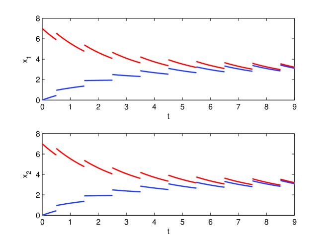
Figure 2: Transient behavior of the recurrent neural networks for the system (5.42) with the initial points $[0,0]^{T}$ and $[7,7]^{T}.$

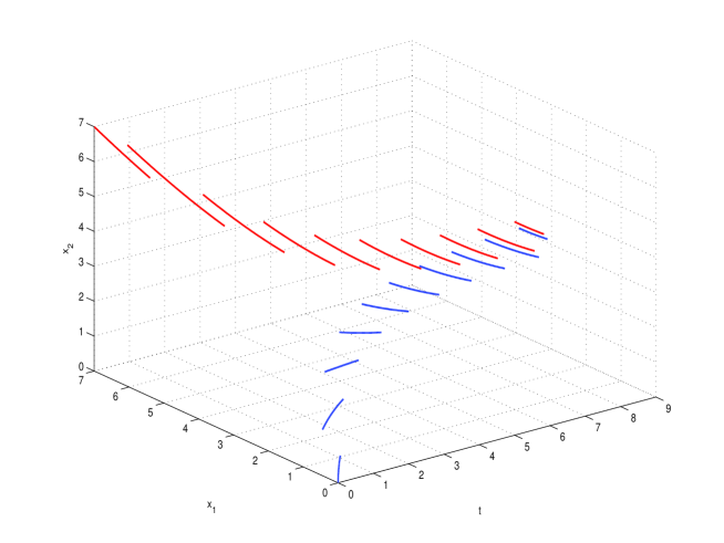
Figure 3: Eventually 1-periodic solutions of system (5.42) with the initial points $[0,0]^{T}$ and $[7,7]^{T}.$

On the other hand, in the following example, we illustrate a globally stable equilibrium appearance for our system of differential equations:

$$\left\{\begin{array}[]{lll}\frac{dx(t)}{dt}&=&-\left(\begin{array}[]{ccc}5\times 10^{-1}&0\\ 0&5\times 10^{-1}\end{array}\right)\left(\begin{array}[]{ccc}x_{1}(t)\\ x_{2}(t)\end{array}\right)+\left(\begin{array}[]{ccc}10^{-4}&\ 2\times 10^{-3}\\ 10^{-4}&3\times 10^{-3}\end{array}\right)\left(\begin{array}[]{ccc}\tanh(\frac{x_{1}(t)}{10})\\ \tanh(\frac{3x_{2}(t)}{10})\end{array}\right)\\ &&+\left(\begin{array}[]{ccc}2\times 10^{-2}&3\times 10^{-2}\\ 3\times 10^{-2}&5\times 10^{-2}\end{array}\right)\left(\begin{array}[]{ccc}\tanh(\frac{x_{1}(\beta(t))}{5})\\ \tanh(\frac{x_{2}(\beta(t))}{5})\end{array}\right)+\left(\begin{array}[]{ccc}1\\ 1\end{array}\right),\ t\neq\tau_{k}\\ \Delta x(t)&=&\left(\begin{array}[]{ccc}I(x_{1}(\tau_{k}^{-}))\\ I(x_{2}(\tau_{k}^{-}))\end{array}\right)=\left(\begin{array}[]{ccc}\frac{(x_{1}(\tau_{k}^{-})-x_{1}^{*})^{2}}{30}\\ \frac{(x_{2}(\tau_{k}^{-})-x_{1}^{*})^{2}}{30}\end{array}\right),\ t=\tau_{k},\quad k=1,2,\cdots,\end{array}\right.$$ (5.64)

where $x_{1}^{*}=2.0987,\ x_{2}^{*}=2.1577.$ One can check that the point $x^{*}=(x_{1}^{*},x_{2}^{*})$ satisfies the algebraic system

$$-a_{i}x_{i}^{*}+\displaystyle\sum_{j=1}^{2}b_{ij}f_{j}(x_{j}^{*})+\sum_{j=1}^{2}c_{ij}g_{j}(x_{j}^{*}))+d_{i}=0,$$ (5.65)

approximately. And it is clear that $I(x_{i}^{*})=0$ for $i=\overline{1,2}.$ By simple calculation, we can see that all conditions of Theorem 2.1 are satisfied and the point $x^{*}$ is a solution of (5.65), approximately with the error, which is less than $10^{-11}$(evaluated by MATLAB).

The simulation, where the initial value is chosen as $[10,10]^{T}$ , is shown in Fig. 3 and it illustrates that all trajectories converge to $x^{*}.$

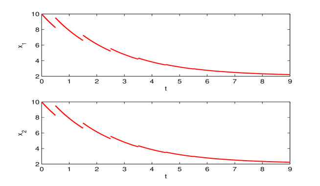
Figure 4: The first and the second coordinates of the solution for the the system (5.64) with the initial point $[10,10]^{T}$ approaches $x_{1}^{*}$ and $x_{2}^{*}$, respectively, as time increases.

Now, let us take the parameters so that the non-smoothness can also be seen. Consider the following recurrent neural networks with non-smooth and impact activations:

$$\left\{\begin{array}[]{lll}\frac{dx(t)}{dt}&=&-\left(\begin{array}[]{ccc}20&0\\ 0&8\end{array}\right)\left(\begin{array}[]{ccc}x_{1}(t)\\ x_{2}(t)\end{array}\right)+\left(\begin{array}[]{ccc}10&\ 3\\ 5&1\end{array}\right)\left(\begin{array}[]{ccc}\tanh(x_{1}(t))\\ \tanh(x_{2}(t))\end{array}\right)\\ &&+\left(\begin{array}[]{ccc}20&1\\ 8&1\end{array}\right)\left(\begin{array}[]{ccc}\tanh(x_{1}(\beta(t)))\\ \tanh(x_{2}(\beta(t)))\end{array}\right)+\left(\begin{array}[]{ccc}1\\ 1\end{array}\right),\ t\neq\tau_{k}\\ \Delta x(t)&=&\left(\begin{array}[]{ccc}I_{k}(x_{1}(\tau_{k}^{-}))\\ I_{k}(x_{2}(\tau_{k}^{-}))\end{array}\right)=\left(\begin{array}[]{ccc}\frac{x_{1}(\tau_{k}^{-})}{3}+\frac{1}{6}\\ \frac{x_{2}(\tau_{k}^{-})}{3}+\frac{1}{6}\end{array}\right),\ t=\tau_{k},\quad k=1,2,\cdots,\end{array}\right.$$ (5.87)

Clearly, one can see that our parameters are big now. Therefore, the system of equations (5.87) does not satisfy the conditions of the theorems. However, we can see the non-smoothness of the solution with the initial value $[0,0]^{T},$ which is illustrated by simulations in Fig.3. and Fig.4.

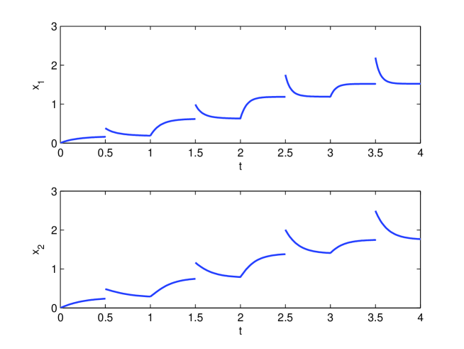
Figure 5: The impact and non-smoothness are seen at discontinuity points $\tau_{k}\ (0.5;1.5;2.5;3.5)$ and at switching points $\theta_{k}\ (1;2;3),$ respectively.

Figure 6: Eventually 1-periodic solutions of system (5.87) with the initial point $[0,0]^{T}.$

6 Conclusions

This is the first time that global asymptotic stability of periodic solutions for recurrent neural networks with both impulses and piecewise constant delay is considered. Furthermore, our model gives new ideas not only from the implementation point of view, but also from the system of differential equations. In other words, we develop differential equations with piecewise constant argument to a new class of system, so called impulsive differential equations with piecewise constant delay. For applications, we have also nice properties on the system of equations that the moments of discontinuity $\tau_{k}$ and switching moments of constancy of arguments $\theta_{k}$ are not related to each other. That is, our investigations are more applicable to the real world problems like recurrent neural networks. Finally, the results given in this paper could be developed for more complex systems [10].

References

- [1] M. Akhmet, Principles of Discontinuous Dynamical Systems, Springer, New York, 2010.
- [2] M. Akhmet, Nonlinear Hybrid Continuous/Discrete Time Models, Atlantis Press, Amsterdam-Paris, 2011.
- [3] M. U. Akhmet, On the integral manifolds of the differential equations with piecewise constant argument of generalized type, Proceedings of the Conference on Differential and Difference Equations at the Florida Institute of Technology, August 1-5, 2005, Melbourne, Florida, Editors: R.P. Agarwal and K. Perera, Hindawi Publishing Corporation, (2006) 11-20.
- [4] M. U. Akhmet, On the reduction principle for differential equations with piecewise constant argument of generalized type, J. Math. Anal. Appl. 336 (2007) 646-663.
- [5] M. U. Akhmet, Stability of differential equations with piecewise constant arguments of generalized type, Nonlinear Analysis 68 (2008) 794-803.
- [6] M. U. Akhmet and D. Aruğaslan, Lyapunov-Razumikhin method for differential equations with piecewise constant argument, Discrete Cont. Dyn. S., 25:2 (2009) 457-466.
- [7] M. U. Akhmet, D. Aruğaslan and E. Yılmaz, Stability in cellular neural networks with a piecewise constant argument, J. Comput. Appl. Math., 233, 2010 2365-2373.
- [8] M. U. Akhmet and E. Yılmaz, Impulsive Hopfield-type neural networks system with piecewise constant argumet, Nonlinear Anal: Real World Applications, 11 (2010) 2584-2593.
- [9] M. U. Akhmet, D. Aruğaslan and E. Yılmaz, Stability analysis of recurrent neural networks with piecewise constant argument of generalized type, Neural Networks, 23 (2010) 805-811.
- [10] M. U. Akhmet, Dynamical synthesis of quasi-minimal sets, International Journal of Bifurcation and Chaos, Vol. 19, No. 7 (2009), 1-5.
- [11] A. M. Samoilenko and N.A. Perestyuk, Impulsive Differential Equations, World Scientifc, Singapore, 1995.
- [12] V. Lakshmikantham, D.D. Bainov and P.S. Simeonov, Theory of Impulsive Differential Equations, in: Series in Modern Applied Mathematics, vol. 6, World Scientific, Singapore, 1989.
- [13] S. Haykin, Neural Networks: A comprehensive Foundations, Second edition, Tsinghua Press, Beijing, 2001.
- [14] J. F. Kolen and S. C. Kremer, A Field Guide to Dynamical Recurrent Networks, IEEE Press, New York, 2001.
- [15] H. Huang, D. W. C. Hob and J. Cao, Analysis of global exponential stability and periodic solutions of neural networks with time-varying delays, Neural Networks 18 (2005) 161-170.
- [16] S. Townley, A. Ilchmann, M. G. Weib, W. Mcclements, A. C. Ruiz, D. H. Owens and D. Pratzel-Wolters, Existence and learning of oscillations in recurrent neural networks, IEEE Transactions on Neural Networks, 11 (1) (2000) 205-214.
- [17] J. J. Hopfield, Neurons with graded response have collective computational properties like those of two-stage neurons, Proc. Nat. Acad. Sci. Biol. 81 (1984) 3088-3092.
- [18] J. J. Hopfield, Neural networks and physical systems with emergent collective computational abilities, Proc. Nat. Acad. Sci. Biol. 71 (1982) 2554-2558.
- [19] M. A. Cohen and S. Grossberg, Absolute stability of global pattern formation and parallel memory storage by competitive neural networks, IEEE Transactions SMC-13, pp. 815-826, 1983.
- [20] L. O. Chua and L. Yang, Cellular neural networks: Theory, IEEE Trans. Circuits Syst. 35 (1988) 1257-1272.
- [21] L. O. Chua and L. Yang, Cellular neural networks: Applications, IEEE Trans. Circuits Syst. 35 (1988) 1273-1290.
- [22] L. O. Chua and T. Roska, Cellular neural networks with nonlinear and delay type template elements and non-uniform grids, International Journal of Circuit Theory and Applications 20 (1992) 449-451.
- [23] A. N. Michel, J.A. Farrell and W. Porod, Qualitative analysis of neural networks, IEEE Trans. Circuits Systems 36 (1989) 229-243.
- [24] P. P. Civalleri, M. Gilli and L. Pandolfi, On stability of cellular neural networks with delay, IEEE Trans. Circuits Syst. I (40) (1993) 157-164.
- [25] S. Coombes and C. Laing, Delays in activity-based neural networks, Phil. Trans. R. Soc. A 2009 367, 1117-1129.
- [26] K. Gopalsamy, Stability of artificial neural networks with impulses, Appl. Math. Comput., 154 (2004) 783-813.
- [27] S. Mohammad, Exponential stability in Hopfield-type neural networks with impulses, Chaos Solitons and Fractals 32 (2007) 456-467.
- [28] Z. H. Guan, J. Lam and G. Chen , On impulsive autoassociative neural networks, Neural Networks 13 (2000) 63-9.
- [29] Z. H. Guan and G. Chen , On delayed impulsive Hopfield neural networks, Neural Networks 12 (1999) 273-280.
- [30] D. Xu and Z. Yang, Impulsive delay differential inequality and stability of neural networks, J. Math. Anal. Appl. 305 (2005) 107-120.
- [31] Y. Zhang and J. Sun, Stability of impulsive neural networks with time delays, Phys. Lett. A 348 (2005) 44-50.
- [32] Y. Yang and J. Cao, Stability and periodicity in delayed cellular neural networks with impulsive effects, Nonlinear Analysis: Real World Applications 8 (2007) 362-374.
- [33] Y. Timofeeva, Travelling waves in a model of quasi-active dendrites with active spines, Physica D 239 (2010) 494-503.
- [34] S. Coombes and P.C. Bressloff, Solitary waves in a model of dendritic cable with active spines, SIAM J. Appl. Math. 61 (2) (2000) 432-453.
- [35] Y. Liu, Z. Wang and X. Liu, Asymptotic stability for neural networks with mixed time-delays: The discrete-time case, Neural Networks 22 (2009) 67-74.
- [36] Y. Liu , Z. Wang , A. Serrano and X. Liu , Discrete-time recurrent neural networks with time-varying delays: Exponential stability analysis, Physics Letters A 362 (2007) 480-488.
- [37] N. E. Barabanov and D. V. Prokhorov, Stability analysis of discrete-time recurrent neural networks. IEEE Trans. Neural Networks 13(2) (2002) 292-303.
- [38] J. Liang, J. Cao and J. Lam, Convergence of discrete-time recurrent neural networks with variable delay, Internat. J. Bifur. Chaos 15 (2005) 581-595.
- [39] X. Zhao, Global exponential stability of discrete-time recurrent neural networks with impulses, Nonlinear Analysis 71 (2009) e2873-e2878.
- [40] S. Mohamad, Global exponential stability in continuous-time and discrete-time delayed bidirectional neural networks, Physica D 159 (2001) 233-251.
- [41] E. Yucel and S. Arik, New exponential stability results for delayed neural networks with time varying delays, Physica D, 191 (2004) 314-322.
- [42] J. Cao, Global stability analysis in delayed cellular neural networks. Physical Review E, 59, (1999) 5940-5944.
- [43] J. D. Cao and D. M. Zhou, Stability analysis of delayed cellular neural networks, Neural Networks, 11, (1998) 1601 1605.
- [44] X. M. Li, L. H. Huang and H. Y. Zhu, Global stability of cellular neural networks with constant and variable delays. Nonlinear Analysis, 53, (2003) 319-333.
- [45] S. Xu , Y. Chu and J. Lu, New results on global exponential stability of recurrent neural networks with time-varying delays, Phys. Lett. A 352 (2006) 371-379.
- [46] H. Huang, J. Cao and J. Wang, Global exponential stability and periodic solutions of recurrent neural networks with delays, Phys. Lett. A 298 (2002) 393-404.
- [47] P. V. D. Driessche and X. Zou, Global attractivity in delayed Hopfield neural network models, SIAM J. Appl. Math. Vol. 58 No. 6 (1998) 1878-1890.
- [48] Z. G. Zeng and J. Wang, Improved conditions for global exponential stability of recurrent neural networks with time-varying delays, IEEE Trans. Neural Networks 17 (3) (2006) 623-635.
- [49] K. L. Cooke and J. Wiener, Retarded differential equations with piecewise constant delays, J. Math. Anal. Appl. 99 (1984) 265-297.
- [50] J. Wiener, Generalized Solutions of Functional Differential Equations, World Scientific, Singapore, 1993.