Non-Gaussian halo abundances in the excursion set approach with correlated steps

Abstract

We study the effects of primordial non-Gaussianity on the large scale structure in the excursion set approach, accounting for correlations between steps of the random walks in the smoothed initial density field. These correlations are induced by realistic smoothing filters (as opposed to a filter that is sharp in $k$-space), but have been ignored by many analyses to date. We present analytical arguments – building on existing results for Gaussian initial conditions – which suggest that the effect of the filter at large smoothing scales is remarkably simple, and is in fact identical to what happens in the Gaussian case: the non-Gaussian walks behave as if they were smooth and deterministic, or “completely correlated”. As a result, the first crossing distribution (which determines, e.g., halo abundances) follows from the single-scale statistics of the non-Gaussian density field – the so-called “cloud-in-cloud” problem does not exist for completely correlated walks. Also, the answer from single-scale statistics is simply one half that for sharp-$k$ walks.

We explicitly test these arguments using Monte Carlo simulations of non-Gaussian walks, showing that the resulting first crossing distributions, and in particular the factor 1/2 argument, are remarkably insensitive to variations in the power spectrum and the defining non-Gaussian process. We also use our Monte Carlo walks to test some of the existing prescriptions for the non-Gaussian first crossing distribution. Since the factor 1/2 holds for both Gaussian and non-Gaussian initial conditions, it provides a theoretical motivation (the first, to our knowledge) for the common practice of analytically prescribing a ratio of non-Gaussian to Gaussian halo abundances.

1 Introduction

The detection of primordial non-Gaussianity (NG) (Maldacena 2003; Acquaviva et al. 2003) would serve as a powerful discriminator between models for seeding curvature inhomogeneities in the early universe (Babich, Creminelli & Zaldarriaga 2004; LoVerde et al. 2008; Sartoris et al. 2010; Sefusatti 2009; see Desjacques & Seljak 2010 for a recent review). Traces of primordial NG can potentially be found not only in the cosmic microwave backround (CMB) radiation (Creminelli et al. 2006; Komatsu et al. 2010), but also in the late time large scale structure of the universe (Slosar et al. 2008). Both the abundance of collapsed objects (halos) and correlations in their spatial distribution are sensitive to the presence of NG in the initial conditions (see, e.g., Dalal et al. 2008; Matarrese & Verde 2008; Afshordi & Tolley 2008). Collapsed objects and the CMB probe very different spatial scales, and the study of the former therefore promises to complement the information gained on primordial NG from the latter. Since detailed studies of collapse and structure formation involve expensive numerical simulations, it is interesting to explore the extent to which one can gain analytical insight into the problem.

The excursion set approach (Epstein 1983; Bond et al. 1991; Lacey & Cole 1993) has gone a long way in helping to build such insight. This approach simplifies the problem of structure formation by separating its highly non-linear, dynamical aspects from its statistical ones. The key idea which the approach hinges on is the realisation that matter does not move very far while halos form. This allows the problem of the late time distribution of matter, to be mapped onto its initial conditions. Whether or not a structure forms on a given length scale is decided by asking whether or not the initial density field, smoothed on that scale, lies above a certain threshold (Press & Schechter 1974). The density field performs a random walk as the smoothing scale is changed. The excursion set ansatz relates the statistics of these random walks to those of large scale structure (e.g., halo abundances, bias, merger rates, formation times, etc.), while the dynamics enters through the choice of the threshold, which acts as an absorbing barrier for the walks. Most importantly for the present discussion, the mapping of the problem onto the initial conditions brings primordial NG into the fold of the excursion set approach.

Halo abundances – the focus of this paper – in the excursion set approach are prescribed in terms of the first crossing distribution (absorption rate) of a barrier, by the random walks performed by the smoothed density field. If ${\rm d}n/{\rm d}m$ is the differential number density of halos with mass in $(m,m+{\rm d}m)$, then

$$\frac{m}{\bar{\rho}}\frac{{\rm d}n(m)}{{\rm d}m}{\rm d}m=f(s)\,{\rm d}s.$$ (1)

where $\bar{\rho}$ is the mean matter density of the universe, $s$ is the variance of the density field on scale $R$ with $m=4\pi\bar{\rho}R^{3}/3$, and $f(s)$ is the first crossing distribution. In the context of Gaussian initial conditions, it was recognised early on (Bond et al. 1991) that the first crossing distribution $f(s)$ admits an analytical solution when the field is smoothed with a filter that is sharp in $k$-space, while the problem is much more involved with a more realistic choice of filter, such as, e.g., a TopHat in real space. While Bond et al. presented numerical results (which we discuss below), it is worth noting that Peacock & Heavens (1990) had already presented an analytical approximation to the first crossing distribution of filtered walks, which described the numerical results of Bond et al. remarkably accurately.

Based on Eq. (1), it certainly appears desirable to calculate a first cross distribution, rather than perform an analysis analogous to Press & Schechter (1974) by only calculating unconditional probabilities for the smoothed density contrast to be above threshold (although see below). In the context of non-Gaussian initial conditions, however, the technical hurdles involved have meant that several analyses have relied on extending the original Press-Schechter argument to the non-Gaussian case (Matarrese, Verde & Jimenez 2000; LoVerde et al. 2008; LoVerde & Smith 2011). Only recently have there been systematic efforts to tackle the problem using the full excursion set approach of Bond et al. (e.g., Lam & Sheth 2009; Maggiore & Riotto 2010; D’Amico et al. 2011a), very few of which have explicitly addressed the issue of non-sharp-$k$ filtering (e.g., Maggiore & Riotto 2010, who work with the TopHat filter).

One issue which has hampered the understanding of non-Gaussian halo abundances, is the fact that even for Gaussian initial conditions, both types of analyses (Press-Schechter and Bond et al.) are known not to describe well the results of $N$-body simulations. In part this is because the exponential tail of the halo mass function is not well described by the canonical threshold value $\delta_{c}=1.686$ from spherical collapse (Gunn & Gott 1972), a point we will return to later. The standard practice in the literature has therefore been to use Press-Schechter/sharp-$k$ analyses to prescribe a ratio $R_{\rm NG}=f_{\rm NG}/f_{\rm gauss}$ (e.g. LoVerde et al. 2008). As yet, there has been no convincing explanation of why such a prescription can be expected to work, although $N$-body simulations with non-Gaussian initial conditions indicate that the prescription does work (Grossi et al. 2007; Pillepich, Porciani & Hahn 2008; Desjacques & Seljak 2010). And finally, it is also worth keeping in mind that equating the halo abundances on the left hand side of Eq. (1) with the first crossing distribution on the right, is only an ansatz (see Paranjape, Lam & Sheth 2011a, henceforth PLS11, for a discussion).

Overall then, the present situation as regards the non-Gaussian halo mass function is, in our opinion, rather clouded. There are several calculations of the function $f_{\rm NG}(s)$ which appears on the right hand side of Eq. (1). Accepting that $f_{\rm NG}(s)$ must be a first crossing distribution, we see that none of the calculations of $f_{\rm NG}(s)$ have been tested using numerical first crossing distributions. Consequently, one cannot claim to understand which (if any) prescription for $f_{\rm NG}(s)$ works well. The ratio prescription has been tested in $N$-body simulations and seems to do well; however, as yet there is no theoretical understanding of why this must be so. There have been very few attempts to assess the impact of nontrivial filtering on the calculation of $f_{\rm NG}(s)$, mainly based on a linearization of the problem (Maggiore & Riotto 2010). However, since the expansion parameter involved is of order $\sim 0.4$, we would argue that the actual effect of filtering on non-Gaussian random walks is not yet clear.

Our aim in this paper is to gain some insight into these issues. We will therefore focus on testing analytical prescriptions for non-Gaussian first crossing distributions using Monte Carlo simulations of random walks (as opposed to mass functions from $N$-body simulations), along the lines initiated by PLS11 for the Gaussian case. We will demonstrate that the first crossing distribution of sharp-$k$ non-Gaussian walks on the relevant scales is rather insensitive to the exact nature of the defining non-Gaussian process, and depends, instead, mainly on the values of the leading order parameters (such as the skewness) which define the process. Our main result, however, concerns the effects of a nontrivial filter. We will present analytical arguments, supported by our numerics, to show that for small values of variance $s$ the first crossing distribution of filtered non-Gaussian walks is simply a factor $1/2$ times the corresponding distribution for sharp-$k$ walks. This effect is also remarkably robust against dramatic changes in, e.g., the power spectrum and type of non-Gaussianity. Since the same effect is known to be true for the case of Gaussian walks, as an immediate consequence we see that the ratio $f_{\rm NG}/f_{\rm gauss}$ of first crossing distributions at small $s$ is independent of the choice of filter. While this does not on its own explain the effect being seen in simulations, since there is a big leap involved in going from first crossing distributions to mass functions, we believe it at least makes the ratio prescription theoretically plausible.

The paper is organized as follows. In section 2 we present our analytical arguments, explaining the role of the filter. Section 3 deals with the numerical solution; we show results for different choices of power spectra and non-Gaussian processes. A final section summarizes and discusses some avenues for further work. The Appendix contains some technical details regarding the structure of non-Gaussianity.

2 Analytical arguments: a factor of $1/2$

The problem of evaluating the first crossing distribution of random walks with correlated steps for Gaussian initial conditions, was solved numerically by Bond et al. (1991). In the cosmological context, it is the linearly extrapolated, smoothed density field $\delta$ which performs a random walk in steps of its variance

$$s(R)=\langle\,\delta_{R}^{2}\,\rangle=\int\mathrm{d}k\,k^{2}\frac{P_{\delta}(k)}{2\pi^{2}}W^{2}(kR)\;,$$ (2)

where $P_{\delta}(k)$ is the power spectrum of matter fluctuations, linearly evolved to present day, and $W(kR)$ is a smoothing filter. While a filter that is sharp in $k$-space leads to walks with uncorrelated steps, which can be treated analytically, more realistic filters such as the TopHat (in real space) or Gaussian lead to nontrivial correlations between steps. Among other things, Bond et al.  demonstrated that the high-mass or small $s$ tail of the first crossing distribution $f(s)$ is very well described, independently of the choice of filter and power spectrum, by the Press-Schechter expression

$$sf_{\rm PS}(s)=\frac{1}{2}\frac{\delta_{c}}{\sqrt{2\pi s}}e^{-\delta_{c}^{2}/2s}\,,$$ (3)

which is a factor $1/2$ different from the analytical answer for walks with uncorrelated steps. The analytical approximation presented by Peacock & Heavens (1990) also reduces to this expression for small $s$, independently of the filter and power spectrum. In both cases, the actual details of the filter and power spectrum only come into play when the relation between $s$ and the smoothing scale $R$ is needed.

This behaviour can be understood in terms of what PLS11 recently discussed as the “completely correlated” limit of the random walks. In this limit, the walks are deterministic in the sense that each walk has a constant value of $\nu=\delta/\sqrt{s}$. In the plane of $\delta/\sqrt{s}$ vs. $s$, each walk therefore crosses the barrier $\delta=\delta_{c}$ at most once. The “survival probability”, i.e. the fraction of walks that has not crossed at $s$, is therefore simply the fraction of walks for which $\nu<\delta_{c}/\sqrt{s}$, which is $(1+{\rm erf}(\delta_{c}/\sqrt{2s}))/2$ for Gaussian initial conditions. The derivative of this survival probability leads to the Press-Schechter expression (3), which is therefore the first crossing distribution for walks with completely correlated steps and Gaussian initial conditions.

In other words, the so-called cloud-in-cloud problem which Bond et al. solved for the sharp-$k$ case, does not exist for completely correlated walks; such walks either cross the constant barrier exactly once, or not at all. For correlations induced by realistic filters (such as the TopHat or Gaussian), Eq. (3) remains a good description at small $s$, since the walks have not had enough “time” to start feeling the effects of stochasticity; in the small $s$ limit, the walks are still completely correlated.

Now consider the case of non-Gaussian initial conditions. In what follows it will be useful to define the normalised equal-scale connected moments of the non-Gaussian field $\delta$, $\epsilon_{j}\equiv\langle\,\delta^{j+2}\,\rangle_{c}/s^{(j+2)/2}$, the most important for us being the three-point function given by $\epsilon_{1}$,

$$\epsilon_{1}\equiv\frac{\langle\,\delta^{3}(s)\,\rangle}{s^{3/2}}\,.$$ (4)

A recent analysis by Maggiore & Riotto (2010) has explored TopHat filter effects in the calculation of the first crossing distribution, using a path-integrals analysis. In contrast, we will be guided by the discussion above of the case of Gaussian initial conditions. In particular, for small $s$ that entire argument goes through as is for the non-Gaussian case as well, apart from the fact that, at any given $s$, the fraction of walks $P_{\rm NG}(<\delta_{c}/\sqrt{s})$ with $\nu<\delta_{c}/\sqrt{s}$ is no longer simply an error function, but receives non-Gaussian corrections. These corrections, however, can be calculated simply by knowing the single-point statistics of the non-Gaussian filtered field $\delta$, even though this field in general has a complicated structure of unequal-scale correlations. This happens because, as far as the tail of the first crossing distribution is concerned, any memory induced by the non-Gaussianity is rendered superfluous by these filter-induced strong correlations. We check this explicitly in the next section, by numerically calculating the first crossing distribution of non-Gaussian walks.

To summarize, we have argued that in its small $s$ tail the first crossing distribution of walks with non-Gaussian initial conditions and filter-induced correlated steps must be the derivative of the survival probability for walks with completely correlated steps:

$$sf_{\rm NG}(s)=-s\frac{\partial}{\partial s}P_{\rm surv}(s)\to-s\frac{\partial}{\partial s}P_{\rm NG}(<\delta_{c}/\sqrt{s})\,.$$ (5)

We emphasize that the final result is valid only for small $s$; the result for Gaussian initial conditions (Peacock & Heavens 1990; Bond et al. 1991) suggests that the shape of the distribution at large $s$ could be very different. This is not a major concern, since the effect of primordial non-Gaussianity is expected to be large only at small $s$, and consequently we need not worry about deviations from this simple result at large $s$.

This final result is not new in itself; the single-point statistics of the non-Gaussian field have been the basis of the calculations of, e.g., Matarrese, Verde & Jimenez (2000) (henceforth MVJ00), LoVerde et al. (2008) and LoVerde & Smith (2011). However, since those analyses ultimately aimed at obtaining a mass function rather than a first crossing distribution, the true statistical meaning of those calculations has become clouded, in our opinion, and is clarified by our arguments above.

It is worth comparing the structure of the sharp-$k$ non-Gaussian first crossing distribution with that of the unconditional probability $P_{\rm NG}(<\delta_{c}/\sqrt{s})$ in some detail, since this yields some insight into the ratio prescription mentioned in the Introduction. The calculation of Maggiore & Riotto (2010) shows that the effect of unequal scale correlations of the non-Gaussian field $\delta$ in the first crossing distribution, are typically suppressed by powers of $\nu^{-1}=\sqrt{s}/\delta_{c}$ in the small $s$ tail. As we explain below, if we therefore ignore these contributions altogether, then the derivative with respect to $s$ of the probability $P_{\rm NG}(<\delta_{c}/\sqrt{s})$, when expressed in terms of the equal-scale connected moments $\epsilon_{j}$, will be exactly $1/2$ times the sharp-$k$ first crossing distribution,

$$-s\frac{\partial}{\partial s}P_{\rm NG}(<\delta_{c}/\sqrt{s})=\frac{1}{2}\times sf_{{\rm NG,sharp-}k}(s)\,.$$ (6)

The reason is that in each case, sharp-$k$ as well as completely correlated, the non-Gaussianity appears as an exponentiated derivative operator $\sim\exp[-\epsilon_{1}\partial_{\nu}^{3}/6+\ldots]$ acting on the corresponding Gaussian first crossing distribution. This can be seen, e.g., by comparing equation (A3) of Paranjape, Gordon & Hotchkiss (2011) (henceforth PGH11) for the sharp-$k$ case, with equations (26) and (36) of MVJ00 for the completely correlated case.

The theoretical effort now lies in computing the effect of this derivative operator, and different groups have approached the problem with different assumptions (see e.g. MVJ00, LoVerde et al. 2008, Maggiore & Riotto 2010, D’Amico et al. 2011a, PGH11). The bottom-line for us is the same in each case: since the Gaussian results for the sharp-$k$ and completely correlated cases differ by a factor of $1/2$, consequently so do the non-Gaussian answers. An immediate consequence is that at small $s$, the ratio of non-Gaussian to Gaussian first crossing distributions $f_{\rm NG}/f_{\rm gauss}$ will be the same regardless of whether the walks were sharp-$k$ filtered or, more realistically, completely correlated.

As with the case of Gaussian initial conditions, the relation between $s$ and smoothing scale $R$ explicitly depends on the choice of filter and power spectrum. Additionally now, the moments $\epsilon_{j}$ will also in general be sensitive to these choices. What is universal though, is the functional form of the right hand side of Eq. (6) when expressed in terms of $s$ and the $\epsilon_{j}$.

For later comparison, we note here that the completely correlated prediction derived from the PGH11 prescription reads (with $\nu\equiv\delta_{c}/\sqrt{s}$)

$$sf_{\rm PGH,cc}(s)= \frac{1}{2}\frac{\nu}{\sqrt{2\pi(1+\epsilon_{1}\nu)}}$$

$$\phantom{\frac{1}{2}}\times\exp\left[\frac{\epsilon_{1}\nu-(1+\epsilon_{1}\nu)\ln(1+\epsilon_{1}\nu)}{\epsilon_{1}^{2}}\right]\,,$$ (7)

while the corresponding prediction for MVJ00 is

$$sf_{\rm MVJ,cc}(s)=\frac{1}{2}\frac{\nu}{\sqrt{2\pi(1-\frac{1}{3}\epsilon_{1}\nu)}}e^{-\frac{1}{2}\nu^{2}(1-\frac{1}{3}\epsilon_{1}\nu)}\left(1-\frac{1}{2}\epsilon_{1}\nu\right)\,,$$ (8)

in which we assumed $\epsilon_{1}$ to be constant, which is what we will use for our numerical results below.

3 Monte Carlo tests

To verify that filter-induced correlations do in fact completely correlate the walks at small $s$, in this subsection we numerically calculate the first crossing distributions for non-Gaussian random walks, comparing the effect of sharp-$k$ and Gaussian filters. The results are not expected to change when switching to the TopHat filter; we choose the Gaussian filter since it allows us to derive simple analytical expressions for some of the quantities we will need below. Along the way we will also demonstrate that, for the sharp-$k$ walks as well, the first crossing distribution is rather insensitive to the details of the unequal scale correlations of the non-Gaussian field.

3.1 Gaussian initial conditions

Figure 1: Distribution of scale $s$ at which a walk first crossed the constant barrier $\delta=\delta_{c}$ (histograms), for sharp-$k$ (solid) and Gaussian filtered (dashed) walks with Gaussian initial conditions. While the filtered walks assumed a power law power spectrum $P_{\delta}(k)\propto k^{-1.2}$, the result is insensitive to the choice of $P_{\delta}(k)$. The histograms agree with the analytical predictions (smooth curves) of Bond et al. (1991) (solid) and Eq. (3) (dashed), respectively.

To set the stage, let us begin by discussing the case of Gaussian initial conditions in some detail. The strategy for generating walks with Gaussian initial conditions is the same as that employed by Bond et al. (1991): the sharp-$k$ walks are constructed by accumulating independent Gaussian random numbers $g_{i}$ with a fixed variance $\Delta s$, $\delta_{j}^{({\rm sharp-}k)}=\sum_{i=1}^{j}g_{i}$, while the Gaussian filtered walks are obtained by applying the filter $W(kR)=e^{-(kR)^{2}/2}$ to the same set of numbers to get $\delta_{j}^{\rm(Gau)}=\sum_{i}g_{i}W(k_{i}R_{j})$. In the latter case, one also needs to know which values of $k_{j}$ and $R_{j}$ to associate to the $j$-th step. Once a power spectrum is specified, this can be done by inverting the relations $j\Delta S=(2\pi^{2})^{-1}\int_{0}^{k_{j}}\mathrm{d}k\,k^{2}P_{\delta}(k)$ and $j\Delta S=(2\pi^{2})^{-1}\int_{0}^{+\infty}\mathrm{d}k\,k^{2}P_{\delta}(k)W^{2}(kR_{j})$.

In this work, we will use a power law form $P_{\delta}(k)\propto k^{n}$ for the power spectrum, rather than the $\Lambda$CDM form, in order to simplify the analysis. The results of Bond et al., and our previous analytical arguments, suggest that the final result for the non-Gaussian first crossing distribution should be independent of the form of the power spectrum. We will also explicitly verify this expectation by displaying results for two very different values of $n$. As a sanity check, the histograms in Figure 1 show our numerical solution for the first crossing distribution of the constant barrier $\delta=\delta_{c}$ for walks with Gaussian initial conditions, for the sharp-$k$ and Gaussian filters respectively, with $n=-1.2$. The corresponding smooth curves show the analytical expressions of Bond et al. (1991) and Eq. (3), respectively, which differ by a factor $1/2$. The agreement indicates that our code is working correctly.

3.2 Non-Gaussian initial conditions: model definitions

To generate non-Gaussian walks, we must choose a type of non-Gaussianity. Ideally, we would pick as the initial density field a realization of a non-Gaussian process compatible with the bispectrum shape of some specific model of inflation, and smooth it with the filter of choice to obtain the walks. For example, in the so-called local model (Komatsu & Spergel 2001; Lyth, Ungarelli & Wands 2003; Bartolo, Matarrese & Riotto 2004; Dvali, Gruzinov & Zaldarriaga 2004) the primordial curvature perturbation $\zeta(\vec{x})$ is written in real space as $\zeta\sim\zeta_{G}+f_{\rm NL}\zeta_{G}^{2}$, where $\zeta_{G}$ is a Gaussian random field. The density contrast $\delta$ is then obtained from $\zeta$ applying the Poisson equation and some matter transfer function.

In practice, however, the nonlinear part of this $\delta$ involves a convolution in Fourier space over the modes of a Gaussian field $\delta_{G}$, which is somewhat cumbersome to handle. Since our goal is mainly to demonstrate the effect of the filter (namely, the factor of $1/2$ in the first crossing distribution), it is sufficient to adopt a simpler model. Our main requirement will be that our model must reproduce an equal-scale three point function $\epsilon_{1}$ of our choice. In the local model, $\epsilon_{1}$ is weakly scale dependent; for our numerical walks, we will simply choose a constant value for $\epsilon_{1}$. Additionally, we will also consider specific choices of unequal-scale behaviour for the three-point function. We discuss the unequal scale behaviour of the three-point function of the local model, in Appendix A1.

We will consider the class of integrated non-Gaussian processes defined by

$$\delta(S) =\delta_{G}(S)+\frac{\beta(S)}{3}\!\int_{0}^{S}\!\mathrm{d}s\frac{\delta_{G}(S)\dot{\delta}_{G}(s)-\langle\,\!\delta_{G}(S)\dot{\delta}_{G}(s)\!\,\rangle}{\gamma(s)},$$ (9)

where $\delta_{G}$ is the Gaussian field smoothed with the filter of choice, the dot is a derivative with respect to the argument $s$, and $\beta$ and $\gamma$ are functions that can be tuned to reproduce the desired behavior of the three-point function. As we show in Appendix A2, setting

$$\beta(S)=\epsilon_{1}\sqrt{S}\bigg{[}2\int_{0}^{S}\!\mathrm{d}s\frac{\langle\,\!\delta_{G}(S)\dot{\delta}_{G}(s)\!\,\rangle}{\gamma(s)}\bigg{]}^{-1}$$ (10)

allows us to match exactly any value of $\epsilon_{1}$, for any choice of filter. This expression for $\beta(S)$ ignores corrections from a term involving $\epsilon_{1}^{3}$; we have checked that, for the values of $\epsilon_{1}$ we consider in this work, including this correction does not affect any of our numerical results. For later use, note that for a sharp-$k$ filter, $\langle\,\!\delta_{G}(S)\dot{\delta}_{G}(s)\!\,\rangle=1$, while for the Gaussian filter and a power law $P_{\delta}(k)\propto k^{n}$, we have $\langle\,\!\delta_{G}(S)\dot{\delta}_{G}(s)\!\,\rangle=2^{(n+3)/2}[1+(s/S)^{2/(n+3)}]^{-(n+5)/2}$.

Additionally, setting $\gamma(s)=4\sqrt{s}$ approximately reproduces the unequal scale behavior of $\langle\,\delta(S_{1})\delta(S_{2})\delta(S_{3})\,\rangle$ of the filtered local model, and makes the model above a good proxy to study non-Gaussianity of the local type (see Appendix A2). We emphasize, however, that the details of the non-Gaussian process are actually expected to be irrelevant for the first crossing distribution. One could, e.g., pick the function $\gamma(s)$ so as to generate any other choice of unequal scale behaviour. Below, we will also display the results of simply setting $\gamma(s)=1$.

We will refer to the case $\gamma(s)=4\sqrt{s}$ as model A. When generating the random walks for this model, we find it more convenient to analytically perform an integration by parts and bring the model definition to the form

$$\delta(S) =\delta_{G}(S)+\frac{\epsilon_{1}}{6(1+\alpha)}\!\bigg{[}\frac{\delta_{G}(S)^{2}-S}{\sqrt{S}}$$

$$\phantom{\delta_{G}(S)+\epsilon_{1}(1+\alpha)}+\delta_{G}(S)\int_{0}^{S}\!\frac{\mathrm{d}s}{2s^{3/2}}\delta_{G}(s)-\alpha\sqrt{S}\bigg{]}\,,$$ (11)

where $\alpha=1$ for the sharp-$k$ filter, and for the Gaussian filter with $P_{\delta}(k)\propto k^{n}$, $\alpha=(1.52,1.31)$ for $n=(-1.2,-2)$, which follows from using the expression for $\langle\,\delta_{G}(S)\dot{}\delta_{G}(s)\,\rangle$ mentioned earlier, and performing the resulting integrals.

The second model we will consider (henceforth model B) is defined by setting $\gamma(s)=1$ in Eq. (9) and choosing $\beta$ appropriately,

$$\delta(s)=\delta_{G}(s)+\frac{\epsilon_{1}}{6}\left(\frac{\delta_{G}(s)^{2}-s}{\sqrt{s}}\right)\,,$$ (12)

(see Appendix A for details). This model significantly differs from model A, and hence from the local model as well, in the structure of the unequal scale three point function $\langle\,\delta(s_{1})\delta(s_{2})\delta(s_{3})\,\rangle$. As we show in the Appendix, in the limit when $s_{1}\ll s_{2}\ll s_{3}$, model B has $\langle\,\delta(s_{1})\delta(s_{2})\delta(s_{3})\,\rangle\propto s_{1}\sqrt{s_{2}}$ whereas the local model has $\langle\,\delta(s_{1})\delta(s_{2})\delta(s_{3})\,\rangle_{\rm loc}\propto\sqrt{s_{1}}s_{2}$.

Model B is also interesting because its single-point statistics can be calculated analytically (see, e.g., Eqs. 2-5 of MVJ00). We do this in Appendix B and show that the first crossing distribution for walks with completely correlated steps (the analog of Eqs. 3, 7 and 8) is

$$sf_{\rm NG,\,modB}(s)=\frac{1}{2}\frac{\delta_{c}}{\sqrt{s}}p_{\rm modB}\left(\frac{\delta_{c}}{\sqrt{s}},\epsilon_{1}\right)\,,$$ (13)

where, defining $\lambda(\nu,\epsilon_{1})\equiv(\epsilon_{1}/3)(\nu+\epsilon_{1}/6)$,

$$p_{\rm modB}(\nu,\epsilon_{1}) =\frac{1}{\sqrt{2\pi(1+2\lambda(\nu,\epsilon_{1}))}}\exp\left[-\frac{9}{\epsilon_{1}^{2}}(1+\lambda(\nu,\epsilon_{1}))\right]$$

$$\phantom{2\pi 2\lambda+1}\times 2\cosh\left(\frac{9}{\epsilon_{1}^{2}}\sqrt{1+2\lambda(\nu,\epsilon_{1})}\right)\,.$$ (14)

We will use this below to test our claim that single-point statistics are sufficient to determine the first crossing distribution of filtered walks.

3.3 Non-Gaussian walks: sharp-$k$ case

Our emphasis here is on the factor $1/2$ which arises due to the walks being completely correlated at small $s$. As such, it would be enough to simply display the ratio of the first crossing distributions for Gaussian filtered and sharp-$k$ walks, checking that it is consistent with being $1/2$, and we do this below. We would like to do more, however, and also compare various theoretical prescriptions for the first crossing distribution against our numerical results. Additionally, we wish to emphasize the point that the sharp-$k$ results for the first crossing distribution are also insensitive to the non-Gaussian process. We therefore show the results for sharp-$k$ separately in this subsection, with those for Gaussian filtered walks in the next subsection.

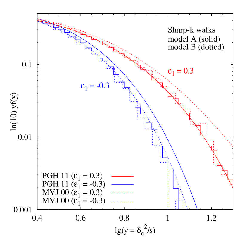
Figure 2: Distribution of scale $s$ at which a walk first crossed the constant barrier $\delta=\delta_{c}$ (histograms), for sharp-$k$ walks with non-Gaussian initial conditions defined by models A (solid) and B (dotted), for $\epsilon_{1}=0.3$ (red, upper) and $\epsilon_{1}=-0.3$ (blue, lower). Note that the histograms for the different models are remarkably alike. The smooth curves show the theoretical predictions of PGH11 (solid) and MVJ00 (dotted), with the red (upper) and blue (lower) curves corresponding to positive and negative $\epsilon_{1}$, respectively, with $|\epsilon_{1}|=0.3$ in each case. See text for a discussion.

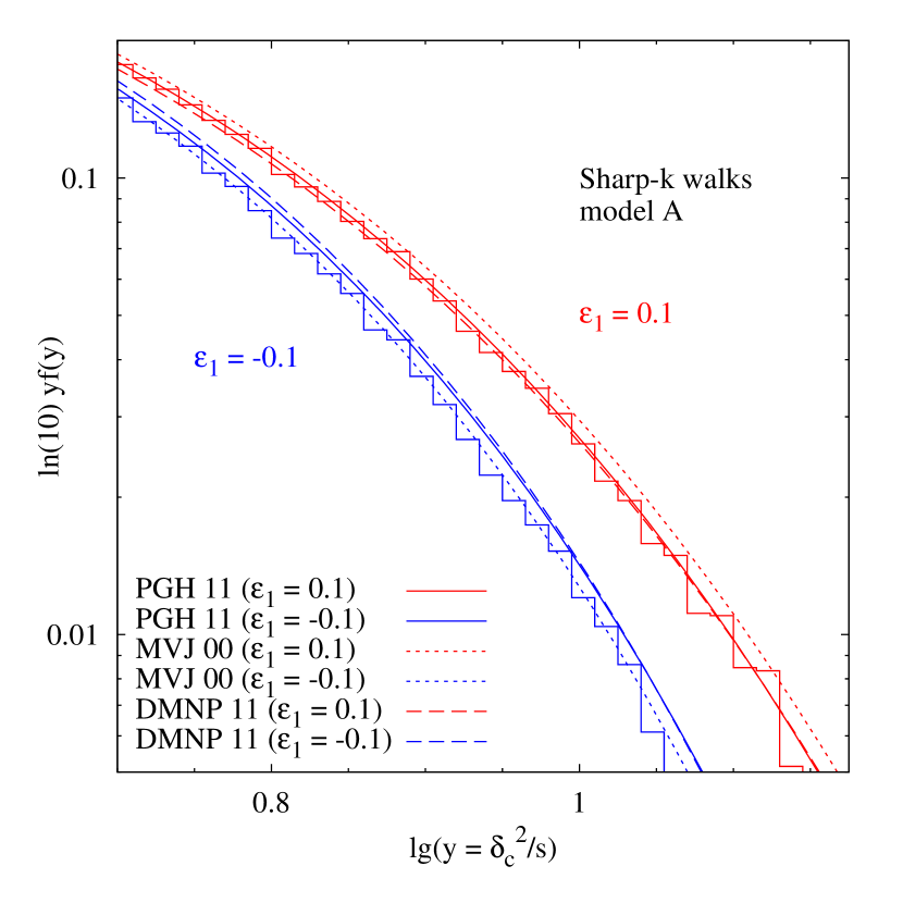
Figure 3: Same as Figure 2, but for $|\epsilon_{1}|=0.1$, with histograms shown only for model A. For this case, we also show the theoretical predictions of D’Amico et al. (2011a) as the dashed curves.

Figure 2 shows the results for $|\epsilon_{1}|=0.3$, with the red (upper) and blue (lower) histograms showing the first crossing distributions of the constant barrier $\delta=\delta_{c}$, for walks with positive and negative $\epsilon_{1}$, respectively. The solid histograms are for model A and the dotted for model B. The histograms clearly demonstrate that, within the numerical accuracy we reach, the sharp-$k$ first crossing distribution is insensitive to the details of the non-Gaussian process.

The value $|\epsilon_{1}|=0.3$ corresponds to a rather large non-Gaussianity, since e.g. in the local model one has $\epsilon_{1}\simeq 3\times 10^{-4}f_{\rm NL}$, so that in our case $|f_{\rm NL}|\sim 1000$. While we made this choice to visually enhance the effect of non-Gaussianity in the first crossing distribution, it also raises an interesting question regarding comparison with theory. As discussed elsewhere (see e.g. D’Amico et al. 2011a and PGH11), most theoretical analyses rely on a perturbative expansion in parameter combinations such as $\epsilon_{1}\nu$, and the large value $|\epsilon_{1}|=0.3$ means that these analyses break down around $\nu\lesssim 3$. The model presented in PGH11, on the other hand, was specifically constructed to remain well-defined in the tail $\nu\gg 1$ for $\epsilon_{1}>0$, and is therefore a natural choice for comparison.

The solid curves show the theory predictions from PGH11 (i.e., $2$ times the expression in Eq. (7)) for positive (red, upper) and negative (blue, lower) $\epsilon_{1}$, respectively. We see that this prescription performs remarkably well when $\epsilon_{1}>0$, while it does not do well for $\epsilon_{1}<0$. The latter is not surprising, given that the theoretical derivation of PGH11 strictly works only for $\epsilon_{1}>0$, with the $\epsilon_{1}<0$ prescription being ad hoc. The agreement for $\epsilon_{1}>0$, on the other hand, highlights once more the insensitivity of the first crossing distribution to the details of the non-Gaussianity. This is because the calculation of PGH11 assumed the relations $\epsilon_{n}=(\epsilon_{1})^{n}$, whereas in our models A and B one can check e.g. that $\epsilon_{2}\neq\epsilon_{1}^{2}$.

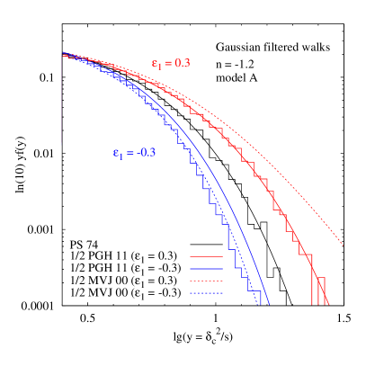
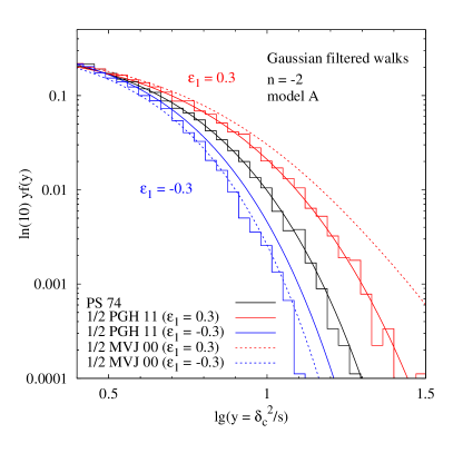
Figure 4: First crossing distribution for Gaussian filtered walks having non-Gaussian initial conditions specified by model A (histograms) and with $P_{\delta}\propto k^{n}$, with $n=-1.2$ (left panel) and $n=-2$ (right panel). The red (upper) and blue (lower) histograms show results for $\epsilon_{1}=0.3$ and $\epsilon_{1}=-0.3$, respectively. For comparison, the black (middle) histograms show the first crossing distribution for corresponding walks with Gaussian initial conditions. The smooth curves are the same in each panel. The black solid (middle) curve is the Gaussian prediction Eq. (3). The other solid curves are the non-Gaussian prediction Eq. (7), with the red (upper) and blue (lower) corresponding to $\epsilon_{1}=0.3$ and $\epsilon_{1}=-0.3$, respectively. The dotted curves similarly show the prediction Eq. (8). See text for a discussion.

The dotted curves in Figure 2 show the prediction of MVJ00 (i.e., $2$ times Eq. (8)). Given the large value of $|\epsilon_{1}|$, a priori one does not expect this prescription to be a good description of the walks, for either sign of $\epsilon_{1}$. This is quite clearly the case for $\epsilon_{1}>0$, with the dotted curve overestimating the numerical answer by a factor of $4$ or more. Remarkably, though, the MVJ00 prescription works quite well for $\epsilon_{1}<0$, although it slightly overestimates the numerical answer.

Figure 3 has the same format as Figure 2, and shows the sharp-$k$ results for a smaller value $|\epsilon_{1}|=0.1$. This time, in addition to PGH11 and MVJ00, we also show the calculation of D’Amico et al. (2011a) (dashed lines). We see that all three prescriptions perform reasonably well now, although once again the MVJ00 prescription seems to work better than the others at negative $\epsilon_{1}$. It is not clear to us whether this is indicating something deeper, or is simply a coincidence.

3.4 Non-Gaussian walks: Gaussian filtered case

We now turn to the more interesting case of filtered walks. Figure 4 has a similar format as the previous figures, and shows our results for Gaussian filtered model A walks, for the first crossing of the constant barrier $\delta=\delta_{c}$ . The red (upper) and blue (lower) histograms are for $\epsilon_{1}=\pm 0.3$ as before, while the black (middle) histogram shows the answer for Gaussian initial conditions, with the corresponding analytical prediction from Eq. (3). The two panels are for $n=-1.2$ and $-2$, and clearly the corresponding histograms do not show any significant difference from each other, highlighting the point we made earlier regarding the irrelevance of the form of the power spectrum for the completely correlated tail. We expect the same to remain true for $\Lambda$CDM as well.

The theory curves in each panel are the same; the solid curves show Eq. (7) (red, upper for $\epsilon_{1}=0.3$ and blue, lower for $\epsilon_{1}=-0.3$), while the dotted curves similarly show Eq. (8). Notice that these curves describe the histograms in each panel as well (or poorly) as the corresponding curves in Figure 2 described the sharp-$k$ non-Gaussian walks. This is a clear demonstration that the factor $1/2$ argument works extremely well in the tail of the distribution, independently of choice of power spectrum.

The histograms in Figure 5 show the results for Gaussian filtered model B walks with $n=-1.2$. For the theory curves, we only display Eq. (7) for $\epsilon_{1}>0$ (red, solid) and Eq. (8) for $\epsilon_{1}<0$ (blue,dotted). Additionally, the dashed lines show the prediction in Eq. (13) of single-point statistics for model B. The dashed lines compare extremely well with the histograms, and confirm our argument that single-point statistics are sufficient to describe the first crossing distribution of filtered walks. The good agreement between the dashed lines and the other theory curves indicates that the factor $1/2$ argument is also working well, and is moreover independent of the type of non-Gaussianity. To make this point explicitly, Figure 6 shows the ratio of the (numerical) first crossing distributions for the Gaussian filtered and sharp-$k$ walks. We see that the factor $1/2$ argument works well within our numerical accuracy. There is an order $\sim 10\%$ discrepancy at larger $s$ for the case of $n=-2$, model A (middle panel), indicating the limit until which the walks can be assumed to be completely correlated.

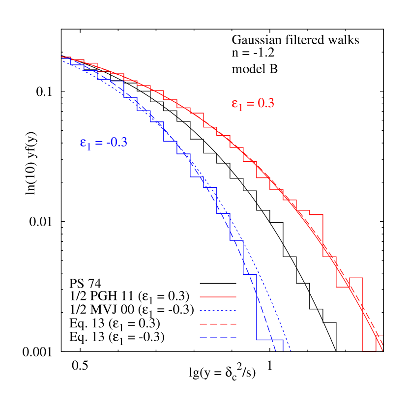
Figure 5: Same as Figure 4, but for non-Gaussian walks defined by model B, with $n=-1.2$. For the theory curves, we only display the $\epsilon_{1}>0$ prediction for Eq. (7) (solid red, upper) and the $\epsilon_{1}<0$ prediction for Eq. (8) (dotted blue, lower). Additionally, the dashed curves show the prediction of single-point statistics for model B in Eq. (13) for positive (red, upper) and negative (blue, lower) $\epsilon_{1}$, respectively, with $|\epsilon_{1}|=0.3$. See text for a discussion.

4 Discussion

An essential ingredient in the application of the excursion set approach to study structure formation from non-Gaussian initial conditions, is the ability to calculate the first crossing distribution $f_{\rm NG}(s)$ of a chosen barrier, for the random walk performed by the non-Gaussian initial density field $\delta(s)$ smoothed on a scale corresponding to variance $s$. We pointed out that, while there exist several prescriptions in the literature to calculate $f_{\rm NG}(s)$ theoretically, as yet there has been no systematic test of these prescriptions using numerically generated first crossing distributions. We have performed such tests in this work, and in the process have gained some insight into the structure of $f_{\rm NG}(s)$. We summarize our results below:

• By simulating two models of non-Gaussianity (NG) (Eqs. 11 and 12), we argued that for the case of sharp-$k$ filtering, $f_{\rm NG}(s)$ is insensitive to the exact details of the non-Gaussian process. We also showed that for small values of reduced skewness $|\epsilon_{1}|$, three different theoretical prescriptions (PGH11, MVJ00 and D’Amico et al. 2011a) work reasonably well (Figure 3), while for larger values of $|\epsilon_{1}|$, the PGH11 prescription works well for $\epsilon_{1}>0$ while the MVJ00 prescription does better for $\epsilon_{1}<0$ (Figure 2).

• For the more interesting case of filtered walks, we argued that the small $s$ tail of the first crossing distribution is essentially determined by the single-point statistics of the smoothed non-Gaussian density field. For one of our non-Gaussian models (model B) which admits a closed form analytic expression for the single-point PDF, we also explicitly verified this numerically (Figure 5).

• We further argued, and demonstrated numerically (Figures 4 and 5), that the first crossing distribution for filtered non-Gaussian walks in the limit of small $s$, is simply a factor $1/2$ times the corresponding distribution for sharp-$k$ walks. (For the numerical results, we used Gaussian filtering, but the results are not expected to change for TopHat filtering.) Since walks with Gaussian initial conditions show the same effect, this implies that the ratio $f_{\rm NG}/f_{\rm gauss}$ is independent of choice of filter, providing a theoretical motivation for the practice of prescribing such a ratio when dealing with non-Gaussian mass functions.

• We demonstrated that the previous result is remarkably robust against changing not only the power spectrum (which might have been expected based on results for Gaussian initial conditions), but also the details of the non-Gaussian process. While this probably means that halo abundances on their own will never be very sensitive to differences in types of NG, it does also reassure us that theoretical calculations can safely make assumptions regarding the non-Gaussian process (e.g., the PGH11 assumption of $\epsilon_{j}=(\epsilon_{1})^{j}$, or simply the single-point statistics of model B in Eq. (13)), without significantly affecting the final answer.

  

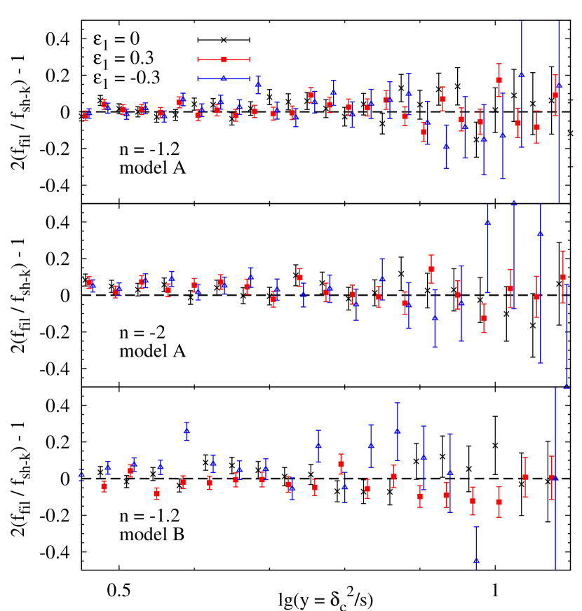
  Figure 6: Behaviour of the ratio $f_{\rm filtered}/f_{{\rm sharp-}k}$ of Gaussian filtered and sharp-$k$ first crossing distributions, relative to the predicted value of $1/2$. The three panels show various combinations of power spectrum $P_{\delta}(k)\propto k^{n}$ and non-Gaussian process as discussed in the text. The black crosses, red squares and blue triangles show the results (with Poisson errors) for $\epsilon_{1}=0$, $0.3$ and $-0.3$, respectively.

  These considerations imply that studying primordial NG in the framework of the excursion set approach is actually much simpler than sharp-$k$ analyses seem to suggest: at small $s$, the first crossing distributions of filtered walks (which are expected to be more realistic than sharp-$k$ walks) are determined entirely by the single-scale statistics of the initial density field, with no complications due to the cloud-in-cloud problem. To the extent that first crossing distributions are sufficient to study halo abundances, we would argue that, for large masses, it is both simpler and more accurate to study primordial NG using a Press-Schechter-like approach rather than the full machinery of excursion sets.

  However, as mentioned earlier, equating a first crossing distribution to a halo mass function is only an ansatz. All our results are subject to the same caveats as in the case of Gaussian initial conditions, which were discussed by PLS11. We will therefore not repeat them here, except to note that the issue of stochasticity in the barrier height as a function of scale (or simply a stochasticity in the constant value of $\delta_{c}$) will affect the functional form of the ratio $f_{\rm NG}/f_{\rm gauss}$. E.g., as PGH11 noted, simply prescribing a ratio with some chosen value of $\delta_{c}$ is not sufficient, since the behaviour of the mass function in the tail will then depend on the choice of Gaussian mass function. In particular, not all combinations of Gaussian mass function and $\delta_{c}$ values in the ratio will lead to well-behaved non-Gaussian mass functions. Addressing this issue, however, will require a better understanding of the jump between first crossing distributions and mass functions.

  One issue which we have not addressed in this work is the question of halo bias in the presence of non-Gaussianities. Paranjape & Sheth (2011) recently discussed halo bias in the excursion set framework with correlated steps, for Gaussian initial conditions. Their results built on a simple scaling ansatz proposed by PLS11 for writing the conditional first crossing distribution, which was inspired by bivariate Gaussian statistics and was shown to work rather well when compared with Monte Carlo simulations. It will be interesting to see whether a similarly simple ansatz can be developed in the non-Gaussian case, especially since, as we have seen, the effect of the filter at least is exactly the same here as in the Gaussian case. Previous studies of halo bias with non-Gaussianities suggest that, in this case, the choice of non-Gaussian process should be far more relevant than it was for the first crossing distribution. We leave these issues to future work.

  Another discussion we did not enter was the problem of voids in the excursion set approach (Sheth & van de Weygaert 2004; Kamionkowski, Verde & Jimenez 2008; Lam, Sheth & Desjacques 2009; D’Amico et al. 2011b). For the case of Gaussian initial conditions, Paranjape, Lam & Sheth (2011b) recently argued for a formulation of the problem in terms of two barriers, one of which is constant and negative and the other linearly decreasing from positive to negative values. The first crossing problem requires counting those walks which first cross the constant barrier, without having crossed the linear barrier at smaller $s$. In this case, the difference between sharp-$k$ and filtered walks is dramatic; whereas the sharp-$k$ case is extremely sensitive to the exact details of the falling barrier, the filtered case is very robust, and in fact, the required first crossing distribution is very well approximated by the completely correlated answer for the single constant barrier, Eq. (3). This latter result in particular is encouraging for the case of non-Gaussian initial conditions; we expect that the void first crossing distribution in the presence of non-Gaussianities should also be well described by the single point statistics of the smoothed non-Gaussian density field using a single (negative) constant barrier. However, the sensitivity of the sharp-$k$ result to the details of the problem implies that the ratio prescription will probably not work well in this case.

  As a final remark, we recall that PLS11 showed, for Gaussian initial conditions, that the first crossing distribution of a constant barrier by completely correlated walks can be trivially extended to the case when the barrier is a monotonic function $B(s)$. Almost all that was needed there, was a replacement $\delta_{c}\to B(s)$ in the survival probability. In the non-Gaussian case, since we are only interested in the small $s$, completely correlated tail of the first crossing distribution, and since the arguments of PLS11 did not rely on the initial conditions being Gaussian, it should be a straightforward matter to extend the non-Gaussian constant-barrier results to the case of moving barriers. In particular, this seems to be a promising way of approaching the problem of re-ionization in the presence of non-Gaussianity, following, e.g., Furlanetto, Zaldarriaga & Hernquist (2004).

  Acknowledgements

  We thank Ravi Sheth for several insightful discussions, and Sabino Matarrese and Ravi Sheth for comments on an earlier draft.

Appendix A The unequal scale behavior of the three-point function

In this Appendix we investigate the behavior of the three-point function $\langle\,\delta_{1}\delta_{2}\delta_{3}\,\rangle$ where $\delta_{j}=\delta(s_{j})=\delta(s(R_{j}))$, in the regime where $R_{1}\gg R_{2}\gg R_{3}$, i.e. when $S(R_{1})\ll S(R_{2})\ll S(R_{3})$. We begin by discussing models inspired from inflationary physics, in particular the local model, and then compare with the simpler models we have considered in this work.

A.1 The local model

The three-point function of $\delta(R)$ can always be written in terms of the bispectrum $B(k_{1},k_{2},k_{3})$ of the non-Gaussian curvature pertubation $\zeta$ generated during inflation, as

$$\langle\,\delta_{1}\delta_{2}\delta_{3}\,\rangle \propto\int\mathrm{d}k_{1}k_{1}^{3}T(k_{1})W(k_{1}R_{1})\int\mathrm{d}k_{2}k_{2}^{3}T(k_{2})W(k_{2}R_{2})$$

$$\times\int_{|k_{2}-k_{1}|}^{k_{1}+k_{2}}\mathrm{d}y\,y^{3}T(y)W(yR_{3})B(k_{1},k_{2},y),$$ (15)

where $T(k)$ is the matter transfer function. For a CDM cosmology, $T(k)$ decays like $T(k)\sim(1/k)^{2}\log k$ for $k\gg k_{\rm eq}$, where $k_{\rm eq}$ is the scale corresponding to matter-radiation equality (Bardeen et al. 1986).

With the assumed hierarchy of scales, this expression for $\langle\,\delta_{1}\delta_{2}\delta_{3}\,\rangle$ is never very sensitive to $R_{3}$. Indeed, because of the filters $W(k_{1}R_{1})$ and $W(k_{2}R_{2})$, the integrand is suppressed much before $k_{1}+k_{2}$ becomes of order $1/R_{3}$, and one can thus assume $y\ll 1/R_{3}$, for which $W(yR_{3})\simeq 1$. Moreover, since $1/R_{2}\gg 1/R_{1}$, the $k_{2}$ integral has a much larger range than the $k_{1}$ one. For $k_{2}\gg k_{1}$ the width of the $y$ integral becomes small, and its value can be approximated by the value of the integrand at $k_{2}$ times the width, i.e. $2k_{1}k_{2}^{3}T(k_{2})B(k_{1},k_{2},k_{2})W(k_{2}R_{3})$.

For non-Gaussianity of the local type, the bispectrum gives $B(k_{1},k_{2},k_{2})\propto 2P_{\zeta}(k_{1})P_{\zeta}(k_{2})+P_{\zeta}^{2}(k_{2})$, where $P_{\zeta}(k)$ is the primordial power spectrum of curvature perturbations. In the $k_{2}\gg k_{1}$ limit, the integrand above thus reduces to the sum of the two factorized terms

$$4 \left[k_{1}^{4}P(k_{1})T(k_{1})W(k_{1}R_{1})\right]\!$$

$$\times\left[k_{2}^{6}P(k_{2})T^{2}(k_{2})W(k_{2}R_{2})W(k_{2}R_{3})\right]\,,$$ (16)

and

$$2 \left[k_{1}^{4}T(k_{1})W(k_{1}R_{1})\right]\!$$

$$\times\left[k_{2}^{6}P^{2}(k_{2})T^{2}(k_{2})W(k_{2}R_{2})W(k_{2}R_{3})\right].$$ (17)

For large $k_{2}$ (and assuming a scale invariant power spectrum), the first term scales like $(1/k_{2})\log^{2}(k_{2})$, which would diverge if it were not for the filter. The integral over $k_{2}$ is thus dominated by the value around $1/R_{2}$, and is largely insensitive to the exact behavior of the integrand for $k_{2}\lesssim k_{1}$. The second term instead scales like $(1/k_{2}^{4})\log^{2}(k_{2})$, which is convergent and subleading. The integral in (15) is therefore well approximated by the factorized integral of (16) over $k_{1}$ and $k_{2}$, the second of which is simply the two-point function

$$\langle\,\delta_{2}\delta_{3}\,\rangle\propto\int\mathrm{d}k_{2}k_{2}^{6}P(k_{2})T^{2}(k_{2})W(k_{2}R_{2})W(k_{2}R_{3})\;.$$ (18)

Also, the integral over $k_{1}$ is dominated by values around $1/R_{1}$, where its integrand (at scales smaller than the equality scale) behaves like $(1/k_{1})\log(k_{1})$. Confronting it with the variance $S(R_{1})$, which in the same regime scales like the integral of $(1/k_{1})\log^{2}(k_{1})$, we conclude that the scaling of the three-point function is

$$\langle\,\delta(S_{1})\delta(S_{2})\delta(S_{3})\,\rangle\sim\sqrt{S_{1}}\;\langle\,\delta(S_{2})\delta(S_{3})\,\rangle\;,$$ (19)

which reduces to $\sqrt{S_{1}}S_{2}$ with a sharp-$k$ filter.

A.2 Models A and B

Turning now to the non-Gaussian models used in this paper, the three-point function of model A defined in Eq. (9) reads at linear order in $\beta$

$$\langle\,\delta_{1}\delta_{2}\delta_{3}\,\rangle=\frac{\beta(S_{1})}{3}\int_{0}^{S_{1}}\!\!\mathrm{d}s\frac{\langle\,\delta_{2}\delta_{1}\,\rangle\langle\,\delta_{3}\dot{\delta}(s)\,\rangle}{\gamma(s)}+\mathrm{5~{}perms.};$$ (20)

from this expression, setting $S_{1}=S_{2}=S_{3}=S$ one gets the skewness

$$\langle\,\delta^{3}(S)\,\rangle=2\beta(S)S\int_{0}^{S}\!\!\mathrm{d}s\frac{\langle\,\delta(S)\dot{\delta}(s)\,\rangle}{\gamma(s)}\;,$$ (21)

and setting $\langle\,\delta^{3}\,\rangle=\epsilon_{1}S^{3/2}$, where $\epsilon_{1}$ is the reduced third moment of the model we want to reproduce, one immediately recovers Eq. (10).

The equal scale behavior of the three-point function can be matched exactly by fixing $\beta$, for an arbitrary function $\gamma(s)$. We now want to use the residual freedom to reproduce (at least approximately) the unequal scale behavior. In the sharp-$k$ case one has $\langle\,\delta_{i}\delta_{j}\,\rangle=\min(S_{i},S_{j})$ and $\langle\,\delta_{i}\dot{\delta}(s)\,\rangle=\vartheta(S_{i}-s)$; setting $\gamma(s)=4\sqrt{s}$ simply yields

$$\langle\,\delta_{1}\delta_{2}\delta_{3}\,\rangle=\frac{\beta_{1}}{3}S_{1}^{3/2}+\frac{\beta_{2}+\beta_{3}}{6}\big{(}S_{1}\sqrt{S_{2}}+S_{2}\sqrt{S_{1}}\big{)}$$ (22)

with $\beta_{i}=\epsilon_{1}(S_{i})$. We notice that, as long as $\epsilon_{1}$ is nearly constant, this result is nearly independent of $S_{3}$. Secondly, in the $S_{1}\ll S_{2}$ limit the dominant term is the one with $\sqrt{S_{1}}$ and the three-point function becomes

$$\langle\,\delta_{1}\delta_{2}\delta_{3}\,\rangle\simeq\frac{\epsilon_{1}}{3}\sqrt{S_{1}}S_{2}\;,$$ (23)

which matches the approximate scaling of the local model.

For a generic filter the computations are slightly less immediate, but one can check that the very same arguments that lead to the previous formula go through, with $S_{2}$ replaced by $\langle\,\delta_{2}\delta_{3}\,\rangle$, just like what happens for the local model. This matching could in principle be made more accurate by choosing $\gamma$ so that the exact scaling with $S_{1}$ of the $k_{1}$ integral in Eq. (16) is reproduced. However, since our simulations show that the fine details of the unequal scale behavior of $\langle\,\delta_{1}\delta_{2}\delta_{3}\,\rangle$ are not very important, for the level of accuracy requested in this paper we are satisfied with the simple expression for $\gamma(s)$.

Finally, the three-point function of the non-Gaussian model B defined in Eq. (12), for a generic filter, reads

$$\langle\,\delta_{1}\delta_{2}\delta_{3}\,\rangle =\frac{2}{3}(S_{1}S_{2}S_{3})^{1/2}$$

$$\phantom{23}\times\bigg{[}\beta_{1}r_{12}r_{13}+\beta_{2}r_{21}r_{23}+\beta_{3}r_{31}r_{32}$$

$$\phantom{23\times\beta_{1}r_{12}}+\frac{4}{9}(\beta_{1}\beta_{2}\beta_{3})r_{12}r_{23}r_{31}\bigg{]}\,,$$ (24)

where we defined $r_{ij}\equiv\langle\,\delta_{i}\delta_{j}\,\rangle/\sqrt{S_{i}S_{j}}$, and $\beta_{i}=\beta(s_{i})$. For the sharp-$k$ filter, at leading order in $\beta$, this becomes

$$\langle\,\delta_{1}\delta_{2}\delta_{3}\,\rangle=\frac{2}{3}\bigg{[}\beta_{1}S_{1}^{3/2}+\beta_{2}S_{1}\sqrt{S_{2}}+\beta_{3}\frac{S_{1}S_{2}}{\sqrt{S_{3}}}\bigg{]}\,.$$ (25)

Again, setting $S_{1}=S_{2}=S_{3}=S$ and matching against $\langle\,\delta^{3}\,\rangle=\epsilon_{1}S^{3/2}$ yields $\beta(S)=\epsilon_{1}/2$. In the limit $S_{1}\ll S_{2}\ll S_{3}$ the dominant term is the second one: we have therefore

$$\langle\,\delta_{1}\delta_{2}\delta_{3}\,\rangle\simeq\frac{\epsilon_{1}}{3}S_{1}\sqrt{S_{2}}$$ (26)

which does not match the scaling of the local model in the hierarchical regime. Similar results follow for generic filters by using Eq. (24).

Appendix B PDF for Model B

The non-Gaussian PDF for $\nu=\delta/\sqrt{S}$ in Model B can be computed from the Gaussian PDF for $\delta_{G}$ as

$$p(\nu)=\int\mathrm{d}x\,\frac{e^{-x^{2}/2}}{\sqrt{2\pi}}\delta_{\mathrm{D}}\bigg{(}\nu-x-\epsilon\frac{x^{2}-1}{6}\bigg{)}\,,$$ (27)

where $\epsilon\equiv\epsilon_{1}$. One now applies the relation $\delta_{\mathrm{D}}[f(x)]=\sum_{i}\delta_{\mathrm{D}}(x-x_{i})/|f^{\prime}(x_{i})|$ (the $x_{i}$’s being the roots of the equation $f(x)=0$) for the change of variables in the Dirac delta function. Here $f(x)=0$ is just a quadratic equation with the two roots

$$x_{\pm}=\frac{3}{\epsilon}\bigg{[}-1\pm\sqrt{1+\frac{2\epsilon}{3}\bigg{(}\nu+\frac{\epsilon}{6}\bigg{)}}\bigg{]},$$ (28)

while its Jacobian gives

$$|f^{\prime}(x_{+})|=|f^{\prime}(x_{-})|=\sqrt{1+\frac{2\epsilon}{3}\bigg{(}\nu+\frac{\epsilon}{6}\bigg{)}}\;;$$ (29)

the PDF therefore reads

$$p(\nu)=\frac{e^{-x_{+}^{2}/2}+e^{-x_{-}^{2}/2}}{\sqrt{2\pi}\sqrt{1+(2\epsilon/3)(\nu+\epsilon/6)}}\;.$$ (30)

For small $\epsilon$ one has $x_{+}\simeq\nu$ and $x_{-}\simeq-6/\epsilon$; therefore in this limit $e^{-x_{-}^{2}/2}$ is exponentially suppressed, and from $e^{-x_{+}^{2}/2}$ one correctly recovers the Gaussian result. For generic values of $\epsilon$, plugging in the above expression the roots $x_{+}$ and $x_{-}$ from Eq. (28) gives the result quoted in Eq. (14). The first crossing distribution for walks with completely correlated steps follows from constructing the survival probability $\int^{\delta_{c}/\sqrt{s}}{\rm d}\nu p(\nu)$ and then differentiating with respect to $s$, which leads to the expression in Eq. (13).

References

- [1] Acquaviva V., Bartolo N., Matarrese S., Riotto A., 2003, Nucl. Phys. B, 667, 119
- [2] Afshordi N., Tolley A., 2008, PRD, 78, 123507
- [3] Babich D., Creminelli P., Zaldarriaga M., 2004, JCAP, 8, 9
- [4] Bartolo N., Matarrese S., Riotto A., 2004, PRD, 69, 043503
- [5] Bond J. R., Cole S., Efstathiou G., Kaiser N., 1991, ApJ, 379, 440
- [6] Creminelli P., et al., 2006, JCAP, 5, 4
- [7] Dalal N., Doré O., Huterer D., Shirokov A., 2008, PRD, 77, 123514
- [8] D’Amico G., Musso M., Noreña J., Paranjape A., 2011a, JCAP, 2, 1
- [9] D’Amico G., Musso M., Noreña J., Paranjape A., 2011b, PRD, 83, 023521
- [10] Desjacques V., Seljak U., 2010, Ad. Ast., 2010, 908640
- [11] Dvali G., Gruzinov A., Zaldarriaga M., 2004, PRD, 69, 023505
- [12] Epstein R. I., 1983, MNRAS, 205, 207
- [13] Furlanetto S., Zaldarriaga M., Hernquist L., 2004, ApJ, 613, 1
- [14] Grossi M., et al., 2007, MNRAS, 382, 1261
- [15] Gunn J. E., Gott J. R., III, 1972, ApJ, 176, 1
- [16] Komatsu E., Spergel D., 2001, PRD, 63, 063002
- [17] Komatsu E., et al., 2010, ApJS, 192, 18
- [18] Lacey C., Cole S., 1993, MNRAS, 262, 627
- [19] Lam T. Y., Sheth R. K., 2009, MNRAS, 398, 2143
- [20] Lam T. Y., Sheth R. K., Desjacques V., 2009, MNRAS, 399, 1482
- [21] LoVerde M., Miller A., Shandera S., Verde L., 2008, JCAP, 4, 14
- [22] LoVerde M., Smith K., 2011, arXiv:1102.1439
- [23] Lyth D. H., Ungarelli C., Wands D., 2003, PRD, 67, 023503
- [24] Maggiore M., Riotto A., 2010, ApJ, 717, 526
- [25] Maldacena J. M., 2003, JHEP, 5 ,13
- [26] Matarrese S., Verde L., 2008, ApJ, 677, L77
- [27] Matarrese S., Verde L., Jimenez R., 2000, ApJ, 541, 10
- [28] Paranjape A., Gordon C., Hotchkiss S., 2011, PRD, 84, 023517
- [29] Paranjape A., Lam T. Y., Sheth R. K., 2011a, arXiv:1105.1990, MNRAS, submitted
- [30] Paranjape A., Lam T. Y., Sheth R. K., 2011b, arXiv:1106.2041, MNRAS, submitted
- [31] Paranjape A., Sheth R. K., 2011, arXiv:1105.2261, MNRAS, submitted
- [32] Peacock J. A., Heavens A. F., 1990, MNRAS, 243, 133
- [33] Press W. H., Schechter P., 1974, ApJ, 187, 425
- [34] Pillepich A., Porciani C., Hahn O., 2010, MNRAS, 402, 191
- [35] Sartoris B., et al., 2010, MNRAS, 407, 2339
- [36] Sefusatti E., 2009, PRD, 80, 123002
- [37] Slosar A., et al., 2008, JCAP, 8, 31