Gain control in molecular information processing: Lessons from neuroscience

Abstract

Statistical properties of environments experienced by biological signaling systems in the real world change, which necessitates adaptive responses to achieve high fidelity information transmission. One form of such adaptive response is gain control. Here we argue that a certain simple mechanism of gain control, understood well in the context of systems neuroscience, also works for molecular signaling. The mechanism allows to transmit more than one bit (on or off) of information about the signal independently of the signal variance. It does not require additional molecular circuitry beyond that already present in many molecular systems, and, in particular, it does not depend on existence of feedback loops. The mechanism provides a potential explanation for abundance of ultrasensitive response curves in biological regulatory networks.

Keywords: adaptation, information transmission, biochemical networks

1 Introduction

An important function of all biological systems is responding to signals from the surrounding environment. These signals (hereafter assumed to be scalars), $s(t)$, are often probabilistic, described by some probability distribution $P[s(t)]$. They have non-trivial temporal dynamics, so that the probability of a certain value of the signal at a given time is dependent on its entire history.

Often the response $r(t)$ is produced from $s$ by (possibly nonlinear and noisy) temporal filtering. For example, in a deterministic molecular circuit, we may have

$$\frac{dr}{dt}=f\left(s\left(t\right)\right)-kr,$$ (1)

where $f$ is the response molecule synthesis rate, which depends on the current value of the signal. Here $k$ is the rate of the first-order degradation of the molecule. Note that $r(t)$ depends on the entire history of $s(t^{\prime})$, $t^{\prime}<t$, and hence carries information about it. For more complicated, nonlinear degradation or for $r$-dependent synthesis, Eq. (1) may be interpreted as linearization around the mean response.

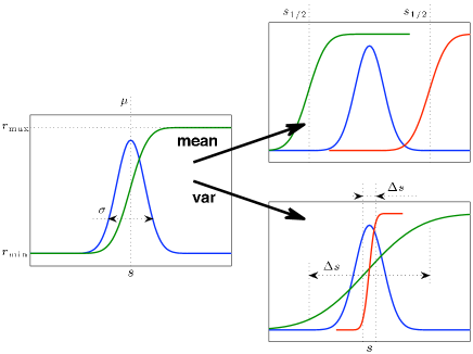
Figure 1: Parameters characterizing response to a signal. Left panel: the probability distribution of the signal, $P(s)$ (blue), and the best-matched steady state dose-response curve $r_{\rm ss}$ (green). Top right: if the mid-point of the dose-response curve, $s_{1/2}$, is far away from the mean of the signal, a typical response will be extremal. Bottom right: if the width of the dose-response curve, $\Delta s$, is considerably different from the standard deviation of the signal, then the typical response is either extremal, or at its mid-point. These mismatches prevent using the entire dynamic range of the response to convey information about the signal.

The distribution of stimuli, $P[s(t)]$, places severe constraints on admissible forms of $f$. To see this, for quasi-stationary signals (that is, when the signal correlation time $\tau$ is large, $\tau\gg 1/k$), we use Eq. (1) to write the steady state dose-response curve

$$r_{\rm ss}=f\left(s(t)\right)/k.$$ (2)

A typical monotonic, sigmoidal $f$ is characterized by only a few large-scale parameters: the range, $[f_{\min},f_{\max}]$; the mid-point $s_{1/2}$; and the width of the transition region, $\Delta s$ (cf. Fig. 1). If the signal mean $\mu\gg s_{1/2}$, then, for most signals, $r_{\rm ss}\approx f_{\rm max}/k$. Then responses to two different signals $s_{1}$ and $s_{2}$ are indistinguishable as long as

$$\left.\frac{dr_{\rm ss}(s)}{ds}\right|_{s=s_{1}}(s_{2}-s_{1})<\delta r,$$ (3)

where $\delta r$ is the precision of the response resolution. Similarly, when $\mu\ll s_{1/2}$, then $r_{\rm ss}\approx f_{\rm min}/k$. Thus, for reliably communicating information about the signal, $f$ should be tuned such that $s_{1/2}\approx\mu$. If a biological system can change its $s_{1/2}$ to follow changes in $\mu$, this is called adapting to the mean of the signal, and, if $s_{1/2}(\mu)=\mu$, then the adaptation is perfect [1, 2]. Similarly, if the quasi-stationary signal is taken from the distribution with $\sigma\equiv\left(\langle s(t)^{2}\rangle_{t}-\mu^{2}\right)^{1/2}\gg\Delta s$, then the response to most of the signals will be indistinguishable from the extrema. It will be near $\sim(r_{\max}+r_{\min})/2$ if $\sigma\ll\Delta s$. Thus, to use the full dynamic range of the response, a biological system must tune the width of the sigmoidal dose-response curve to $\Delta s\approx\sigma$; this is called the variance adaptation or gain control [2].

Both of these adaptation behaviors can be traced to the same theoretical argument [3]: for sufficiently general conditions on the response resolution $\delta r$, the response that optimizes the fidelity of a signaling system, as measured by its information-theoretic channel capacity [4], is $r_{\rm ss}^{*}(s)=\int_{-\infty}^{s}P(s^{\prime})ds^{\prime}$, where $P(s^{\prime})$ is the probability distribution of an instantaneous signal value, obtained from $P[s(t)]$. However, since environmental changes that lead to varying $\mu$ and $\sigma$, as well as mechanisms of the adaptation may be distinct, it often makes sense to consider the two adaptations as separate phenomena [2].

Adaptation to the mean, sometimes also called desensitization, has been observed and studied in a wide variety of biological sensory systems [1, 5, 3, 6, 7], with active work persisting to date. In contrast, while gain control has been investigated in neurobiology [8, 9, 10], we are not aware of its systematic analysis in molecular sensing. In this article, we start filling in the gap. Our main contribution is the observation that a mechanism for gain control, observed in a fly motion estimation system by Borst et al. [10], can be transferred to molecular information processing with minimal modifications. Importantly, unlike adaptation to the mean, which is implemented typically using extra feedback circuitry [1, 7, 11], the gain control mechanism we analyse requires no additional regulation. It is built-in into many molecular signaling systems. The main ingredients of the gain control mechanism in Ref. [10] is a strongly nonlinear, sigmoidal response function $f(s)$ and a realization that real-world signals are dynamic with a nontrivial temporal structure. Thus one must move away from the steady state response analysis and autocorrelations within the signals will allow the response to carry more information about the signal than seems possible naively.

Specifically, we show that even a simple biochemical circuit in Eq. (1), with no extra regulatory features can be made insensitive to changes in $\sigma$. That is, for an arbitrary choice of $\sigma$, and for a wide range of other parameters, the circuit can generate an output that is informative of the input, and, in particular, carries more than a single bit of information about it. For brevity, we will not review the original work on gain control in neural systems [10], but will instead develop the methodology directly in the molecular context.

2 Results: Gain control with no additional regulatory structures

Let’s assume for simplicity that the signal in Eq. (1) has the Ornstein-Uhlenbeck dynamics with:

$$\langle s(t)\rangle=\mu,\;\;\langle s(t+t^{\prime})s(t)\rangle=\sigma^{2}e^{-t^{\prime}/\tau}.$$ (4)

We will assume that the response has been adapted to the mean value of this signal (likely by additional feedback control circuitry, not considered here explicitly), so that the response to $s=\mu$ is half maximal. Now we explore how insensitivity to $\sigma$ can be achieved as well.

We start with a step-function approximation to the sigmoidal response synthesis

$$f=f_{0}\theta(s-\mu)=f_{0}\times\left\{\begin{array}[]{l}0,\;s<\mu,\\ 1/2,\;s=\mu^{\prime},\\ 1,\;s>\mu,\end{array}\right.$$ (5)

where $f_{0}$ is some constant. This is a limiting case of very high Hill number dose-response curves, which have been observed in nature [12]. Figure 2 shows sample signals and responses produced by this system. Notice that such $f$ makes the system manifestly insensitive to $\sigma$. Any changes in $\sigma$ will not result in changes to the response, hence the gain is controlled perfectly.

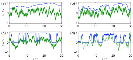
Figure 2: Examples of signals and responses for dynamics in Eqs. (1, 4, 5). On the vertical axis, we plot normalized signals $s_{s}=(s-m)/\max(s)$ (green) and normalized responses $r=r/\max(r)$ (blue). On the horizontal axis, the time is rescaled by the correlation time of the signal, $\tau$. Panels (a)-(c) have $k\tau=0.1,1,10$, respectively [recall that $1/k$ is the response time of the circuit, Eq. (1)]. In panel (d), we show, for comparison, the firing rate of a blow fly motion sensitive neuron H1 and its driving stimulus, both rescaled to one (see [13] for details of this experiment). The stimulus had little power at high frequencies, but the single-exponential correlation structure held for long times. Notice the similarity between the telegraph-series-like structure of the responses in panels (c) and (d). Since the H1 neuron served as a model neural system for the feedback-free gain adaptation in [10], this similarity suggests to look for gain-controlled responses in molecular signaling, Eq. (1), as well.

Nevertheless, this choice of $f$ is pathological, resulting in a binary steady state response ($r_{\rm ss}=0$ for $s<\mu$, and $r_{\rm ss}=f_{0}/k$ otherwise). That is, the response cannot carry more than one bit of information about the stimulus. However, as illustrated in Fig. 2, a dynamic response is not binary and varies over its entire dynamic range. Can this make a difference and produce a dose-response relation that is both high fidelity and insensitive to the variance of the signal?

To answer this, we first specify what we mean by the dose-response curve or the input-output relation when there is no steady state response. For the response at a single time point $t$, we can write $P\left(r\left(t\right)|\{s\left(t^{\prime}\leq t\right)\}\right)=\delta(r-r[s])$, where $\delta(\cdots)$ is the Dirac $\delta$-function, and the functional $r[s]$ is obtained by solving Eq. (1). Since the signal is probabilistic, marginalizing over all but the instantaneous value of it at time $t-t^{\prime}$, one gets $P\left(r\left(t\right)|s\left(t-t^{\prime}\right)\right)$, the distribution of the response at time $t$ conditional on the value of the signal at $t-t^{\prime}$. Further, for the distribution of the signal given by Eq. (4), one can numerically integrate Eq. (1) and evaluate the correlation $c(t^{\prime})=\langle r(t)s(t-t^{\prime})\rangle_{t}$ . Since Eq. (1) is causal, $c(t^{\prime})$ has a maximum at some $t^{\prime}=\Delta(\tau,k)\geq 0$, illustrated in Fig. 3. Correspondingly, in this paper we replace the familiar notion of the dose-response curve by the probabilistic input-output relation $P(r(t)|s(t-\Delta))$.

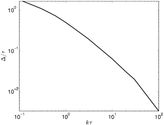
Figure 3: Dependence of the delay between the signal and the response, $\Delta$, which achieves the maximum correlation between $s$ and $r$. Here $\Delta$ is expressed in units of the signal correlation time $\tau$, and it is studied as a function of $k\tau$, the ratio of characteristic time scales of the signal and the response dynamics.

In Fig. 4, we plot the input-output relation for $k\tau=10$. To emphasize the independence of the response on $\sigma$ and hence the gain-compensating nature of the system, we plot $s$ in units of $\sigma$. A smooth, probabilistic, sigmoidal response with a width of the transition region $\Delta\sim\sigma$ is clearly visible. This is because, for a step-function $f$, the value of $r(t)$ depends not on $s(t)$, but on how long the signal has been positive prior to the current time. In its turn, this duration is correlated with $s/\sigma$, producing a probabilistic dependence between $r$ and $s/\sigma$. The latter is manifestly invariant to variance changes.

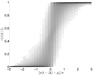
Figure 4: Conditional distribution $P(r(t)|s(t-\Delta))$ for $k\tau=10$. The signals are discretized into 30 values in the range of $[-3\sigma,+3\sigma]$. For each $s(t-\Delta)$, a histogram of $r(t)$ is built with 100 distinct $r$ values. The normalized histograms are grey-scale coded as columns on the plot, with dark representing the higher conditional probability, $P\sim 1$. We use a nonlinear color scale to enhance the plot.

These arguments make it clear that the fidelity of the response curve should depend on the ratio of characteristic times of the signal and the response, $k\tau$. Indeed, as seen in Fig. 2, for $k\tau\to 0$, the response integrates the signal over long times. It is little affected by the current value of the signal and does not span the full available dynamic range. At the other extreme of a very fast response, $k\tau\to\infty$, the system is almost quasi-stationary. Then the step-nature of $f$ is evident, and the response quickly swings between two limiting values ($f_{0}/k$ and 0).

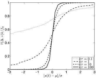
Figure 5: Mean conditional response $\bar{r}(\Delta,s)$ for different combinations of the signal and the response characteristic times, $k\tau$.

We illustrate the dependence of the response conditional distribution on the integration time in Fig. 5 by plotting $\bar{r}(\Delta,s)=\int dr\,r(t+\Delta)P(r(t+\Delta)|s(t))$, the conditional-averaged response for different values of $k\tau$. Neither $k\tau\to 0$ nor $k\tau\to\infty$ are optimal for signal transmission. One expects existence of an optimal $k^{*}$, for which most of the dynamic range of $r$ gets used, but the response is not completely binary. To find this optimum, we evaluate the mutual information [4] between the signal and the response at the optimal delay, $I_{k}[r(t+\Delta),s(t)]$, as a function of $k\tau$, cf. Fig. 6. A broad maximum in information transmission is observed near $k^{*}\approx 20/\tau$, which is not too far from the quasi-stationary limit. However, $I_{\max}\equiv I_{k^{*}}=1.37$ bits is substantially larger than 1. Thus temporal correlations in the stimulus allow to transmit 37% more information about it than the step response would suggest naively. This information is transmitted in a gain-controlled manner, so that changes in $\sigma$ have no effect. Similar conclusion should hold for non-step-like $f$, as long as $f$ is sigmoidal and $\Delta s/\sigma\ll 1$.

Figure 6: The signal-response mutual information at the optimal temporal delay as a function on $k\tau$. The solid line represents $I_{k}[r(t+\Delta),s(t)]$, the information for the Ornstein-Uhlenbeck signal, and the maximum of the information here is $I_{\max}=1.37$ bits, achieved at $k^{*}\approx 20/\tau$. The dashed line stands for the same information for the smoothed signal. It is maximized at $k^{*}\approx 3/\tau$ with $I_{\max}=1.35$ bits.

Effects of the signal structure. The observed gain insensitivity depends only weakly on details of the temporal structure of the signal. As long as there are autocorrelations, one can use them to transmit more than one bit about the signal in a gain-independent fashion using the strong nonlinearity of $f$. To verify this, we replace the Ornstein-Uhlenbeck signal, Eq. (4), with its low-pass filtered version, $s^{\prime}(t)=1/k\int^{t}dt^{\prime}s(t^{\prime})e^{-k(t-t^{\prime})}$, and $k$ is the same as in Eq. (1). This new signal is smoother and has less structure at high frequencies. We repeat the same analysis as above to find $\Delta$, estimate the conditional response distribution, and then evaluate $I_{k}$, the stimulus-response information. We find that the maximum information in this case is $I_{\max}=1.35$ bits, statistically indistinguishable from the Ornstein-Uhlenbeck case. However, the maximum is now at $k\tau\approx 3$. This is because the smooth signal has a lot fewer short-lived zero-crossings, and smaller integration times are needed to approach the extreme values of the response.

Knowing $\sigma$ in a gain-insensitive response. When gain-insensitive, the system looses information about the actual signal variance. This rarely happens in biology. For example, while we see well at different ambient light levels, we nonetheless know how bright it is outside. For the fly visual system, it was shown that variance independence of the response breaks on long time scales. The signal variance can be inferred from long-term features of the neural code [8, 14]. Correspondingly, we ask if long term observation of the response of an approximately gain-controlled molecular signaling circuit allows to infer the signal variance $\sigma$.

To this extent, consider $f$ as a narrow sigmoid, with the width of the crossover region $\Delta s/\sigma\ll 1$. The effect of the variance on the response is still negligible. For concreteness, we take $f=f_{0}[\tanh((s-\mu)/\Delta s)+1]$. Consider now the fraction of time the derivative of the response is near $\max(f)$. This requires that $r\approx 0$ (so that the degradation, $kr$, is negligible), but $s$ is already large, $(s-\mu)/\Delta s\gg 1$. The probability of this happening depends on the signal variance and hence on the speed with which the signal crosses over the threshold region. Thus one can estimate $\sigma$ by observing a molecular circuit for a long time and counting how often the rate of change of the response is large. While the probability of a large derivative will depend on the exact shape of $f$, for a signal defined by Eq. (4), the statistical error of any such counting estimator will scale as $\propto\sqrt{\tau/T}$. Hence, the system can be almost insensitive to $\sigma$ on short time scales, but allow its determination from long observations.

To verify this, we simulate the signal determined by Eq. (4) with the $k\tau=20$, which maximizes the signal-response mutual information. We calculate the mean fraction of time $\phi$ when the response derivative is above 80% of its maximum value. We further calculate the standard deviation of the fraction $\sigma_{\phi}$. We repeat this for signals with various $\Delta s/\sigma$ and for for experiments of different duration, obtaining a time-dependence of the $Z$-score for disambiguating two signals with different variances $Z=(\phi_{2}-\phi_{1})/\sqrt{\sigma_{\phi_{1}}^{2}+\sigma_{\phi_{2}}^{2}}$, where the indeces $1,2$ denote the signals being disambiguated. For example, for distinguishing signals with $\Delta s/\sigma=1/10$ and $1/20$, we estimate $Z\approx 0.8(T/\tau)^{0.48\pm 0.04}$, consistent with the square root scaling (the error bars indicate the 95% confidence interval). That is, for $T/\tau$ as little as 10, $Z>2$, and the two signals are distinguishable. Signals with larger variances are harder to disambiguate. For example, for $\Delta s/\sigma=1/90$ and $1/100$, $Z\approx 9.4\times 10^{-3}(T/\tau)^{0.56\pm 0.08}$, and $Z$ crosses 2 for $T\approx 15000\tau$.

This long-term variance determination can be performed molecularly in many different ways. For example, one can use a feedforward incoherent loop with $r$ as an input [15]. The loop acts as a approximate differentiator for signals that change slowly compared to its internal relaxation times [16]. The output species of the loop can then activate a subsequent species by a Hill-like dynamics, with the activation threshold close to the maximum of the possible derivative. If this last species degrades slowly, it will integrate the fraction of time when $dr/dt$ is above the threshold, providing the readout of the signal variance.

3 Discussion

In this article, we have argued that simple molecular circuitry can respond to signals in a gain-insensitive way without a need for adaptation and feedback loops. That is, these circuits can be sensitive only to the signal value relative to its standard deviation. To make the mechanism work, the signaling system must obey the following criteria

• a nonlinear-linear (NL) response; that is, a strongly nonlinear, sigmoidal synthesis function $f$ integrated (linearly) over time;

• properly matched time scales of the signal and the response dynamics.

In addition, the information about the signal variance can be recovered, for example, if

• large excursions of the response derivative can be counted over long times.

Naively transmitted information of only one bit (on or off) would be possible with a step-function synthesis $f$. However, the response in this system is a time-average of a nonlinear function of the signal. This allows to use temporal correlations in the signal to transmit more than 1 bit of information for broad classes of signals. While 1.35 bits may not seem like much more than 1, the question of whether biological systems can achieve more than 1 bit at all is still a topic of active research [17, 18]. Similar use of temporal correlations has been reported to increase information transmission in other circuits, such as clocks [19]. In practice, in our case, there is a tradeoff between variance-independence and high information transmission through the circuit: a wider synthesis function would produce higher maximal information for properly tuned signals, but the information would drop down to zero if $\Delta s\gg\sigma$. It would be interesting to explore the optimal operational point for this tradeoff under various optimization hypotheses.

While our analysis is applicable to any molecular system that satisfies the three conditions listed above, there are specific examples where we believe it may be especially relevant. The E. coli chemotaxis flagellar motor has a very sharp response curve (Hill coefficient of about 10) [12]. This system is possibly the best studied example of biological adaptation to the mean of the signal. However, the question of whether the system is insensitive to the signal variance changes has not been addressed. The ultrasensitivity of the motor suggests that it might be. Similarly, in eukaryotic signaling, push-pull enzymatic amplifiers, including MAP kinase mediated signaling pathways, are also known for their ultrasensitivity [20, 21, 22]. And yet ability of these circuits to respond to temporally-varying signals in a variance-independent way has not been explored.

We end this article with a simple observation. While the number of biological information processing systems is astonishing, the types of computations they perform are limited. Focusing on the computation would allow cross-fertilization between seemingly disparate fields of quantitative biology. The phenomenon studied here, lifted wholesale from neurobiology literature, is an example. Arguably, computational neuroscience has had a head start compared to computational molecular systems biology. The latter can benefit immensely by embracing well-developed results and concepts from the former.

References

References

- [1] H Berg. E. coli in motion. Springer-Verlag, New York, 2003.
- [2] I Nemenman. Information theory and adaptation. In M Wall, editor, Quantitative biology: From molecules to Cellular Systems. CRC Press, In press.
- [3] S Laughlin. A simple coding procedure enhances a neuron’s information capacity. Z Naturforsch, 36:910, 1981.
- [4] C Shannon and W Weaver. The mathematical theory of communication. The University of Illinois Press, Urbana, IL, 1949.
- [5] R Normann and I Perlman. The effects of background illumination on the photoresponses of red and green cells. J Physiol, 286:491, 1979.
- [6] D MacGlashan, S Lavens-Phillips, and M Katsushi. IgE-mediated desensitization in human basophils and mast cells. Front Biosci, 3:746–56, 1998.
- [7] P Detwiler, S Ramanathan, A Sengupta, and B Shraiman. Engineering aspects of enzymatic signal transduction: Photoreceptors in the retina. Biophys J, 79:2801, 2000.
- [8] N Brenner, W Bialek, and R de Ruyter van Steveninck. Adaptive rescaling optimizes information transmission. Neuron, 26:695, 2000.
- [9] K Gaudry and P Reinagel. Contrast adaptation in a nonadapting lgn model. J Neurophysiol, 98:1287–96, 2007.
- [10] A Borst, V Flanagin, and H Sompolinsky. Adaptation without parameter change: Dynamic gain control in motion detection. Proc Natl Acad Sci USA, 102:6172, 2005.
- [11] W Ma, A Trusina, H El Samad, W Lim, and C Tang. Defining network topologies that can achieve biochemical adaptation. Cell, 138:760–73, 2009.
- [12] P Cluzel, M Surette, and S Leibler. An ultrasensitive bacterial motor revealed by monitoring signaling proteins in single cells. Science, 287:1652, 2000.
- [13] I Nemenman, G Lewen, W Bialek, and R de Ruyter van Steveninck. Neural coding of natural stimuli: Information at sub-millisecond resolution. PLoS Comput Biol, page e1000025, 2008.
- [14] A Fairhall, G Lewen, W Bialek, and R de Ruyter van Steveninck. Efficiency and ambiguity in an adaptive neural code. Nature, 412:787, 2001.
- [15] S Mangan and U Alon. Structure and function of the feed-forward loop network motif. Proc Natl Acad Sci USA, 100:11980–5, 2003.
- [16] E Sontag. Remarks on feedforward circuits, adaptation, and pulse memory. IET Syst Biol, 4:39–51, 2010.
- [17] E Ziv, I Nemenman, and C Wiggins. Optimal signal processing in small stochastic biochemical networks. PLoS One, 2:e1077, 2007.
- [18] G Tkacik, C Callan, and W Bialek. Information capacity of genetic regulatory elements. Phys Rev E, 78:011910, 2008.
- [19] A Mugler, A Walczak, and C Wiggins. Information-optimal transcriptional response to oscillatory driving. Phys Rev Lett, 105:058101, 2010.
- [20] A Goldbeter and D Koshland. An amplified sensitivity arising from covalent modification in biological systems. Proc Natl Acad Sci USA, 78:6840–4, 1981.
- [21] C Huang and J Ferrell. Ultrasensitivity in the mitogen-activated protein kinase cascade. Proc Natl Acad Sci USA, 93:10078–83, 1996.
- [22] M Samoilov, S Plyasunov, and A Arkin. Stochastic amplification and signaling in enzymatic futile cycles through noise-induced bistability with oscillations. Proc Natl Acad Sci USA, 102:2310–5, 2005.