Velocity correlations of a discrete-time totally asymmetric simple-exclusion process in stationary state on a circle

Abstract

The discrete-time version of totally asymmetric simple-exclusion process (TASEP) on a finite one-dimensional lattice is studied with the periodic boundary condition. Each particle at a site hops to the next site with probability $0\leq p\leq 1$, if the next site is empty. This condition can be rephrased by the condition that the number $n$ of vacant sites between the particle and the next particle is positive. Then the average velocity is given by a product of the hopping probability $p$ and the probability that $n\geq 1$. By mapping the TASEP to another driven diffusive system called the zero-range process, it is proved that the distribution function of vacant sites in the stationary state is exactly given by a factorized form. We define $k$-particle velocity correlation function as the expectation value of a product of velocities of $k$ particles in the stationary distribution. It is shown that it does not depend on positions of $k$ particles on a circle but depends only on the number $k$. We give explicit expressions for all velocity correlation functions using the Gauss hypergeometric functions. Covariance of velocities of two particles is studied in detail and we show that velocities become independent asymptotically in the thermodynamic limit.

I Introduction

The one-dimensional totally asymmetric simple-exclusion process (TASEP) is a minimal statistical-mechanics model for driven diffusive systems of many particles with hardcore exclusive interaction Lig85 ; Spo91 ; SZ95 ; Lig99 ; Sch00 ; MKL09 . In the present paper, we consider a discrete-time version of the TASEP on a circle, i.e. a one-dimensional finite lattice with periodic boundary condition, in which the parallel update rule is applied RSSS98 . This process can be exactly mapped to another driven diffusive particle system called the zero-range process (ZRP), by regarding each number of vacant sites between successive particles in the TASEP as a number of particles at each site in the ZRP Eva00 ; EH05 .

In the ZRP representation, particles hop from site to site on a lattice with a hopping probability which depends only on the number of particles at the departure site. We assume that there do not occur any creation and annihilation of particles in the ZRP. Then, if a site is vacant, there is no possibility that a particle hops from that empty site to other sites, as a matter of course. The configuration in the TASEP such that the next site of a particle is occupied by another particle is represented by the configuration in the ZRP such that the corresponding site is empty. Therefore the prohibition of hopping by hardcore exclusion in such a jamming situation in the TASEP is automatically satisfied in the ZRP. Moreover, the steady state of the ZRP is exactly described by the probability density function in a factorized form Eva00 ; EH05 , and then the stationary distribution of vacant sites in the TASEP on a circle is explicitly determined as Eq.(5) given below Eva00 ; EH05 ; KNT06 ; Kan07 .

The map from the TASEP to the ZRP is interesting from the viewpoint of quantum statistical mechanics, since it seems to be a map from an interacting Fermi gas to a free Bose gas. On the other hand, as demonstrated in the present paper, the procedure in which we analyze the TASEP/ZRP is quite different from the standard way for free Boson systems in the following sense. (i) Thermal equilibrium state of free Bose gas is usually treated in the grand canonical ensemble by introducing fugacity, while here we want to consider the driven diffusive system with a fixed number of particles and thus we treat the system in the canonical ensemble. Then the canonical partition function $Z_{L,N}$, where $L$ and $N$ denote the numbers of particles and vacancies in the TASEP, respectively, plays an important role in calculation. (ii) In the usual theory of free Bose gases, condensation of particles in a specified energy level is carefully studied (e.g., the Bose-Einstein condensation in a ground state). In the context of ZRP, however, distribution of vacancies (i.e., empty energy levels) should be well studied. The reason is that, if a site in the ZRP is occupied by one or more than one particle, then the velocity of the corresponding particle in the TASEP can be positive, but if the site is empty in the ZRP, the velocity of the particle in the TASEP is definitely zero. When we consider the TASEP as a simple model of traffic flow, the flux which is defined as the product of velocity and particle-density is the most important quantity. The purpose of the present paper is to study velocity correlations of particles in the stationary state of the TASEP on a circle.

Let ${\bf N}=\{1,2,3,\dots\}$ and ${\bf N}_{0}=\{0\}\cup{\bf N}=\{0,1,2,\dots\}$. For $K\in{\bf N}$, we consider a one-dimensional lattice $\Lambda=\{1,2,\dots,K\}$. Each site $i\in\Lambda$ is either occupied by a particle, which is denoted by $\eta(i)=1$, or vacant denoted by $\eta(i)=0$. The following discrete-time stochastic process is considered for simulating the TASEP on a circle. Let $0\leq p\leq 1$. At each time $t\in{\bf N}_{0}$, given a particle configuration $\eta_{t}=\{\eta_{t}(i)\}_{i\in\Lambda}\in\{0,1\}^{\Lambda}$, let $A_{t}=\{(i,i+1):1\leq i\leq K,\,\mbox{s.t.}\,\eta_{t}(i)=1,\eta_{t}(i+1)=0\}$, where the periodicity $\eta(i+K)=\eta(i),i\in\Lambda$ is assumed and the nearest-neighbor pair of sites $(K,K+1)$ is identified with $(K,1)$. Every particle at site $i$ such that $(i,i+1)\in A_{t}$ has chance to move to its next site $i+1$, since the site $i+1$ is vacant; $\eta_{t}(i+1)=0$. But, in general, only a part of such particles move depending on the parameter $p$ as follows. We choose a subset of $A_{t}$ randomly, in the sense that each pair of nearest-neighbor sites $(i,i+1)\in A_{t}$ is chosen independently with probability $p$. The obtained subset of $A_{t}$ is written as $\widehat{A_{t}}$. In the present paper, the total number of elements included in a set $B$ is denoted by $|B|$ and, for $B\subset C$, the complementary set of $B$ in the set $C$ is expressed by $C\setminus B$. (By definition $|C\setminus B|=|C|-|B|$.) Then the probability that $\widehat{A_{t}}$ is chosen from $A_{t}$ is given by $p^{|\widehat{A_{t}}|}(1-p)^{|A_{t}|-|\widehat{A_{t}}|}$. Only the particles at sites $\{i\}$ such that $(i,i+1)\in\widehat{A_{t}}$ indeed move to their next sites. That is, the particle configuration at time $t+1$, $\eta_{t+1}=\{\eta_{t+1}(i)\}_{i\in\Lambda}$, is given by

$$\eta_{t+1}(i)=\left\{\begin{array}[]{ll}\eta_{t}(i)-1,&\quad\mbox{if $(i,i+1)\in\widehat{A_{t}}$},\\ \eta_{t}(i)+1,&\quad\mbox{if $(i-1,i)\in\widehat{A_{t}}$},\\ \eta_{t}(i),&\quad\mbox{otherwise}.\end{array}\right.$$ (1)

Here note that by definition of $\widehat{A_{t}}$, if $(i,i+1)\in\widehat{A_{t}}$, then $(i-1,i)\notin\widehat{A_{t}}$. The parameter $p$ is called the hopping probability and the above procedure is said to be the parallel update rule. The total number of particles is conserved in the process, which we write $L$ in the present paper. We assume $1\leq L\leq K$.

Given a particle configuration $\eta\in\{0,1\}^{\Lambda}$, let $i_{1}=\min\{1\leq i\leq K:\eta(i)=1\}$ and define

$$i_{j+1}=\min\{i_{j}<i\leq K:\eta(i)=1\},\quad 1\leq j\leq L-1,$$ (2)

i.e., $i_{j}$ is the site occupied by the $j$-th particle, $1\leq j\leq L$. Then we put

$$n(j)=i_{j+1}-i_{j}-1,\quad 1\leq j\leq L,$$ (3)

where $i_{L+1}\equiv i_{1}+K$. That is, $n(j)$ gives the number of vacant sites between the $j$-th and the $(j+1)$-th particles. By (3) with (2), a configuration of vacancies ${\bf n}=\{n(j)\}_{j=1}^{L}$ is uniquely determined from the particle configuration $\eta=\{\eta(i)\}_{i=1}^{K}$.

We should note that ${\bf n}$ does not determine $\eta$ uniquely, however, since the information on the position of the first particle, $i_{1}$, is missing in the map $\eta\to{\bf n}$. This information may be, however, not important, since here we consider the TASEP on a circle. The stochastic process ${\bf n}_{t}=\{n_{t}(j)\}_{j=1}^{L},t\in{\bf N}_{0}$, obtained from $\eta_{t},t\in{\bf N}_{0}$ by this map, is a special case of the ZRP Eva00 ; EH05 . As a consequence of general theory of ZRP Eva97 ; EH05 ; KNT06 ; Kan07 , the probability distribution function in the stationary state ${\bf P}_{L,N}({\bf n})$ of configuration ${\bf n}$ of vacancies is uniquely determined as follows. Since the lattice size $K$ and the total number of particles $L$ are conserved, the total number of vacant sites $N\equiv\sum_{j=1}^{L}n(j)=K-L$ is also a constant. We fix $1\leq L,N\leq K$. Then the configuration space of ${\bf n}$ is given by

$$\Omega_{L,N}=\left\{{\bf n}=\{n(j)\}_{j=1}^{L}\in\{0,1,\dots,N\}^{L}:\sum_{j=1}^{L}n(j)=N\right\}$$ (4)

and

$${\bf P}_{L,N}({\bf n})=\frac{1}{Z_{L,N}}\prod_{j=1}^{L}f(n(j)),\quad{\bf n}=\{n(j)\}_{j=1}^{L}\in\Omega_{L,N},$$ (5)

where Remark1

$$f(n)=\left\{\begin{array}[]{ll}1,&\quad\mbox{if $n=0$},\\ (1-p)^{n-1},&\quad\mbox{if $n\geq 1$},\end{array}\right.$$ (6)

and the partition function is given by KNT06 ; Kan07 .

$$Z_{L,N} \equiv \sum_{{\bf n}\in\Omega_{L,N}}\prod_{j=1}^{L}f(n(j))$$ (7)

$$= (1-p)^{N-1}LF\left(1-L,1-N;2;\frac{1}{1-p}\right)$$

$$= \frac{(-p)^{L+N}L}{(1-p)^{L+1}}F\left(L+1,N+1;2;\frac{1}{1-p}\right)$$

with the Gauss hypergeometric function AS72

$$F(\alpha,\beta;\gamma;z)=\sum_{n=0}^{\infty}\frac{(\alpha)_{n}(\beta)_{n}}{(\gamma)_{n}}\frac{z^{n}}{n!},$$ (8)

$(\alpha)_{0}=1,(\alpha)_{n}=\alpha(\alpha+1)\cdots(\alpha+n-1),n\geq 1$. Note that the last equality in (7) is due to Kummer’s transformation AS72

$$F(\alpha,\beta;\gamma;z)=(1-z)^{\gamma-\alpha-\beta}F(\gamma-\alpha,\gamma-\beta;\gamma;z).$$

We write the expectation with respect to the stationary distribution (5) as ${\bf E}_{L,N}[\,\cdot\,]$ in this paper.

For the $j$-th particle, $1\leq j\leq L$, if $n(j)\geq 1$, that is, if $n(j)\not=0$, then that particle can move to the next site with probability $p$ in a time-step. Then if the velocity of $j$-th particle is denoted by $V_{j}$, the expectation of this random variable in the stationary distribution ${\bf P}_{L,N}$ is given by

$${\bf E}_{L,N}[V_{j}] = p{\bf E}_{L,N}[{\bf 1}(n(j)\geq 1)]$$ (9)

$$= p\sum_{{\bf n}\in\Omega_{L,N}}{\bf 1}(n(j)\geq 1){\bf P}_{L,N}({\bf n}),$$

where ${\bf 1}(\omega)$ is an indicator of an event $\omega$; ${\bf 1}(\omega)=1$ if $\omega$ occurs, ${\bf 1}(\omega)=0$ otherwise. The average velocity (9) is independent of $j$, since the system is homogeneous in space, and it has been explicitly calculated as KNT06 ; Kan07

$${\bf E}_{L,N}[V] = \frac{\sum_{n=0}^{N-1}(-1)^{N+1-n}Z_{L,n}}{Z_{L,N}}$$ (10)

$$= \frac{p}{L}\frac{F(1-L,1-N;1;1/(1-p))}{F(1-L,1-N;2;1/(1-p))}$$

$$= -\frac{1-p}{L}\frac{F(L,N;1;1/(1-p))}{F(L+1,N+1;2;1/(1-p))}.$$

The density of particles is given by

$$\rho=\frac{L}{L+N}=\frac{L}{K},$$ (11)

and the flux $J_{L,N}$ is defined by

$$J_{L,N}=\rho{\bf E}_{L,N}[V].$$ (12)

If we plot $J_{L,N}$ versus $\rho$, we obtain a fundamental diagram as demonstrated by Kanai Kan07 (see Fig.1 in the present paper). Moreover, Kanai et al.KNT06 determined the thermodynamic limit, i.e. the scaling limit of $L\to\infty,N\to\infty$ with keeping $\rho=L/(L+N)$ be a constant, for the average velocity and obtained (see Fig.1)

$$\lim_{\begin{subarray}{c}L\to\infty,N\to\infty;\\ \rho={\rm const.}\end{subarray}}{\bf E}_{L,N}[V]=\frac{1-\sqrt{1-4p\rho(1-\rho)}}{2\rho},\quad 0\leq\rho,p\leq 1.$$ (13)

This result coincides with the exact solution for an infinite system obtained by Schadschneider and Schreckenberg SS93 .

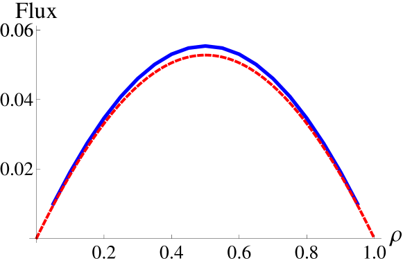
Figure 1: The fundamental diagrams. The flux $J_{L,N}$ is plotted versus $\rho$ for $K=20$ with $p=0.2$ by a solid line. The broken line shows the thermodynamic limit (13) with $p=0.2$. We find that the difference between the results for finite systems and the thermodynamic limit is very small, in particular, when $\rho\simeq 0$, $\rho\simeq 1.0$.

In the present paper, we study velocity correlation functions and show that, as extensions of the formula (10), they are generally expressed by using the Gauss hypergeometric functions. In particular, the covariance of velocities $V$ and $V^{\prime}$ of two particles at different sites,

$${\rm Cov}_{L,N}[V,V^{\prime}]={\bf E}_{L,N}[VV^{\prime}]-{\bf E}_{L,N}[V]^{2},$$ (14)

is studied in detail and it is shown that

$$\lim_{\begin{subarray}{c}L\to\infty,N\to\infty;\\ \rho={\rm const.}\end{subarray}}{\rm Cov}_{L,N}[V,V^{\prime}]=0.$$ (15)

That is, velocities of particles are correlated in the stationary state in any finite systems, but it is proved that they become independent asymptotically in the thermodynamic limit in the discrete-time TASEP on a circle.

The paper is organized as follows. In Sec.II.A velocity correlation functions are defined and the general formula is derived. As special cases, the obtained expressions of average velocity and covariance of velocities of two particles are studied in detail in Sec.II.B and C, respectively. Sec.III is devoted to proving asymptotic independence of velocities (15) in the thermodynamic limit. Concluding remarks are given in Sec.IV. Appendix A is given for showing the derivation of a Riccati equation, which governs the covariance of velocities and is used in the proof in Sec.III.

II Velocity Correlation Functions

II.1 General Formula

Let $1\leq k\leq L$. From the $L$ particles, we pick up $k$ distinct particles arbitrarily; let $1\leq j_{1}<j_{2}<\cdots<j_{k}\leq L$, and consider a set of $k$ particles such that the $\ell$-th particle in this set, $1\leq\ell\leq k$, is originally the $j_{\ell}$-th particle in the whole particle systems. Write the velocity of the $j_{\ell}$-th particle by $V_{j_{\ell}},1\leq\ell\leq k$. The velocity correlation function for the $k$ particle is then defined by

$$F_{L,N}(\{V_{j_{\ell}}\}_{\ell=1}^{k}) = {\bf E}_{L,N}\left[\prod_{\ell=1}^{k}V_{j_{\ell}}\right]$$ (16)

$$= p^{k}\sum_{{\bf n}\in\Omega_{L,N}}\prod_{\ell=1}^{k}{\bf 1}(n(j_{\ell})\geq 1){\bf P}_{L,N}({\bf n}).$$

Since the stationary distribution function is given by the factorized form (5), it is written as

$$F_{L,N}(\{V_{j_{\ell}}\}_{\ell=1}^{k})=\frac{p^{k}}{Z_{L,N}}\sum_{n(1)=0}^{N}\sum_{n(2)=0}^{N}\cdots\sum_{n(L)=0}^{N}\prod_{\ell=1}^{k}{\bf 1}(n(j_{\ell})\geq 1)\prod_{j=1}^{L}f(n(j)){\bf 1}\left(\sum_{j=1}^{L}n(j)=N\right)$$

$$\quad=\frac{p^{k}}{Z_{L,N}}\prod_{j\in{\bf I}_{L}\setminus{\bf J}_{k}}\sum_{n(j)=0}^{N}f(n(j))\prod_{\ell\in{\bf J}_{k}}\sum_{n(\ell)=1}^{N}f(n(\ell)){\bf 1}\left(\sum_{i=1}^{L}n(i)=N\right)$$

$$\quad=\frac{p^{k}}{Z_{L,N}}\prod_{j\in{\bf I}_{L}\setminus{\bf J}_{k}}\sum_{n(j)=0}^{N}f(n(j))\prod_{\ell\in{\bf J}_{k}}\left(\sum_{n(\ell)=0}^{N}f(n(\ell))-f(0)\right){\bf 1}\left(\sum_{i=1}^{L}n(i)=N\right),$$ (17)

where ${\bf I}_{L}=\{1,2,\dots,L\}$ and ${\bf J}_{k}=\{j_{1},j_{2},\dots,j_{k}\}$.

We perform the binomial expansion

$$\prod_{\ell\in{\bf J}_{k}}\left(\sum_{n(\ell)=0}^{N}f(n(\ell))-f(0)\right)=\sum_{{\bf K}\subset{\bf J}_{k}}(-f(0))^{|{\bf J}_{k}\setminus{\bf K}|}\prod_{\ell\in{\bf K}}\sum_{n(\ell)=0}^{N}f(n(\ell)),$$ (18)

where the first summation in the RHS is taken over all subsets ${\bf K}$ of ${\bf J}_{k}$ and $|{\bf J}_{k}\setminus{\bf K}|$ is the number of elements in the complementary set of ${\bf K}$ in ${\bf J}_{k}$. Note that ${\bf I}_{L}=({\bf I}_{L}\setminus{\bf J}_{k})\cup{\bf K}\cup({\bf J}_{k}\setminus{\bf K})$ and $i\in{\bf J}_{k}\setminus{\bf K}$ implies $n(i)=0$, since the weight $f(0)/Z_{L,N}$ is assigned in the expansion. Therefore we can set $\sum_{i=1}^{L}n(i)=\sum_{i\in({\bf I}_{L}\setminus{\bf J}_{k})\cup{\bf K}}n(i)$ in (17). Since we set $f(0)=1$ as (6), we obtain

$$F_{L,N}(\{V_{j_{\ell}}\}_{\ell=1}^{k})$$

$$=\frac{p^{k}}{Z_{L,N}}\sum_{{\bf K}\in{\bf J}_{k}}(-1)^{|{\bf J}_{k}\setminus{\bf K}|}\prod_{j\in{\bf I}_{L}\setminus{\bf J}_{k}}\sum_{n(j)=0}^{N}f(n(j))\prod_{\ell\in{\bf K}}\sum_{n(\ell)=0}^{N}f(n(\ell)){\bf 1}\left(\sum_{i\in({\bf I}_{L}\setminus{\bf J}_{k})\cup{\bf K}}n(i)=N\right)$$

$$=\frac{p^{k}}{Z_{L,N}}\sum_{{\bf K}\in{\bf J}_{k}}(-1)^{|{\bf J}_{k}\setminus{\bf K}|}\prod_{i\in({\bf I}_{L}\setminus{\bf J}_{k})\cup{\bf K}}\sum_{n(i)=0}^{N}f(n(i)){\bf 1}\left(\sum_{i\in({\bf I}_{L}\setminus{\bf J}_{k})\cup{\bf K}}n(i)=N\right).$$ (19)

When $|{\bf J}_{k}\setminus{\bf K}|=s,0\leq s\leq k$, $|{\bf K}|=k-s$ and thus $|({\bf I}_{L}\setminus{\bf J}_{k})\cup{\bf K}|=|{\bf I}_{L}\setminus{\bf J}_{k}|+|{\bf K}|=(L-k)+(k-s)=L-s$. Therefore

$$\prod_{i\in({\bf I}_{L}\setminus{\bf J}_{k})\cup{\bf K}}\sum_{n(i)=0}^{N}f(n(i)){\bf 1}\left(\sum_{i\in({\bf I}_{L}\setminus{\bf J}_{k})\cup{\bf K})}n(i)=N\right)$$

$$\quad=\prod_{p=1}^{L-s}\sum_{n(p)=0}^{N}f(n(p)){\bf 1}\left(\sum_{p=1}^{L-s}n(p)=N\right)$$

$$\quad=\sum_{{\bf n}\in\Omega_{L-s,N}}\prod_{p=1}^{L-s}f(n(p))=Z_{L-s,N}.$$

Since the number of distinct subsets ${\bf K}$ in ${\bf J}_{k}$ satisfying $|{\bf J}_{k}\setminus{\bf K}|=s$ is $\displaystyle{{k\choose s}},0\leq s\leq k$, (19) is equal to $\{p^{k}/Z_{L,N}\}\sum_{s=0}^{k}(-1)^{s}{k\choose s}Z_{L-s,N}$. The result does not depend on the choice of particle positions ${\bf J}_{k}=\{j_{1},j_{2},\dots,j_{k}\}$, but depends only on the total number $k$ of particles, whose velocity correlation is calculated. This special property comes from the factorized form (5) of the stationary distribution in the present system, in which the factor $f(n)$ are independent of the system sizes, $L$ and $N$, as given by (6). We summarize the result by the following formula,

$$F_{L,N}(k) \equiv F_{L,N}(\{V_{j_{\ell}}\}_{\ell=1}^{k})$$ (20)

$$= \frac{p^{k}}{Z_{L,N}}\sum_{s=0}^{k}(-1)^{s}{k\choose s}Z_{L-s,N}$$

$$= \frac{p^{k}}{LF(1-L,1-N;2;1/(1-p))}$$

$$\quad\times\sum_{s=0}^{k}(-1)^{s}(L-s){k\choose s}F\left(1-L+s,1-N;2;\frac{1}{1-p}\right)$$

$$= \frac{p^{k}}{LF(L+1,N+1;2;1/(1-p))}$$

$$\quad\times\sum_{s=0}^{k}(L-s){k\choose s}\left(\frac{1-p}{p}\right)^{s}F\left(L-s+1,N+1;2;\frac{1}{1-p}\right).$$

It should be noted that still velocities are correlated in the sense that $F_{L,N}(k)\not=(F_{L,N}(1))^{k},k\geq 2$. In other words,

$${\bf E}_{L,N}\left[\prod_{\ell=1}^{k}V_{j_{\ell}}\right]\not=\prod_{\ell=1}^{k}{\bf E}_{L,N}\left[V_{j_{\ell}}\right],\quad k\geq 2.$$

II.2 Average Velocity

By setting $k=1$ in the general formula (20), we obtain

$${\bf E}_{L,N}[V]=F_{L,N}(1)=\frac{p}{Z_{L,N}}(Z_{L,N}-Z_{L-1,N})$$

$$=p\frac{LF(1-L,1-N;2;1/(1-p))-(L-1)F(2-L,1-N;2;1/(1-p))}{LF(1-L,1-N;2;1/(1-p))}$$

$$=\frac{LpF(L+1,N+1;2;1/(1-p))+(L-1)(1-p)F(L,N+1;2;1/(1-p))}{LF(L+1,N+1;2;1/(1-p))}.$$ (21)

Now we show that the last expression of (21) is equal to the last expression of (10). First we rewrite the numerator of (21) as

$$-(1-p)\Bigg{[}LF\left(L+1,N+1;2;\frac{1}{1-p}\right)-\frac{L}{1-p}F\left(L+1,N+1;2;\frac{1}{1-p}\right)$$

$$\qquad\qquad-(L-1)F\left(L,N+1;2;\frac{1}{1-p}\right)\Bigg{]}.$$ (22)

If we use the recurrence relation of the Gauss hypergeometric series AS72

$$\alpha zF(\alpha+1,\beta+1;\gamma+1;z)=\gamma\Big{\{}F(\alpha,\beta+1;\gamma;z)-F(\alpha,\beta;\gamma;z)\Big{\}}$$

for the second term in (22), (22) becomes

$$-(1-p)\Bigg{[}LF\left(L+1,N+1;2;\frac{1}{1-p}\right)-F\left(L,N+1;1;\frac{1}{1-p}\right)$$

$$\qquad\qquad+F\left(L,N;1;\frac{1}{1-p}\right)-(L-1)F\left(L,N+1;2;\frac{1}{1-p}\right)\Bigg{]}.$$ (23)

Next we apply the formula AS72

$$(\gamma-\alpha-1)F(\alpha,\beta;\gamma;z)+\alpha F(\alpha+1,\beta;\gamma;z)=(\gamma-1)F(\alpha,\beta;\gamma-1;z)$$

to the first and the fourth terms in (23). Then the sum of them becomes

$$LF\left(L+1,N+1;2;\frac{1}{1-p}\right)-(L-1)F\left(L,N+1;2;\frac{1}{1-p}\right)=F\left(L,N+1;1;\frac{1}{1-p}\right),$$

which is cancelled by the second term in (23). Therefore, the numerator of (21) is equal to $-(1-p)F(L,N;1;1/(1-p))$, and the equivalence of the last expression of (21) and the last expression of (10) is confirmed.

II.3 Covariance of Velocity

By the first expression in (20) for $k=2$, we obtain

$${\bf E}_{L,N}[VV^{\prime}] = F_{L,N}(2)$$ (24)

$$= \frac{p^{2}}{Z_{L,N}}(Z_{L,N}-2Z_{L-1,N}+Z_{L-2,N}).$$

Then the covariance of velocities (14) is given by

$${\rm Cov}_{L,N}[V,V^{\prime}]=p^{2}\left\{\frac{Z_{L-2,N}}{Z_{L,N}}-\left(\frac{Z_{L-1,N}}{Z_{L,N}}\right)^{2}\right\}.$$ (25)

By the expression of partition function (7) using the hypergeometric function, it is written as

$${\rm Cov}_{L,N}[V,V^{\prime}] = p^{2}\left\{\frac{(L-2)F(3-L,1-N;2;1/(1-p))}{LF(1-L,1-N;2;1/(1-p))}\right.$$ (26)

$$\qquad\qquad\left.-\left(\frac{(L-1)F(2-L,1-N;2;1/(1-p))}{LF(1-L,1-N;2;1/(1-p))}\right)^{2}\right\}$$

$$= (1-p)^{2}\left\{\frac{(L-2)F(L-1,N+1;2;1/(1-p))}{LF(L+1,N+1;2;1/(1-p))}\right.$$

$$\qquad\qquad\left.-\left(\frac{(L-1)F(L,N+1;2;1/(1-p))}{LF(L+1,N+1;2;1/(1-p))}\right)^{2}\right\}.$$

If we use the recurrence relation of the Gauss hypergeometric function AS72

$$\alpha(1-z)F(\alpha+1,\beta;\gamma;z)+\Big{[}\gamma-2\alpha+(\alpha-\beta)z\Big{]}F(\alpha,\beta;\gamma;z)$$

$$\qquad\qquad+(\alpha-\gamma)F(\alpha-1,\beta;\gamma;z)=0,$$

the second expression of (26) is rewritten as

$${\rm Cov}_{L,N}[V,V^{\prime}] = (1-p)^{2}\left[\frac{1}{1-p}-1+\left(1-\frac{L-N-1}{2(L-1)}\frac{1}{1-p}\right)^{2}\right.$$ (27)

$$\qquad\qquad\left.-\left\{Y_{L,N}(p)-\left(1-\frac{L-N-1}{2(L-1)}\frac{1}{1-p}\right)\right\}^{2}\right],$$

where

$$Y_{L,N}(p)\equiv\frac{(L-1)F(L,N+1;2;1/(1-p))}{LF(L+1,N+1;2;1/(1-p))}.$$ (28)

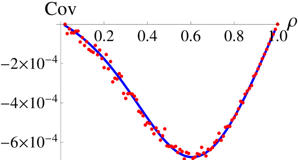
Figure 2: The exact solution of the covariance of velocities (26) is plotted versus the particle density $\rho$ for $K=100$ with $p=0.5$. Computer simulations are also performed and numerical results are dotted.

Figure 2 shows ${\rm Cov}_{L,N}[V,V^{\prime}]$ given by (26) for $K=100$ with $p=0.5$ as a function of the density of particles $\rho$. This figure shows that velocities are negatively correlated. We performed computer simulations for a variety of systems with $K=100$ and $p=0.5$ by changing the number of particles $1\leq L\leq K$. For each trial, we discarded first $2\times 10^{3}$ time-step data and used $8\times 10^{3}$ time-step data for evaluating the covariance of velocities. In Fig.2, each dot indicates the averaged value of $10^{4}$ trials. We can find that the simulation data coincide very well with the exact solution (26).

III Asymptotic Independence of Velocities

III.1 Riccati Equations

Here we consider the average velocity (10) as a function of the hopping probability $p$ and express it by

$$v_{L,N}(p)={\bf E}_{L,N}[V].$$ (29)

Kanai et al. KNT06 proved that it solves a Riccati equation

$$\frac{dv_{L,N}(p)}{dp}+\frac{L}{p(1-p)}v_{L,N}(p)^{2}-\frac{L+N}{p(1-p)}v_{L,N}(p)+\frac{N}{1-p}=0.$$ (30)

From this equation, the thermodynamic limit (13) was concluded. (See also (36) below.)

We have found that $Y_{L,N}(p)$ defined by (28) also solves a Riccati equation in the form

$$\frac{dY_{L,N}(p)}{dp}+\frac{L-1}{p}\frac{v_{L-1,N}(p)}{v_{L,N}(p)}Y_{L,N}(p)^{2}$$

$$\qquad+\left[\frac{d}{dp}\log\frac{v_{L-1,N}(p)}{v_{L,N}(p)}+\frac{2(L-1)p-(L+N-1)}{p(1-p)}\right]Y_{L,N}(p)$$

$$\qquad\qquad\qquad-\frac{L-1}{1-p}\frac{v_{L,N}(p)}{v_{L-1,N}(p)}=0.$$ (31)

The derivation is given in Appendix A. Note that by (30) we obtain the equation

$$\frac{d}{dp}\log\frac{v_{L-1,N}(p)}{v_{L,N}(p)}=\frac{dv_{L-1,N}(p)/dp}{v_{L-1,N}(p)}-\frac{dv_{L,N}(p)/dp}{v_{L,N}(p)}$$

$$=-\frac{1}{p(1-p)}\left[(L-1)v_{L-1,N}(p)-Lv_{L,N}(p)+1+Np\left(\frac{1}{v_{L-1,N}(p)}-\frac{1}{v_{L,N}(p)}\right)\right].$$ (32)

That is, the Riccati equation (31) for $Y_{L,N}(p)$, which governs ${\rm Cov}_{L,N}[V,V^{\prime}]$ through (27), is coupled with the Riccati equations (30) for $v_{L,N}(p)$ and $v_{L-1,N}(p)$.

III.2 Large-size expansion and thermodynamic limit

Following the procedure given by KNT06 , we consider the power expansion of the quantities with respect to the inverse of system size, $1/K$ with $K=L+N$,

$$v_{L,N}(p)=v_{0}+v_{1}\frac{1}{K}+v_{2}\frac{1}{K^{2}}+\cdots,$$ (33)

$$v_{L-1,N}(p)=v_{0}^{\prime}+v_{1}^{\prime}\frac{1}{K}+v_{2}^{\prime}\frac{1}{K^{2}}+\cdots,$$ (34)

$$Y_{L,N}(p)=Y_{0}+Y_{1}\frac{1}{K}+Y_{2}\frac{1}{K^{2}}+\cdots,$$ (35)

where the coefficients $v_{i},v_{i}^{\prime},Y_{i},i=0,1,2,\dots$ are assumed to be functions of $p$ and $\rho$. Putting (33) and (34) into (30) and its modification obtained by setting $L\to L-1$, and taking the thermodynamic limit $K\to\infty$ with $\rho=L/K=$ const., the first terms in (33) and (34) are determined as KNT06

$$v_{0}=v_{0}^{\prime}=\frac{1-\sqrt{1-4p\rho(1-\rho)}}{2\rho}.$$ (36)

This result implies (13).

Similarly, we put (33)-(35) into (31) with (32). In the thermodynamic limit, the differential equation is reduced to the algebraic equation

$$\rho(1-p)Y_{0}^{2}-(1-2p\rho)Y_{0}-\rho p=0$$

for $Y_{0}$, which is solved as

$$Y_{0}=\lim_{\begin{subarray}{c}K\to\infty;\\ \rho={\rm const.}\end{subarray}}Y_{L,N}(p)=\frac{(1-2\rho p)\pm\sqrt{1-4\rho p(1-\rho)}}{2\rho(1-p)}.$$ (37)

On the other hand, in the similar way, we can show that (27) gives

$$\lim_{\begin{subarray}{c}K\to\infty;\\ \rho={\rm const.}\end{subarray}}{\rm Cov}_{L,N}[V,V^{\prime}]=p(1-p)+\left[\frac{1-2\rho p}{2\rho}\right]^{2}-\left[(1-p)Y_{0}-\left(\frac{1-2\rho p}{2\rho}\right)\right]^{2}.$$ (38)

If we apply the result (37), (38) turns to be

$$\lim_{\begin{subarray}{c}K\to\infty;\\ \rho={\rm const.}\end{subarray}}{\rm Cov}_{L,N}[V,V^{\prime}] = p(1-p)+\left[\frac{1-2\rho p}{2\rho}\right]^{2}-\frac{1-4\rho p(1-\rho)}{4\rho^{2}}$$ (39)

$$= 0.$$

Vanishing of the covariance implies that velocities of particles of the discrete-time TASEP become independent asymptotically in the thermodynamic limit in the stationary state on a circle.

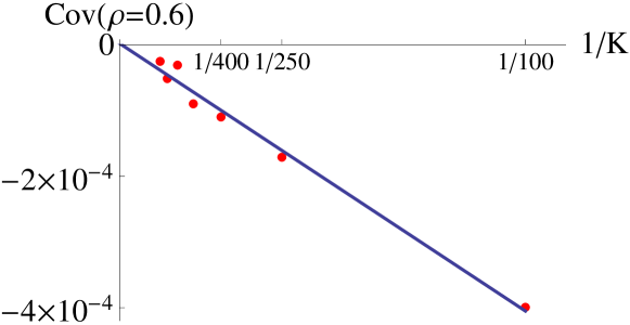
Figure 3: Numerical fitting of ${\rm Cov}_{L,N}[V,V^{\prime}]$ evaluated by computer simulations versus $1/K$ for $p=0.5,\rho=0.6$. The data shows that ${\rm Cov}_{L,N}[V,V^{\prime}]$ becomes zero as $K=L+N\to\infty$ in the form (40) with $c(p=0.5,\rho=0.6)\simeq-4\times 10^{-2}$. In each trial of computer simulation, we discarded first $2\times 10^{4}$ time-step data and used $10^{4}$ time-step data for evaluating the covariance of velocities and each dot in this figure indicates the averaged value over $10^{4}$ trials.

Figure 3 shows the numerical data demonstrating ${\rm Cov}_{L,N}[V,V^{\prime}]\to 0$ as $K=L+N\to\infty$. Here we set $p=0.5$ and $\rho=0.6$ and performed computer simulations by increasing $K$ from 100 to 1000 by 150, in which ${\rm Cov}_{L,N}[V,V^{\prime}]$ with $L=\rho K$ and $N=(1-\rho)K$ are evaluated. The linear fitting of ${\rm Cov}_{L,N}[V,V^{\prime}]$ versus $1/K$ gives

$${\rm Cov}_{L,N}[V,V^{\prime}]\simeq\frac{c(p,\rho)}{K}$$ (40)

with $c(p=0.5,\rho=0.6)\simeq-4\times 10^{-2}$.

IV Concluding Remarks

In the present paper, we study a discrete-time version of the TASEP on a circle developed by the parallel update rule. This version is easily simulated by a computer. As a matter of fact, we have checked the validity of our exact solutions for finite-size systems by comparing them with the numerical simulation data as shown by Fig.2.

From the viewpoint of statistical mechanics, it is important to discuss the thermodynamic limit for non-equilibrium steady states realized in the present model. It is rather difficult, however, to define parallel update dynamics for a system with an infinite number of particles, since the number of updated sites can be infinity, i.e., $|\widehat{A_{t}}|=\infty$ using the notation in Sec.I. Kanai et al.KNT06 overcame this difficulty and determined the thermodynamic limit of average velocity (13). They obtained the differential equation which governs the average velocity and took the thermodynamic limit in the equation. In the present paper, we extend their procedure for the covariance of two-particle velocities and showed that it becomes asymptotically zero in the thermodynamic limit (39).

It should be remarked that both equations which govern the average velocity and the covariance are given by the Riccati-type differential equations with respect to the hopping probability $p$. As a matter of course, the Riccati equation (31) for $Y_{L,N}(p)$, which governs ${\rm Cov}_{L,N}[V,V^{\prime}]$ through (27), is coupled with the equations (30) for the average velocities (see (32)), and thus it becomes much complicated. Further study of hierarchy in the coupled system of differential equations which determine the third and higher-order moments of velocities will be an interesting future problem.

Appendix A Derivation of Riccati equation (31)

By definitions (28) and (29) with (10),

$$\frac{v_{L-1,N}(p)}{v_{L,N}(p)}Y_{L,N}(p)=\frac{F(L-1,N;1,z)}{F(L,N;1,z)},$$ (41)

where we put

$$z=\frac{1}{1-p}.$$ (42)

By the following formula of the Gauss hypergeometric function AS72

$$\frac{d}{dz}\left[\frac{(1-z)^{L+N-1}}{z^{L-1}}F(L,N;1;z)\right]=(1-L)\frac{(1-z)^{L+N-2}}{z^{L}}F(L-1,N;1;z),$$

(41) is written as

$$\frac{v_{L-1,N}(p)}{v_{L,N}(p)}Y_{L,N}(p)=\frac{z(1-z)}{1-L}\frac{1}{w(z)}\frac{dw(z)}{dz}$$ (43)

with

$$w(z)=\frac{(1-z)^{L+N-1}}{z^{L-1}}F(L,N;1;z).$$ (44)

Here we consider the generalized hypergeometric differential equation

$$\frac{du(z)}{dz^{2}}+\sum_{i=1}^{3}\frac{1-\lambda_{i}-\lambda_{i}^{\prime}}{z-a_{i}}\frac{du(z)}{dz}$$

$$\qquad+\sum_{i=1}^{3}\frac{\lambda_{i}\lambda_{i}^{\prime}}{z-a_{i}}\prod_{1\leq j\leq 3;j\not=i}(a_{i}-a_{j})\frac{u(z)}{(z-a_{1})(z-a_{2})(z-a_{3})}=0,$$ (45)

where Fuchs’ relation $\sum_{i=1}^{3}(\lambda_{i}+\lambda_{i}^{\prime})=1$ is assumed to be satisfied. The solution of (45) is expressed by

$$u(z)=P\left\{\begin{array}[]{cccc}a_{1}&a_{2}&a_{3}&\cr\lambda_{1}&\lambda_{2}&\lambda_{3}&z\cr\lambda_{1}^{\prime}&\lambda_{2}^{\prime}&\lambda_{3}^{\prime}&\end{array}\right\},$$ (46)

which is called Riemann’s $P$ function AS72 . As a special case, the Gauss hypergeometric function (8) is given by

$$F(\alpha,\beta;\gamma;z)=P\left\{\begin{array}[]{cccc}0&1&\infty&\cr 0&0&\alpha&z\cr 1-\gamma&\gamma-\alpha-\beta&\beta&\end{array}\right\}.$$ (47)

In general, the following relations holds,

$$P\left\{\begin{array}[]{cccc}a_{1}&a_{2}&a_{3}&\cr\lambda_{1}&\lambda_{2}&\lambda_{3}&z\cr\lambda_{1}^{\prime}&\lambda_{2}^{\prime}&\lambda_{3}^{\prime}&\end{array}\right\} = P\left\{\begin{array}[]{cccc}a_{2}&a_{1}&a_{3}&\cr\lambda_{2}&\lambda_{1}&\lambda_{3}&z\cr\lambda_{2}^{\prime}&\lambda_{1}^{\prime}&\lambda_{3}^{\prime}&\end{array}\right\},$$ (54)

$$(z-a_{1})^{k}P\left\{\begin{array}[]{cccc}a_{1}&a_{2}&\infty&\cr\lambda_{1}&\lambda_{2}&\lambda_{3}&z\cr\lambda_{1}^{\prime}&\lambda_{2}^{\prime}&\lambda_{3}^{\prime}&\end{array}\right\} = P\left\{\begin{array}[]{cccc}a_{1}&a_{2}&\infty&\cr\lambda_{1}+k&\lambda_{2}&\lambda_{3}-k&z\cr\lambda_{1}^{\prime}+k&\lambda_{2}^{\prime}&\lambda_{3}^{\prime}-k&\end{array}\right\}.$$ (61)

By (47), (44) is written as

$$w(z)=(-1)^{L+N-1}(z-1)^{L+N-1}z^{1-L}P\left\{\begin{array}[]{cccc}0&1&\infty&\cr 0&0&L&z\cr 0&1-L-N&N&\end{array}\right\}.$$

Using the relations (54) and (61), we can show that

$$w(z)=P\left\{\begin{array}[]{cccc}0&1&\infty&\cr 1-L&L+N-1&L-N&z\cr 1-L&0&0&\end{array}\right\}.$$ (62)

It implies that $w(z)$ solves the differential equation

$$\frac{d^{2}w(z)}{dz^{2}}-\frac{(L-N+1)z-2L+1}{(1-z)z}\frac{dw(z)}{dz}+\frac{(L-1)^{2}}{(1-z)z^{2}}w(z)=0.$$ (63)

Since $dw(z)/dz$ is related with $Y_{L,N}(p)$ by (43), (63) gives the first-order differential equation for $Y_{L,N}(p)$. By straightforward calculation, (31) is derived.

References

- (1) T. M. Liggett, Interacting Particle Systems, (Springer, New York, 1985).
- (2) H. Spohn, Large Scale Dynamics of Interacting Particles, (Springer, Berlin, 1991).
- (3) B. Schmittmann, R. K. P. Zia, Statistical Mechanics of Driven Diffusive Systems, in: ed. C. Domb and J. L. Lebowitz, Phase Transitions and Critical Phenomena, vol.17, (Academic Press, New York, 1995).
- (4) T. M. Liggett, Stochastic Interacting Systems: Contact, Voter, and Exclusion Processes, (Springer, Berlin, 1999).
- (5) G. M. Schütz, Exactly Solvable Models for Many-Body Systems Far From Equilibrium, in: ed. C. Domb and J. L. Lebowitz, Phase Transitions and Critical Phenomena, vol.19, (Academic Press, New York, 2000).
- (6) R. Mahnke, J. Kaupužs, I. Lubashevsky, Physics of Stochastic Processes: How Randomness Acts in Time, (Wiley-VCH, Germany, 2009).
- (7) N. Rajewsky, L. Santen, A. Schadschneider, M. Schreckenberg, J. Stat. Phys. 92, 151 (1998).
- (8) M. R. Evans, Braz. J. Phys. 30, 42 (2000).
- (9) M. R. Evans, T. Hanney, J. Phys. A: Math. Gen. 38, R195 (2005).
- (10) M. Kanai, K. Nishinari, T. Tokihiro, J. Phys. A: Math. Gen. 39, 9071 (2006).
- (11) M. Kanai, J. Phys. A: Math. Gen. 40, 7127 (2007).
- (12) M. R. Evans, J. Phys. A: Math. Gen. 30, 5669 (1997).
- (13) If we set for and , the values of and can be arbitrarily chosen without changing given by (5). In KNT06 , they are chosen as . Here we simply set .
- (14) M. Abramowitz, I. A. Stegun, Handbook of Mathematical Functions with Formulas, Graphs, and Mathematical Tables, (Dover, New York, 1972).
- (15) A. Schadschneider, M. Schreckenberg, J. Phys. A: Math. Gen. 26, L679 (1993).