Neutrino energy loss rates and positron capture rates on ⁵⁵Co for presupernova and supernova physics

Abstract

Proton-neutron quasi-particle random phase approximation (pn-QRPA) theory has recently being used for calculation of stellar weak interaction rates of $fp$-shell nuclide with success. Neutrino losses from proto-neutron stars play a pivotal role to decide if these stars would be crushed into black holes or explode as supernovae. The product of abundance and positron capture rates on ⁵⁵Co is substantial and as such can play a role in fine tuning of input parameters of simulation codes specially in the presupernova evolution. Recently we introduced our calculation of capture rates on ⁵⁵Co, in a luxurious model space of $7\hbar\omega$, employing the pn-QRPA theory with a separable interaction. Simulators, however, may require these rates on a fine scale. Here we present for the first time an expanded calculation of the neutrino energy loss rates and positron capture rates on ⁵⁵Co on an extensive temperature-density scale. These type of scale is appropriate for interpolation purposes and of greater utility for simulation codes. The pn-QRPA calculated neutrino energy loss rates are enhanced roughly up to two orders of magnitude compared with the large-scale shell model calculations and favor a lower entropy for the core of massive stars. PACS numbers: 21.60.Jz, 23.40.Bw, 26.30.Jk, 26.50.+x

I Introduction

Supernovae are nature’s grandest explosions. They are also responsible for synthesizing most of the elements of nature, including those that form our own planet, Earth. Many exotic states of matter, including black holes and neutron stars, also owe their existence to supernovae. Since 1934, when Baade and Zwicky [1] suggested that supernovae are energized by the collapse of an ordinary star to a neutron star, scientists started debating about the physical mechanism responsible for these spectacular explosions (where the luminosity of the star becomes comparable to that of an entire galaxy containing around $10^{11}$ stars$!$). Whereas gravity remains the undisputed source of energy, the relative roles of other physical phenomena including, but not limited to, roles of neutrino, continue to be argued.

The evolution of a massive star (of masses above $10M_{\odot}$) comprises of several stages including hydrogen, helium, carbon, neon, oxygen and silicon burning. The time scales, temperatures, densities, fuels, luminosities and neutrino losses for these stages can be found in Ref. [2]. During the late phases of evolution of these massive stars an iron core develops (of mass around $1.5M_{\odot}$). The binding energy per nucleon curve prohibits any further production of energy by nuclear fusion, yet the neutrino losses continue unabated, exceeding the Sun’s luminosity by a factor of about $10^{15}$. Capture rates and photodisintegration processes contribute in the lowering of the degeneracy pressure required to counter the enormous self-gravity force of the star. Under such extreme thermodynamic conditions, neutrinos are produced in abundance. Eventually the collapse of the iron core begins. The mechanism of core-collapse supernovae is strongly believed to depend upon the transfer of energy from the inner core to the outer mantle of the iron core. Neutrinos seem to be the mediators of this energy transfer. The shock wave, produced as a result, stalls due to photodisintegration and neutrino energy losses. Once again the part played by neutrinos in this scenario is far from being completely understood. Whereas Haxton [3] proposed the mechanism of ”preheating” by neutrinos as a means of assistance for shock revival, Bruenn and Haxton [4] later discouraged the preheating mechanism. They worked on two different models, simulating weak and strong shock cases, and found out that in neither case is the energy transferred to the matter by neutrino-nucleus absorption significant in terms of preheating the infalling iron-like material. More recently, Langanke and collaborators [5] had some observations on the models of Bruenn and Haxton [4] and reported much larger preshock heating rates, albeit acting for too short a time to lead to consequences for shock propagation. According to authors in Ref. [5] the inelastic neutrino-nucleus scattering modifies the radiated neutrino spectra and strongly reduces the high-energy spectral tail of the electron neutrino burst at shock breakout.

A few milliseconds after the bounce, the proto-neutron star accretes mass at a few tenths of solar mass per second. This accretion, if continued even for one second, can change the ultimate fate of the collapsing core resulting into a black hole. Neutrinos are the main characters in this play and radiate around 10$\%$ of the rest mass converting the star to a neutron star (e.g. [2]). Despite the small neutrino-nucleus cross sections, the neutrinos flux generated by the cooling of a neutron star can produce a number of nuclear transmutations as it passes the onion-like structured envelope surrounding the neutron star. Within $\sim$ 0.1 s of the beginning of the collapse the nonthermal neutrino emission is dominated by electron neutrinos owing to the decay and capture of leptons by nuclei and free protons. The mean individual neutrino energies are some $\sim$ 10 MeV and constitute roughly 10$\%$ of the total available energy of around $(3-5)$x $10^{53}$ erg [6].

The neutrino energy loss rates are important input parameters in multi-dimensional simulations of the contracting proto-neutron star. The reenergizing by charged-current electron neutrino and antineutrino absorption on the dissociation-liberated protons and neutrons in the postshock flow remains integral to the supernova paradigm and neutrino transport is arguably the single most important component of any supernova model [7]. (For a review of supernova neutrino microphysics see also Ref. [8].) Parameter-free multi-dimensional models, with neutrino transport included consistently throughout the entire mass, yield conflicting results on the key issue of whether the star actually explodes. Reliable and microscopic calculations of neutrino loss rates and capture rates can contribute effectively in the final outcome of these simulations on world’s fastest supercomputers.

During core infall electron neutrinos are produced almost entirely by electron captures on free protons and nuclei and at sufficiently high temperatures antineutrinos are also produced as a result of positron captures on neutrons. Electron capture on protons and positron capture on neutrons also play a crucial role in the evolution of star and supernova explosion. During the collapse and accretion phases, they decrease the degenerate pressure in the stellar core. The neutrinos produced in these capture processes carry the energy away and result in the lowering of the entropy of the core. Positron captures are of great importance in high temperature and low density locations. In such conditions, a rather high concentration of positrons can be reached from $e^{-}+e^{+}\leftrightarrow\gamma+\gamma$ equilibrium favoring the $e^{-}e^{+}$ pairs. Positron capture on elements lying at the bottom of the valley of nuclear beta-stability (so-called s elements) may capture positrons and be transformed into a proton-rich isobars (so-called p elements). The electron capture on proton and the positron capture on neutron are considered important ingredients in the modelling of Type-II supernovae [9].

Fuller, Fowler, and Newman (FFN) [10] performed the first-ever extensive calculation of stellar weak rates including the capture rates, neutrino energy loss rates and decay rates for a wide density and temperature domain. They made this detailed calculations for 226 nuclei in the mass range $21\leq A\leq 60$. They also stressed the importance of the Gamow-Teller (GT) giant resonance strength in the capture of the electron and estimated the GT centroids using zeroth-order ($0\hbar\omega$ ) shell model. Later, Aufderheide et al. [11] extended the FFN work for heavier nuclei with A $>$ 60. They tabulated the 90 top electron capture nuclei averaged throughout the stellar trajectory for $0.40\leq Ye\leq 0.5$ (see Table. 25 therein). Since then theoretical efforts were concentrated on the microscopic calculations of capture rates of iron-regime nuclide. Large-scale shell model (e.g. [12]) and the proton-neutron quasiparticle random phase approximation theory (pn-QRPA) (e.g. [13]) were used extensively and with relative success for the microscopic calculation of stellar capture rates and neutrino energy losses. Monte Carlo shell-model is an alternative to the diagonalization method and allows calculation of nuclear properties as thermal averages (e.g. [14]). However it does not allow for detailed nuclear spectroscopy.

Nabi and Klapdor [15] calculated weak interaction rates for 709 nuclei with A = 18 to 100 in stellar matter using the pn-QRPA theory. These included capture rates, decay rates, neutrino energy loss rates, probabilities of beta-delayed particle emissions and energy rate of these particle emissions. Since then these calculations were further refined with use of more efficient algorithms, incorporation of latest data from mass compilations and experimental values, and fine-tuning of model parameters [16, 17, 18, 19].

⁵⁵Co is abundant in the presupernova conditions and is thought to contribute effectively in the dynamics of presupernova evolution. Aufderheide and collaborators [11] placed ⁵⁵Co among the list of top ten most important capture nuclei during the presupernova evolution. Later Heger et al. [20] also identified ⁵⁵Co as the most important nuclide for capture purposes for massive stars ($25M_{\odot}$). Realizing the importance of ⁵⁵Co in astrophysical environments, Nabi, Rahman and Sajjad [21] reported the calculation of electron and positron capture rates on ⁵⁵Co using the pn-QRPA theory (see also Ref. [22]). However there was a need to perform a fine calculation of these important capture rates on a detailed temperature-density grid suitable for collapse simulation codes (see, for example, Ref. [18, 23]). Due to the extreme conditions prevailing in these scenarios, interpolation of calculated rates within large intervals of temperature-density points posed some uncertainty in the values of capture rates for collapse simulators. Further, as mentioned above, the neutrino energy loss rates needed to be included in these expanded calculations on a detailed stellar temperature-density grid to make them more useful in simulation codes.

In this paper we present for the first time an expanded calculation of (anti)neutrino energy loss rates and positron capture rates on ⁵⁵Co at fine intervals of temperature-density intervals. Section II deals with the formalism of our calculation. Due to existing physical situation and lack of experimental data the uncertainties present in stellar rate calculations are considerable. We discuss the uncertainties of the pn-QRPA model in Section III. In Section IV we will be presenting some of our results. Comparisons with earlier calculations are also included in this section. We finally will be concluding in Section V and at the end Table V presents our expanded calculation of (anti)neutrino energy loss rates and positron capture rates on ⁵⁵Co.

II The quasi-particle random phase approximation with a separable interaction

The QRPA theory is an efficient way to generate GT strength distributions. These strength distributions constitute a primary and non-trivial contribution to the calculation of positron capture and neutrino energy loss rates. Kar et al. [24] pointed out that the quasiparticle random phase approximation (QRPA) method is quite successful in predicting the weak interaction rates of ground states all over the periodic table and also stressed the need to extend these methods to non-zero temperature domains relevant to presupernova and supernova conditions. QRPA is also the method of choice in dealing heavy nuclei [25]. The QRPA theory considers the residual correlations among the nucleons via one particle one hole (1p-1h) excitations in a large model space. Nabi and Klapdor [15] extended the QRPA model to configurations more complex than 1p-1h.

We used the pn-QRPA theory to calculate the GT strength functions and the associated capture and neutrino energy loss rates for ⁵⁵Co. The reliability of the pn-QRPA calculations was discussed in detail by Nabi and Klapdor [13]. There the authors compared the measured data (half lives and B(GT) strength) of thousands of nuclide with the pn-QRPA calculations and got fairly good comparison. We incorporated experimental data wherever available to further strengthen the reliability of our calculated rates. The calculated excitation energies (along with their log ft values) were replaced with the experimental ones when they were within 0.5 MeV of each other. Missing measured states were inserted and inverse and mirror transitions were also taken into account. We did not replace the theoretical levels with the experimental ones beyond the excitation energy for which experimental compilations had no definite spin and/or parity assignment (2.98 MeV in case of ⁵⁵Co). The pn-QRPA theory was used with a separable interaction which granted us the liberty of performing the calculations in a much larger single-particle basis than a general interaction. We performed the pn-QRPA calculations using a model space of seven major harmonic oscillator shells ($7\hbar\omega$). The Hamiltonian for our calculations was of the form

$$H^{QRPA}=H^{sp}+V^{pair}+V_{GT}^{ph}+V_{GT}^{pp},$$ (1)

here $H^{sp}$ is the single-particle Hamiltonian, $V^{pair}$ is the pairing force, $V_{GT}^{ph}$ is the particle-hole (ph) Gamow-Teller force, and $V_{GT}^{pp}$ is the particle-particle (pp) Gamow-Teller force. Single particle energies and wave functions were calculated in the Nilsson model, which takes into account nuclear deformations. Pairing was treated in the BCS approximation. The proton-neutron residual interactions occurred as particle-hole and particle-particle interaction. The interactions were given separable form and were characterized by two interaction constants $\chi$ and $\kappa$, respectively. The selections of these two constants were done in an optimal fashion. For details of the fine tuning of the Gamow-Teller strength parameters, we refer to Ref. [26, 27]. In this work, we took the values of $\chi=0.2MeV$ and $\kappa=0.07MeV$. Other parameters required for the calculation of weak rates are the Nilsson potential parameters, the deformation, the pairing gaps, and the Q-value of the reaction. Nilsson-potential parameters were taken from Ref. [28] and the Nilsson oscillator constant was chosen as $\hbar\omega=41A^{-1/3}(MeV)$ (the same for protons and neutrons). The calculated half-lives depend only weakly on the values of the pairing gaps [29]. Thus, the traditional choice of $\Delta_{p}=\Delta_{n}=12/\sqrt{A}(MeV)$ was applied in the present work. The deformation parameter for ⁵⁵Co, $\delta$, was taken to be 0.06, according to Möller and Nix [30]. (See also the discussion on choice of deformation parameter in Ref. [19].) Q-values were taken from the recent mass compilation of Audi et al. [31].

The positron capture rates of a transition from the $ith$ state of the parent to the $jth$ state of the daughter nucleus is given by

$$\lambda^{{}^{pc}}_{ij}=\left[\frac{\ln 2}{D}\right]\left[f_{ij}^{pc}(T,\rho,E_{f})\right]\left[B(F)_{ij}+\left({\raise 3.01385pt\hbox{$g_{A}$}\!\mathord{\left/{\vphantom{g_{A}g_{V}}}\right.\kern-1.2pt}\!\lower 3.01385pt\hbox{$g_{V}$}}\right)^{2}B(GT)_{ij}\right].$$ (2)

We took the value of D=6295s [32] and the ratio of the axial vector to the vector coupling constant as -1.254 [33]. $B_{ij}^{\prime}$s are the sum of reduced transition probabilities of the Fermi B(F) and GT transitions B(GT). Details of these reduced transition probabilities can be found in Ref. [13, 17]. The phase space integral $f_{ij}$ is an integral over total energy and for positron capture it is given by

$$f_{ij}^{pc}\,=\,\int_{w_{l}}^{\infty}w\sqrt{w^{2}-1}(w_{m}\,+\,w)^{2}F(-Z,w)G_{+}dw.$$ (3)

In above equation $w$ is the total energy of the electron including its rest mass, $w_{l}$ is the total capture threshold energy (rest+kinetic) for positron capture. F(-Z,w) are the Fermi functions and were calculated according to the procedure adopted by Gove and Martin [34]. G₊ is the Fermi-Dirac distribution function for positrons.

$$G_{+}=\left[\exp\left(\frac{E+2+E_{f}}{kT}\right)+1\right]^{-1},$$ (4)

here $E=(w-1)$ is the kinetic energy of the positrons, $E_{f}$ is the Fermi energy of the positrons, $T$ is the temperature, and $k$ is the Boltzmann constant.

The number density of electrons associated with protons and nuclei is $\rho Y_{e}N_{A}$ ($\rho$ is the baryon density, $Y_{e}$ is lepton to baryon ratio, and $N_{A}$ is Avogadro’s number)

$$\rho Y_{e}=\frac{1}{\pi^{2}N_{A}}(\frac{m_{e}c}{\hbar})^{3}\int_{0}^{\infty}(G_{-}-G_{+})p^{2}dp,$$ (5)

here $p=(w^{2}-1)^{1/2}$ is the positron momentum and Eqt. (5) has the units of $mol\hskip 7.22743ptcm^{-3}$. G_- is the Fermi-Dirac distribution function for electrons.

$$G_{-}=\left[\exp\left(\frac{E-E_{f}}{kT}\right)+1\right]^{-1}.$$ (6)

Eqt.5 was used for an iterative calculation of Fermi energies for selected values of $Y_{e}$ and T. There is a finite probability of occupation of parent excited states in the stellar environment as result of the high temperature prevailing in the interior of massive stars. Weak interactions then also have a finite contribution from these excited states. The total positron capture rate per unit time per nucleus is given by

$$\lambda_{pc}=\sum_{ij}P_{i}\lambda_{ij}^{pc}.$$ (7)

The summation over all initial and final states was carried out until satisfactory convergence in the rate calculations was achieved. Here $P_{i}$ is the probability of occupation of parent excited states and follows the normal Boltzmann distribution.

The neutrino energy loss rates can occur through four different weak-interaction mediated channels: electron and positron emissions, and, continuum electron and positron captures. The neutrino energy loss rates were calculated using the same formalism described above except that the phase space integral was replaced by

$$f_{ij}^{\nu}\,=\,\int_{l}^{w_{m}}w\sqrt{w^{2}-1}(w_{m}\,-\,w)^{3}F(\pm Z,w)(1-G_{\mp})dw,$$ (8)

and by

$$f_{ij}^{\nu}\,=\,\int_{w_{l}}^{\infty}w\sqrt{w^{2}-1}(w_{m}\,+\,w)^{3}F(-Z,w)G_{+}dw.$$ (9)

For the decay channel Eqt. 8 was used for the calculation of phase space integrals. Upper signs were used for the case of electron emissions and lower signs for the case of positron emissions. Regarding the capture channels, Eqt. 9 was used for the calculation of phase space integrals keeping upper signs for continuum electron captures and lower signs for continuum positron captures.

The total neutrino energy loss rate per unit time per nucleus is given by

$$\lambda_{\nu}=\sum_{ij}P_{i}\lambda_{ij}^{\nu},$$ (10)

where $\lambda_{ij}^{\nu}$ is the sum of the electron capture and positron decay rates for the transition $i\rightarrow j$.

On the other hand the total antineutrino energy loss rate per unit time per nucleus is given by

$$\lambda_{\bar{\nu}}=\sum_{ij}P_{i}\lambda_{ij}^{\bar{\nu}},$$ (11)

where $\lambda_{ij}^{\bar{\nu}}$ is the sum of the positron capture and electron decay rates for the transition $i\rightarrow j$.

III Uncertainties of the pn-QRPA model

The uncertainties involved in stellar rate calculations are considerable. The prevailing extreme physical conditions and model parameters invoke uncertainties in the calculation. Lack of experimental data in this scenario deteriorates the situation. The “electron capture direction” can be explored experimentally by (n,p) experiments whereas the “beta minus decay direction” can be explored by the (p,n) reactions. There are a handful of other experiments which have been used by many theorists to shape the centroid and width of the GT strength. However these experimental data are not enough to completely explore the domain of nuclei which are interesting from astrophysical viewpoint. There is no experimental data concerning GT strength distribution from parent excited states. In the stellar environment, at high temperatures and densities, there is a finite probability of occupation of parent excited states and transitions from these excited states are sometimes many orders of magnitude higher than transitions from ground states [19]. The weak interaction rates are calculated using

$$\lambda_{ij}=\frac{ln2}{D}f_{ij}B_{ij}.$$ (12)

Here $i$ represents the parent excited states and $j$ the daughter’s. The first factor is a constant and the second are phase space integrals which can be calculated relatively accurate. It is the third factor (the reduced transition probabilities) which contains interesting nuclear physics and incorporates uncertainties in the model. Again the reduced transition probabilities is a sum of Fermi and GT component (see Eqt. 2). Whereas the calculation of Fermi transition is rather straightforward it is precisely the calculation of the excited states and reduced transition probabilities of the GT transitions which is the main cause of uncertainty of the underlying model. The pn-QRPA model constructs parent and daughter excited states and also calculates GT strength distribution among these states in a microscopic fashion. In other words the Brink’s hypothesis is not employed in this calculation which increases the reliability of the pn-QRPA calculations (Brink’s hypothesis states that GT strength distribution on excited states is identical to that from ground state, shifted only by the excitation energy of the state). As mentioned above there are still uncertainties present due to the parameters of the model. Roughly, the parameters of the pn-QRPA model can be divided into two different groups: (i) ”internal” parameters of the model which are by some means adjustable (the pairing gaps and the GT strength parameters) and (ii) ”external” parameters for which input from other sources like mass formulae (or experimental data, if available) is necessary (these include single particle energies and wavefunctions, deformations, Q values and neutron/proton separation energies). Whereas ”internal” parameters are of minor importance the uncertainty in the ”external” parameters must be viewed as the limiting factor for the calculation of weak interaction rates of unstable nuclide. The values taken for these parameters and their optimal selection procedure were highlighted in the previous section. In order to further increase the reliability of the calculated rates experimental data were incorporated into the model as also discussed in the previous section.

We, however, do have a reasonable amount of experimental data on measured half-lives and as such the pn-QRPA theory was tested to check the accuracy of the model against the experimentally known half-lives using the same set of parameters. The check was performed in both ”beta minus decay” and ”electron capture” directions.

In Tables (I) and (II), $N$ denotes the number of experimentally known half-lives shorter than the limit in the second column, $n$ is the number (and percentage) of isotopes reproduced under the condition given in the first column, and $\bar{x}$ is the average deviation defined by

$$\bar{x}=\frac{1}{n}\sum_{i=1}^{n}x_{i},$$ (13)

where
                              $x_{i}=T^{cal}_{1/2}/T^{exp}_{1/2}$    if    $T^{cal}_{1/2}\geq T^{exp}_{1/2}$

                              $x_{i}=T^{exp}_{1/2}/T^{cal}_{1/2}$    if    $T^{cal}_{1/2}<T^{exp}_{1/2}$.

($T^{cal}_{1/2}$ is the calculated half-life using the pn-QRPA model and $T^{exp}_{1/2}$ is the corresponding measured half-life.) For example, the pn-QRPA reproduces 93$\%$ of all experimentally known half-lives shorter than 1 minute for $\beta^{+}$/EC within a factor of 10 with an average deviation of $\bar{x}$ = 1.718 and 95$\%$ of all known $\beta^{-}$-decaying nuclei with half-lives less than a minute are reproduced within a factor of 5 with an average deviation of $\bar{x}$ = 1.56. It can be seen from the tables that the model works better with increasing neutron excess (corresponding to shorter half-lives), that is, with increasing distance from stability. This is in agreement with the expectation, since forbidden transitions is neglected in the calculation. This is also a promising feature with respect to the prediction of unknown half-lives (specially for unstable isotopes), implying that the predictions are made on the basis of a realistic physical model (see also Table I and Table J of Ref. [13] for predictive power of pn-QRPA in ”electron capture” direction, and Table K of Ref. [13] for the predictive power of the model in the ”beta minus decay” direction).

IV Results and comparison

At temperatures pertinent to supernova environment we have a finite probability of occupation of excited states and a microscopic calculation of rates from these excited states is desirable. Earlier, Nabi and Sajjad [19] did point to the fact that the Brink’s hypothesis ( and back resonances for calculation of beta decay rates) is not a good approximation to use in stellar rate calculations. Brink’s hypothesis states that GT strength distribution on excited states is identical to that from ground state, shifted only by the excitation energy of the state whereas the GT back resonances are states reached by the strong GT transitions in the electron capture process built on ground and excited states. The luxury of having a huge model space at our disposal allowed us to perform the calculation of electron capture rates from 30 excited states of ⁵⁵Co. Table III shows the calculated excited states of ⁵⁵Co using the pn-QRPA theory. For each parent state we calculated the GT strength distribution in a microscopic fashion to around 200 excited states in daughter.

The GT strength distribution ($GT_{\pm}$) from ground state and first two excited states of ⁵⁵Co was presented earlier [21]. We calculated the position of our GT_- (in this direction a neutron is changed into a proton) centroid around 9.1 MeV for the ground state. For the first two excited states of ⁵⁵Co ($@$ 2.2 MeV and 2.6 MeV), the corresponding centroids were placed at 9.2 MeV and 9.6 MeV, respectively. The total GT strength for positron capture from ground state of ⁵⁵Co was calculated to be around 17.9. Table IV shows the calculated B(GT_-) strength values for the ground state of ⁵⁵Co. The strengths are given up to energy of 10 MeV in daughter nucleus, ⁵⁵Ni. Calculated B(GT_-) strength of magnitude less than $10^{-3}$ are not included in this table.

Recently, we presented the extensive calculation of electron capture rates on ⁵⁵Co on a fine temperature-density scale where we also discussed our results in detail [23]. Here we would like to present a similar calculation for the positron capture and the associated (anti)neutrino energy loss rates due to weak-interaction mediated reactions in the core of massive stars.

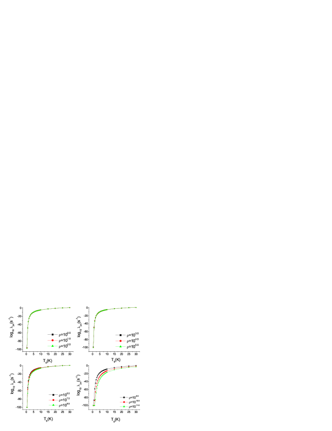
Figure 1: Positron capture rates on ⁵⁵Co, as a function of stellar temperatures, for different selected densities . Densities are in units of $gcm^{-3}$. Temperatures are measured in $10^{9}$ K and log${}_{10}\lambda_{pc}$ represents the log of positron capture rates in units of $sec^{-1}$.

Fig.1 shows four panels depicting our calculated positron capture rates at selected temperature and density domain. The upper left panel shows the positron capture rates in low-density region ($\rho[gcm^{-3}]=10^{0.5},10^{1.5}$ and $10^{2.5}$), the upper right in medium-low density region ($\rho[gcm^{-3}]=10^{3.5},10^{4.5}$ and $10^{5.5}$), the lower left in medium-high density region ($\rho[gcm^{-3}]=10^{6.5},10^{7.5}$ and $10^{8.5}$) and finally the lower right panel depicts our calculated positron capture rates in high density region ($\rho[gcm^{-3}]=10^{9.5},10^{10.5}$ and $10^{11}$). The positron capture rates are given in logarithmic scales in units of $s^{-1}$. T₉ gives the stellar temperature in units of $10^{9}$K. One should note the order of magnitude differences in positron capture rates as the stellar temperature increases. It can be seen from this figure that in the low density region the positron capture rates, as a function of stellar temperatures, are more or less superimposed on one another. This means that there is no appreciable change in the rates when increasing the density by an order of magnitude. We also observe that the positron capture rates are almost the same for the densities in the range $(10-10^{6})g/cm^{3}$. However as we go from the medium high density region to high density region these rates start to ’peel off’ from one another. Orders of magnitude difference in rates are observed (as a function of density) in high density regions. When the densities increase beyond the above stated range a decline in the positron capture rate starts. For a given density the rates increase monotonically with increasing temperatures.

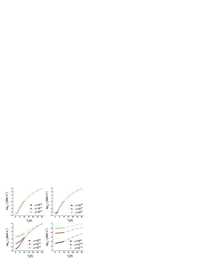
Figure 2: Neutrino energy loss rates on ⁵⁵Co, as a function of stellar temperatures, for different selected densities . Densities are in units of $gcm^{-3}$. Temperatures are measured in $10^{9}$ K and log${}_{10}\lambda_{\nu}$ represents the log of neutrino energy loss rates in units of $MeV.sec^{-1}$.

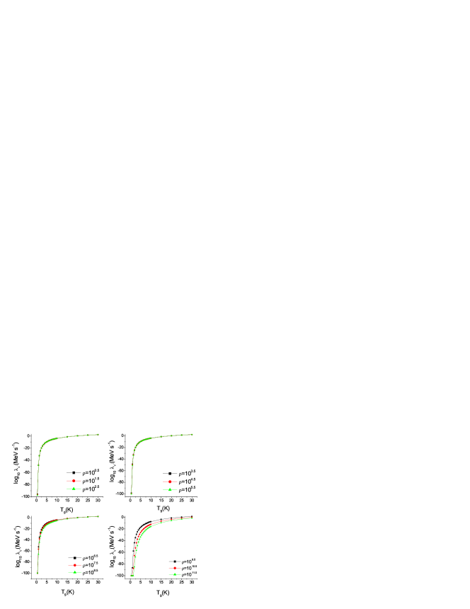
Figure 3: same as Fig.2 but for antineutrino energy loss rates.

Fig.2 and Fig.3 depict our calculated neutrino and antineutrino energy loss rates due to ⁵⁵Co. It is pertinent to mention again that the neutrino energy loss rates (depicted in Fig.2) contain contributions due to electron capture and positron decay on ⁵⁵Co whereas the antineutrino energy loss rates (Fig.3) are calculated due to contributions from positron capture and electron decay on ⁵⁵Co. The energy loss rates are given in logarithmic scales (in units of $MeV.s^{-1}$). The figures again consist of four panels depicting the low, medium-low, medium-high and high density domains for the core of a massive star. We note the similarity between the positron capture rates (Fig.1) and the antineutrino energy loss rates (Fig.3). The later are slightly enhanced at the corresponding temperature and density. On the other hand the neutrino energy loss rates exhibit an entirely different pattern. We note that the neutrino energy loss rates are orders of magnitude greater than the corresponding antineutrino energy loss rates. This is an expected result (the Q-value of ⁵⁵Co for electron capture/positron decay is 3.452 MeV whereas the Q-value of ⁵⁵Co in the other direction is -8.692 MeV [31]).

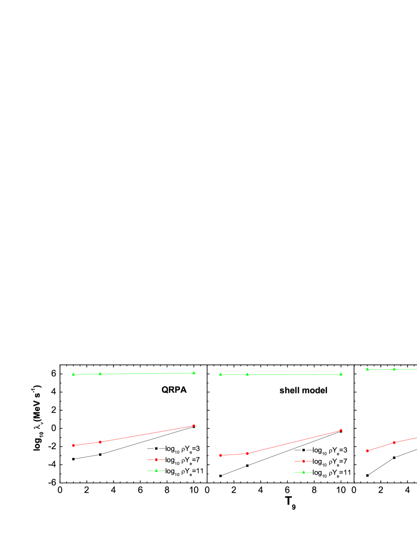
Figure 4: Comparison of neutrino energy loss rates with those of large-scale shell model [12] and FFN [10] calculations as a function of stellar temperatures and densities.

The comparison of electron and positron capture rates on ⁵⁵Co with earlier calculations were presented in Ref. [21]. Here we present a comparison of the energy loss rates with the earlier calculations. Fig.4 presents a comparison of our calculated neutrino energy loss rates compared with large-scale shell model [12] and FFN [10] calculations. The comparison is presented at densities $(10^{3},10^{7},10^{11})g.cm^{-3}$. Compared to large-scale shell model results, our calculations lead to a larger energy being carried away by the neutrinos and hence favor cooler cores. We note that our corresponding numbers are roughly as big as two orders of magnitude (at presupernova temperature and density region). In high temperature and density regions our calculated neutrino energy loss rates are in good comparison with those of large-scale shell model. As far as comparison with the pioneering work of FFN is concerned, we note that again our rates are enhanced at presupernova temperature-density domain. However at large stellar temperatures and densities, FFN neutrino energy loss rates surpass our rates. There are two main reasons for this enhancement of FFN rates. Firstly, FFN placed the centroid of the GT strength at too low excitation energies in their compilation of weak rates for odd-A and odd-odd nuclei [35]. Secondly, FFN threshold parent excitation energies were not constrained and extended well beyond the particle decay channel. At high temperatures contributions from these high excitation energies begin to show their cumulative effect. Simulators should take note of our enhanced neutrino energy loss rates at the lower temperatures and densities characteristic of the hydrostatic phases of stellar evolution which may affect the temperature and the corresponding lepton-to baryon ratio which becomes very important going into stellar collapse.

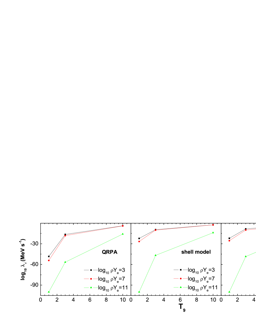
Figure 5: Same as Fig.4 but for antineutrino energy loss rates.

The story is different for the comparison of antineutrino energy loss rates (Fig.5). This time we note that the large-scale shell model rates and FFN rates are much more enhanced compared to pn-QRPA rate calculations. Nevertheless these are very small numbers and can change by orders of magnitude by a mere change of 0.5 MeV, or less, in parent or daughter excitation energies and are more indicative of the uncertainties present in the calculation of the excitation energies.

Fig.6 shows our summed GT_- strength as a function of excited states in the daughter ⁵⁵Ni. We note that almost all the strength cumulates up to an energy around 12 MeV in ⁵⁵Ni. No appreciable strength is seen in ⁵⁵Ni at higher excitation energies.

We finally present our calculated positron capture rates, neutrino and antineutrino energy loss rates on a detailed temperature-density grid in Table V. Here Column 1 shows the density in logarithmic scales (in units of $gcm^{-3}$), Column 2, the stellar temperature in units of $10^{9}K$, Column 3 gives the calculated positron capture rates in logarithmic scales (in units of $sec^{-1}$) at the corresponding temperature and density whereas Column 4 and Column 5 display the corresponding neutrino and antineutrino energy loss rates again in logarithmic scales (in units of $MeV.sec^{-1}$). All logarithms are taken to base 10. Tables of rate calculations presented in earlier compilations (e.g. Ref. [10, 12, 13, 36, 37]) were not presented on a detail temperature-density grid and at times could lead to erroneous results when interpolated. We hope that this table will prove more useful for core-collapse simulators.

V Conclusions

⁵⁵Co is advocated to play a key role amongst the iron-regime nuclide controlling the dynamics of presupernova evolution of massive stars. The capture rates and (anti)neutrino energy loss rates on ⁵⁵Co are used as nuclear physics input parameter for multi-dimensional simulations. Reliable and detailed calculations of these weak-interaction mediated rates are desirable for these codes. These parameters may fine tune the final outcome of the neutrino transport included multi-dimensional models.

Here we present, for the first time, an extensive calculation of stellar positron capture rates and the (anti)neutrino loss rates for ⁵⁵Co on a fine temperature-density scale suitable for simulation codes. According to authors in Ref. [11] and Ref. [20], ⁵⁵Co is a very important nucleus controlling the events during the pre-collapse phase of iron cores of massive stars. The calculated neutrino energy loss rates are around two orders of magnitude enhanced as compared to large-scale shell model calculations during the hydrostatic phases of stellar evolution. This may affect the temperature, entropy and the lepton-to-baryon ratio which becomes very important going into stellar collapse. We will urge simulators to test run our reported weak interaction rates presented here to check for some interesting outcome. We are currently in a phase of extending the present work for other nuclide of astrophysical importance and hope to report on the outcome of these calculations in near future.

ACKNOWLEDGMENTS

This work is partially supported by the ICTP (Italy) through the OEA-project-Prj-16.

Table (I): The accuracy of the pn-QRPA model compared to experimental data ($\beta^{+}$/EC, taken from Ref. [27]). $N$ denotes the number of experimentally known half-lives shorter than the limit in the second column, $n$ is the number (and percentage) of isotopes reproduced under the condition given in the first column, and $\bar{x}$ is the average deviation defined in the text.

Conditions	$T_{1/2}^{exp}(s)\leq$	$N$	$n$	$n(\%)$	$\bar{x}$
$\forall x_{i}\leq$ 10	106	894	706	79.0	2.057
	60	327	304	93.0	1.718
	1	81	78	96.3	1.848
$\forall x_{i}\leq$ 2	106	894	489	54.7	1.363
	60	327	245	74.9	1.308
	1	81	59	72.8	1.230

Table (II): The accuracy of the pn-QRPA model compared to experimental data ($\beta^{-}$, taken from Ref. [26]). $N$ denotes the number of experimentally known half-lives shorter than the limit in the second column, $n$ is the number (and percentage) of isotopes reproduced under the condition given in the first column, and $\bar{x}$ is the average deviation defined in the text.

Conditions	$T_{1/2}^{exp}(s)\leq$	$N$	$n$	$n(\%)$	$\bar{x}$
$\forall x_{i}\leq$ 10	106	654	472	72.2	1.85 $\pm$ 1.21
	60	325	313	96.3	1.67 $\pm$ 1.02
	1	106	105	99.1	1.44 $\pm$ 0.40
$\forall x_{i}\leq$ 5	106	654	456	69.7	1.68 $\pm$ 0.76
	60	325	307	94.5	1.56 $\pm$ 0.66
	1	106	105	99.1	1.44 $\pm$ 0.40
$\forall x_{i}\leq$ 3	106	654	420	64.2	1.50 $\pm$ 0.46
	60	325	295	90.8	1.46 $\pm$ 0.43
	1	106	105	99.1	1.44 $\pm$ 0.40
$\forall x_{i}\leq$ 2	106	654	369	56.4	1.37 $\pm$ 0.29
	60	325	267	82.2	1.36 $\pm$ 0.29
	1	106	96	90.6	1.35 $\pm$ 0.27

Table III: Calculated excited states in parent ${}^{55}Co$ using the pn-QRPA theory in units of MeV.

0.0		2.17		2.57		2.92		3.08		3.30		3.87		4.10		4.48		4.89
5.20		5.47		5.68		5.99		6.20		6.50		6.79		7.08		7.33		7.65
7.88		8.16		8.42		8.67		8.96		9.21		9.48		9.74		9.89		10.00

Table IV: Calculated B(GT_-) values from ground state in ${}^{55}Co$. The energy scale refers to excitation energies in daughter, ⁵⁵Ni.

Energy(MeV)	B(GT-)	Energy(MeV)	B(GT-)	Energy(MeV)	B(GT-)
0.00	3.06E-01	6.36	1.80E-02	8.36	5.37E-02
2.46	1.40E+00	6.66	2.91E-02	8.62	2.45E-02
3.01	4.48E-01	6.85	4.47E-02	8.73	3.78E-01
3.45	1.04E-01	7.00	1.12E-02	8.90	3.26E-01
3.57	1.80E-03	7.14	1.06E-02	9.11	2.94E+00
3.68	1.79E-01	7.43	1.19E-01	9.26	1.59E+00
3.90	1.99E-01	7.59	6.53E-03	9.42	1.00E+00
4.11	2.25E-02	7.76	8.77E-02	9.60	2.11E+00
5.82	1.93E-02	7.92	1.62E-02	9.87	4.84E-02
5.93	3.89E-03	8.04	1.92E-01	10.03	7.67E-02
6.13	1.58E-02	8.25	7.51E-02

Table V: Calculated positron capture, neutrino and antineutrino energy loss rates on ${}^{55}Co$ for different selected densities and temperatures in stellar matter. log($\rho Y_{e}$) has units of $g/cm^{3}$, where $\rho$ is the baryon density and $Y_{e}$ is the ratio of the lepton number to the baryon number. Temperatures ($T_{9}$) are measured in $10^{9}$ K. $\lambda_{pc}$ are the positron capture rates $(sec^{-1})$. $\lambda_{\nu}$ are the total neutrino energy loss rates $(MeV.s^{-1})$ due to $\beta^{+}$ decay and electron capture. $\lambda_{\bar{\nu}}$ are the total antineutrino energy loss rates $(MeV.s^{-1})$ due to $\beta^{-}$ decay and positron capture. All calculated rates are tabulated in logarithmic (to base 10) scale. In the table, -100 means that the rate is smaller than 10^-100.

$log\rho Y_{e}$	$T_{9}$	$\lambda_{pc}$	$\lambda_{\nu}$	$\lambda_{\bar{\nu}}$	$log\rho Y_{e}$	$T_{9}$	$\lambda_{pc}$	$\lambda_{\nu}$	$\lambda_{\bar{\nu}}$	$log\rho Y_{e}$	$T_{9}$	$\lambda_{pc}$	$\lambda_{\nu}$	$\lambda_{\bar{\nu}}$
0.5	0.5	-95.544	-3.375	-95.515	1	8.5	-5.531	-0.308	-5.082	2	4.5	-11.138	-2.004	-10.894
0.5	1	-48.153	-3.376	-48.102	1	9	-5.137	-0.136	-4.666	2	5	-10.008	-1.743	-9.736
0.5	1.5	-32.485	-3.366	-32.41	1	9.5	-4.776	0.03	-4.284	2	5.5	-9.067	-1.501	-8.768
0.5	2	-24.599	-3.305	-24.498	1	10	-4.442	0.191	-3.93	2	6	-8.269	-1.274	-7.942
0.5	2.5	-19.828	-3.143	-19.699	1	15	-2.053	1.571	-1.365	2	6.5	-7.579	-1.062	-7.227
0.5	3	-16.614	-2.884	-16.457	1	20	-0.553	2.584	0.264	2	7	-6.976	-0.86	-6.598
0.5	3.5	-14.292	-2.585	-14.107	1	25	0.506	3.342	1.425	2	7.5	-6.441	-0.668	-6.039
0.5	4	-12.529	-2.287	-12.315	1	30	1.301	3.933	2.304	2	8	-5.963	-0.484	-5.537
0.5	4.5	-11.138	-2.006	-10.896	1.5	0.5	-96.522	-3.375	-96.493	2	8.5	-5.53	-0.307	-5.081
0.5	5	-10.008	-1.745	-9.738	1.5	1	-48.16	-3.376	-48.108	2	9	-5.137	-0.136	-4.665
0.5	5.5	-9.068	-1.502	-8.77	1.5	1.5	-32.486	-3.366	-32.41	2	9.5	-4.775	0.03	-4.283
0.5	6	-8.269	-1.276	-7.944	1.5	2	-24.599	-3.305	-24.497	2	10	-4.442	0.191	-3.929
0.5	6.5	-7.58	-1.063	-7.229	1.5	2.5	-19.827	-3.142	-19.698	2	15	-2.052	1.571	-1.364
0.5	7	-6.977	-0.862	-6.601	1.5	3	-16.614	-2.884	-16.456	2	20	-0.553	2.585	0.266
0.5	7.5	-6.442	-0.67	-6.042	1.5	3.5	-14.292	-2.584	-14.106	2	25	0.506	3.343	1.427
0.5	8	-5.964	-0.486	-5.539	1.5	4	-12.529	-2.286	-12.314	2	30	1.301	3.934	2.306
0.5	8.5	-5.531	-0.309	-5.084	1.5	4.5	-11.138	-2.004	-10.894	2.5	0.5	-97.522	-3.375	-97.493
0.5	9	-5.137	-0.138	-4.668	1.5	5	-10.008	-1.743	-9.736	2.5	1	-48.228	-3.375	-48.177
0.5	9.5	-4.776	0.028	-4.286	1.5	5.5	-9.067	-1.501	-8.768	2.5	1.5	-32.49	-3.366	-32.414
0.5	10	-4.443	0.19	-3.932	1.5	6	-8.269	-1.275	-7.943	2.5	2	-24.6	-3.305	-24.498
0.5	15	-2.054	1.569	-1.368	1.5	6.5	-7.579	-1.062	-7.227	2.5	2.5	-19.828	-3.142	-19.698
0.5	20	-0.554	2.582	0.261	1.5	7	-6.976	-0.86	-6.599	2.5	3	-16.614	-2.883	-16.456
0.5	25	0.505	3.34	1.422	1.5	7.5	-6.441	-0.668	-6.039	2.5	3.5	-14.292	-2.584	-14.106
0.5	30	1.3	3.931	2.301	1.5	8	-5.963	-0.484	-5.537	2.5	4	-12.529	-2.285	-12.314
1	0.5	-96.024	-3.375	-95.995	1.5	8.5	-5.53	-0.307	-5.082	2.5	4.5	-11.138	-2.004	-10.894
1	1	-48.155	-3.376	-48.103	1.5	9	-5.137	-0.136	-4.666	2.5	5	-10.008	-1.743	-9.736
1	1.5	-32.485	-3.366	-32.409	1.5	9.5	-4.775	0.03	-4.283	2.5	5.5	-9.067	-1.501	-8.768
1	2	-24.599	-3.305	-24.497	1.5	10	-4.442	0.191	-3.929	2.5	6	-8.269	-1.274	-7.942
1	2.5	-19.827	-3.142	-19.698	1.5	15	-2.053	1.571	-1.365	2.5	6.5	-7.579	-1.062	-7.227
1	3	-16.614	-2.884	-16.456	1.5	20	-0.553	2.585	0.265	2.5	7	-6.976	-0.86	-6.598
1	3.5	-14.292	-2.584	-14.106	1.5	25	0.506	3.343	1.426	2.5	7.5	-6.441	-0.668	-6.039
1	4	-12.529	-2.286	-12.314	1.5	30	1.301	3.934	2.305	2.5	8	-5.963	-0.484	-5.537
1	4.5	-11.138	-2.005	-10.894	2	0.5	-97.022	-3.375	-96.993	2.5	8.5	-5.53	-0.307	-5.081
1	5	-10.008	-1.744	-9.736	2	1	-48.176	-3.376	-48.125	2.5	9	-5.137	-0.136	-4.665
1	5.5	-9.067	-1.501	-8.768	2	1.5	-32.487	-3.366	-32.411	2.5	9.5	-4.775	0.03	-4.283
1	6	-8.269	-1.275	-7.943	2	2	-24.599	-3.305	-24.497	2.5	10	-4.442	0.192	-3.929
1	6.5	-7.58	-1.062	-7.228	2	2.5	-19.827	-3.142	-19.698	2.5	15	-2.052	1.572	-1.364
1	7	-6.976	-0.861	-6.599	2	3	-16.614	-2.884	-16.456	2.5	20	-0.553	2.585	0.266
1	7.5	-6.442	-0.669	-6.04	2	3.5	-14.292	-2.584	-14.106	2.5	25	0.506	3.343	1.427
1	8	-5.963	-0.485	-5.538	2	4	-12.529	-2.286	-12.313	2.5	30	1.302	3.935	2.306

$log\rho Y_{e}$	$T_{9}$	$\lambda_{pc}$	$\lambda_{\nu}$	$\lambda_{\bar{\nu}}$	$log\rho Y_{e}$	$T_{9}$	$\lambda_{pc}$	$\lambda_{\nu}$	$\lambda_{\bar{\nu}}$	$log\rho Y_{e}$	$T_{9}$	$\lambda_{pc}$	$\lambda_{\nu}$	$\lambda_{\bar{\nu}}$
3	0.5	-98.023	-3.374	-97.994	4	0.5	-99.036	-3.364	-99.006	5	0.5	-100	-3.281	-100
3	1	-48.382	-3.375	-48.331	4	1	-49.204	-3.366	-49.153	5	1	-50.236	-3.285	-50.185
3	1.5	-32.501	-3.366	-32.425	4	1.5	-32.643	-3.36	-32.567	5	1.5	-33.377	-3.276	-33.301
3	2	-24.603	-3.305	-24.501	4	2	-24.634	-3.299	-24.532	5	2	-24.923	-3.229	-24.821
3	2.5	-19.828	-3.142	-19.699	4	2.5	-19.84	-3.137	-19.71	5	2.5	-19.953	-3.084	-19.823
3	3	-16.614	-2.883	-16.457	4	3	-16.62	-2.88	-16.462	5	3	-16.67	3 -2.843	-16.515
3	3.5	-14.292	-2.584	-14.106	4	3.5	-14.295	-2.581	-14.109	5	3.5	-14.325	-2.558	-14.138
3	4	-12.529	-2.285	-12.314	4	4	-12.53	-2.284	-12.315	5	4	-12.549	-2.269	-12.333
3	4.5	-11.138	-2.004	-10.894	4	4.5	-11.139	-2.003	-10.895	5	4.5	-11.151	-1.993	-10.907
3	5	-10.008	-1.743	-9.736	4	5	-10.008	-1.742	-9.737	5	5	-10.017	-1.735	-9.745
3	5.5	-9.067	-1.501	-8.768	4	5.5	-9.068	-1.5	-8.768	5	5.5	-9.074	-1.495	-8.774
3	6	-8.269	-1.274	-7.942	4	6	-8.269	-1.274	-7.943	5	6	-8.274	-1.27	-7.947
3	6.5	-7.579	-1.061	-7.227	4	6.5	-7.58	-1.061	-7.227	5	6.5	-7.583	-1.058	-7.231
3	7	-6.976	-0.86	-6.598	4	7	-6.976	-0.86	-6.598	5	7	-6.979	-0.857	-6.601
3	7.5	-6.441	-0.668	-6.039	4	7.5	-6.442	-0.668	-6.039	5	7.5	-6.444	-0.666	-6.041
3	8	-5.963	-0.484	-5.537	4	8	-5.963	-0.484	-5.537	5	8	-5.965	-0.482	-5.539
3	8.5	-5.53	-0.307	-5.081	4	8.5	-5.53	-0.307	-5.081	5	8.5	-5.532	-0.305	-5.083
3	9	-5.136	-0.136	-4.665	4	9	-5.137	-0.135	-4.665	5	9	-5.138	-0.134	-4.666
3	9.5	-4.775	0.03	-4.283	4	9.5	-4.775	0.031	-4.283	5	9.5	-4.776	0.032	-4.284
3	10	-4.442	0.192	-3.929	4	10	-4.442	0.192	-3.929	5	10	-4.443	0.193	-3.929
3	15	-2.052	1.572	-1.364	4	15	-2.052	1.572	-1.364	5	15	-2.053	1.572	-1.364
3	20	-0.552	2.585	0.266	4	20	-0.552	2.585	0.266	5	20	-0.553	2.586	0.266
3	25	0.506	3.343	1.427	4	25	0.507	3.343	1.427	5	25	0.506	3.343	1.427
3	30	1.302	3.935	2.306	4	30	1.302	3.935	2.306	5	30	1.302	3.935	2.306
3.5	0.5	-98.526	-3.372	-98.497	4.5	0.5	-99.565	-3.342	-99.536	5.5	0.5	-100	-3.144	-100
3.5	1	-48.73	-3.373	-48.679	4.5	1	-49.71	-3.345	-49.659	5.5	1	-50.815	-3.14	-50.764
3.5	1.5	-32.536	-3.365	-32.46	4.5	1.5	-32.921	-3.341	-32.845	5.5	1.5	-33.907	-3.111	-33.831
3.5	2	-24.61	-3.303	-24.508	4.5	2	-24.709	-3.284	-24.607	5.5	2	-25.344	-3.059	-25.242
3.5	2.5	-19.831	-3.141	-19.702	4.5	2.5	-19.867	-3.125	-19.738	5.5	2.5	-20.191	-2.951	-20.061
3.5	3	-16.615	-2.882	-16.458	4.5	3	-16.632	-2.871	-16.475	5.5	3	-16.798	-2.755	-16.64
3.5	3.5	-14.293	-2.583	-14.107	4.5	3.5	-14.302	-2.576	-14.116	5.5	3.5	-14.395	-2.502	-14.209
3.5	4	-12.529	-2.285	-12.314	4.5	4	-12.535	-2.28	-12.32	5.5	4	-12.592	-2.232	-12.377
3.5	4.5	-11.138	-2.004	-10.894	4.5	4.5	-11.142	-2.001	-10.898	5.5	4.5	-11.18	-1.968	-10.936
3.5	5	-10.008	-1.743	-9.736	4.5	5	-10.01	-1.741	-9.739	5.5	5	-10.037	-1.718	-9.765
3.5	5.5	-9.067	-1.501	-8.768	4.5	5.5	-9.069	-1.499	-8.77	5.5	5.5	-9.088	-1.482	-8.789
3.5	6	-8.269	-1.274	-7.942	4.5	6	-8.27	-1.273	-7.944	5.5	6	-8.284	-1.26	-7.958
3.5	6.5	-7.579	-1.061	-7.227	4.5	6.5	-7.581	-1.06	-7.228	5.5	6.5	-7.592	-1.051	-7.239
3.5	7	-6.976	-0.86	-6.598	4.5	7	-6.977	-0.859	-6.599	5.5	7	-6.986	-0.851	-6.608
3.5	7.5	-6.441	-0.668	-6.039	4.5	7.5	-6.442	-0.667	-6.04	5.5	7.5	-6.449	-0.661	-6.047
3.5	8	-5.963	-0.484	-5.537	4.5	8	-5.963	-0.484	-5.537	5.5	8	-5.969	-0.478	-5.543
3.5	8.5	-5.53	-0.307	-5.081	4.5	8.5	-5.531	-0.306	-5.082	5.5	8.5	-5.535	-0.302	-5.086
3.5	9	-5.137	-0.136	-4.665	4.5	9	-5.137	-0.135	-4.666	5.5	9	-5.141	-0.132	-4.669
3.5	9.5	-4.775	0.03	-4.283	4.5	9.5	-4.776	0.031	-4.283	5.5	9.5	-4.779	0.034	-4.286
3.5	10	-4.442	0.192	-3.929	4.5	10	-4.442	0.192	-3.929	5.5	10	-4.445	0.195	-3.932
3.5	15	-2.052	1.572	-1.364	4.5	15	-2.052	1.572	-1.364	5.5	15	-2.053	1.573	-1.365
3.5	20	-0.552	2.585	0.266	4.5	20	-0.552	2.585	0.266	5.5	20	-0.553	2.586	0.266
3.5	25	0.506	3.343	1.427	4.5	25	0.507	3.343	1.427	5.5	25	0.506	3.343	1.427
3.5	30	1.302	3.935	2.306	4.5	30	1.302	3.935	2.306	5.5	30	1.302	3.935	2.306

$log\rho Y_{e}$	$T_{9}$	$\lambda_{pc}$	$\lambda_{\nu}$	$\lambda_{\bar{\nu}}$	$log\rho Y_{e}$	$T_{9}$	$\lambda_{pc}$	$\lambda_{\nu}$	$\lambda_{\bar{\nu}}$	$log\rho Y_{e}$	$T_{9}$	$\lambda_{pc}$	$\lambda_{\nu}$	$\lambda_{\bar{\nu}}$
6	0.5	-100	-2.891	-100	7	0.5	-100	-1.928	-100	8	0.5	-100	-0.379	-100
6	1	-51.539	-2.864	-51.488	7	1	-54.202	-1.879	-54.151	8	1	-60.433	-0.338	-60.382
6	1.5	-34.514	-2.805	-34.438	7	1.5	-36.425	-1.79	-36.349	8	1.5	-40.629	-0.265	-40.553
6	2	-25.89	-2.729	-25.788	7	2	-27.455	-1.695	-27.353	8	2	-30.662	-0.195	-30.56
6	2.5	-20.643	-2.636	-20.514	7	2.5	-22.01	-1.602	-21.881	8	2.5	-24.631	-0.134	-24.502
6	3	-17.116	-2.507	-16.958	7	3	-18.33	-1.51	-18.172	8	3	-20.57	-0.078	-20.412
6	3.5	-14.6	-2.331	-14.414	7	3.5	-15.66	-1.416	-15.474	8	3.5	-17.635	-0.024	-17.449
6	4	-12.725	-2.117	-12.51	7	4	-13.625	-1.319	-13.41	8	4	-15.406	0.03	-15.19
6	4.5	-11.269	-1.889	-11.025	7	4.5	-12.017	-1.217	-11.773	8	4.5	-13.647	0.086	-13.403
6	5	-10.1	-1.662	-9.828	7	5	-10.711	-1.108	-10.439	8	5	-12.217	0.144	-11.945
6	5.5	-9.134	-1.441	-8.834	7	5.5	-9.629	-0.992	-9.329	8	5.5	-11.027	0.204	-10.727
6	6	-8.319	-1.23	-7.992	7	6	-8.717	-0.867	-8.391	8	6	-10.016	0.267	-9.69
6	6.5	-7.618	-1.027	-7.266	7	6.5	-7.94	-0.735	-7.587	8	6.5	-9.145	0.333	-8.792
6	7	-7.007	-0.833	-6.629	7	7	-7.267	-0.596	-6.889	8	7	-8.382	0.402	-8.004
6	7.5	-6.466	-0.646	-6.063	7	7.5	-6.679	-0.452	-6.276	8	7.5	-7.706	0.475	-7.304
6	8	-5.983	-0.466	-5.557	7	8	-6.158	-0.306	-5.732	8	8	-7.102	0.551	-6.676
6	8.5	-5.547	-0.292	-5.098	7	8.5	-5.693	-0.158	-5.244	8	8.5	-6.557	0.63	-6.108
6	9	-5.15	-0.123	-4.679	7	9	-5.273	-0.01	-4.802	8	9	-6.062	0.713	-5.591
6	9.5	-4.787	0.041	-4.294	7	9.5	-4.891	0.137	-4.398	8	9.5	-5.61	0.798	-5.117
6	10	-4.452	0.201	-3.938	7	10	-4.541	0.283	-4.027	8	10	-5.195	0.887	-4.681
6	15	-2.055	1.575	-1.367	7	15	-2.081	1.599	-1.392	8	15	-2.327	1.834	-1.638
6	20	-0.554	2.587	0.265	7	20	-0.564	2.597	0.254	8	20	-0.671	2.7	0.148
6	25	0.506	3.344	1.427	7	25	0.5	3.349	1.421	8	25	0.446	3.403	1.367
6	30	1.301	3.935	2.306	7	30	1.298	3.938	2.303	8	30	1.267	3.969	2.272
6.5	0.5	-100	-2.489	-100	7.5	0.5	-100	-1.22	-100	8.5	0.5	-100	0.554	-100
6.5	1	-52.585	-2.444	-52.534	7.5	1	-56.687	-1.173	-56.636	8.5	1	-66.005	0.587	-65.954
6.5	1.5	-35.297	-2.362	-35.221	7.5	1.5	-38.112	-1.088	-38.036	8.5	1.5	-44.358	0.647	-44.282
6.5	2	-26.557	-2.268	-26.455	7.5	2	-28.753	-1.003	-28.651	8.5	2	-33.473	0.703	-33.371
6.5	2.5	-21.24	-2.171	-21.111	7.5	2.5	-23.082	-0.924	-22.952	8.5	2.5	-26.895	0.749	-26.765
6.5	3	-17.642	-2.067	-17.484	7.5	3	-19.256	-0.849	-19.099	8.5	3	-22.471	0.789	-22.313
6.5	3.5	-15.036	-1.951	-14.85	7.5	3.5	-16.487	-0.775	-16.3	8.5	3.5	-19.28	0.826	-19.094
6.5	4	-13.063	-1.817	-12.847	7.5	4	-14.378	-0.699	-14.163	8.5	4	-16.86	0.863	-16.645
6.5	4.5	-11.521	-1.664	-11.278	7.5	4.5	-12.712	-0.622	-12.468	8.5	4.5	-14.955	0.9	-14.711
6.5	5	-10.287	-1.494	-10.015	7.5	5	-11.354	-0.542	-11.083	8.5	5	-13.41	0.939	-13.138
6.5	5.5	-9.274	-1.316	-8.974	7.5	5.5	-10.223	-0.459	-9.924	8.5	5.5	-12.127	0.979	-11.827
6.5	6	-8.426	-1.134	-8.099	7.5	6	-9.262	-0.374	-8.936	8.5	6	-11.04	1.023	-10.713
6.5	6.5	-7.701	-0.952	-7.348	7.5	6.5	-8.433	-0.284	-8.08	8.5	6.5	-10.104	1.069	-9.751
6.5	7	-7.072	-0.773	-6.694	7.5	7	-7.709	-0.191	-7.331	8.5	7	-9.287	1.119	-8.909
6.5	7.5	-6.519	-0.598	-6.116	7.5	7.5	-7.071	-0.092	-6.668	8.5	7.5	-8.564	1.173	-8.162
6.5	8	-6.026	-0.427	-5.6	7.5	8	-6.503	0.011	-6.077	8.5	8	-7.919	1.23	-7.493
6.5	8.5	-5.582	-0.259	-5.133	7.5	8.5	-5.995	0.12	-5.545	8.5	8.5	-7.338	1.29	-6.889
6.5	9	-5.18	-0.096	-4.709	7.5	9	-5.536	0.233	-5.065	8.5	9	-6.811	1.355	-6.34
6.5	9.5	-4.812	0.064	-4.319	7.5	9.5	-5.12	0.349	-4.628	8.5	9.5	-6.329	1.422	-5.836
6.5	10	-4.473	0.221	-3.96	7.5	10	-4.741	0.469	-4.227	8.5	10	-5.885	1.492	-5.371
6.5	15	-2.061	1.58	-1.373	7.5	15	-2.142	1.658	-1.454	8.5	15	-2.761	2.239	-2.072
6.5	20	-0.556	2.589	0.263	7.5	20	-0.59	2.622	0.229	8.5	20	-0.906	2.926	-0.087
6.5	25	0.505	3.345	1.426	7.5	25	0.487	3.362	1.408	8.5	25	0.318	3.527	1.239
6.5	30	1.301	3.936	2.305	7.5	30	1.291	3.946	2.296	8.5	30	1.192	4.043	2.196

$log\rho Y_{e}$	$T_{9}$	$\lambda_{pc}$	$\lambda_{\nu}$	$\lambda_{\bar{\nu}}$	$log\rho Y_{e}$	$T_{9}$	$\lambda_{pc}$	$\lambda_{\nu}$	$\lambda_{\bar{\nu}}$	$log\rho Y_{e}$	$T_{9}$	$\lambda_{pc}$	$\lambda_{\nu}$	$\lambda_{\bar{\nu}}$
9	0.5	-100	1.546	-100	9.5	8.5	-9.889	2.978	-9.44	10.5	4.5	-29.371	4.964	-29.127
9	1	-74.238	1.573	-74.187	9.5	9	-9.237	3.01	-8.766	10.5	5	-26.41	4.97	-26.139
9	1.5	-49.856	1.623	-49.78	9.5	9.5	-8.644	3.044	-8.151	10.5	5.5	-23.972	4.975	-23.672
9	2	-37.606	1.668	-37.504	9.5	10	-8.102	3.082	-7.588	10.5	6	-21.924	4.98	-21.597
9	2.5	-30.211	1.704	-30.082	9.5	15	-4.357	3.568	-3.668	10.5	6.5	-20.177	4.986	-19.824
9	3	-25.245	1.734	-25.087	9.5	20	-2.141	4.038	-1.323	10.5	7	-18.666	4.993	-18.289
9	3.5	-21.668	1.76	-21.482	9.5	25	-0.627	4.412	0.294	10.5	7.5	-17.345	5	-16.943
9	4	-18.96	1.785	-18.745	9.5	30	0.486	4.718	1.491	10.5	8	-16.178	5.009	-15.752
9	4.5	-16.832	1.81	-16.589	10	0.5	-100	3.739	-100	10.5	8.5	-15.137	5.02	-14.688
9	5	-15.11	1.835	-14.838	10	1	-100	3.756	-100	10.5	9	-14.202	5.033	-13.731
9	5.5	-13.683	1.862	-13.383	10	1.5	-69.826	3.787	-69.75	10.5	9.5	-13.356	5.047	-12.864
9	6	-12.477	1.89	-12.15	10	2	-52.595	3.815	-52.493	10.5	10	-12.587	5.064	-12.073
9	6.5	-11.441	1.92	-11.088	10	2.5	-42.214	3.836	-42.085	10.5	15	-7.419	5.341	-6.73
9	7	-10.539	1.954	-10.161	10	3	-35.259	3.852	-35.101	10.5	20	-4.511	5.662	-3.693
9	7.5	-9.744	1.99	-9.341	10	3.5	-30.263	3.865	-30.077	10.5	25	-2.592	5.92	-1.672
9	8	-9.035	2.03	-8.609	10	4	-26.493	3.875	-26.278	10.5	30	-1.212	6.123	-0.207
9	8.5	-8.399	2.073	-7.95	10	4.5	-23.54	3.885	-23.297	11	0.5	-100	5.914	-100
9	9	-7.823	2.12	-7.351	10	5	-21.159	3.894	-20.887	11	1	-100	5.927	-100
9	9.5	-7.297	2.171	-6.804	10	5.5	-19.194	3.904	-18.895	11	1.5	-100	5.95	-100
9	10	-6.815	2.224	-6.301	10	6	-17.541	3.913	-17.215	11	2	-84.902	5.971	-84.8
9	15	-3.44	2.841	-2.752	10	6.5	-16.128	3.923	-15.776	11	2.5	-68.065	5.986	-67.936
9	20	-1.406	3.395	-0.588	10	7	-14.904	3.935	-14.526	11	3	-56.807	5.996	-56.649
9	25	-0.021	3.853	0.899	10	7.5	-13.83	3.948	-13.427	11	3.5	-48.739	6.004	-48.552
9	30	0.971	4.258	1.975	10	8	-12.879	3.962	-12.452	11	4	-42.665	6.01	-42.449
9.5	0.5	-100	2.617	-100	10	8.5	-12.028	3.979	-11.579	11	4.5	-37.92	6.015	-37.677
9.5	1	-86.36	2.638	-86.308	10	9	-11.263	3.999	-10.792	11	5	-34.107	6.019	-33.835
9.5	1.5	-57.943	2.678	-57.867	10	9.5	-10.568	4.021	-10.076	11	5.5	-30.971	6.022	-30.671
9.5	2	-43.678	2.714	-43.576	10	10	-9.935	4.046	-9.421	11	6	-28.342	6.026	-28.016
9.5	2.5	-35.076	2.742	-34.947	10	15	-5.622	4.411	-4.933	11	6.5	-26.104	6.03	-25.751
9.5	3	-29.306	2.764	-29.148	10	20	-3.133	4.8	-2.314	11	7	-24.172	6.034	-23.794
9.5	3.5	-25.156	2.782	-24.97	10	25	-1.459	5.112	-0.538	11	7.5	-22.486	6.039	-22.084
9.5	4	-22.019	2.799	-21.804	10	30	-0.237	5.362	0.768	11	8	-21	6.045	-20.574
9.5	4.5	-19.558	2.815	-19.315	10.5	0.5	-100	4.848	-100	11	8.5	-19.678	6.053	-19.229
9.5	5	-17.571	2.831	-17.299	10.5	1	-100	4.862	-100	11	9	-18.493	6.062	-18.022
9.5	5.5	-15.927	2.847	-15.628	10.5	1.5	-87.276	4.888	-87.2	11	9.5	-17.424	6.073	-16.931
9.5	6	-14.541	2.864	-14.215	10.5	2	-65.686	4.911	-65.584	11	10	-16.453	6.085	-15.94
9.5	6.5	-13.354	2.882	-13.002	10.5	2.5	-52.69	4.928	-52.56	11	15	-10.017	6.311	-9.328
9.5	7	-12.323	2.903	-11.945	10.5	3	-43.992	4.94	-43.834	11	20	-6.48	6.585	-5.662
9.5	7.5	-11.416	2.925	-11.013	10.5	3.5	-37.752	4.95	-37.566	11	25	-4.189	6.805	-3.269
9.5	8	-10.61	2.95	-10.184	10.5	4	-33.049	4.957	-32.834	11	30	-2.564	6.971	-1.56

Figure 6: Cumulative sum of the B(GT_-) values. The energy scale refers to excitation energies in daughter ⁵⁵Ni.

References

- (1) W. Baade and F. Zwicky, Proc. Nat. Acad. of Sciences 20, 254. (1934).
- (2) David Arnet, Supernovae and Nucleosynthesis (Princeton University Press, Princeton, New Jersey, 1996).
- (3) W. C. Haxton, Phys. Rev. Lett. 60, 1999 (1988).
- (4) S. W. Bruenn and W. C. Haxton, Astrophys. J. 376, 678 (1991).
- (5) K. Langanke, G. Martínez-Pinedo, B. Müller, H.-Th Janka, A. Marek, W. R. Hix, A. Juodagalvis, and J. M. Sampaio, Phys. Rev. Lett. 100, 011101 (2008).
- (6) A. B. Balantekin and G. M. Fuller, J. Phys. G 29, 2513 (2003).
- (7) A. Mezzacappa, Annu. Rev. Nucl. Part. Sci. 55, 467 (2005).
- (8) A. Burrows, S. Reddy, and T. A. Thompson, Nucl. Phys. A777, 356 (2006).
- (9) J.-U Nabi, PhD Thesis, Heidelberg University, Germany, (1999).
- (10) G. M. Fuller, W. A. Fowler, and M. J. Newman, Astrophys. J. Suppl. Ser 42, 447 (1980); 48, 279 (1982); Astrophys. J. 252, 715 (1982); 293, 1 (1985).
- (11) M. B. Aufderheide, I. Fushiki, S. E. Woosley, E. Stanford, and D. H. Hartmann, Astrophys. J. Suppl. 91, 389 (1994).
- (12) K. Langanke and G. Martínez-Pinedo, At. Data Nucl. Data Tables 79, 1 (2001).
- (13) J.-U. Nabi and H. V. Klapdor-Kleingrothaus, At. Data Nucl. Data Tables 88, 237 (2004).
- (14) C. W. Johnson, S. E. Koonin, G. H. Lang, and W. E. Ormand, Phys. Rev. Lett. 69, 3157 (1992).
- (15) J.-U. Nabi and H. V. Klapdor- Kleingrothaus, Eur. Phys. J. A 5, 337 (1999).
- (16) J.-U. Nabi and M.-U. Rahman, Phys. Rev. C 75, 035803 (2007).
- (17) J.-U. Nabi, M. Sajjad, and M.-U. Rahman, Acta. Phys. Polon. B 38, 2665 (2007).
- (18) J.-U. Nabi, M.-U. Rahman, and M. Sajjad, to appear in Acta. Phys. Polon. B 4 (2008).
- (19) J.-U. Nabi and M. Sajjad, Phys. Rev. C 76, 055803 (2007).
- (20) A. Heger, K. Langanke, G. Martínez-Pinedo, and S. E. Woosley, Phys. Rev. Lett. 86, 1678 (2001).
- (21) J.-U. Nabi, M.-U. Rahman, and M. Sajjad, Braz. Jour. Phys. 37, 1 (2007).
- (22) J.-U. Nabi and M.-U. Rahman, Phys. Lett. B612, 190 (2005).
- (23) J.-U. Nabi and M. Sajjad, accepted for publication in Can. J. Phys. (2008).
- (24) K. Kar, R. Ray and S. Sarkar, Astrophys. J, 433, 662 (1994).
- (25) K. Langanke and G. Martínez-Pinedo, Rev. Mod. Phys. 75, 819 (2003).
- (26) A. Staudt, E. Bender, K. Muto, and H. V. Klapdor-Kleingrothaus, At. Data Nucl. Data Tables 44, 79 (1990).
- (27) M. Hirsch, A. Staudt, K. Muto, and H. V. Klapdor-Kleingrothaus, At. Data Nucl. Data Tables 53, 165 (1993).
- (28) S. G. Nilsson, Mat. Fys. Medd. Dan. Vid. Selsk 29, 16 (1955).
- (29) M. Hirsch, A. Staudt, K. Muto, and H. V. Klapdor-Kliengrothaus, Nucl. Phys. A535, 62 (1991).
- (30) P. Möller and J. R. Nix, At. Data Nucl. Data Tables 26, 165 (1981) .
- (31) G. Audi, A. H. Wapstra, and C. Thibault, Nucl. Phys. A729, 337 (2003).
- (32) G. P. Yost et al. (Particle Data Group), Phys. Lett. B204, 1 (1988).
- (33) V. Rodin, A. Faessler, F. Simkovic, and P. Vogel, Czech. J. Phys. 56, 495 (2006).
- (34) N. B. Gove and M. J. Martin, At. Data Nucl. Data Tables 10, 205 (1971).
- (35) K. Langanke and G. Martínez-Pinedo, Phys. Lett. B436, 19 (1998).
- (36) T. Oda, M. Hino, K. Muto, M. Takahara, and K. Sato, At. Data Nucl. Data Tables 56, 231 (1994).
- (37) J.-U. Nabi and H. V. Klapdor-Kleingrothaus, At. Data Nucl. Data Tables 71, 149 (1999).