Quantum Bose liquids with logarithmic nonlinearity: Self-sustainability and emergence of spatial extent

Abstract

The Gross-Pitaevskii (GP) equation is a long-wavelength approach widely used to describe the dilute Bose-Einstein condensates (BEC). However, in many physical situations, such as higher densities, this approximation unlikely suffices hence one might need models which would account for long-range correlations and multi-body interactions. We show that the Bose liquid described by the logarithmic wave equation has a number of drastic differences from the GP one. It possesses the self-sustainability property: while the free GP condensate tends to spill all over the available volume the logarithmic one tends to form a Gaussian-type droplet - even in the absence of an external trapping potential. The quasi-particle modes of the logarithmic BEC are shown to acquire a finite size despite the bare particles being assumed point-like, i.e., the spatial extent emerges here as a result of quantum many-body correlations. Finally, we study the elementary excitations and demonstrate that the background density changes the topological structure of their momentum space which, in turn, affects their dispersion relations. Depending on the density the latter can be of the massive relativistic, massless relativistic, tachyonic and quaternionic type.

I Introduction

The Gross-Pitaevskii (GP) approximation is a long-wavelength theory commonly used for describing dilute Bose-Einstein condensates (BEC), such as trapped alkali gases. As a matter of fact, the GP equation (also known as the cubic Schrödinger equation) is the result of few physical assumptions Bogoliubov47 : the mean-field approximation, neglected excited states and multi-body interactions (three and more particles scatter at one point), two-body interaction being assumed of the contact type (delta-function), neglected anomalous contributions to self-energy when using the perturbation theory Bel58 . There is no warranty whatsoever that these assumptions must hold for all physical examples of BEC. Indeed, higher densities (common for the Bose liquids made of noble gases or nuclear matter under certain conditions Page:2010aw ), low-dimensional effects or the presence of mixtures can undermine their validity and the theory needs drastic modifications of a universal form. Such modifications are usually made in the form of corrections to the GP equations or, alternatively, to the expression for the energy functional: while the energy in the GP approximation is quartic in $|\Psi|$, $\Psi$ being the wave-function of condensate, the corrections can be of the sextic and octic power, some examples being given in Ref. Schick71 . Yet, even those corrections may not suffice, e.g., if higher densities lead to the long-range correlations and multi-body interactions. In that case one should account for all the powers of $|\Psi|$ which implies the usage of the non-polynomial functions which will necessarily appear in the wave equations for condensate. An example of the usage of non-polynomial functions for certain class of condensates has been demonstrated, for instance, in Ref. Salas02 , although the known examples refer to effectively lower-dimensional models so far.

In this paper we heuristically introduce the condensate described by the non-linear Schrödinger equation of a non-polynomial kind, namely, the logarithmic one (LogSE):

$$\left[\hat{{\cal H}}-\beta^{-1}\ln{(a^{3}|\Psi|^{2})}\right]\Psi=0,$$ (1)

where $\Psi$ refers in general to the complex-valued wave functional, $\beta$ and $a$ are the parameters of the theory, and $\hat{{\cal H}}$ is the operator the form of which is determined by a physical setup - for instance, in a non-relativistic theory $\hat{{\cal H}}=\hat{\bf H}-i\hbar\partial_{t}$ where $\hat{\bf H}=\frac{\hat{P}^{2}}{2m}+V_{\text{ext}}(x)$ is the Hamiltonian operator. The physical motivation behind this equation as well as its unique properties are listed in the Appendix. Since the pioneering works BialynickiBirula:1976zp this equation received much attention - its applications were found not only in the extensions of quantum mechanics, but also in quantum optics buljan03 , nuclear physics efh85 , transport and diffusion phenomena transp , open quantum systems and information theory Yasue:1978bx , effective quantum gravity and physical vacuum models Zloshchastiev:2009zw ; Zloshchastiev:2009aw . Thus, a theory of Bose liquids can be yet another interesting area of application of LogSE, certainly worth being explored.

To begin, let’s suppose that we have the BEC of $N$ identical particles whose wave-function is described by the equation (1) which in our case becomes

$$\left[-i\hbar\,\partial_{t}-\frac{\hbar^{2}}{2m}\vec{\nabla}^{2}+V_{\text{ext}}(\vec{x},\,t)-\beta^{-1}\ln{(a^{3}|\Psi(\vec{x},t)|^{2})}\right]\Psi(\vec{x},t)=0,$$ (2)

where $m$ is the mass of the condensate particle, $V_{\text{ext}}(\vec{x},\,t)$ is the trapping potential. Here the notations for $\beta$ are as follows: our $\beta$ is equivalent to $1/b$ from Ref. BialynickiBirula:1976zp and has a sign opposite to $\beta$ from the corresponding part in Ref. Zloshchastiev:2009aw . The particle density of the condensate is defined as usual:

$$n=|\Psi(\vec{x},t)|^{2}=\left|\prod\limits_{i=1}^{N}\phi(\vec{x}_{i},t)\right|^{2},$$ (3)

where $\phi(\vec{x}_{i},t)$ describes the single-particle state of the $i$th boson in the fully condensed state.

For now, we leave aside the question of the microscopical structure which might lead to Eq. (2), be it long-range correlations, multi-body scattering, fermionic degrees of freedom or anomalous energy contributions, and study the logarithmic Bose liquid as it is (although, some elements of the microscopic theory are given below in the section allotted to the Bogoliubov excitations). On top of the properties which directly follow from those listed in the Appendix, this type of condensate has certain unique properties as a superfluid.

First of all, let’s consider the effective potential energy for the logarithmic BEC. If one defines the Lagrangian density as

$$L=\frac{i\hbar}{2}(\Psi\partial_{t}\Psi^{*}-\Psi^{*}\partial_{t}\Psi)+\frac{\hbar^{2}}{2m}|\vec{\nabla}\Psi|^{2}+V_{\text{ext}}|\Psi|^{2}-\beta^{-1}|\Psi|^{2}\left[\ln{(a^{3}|\Psi|^{2})}-1\right],$$ (4)

then the corresponding Euler-Lagrange equation, $\partial_{t}\left(\frac{\partial L}{\partial(\partial_{t}\Psi^{*})}\right)+\vec{\nabla}\cdot\left(\frac{\partial L}{\partial(\vec{\nabla}\Psi^{*})}\right)-\frac{\partial L}{\partial\Psi^{*}}=0,$ yields Eq. (2). Thus, the effective potential energy density is given by

$$V_{\beta}\equiv-\beta^{-1}n\left[\ln{(na^{3})}-1\right],$$ (5)

and thus it opens up (down) and has the local non-zero minima (maxima) at $n_{\text{ext}}=a^{-3}$ for the negative (positive) $\beta$. In what follows we call this potential logarithmic - due to the property $dV_{\beta}/dn\propto\ln{(na^{3})}$ which yields the logarithmic term in the Schrödinger equation.

This potential is non-analytic yet regular at $n=0$ - while the logarithm itself diverges there, the factor $n$ recovers the regularity, see Fig. 1. In fact, the potential always has the Mexican-hat shape if plotted as a function of $\Psi$. This leads to the drastically new features which will be discussed below. It is not difficult to check also that the Ginzburg-Landau potential (the quartic potential supplemented with the chemical-potential quadratic term) is one of the perturbative limits of the logarithmic one - if, for instance, one expands $V_{\beta}$ in the vicinity of its local extrema $n_{\text{ext}}$: $V_{\beta}\to-\beta^{-1}\left[(a^{3}/2)n^{2}-n-1/(2a^{3})\right]+{\cal O}[(na^{3}-1)^{3}]$. Obviously, this expansion only makes sense when the density is close to the special value $1/a^{3}$ but in general the potential (5) can not be replaced by the polynomial one and thus requires a non-perturbative treatment.

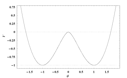
Figure 1: The field-theoretical potential (5) of the logarithmic BEC in the dimensionless units: $-\beta a^{3}$ (vertical axis) and $a^{-3/2}$ (horizontal axis).

For instance, as long as the potential (5) vanishes in the extrema $n_{\text{ext}}$, they describe the equilibrium configurations for “free” particles. These equilibria can be stable or unstable and here appears something which might look counterintuitive at first sight. The negative $\beta$ means that the the field-theoretical potential opens up and the above-mentioned extrema are minima but the energy functional is not bounded from below BialynickiBirula:1976zp , therefore, the stable equilibrium solution can only exist in a finite volume or in the additional external potential (“trap”) Guerrero2010 . On the contrary, when $\beta$ is positive then the potential (5) opens down but the energy functional is bounded from below. An apparent contradiction can be resolved if one recalls that we are dealing with the normalized wave-function and thus its square (the condensate density $n$) cannot grow arbitrarily large. The physical consequence is that the coherence length is always larger than the effective size of the droplet. In Sec. II and III we will show that this leads to one of the most important features of the Bose liquid with logarithmic nonlinearity: at positive $\beta$ it can be self-bound and stable (as to form the droplet-like object) even without any trapping potential.

Second, the logarithmic term in Eq. (2) can be associated with the certain kind of quantum-informational entropy $S_{\Psi}\propto-\int|\Psi|^{2}\ln{(\Xi|\Psi|^{2})}d^{3}x$, measuring the degree of quantum spreading of the BEC as a collective quantum object, as being described in the Appendix. The only difference from the interpretation presented there is that in the BEC case the logarithmic term describes the quantum information transfer between the states of the correlated particles which form the many-body state whereas the temperature $T_{\Psi}$ is a formal measure of the collisionless interactions inside the Bose liquid at zero (thermal) temperature, see the Appendix.

Third, using the Madelung representation of the wave function and the hydrodynamic form of the wave equation (2) pn66 ; Dalfovo:1999zz , the zero-temperature (collisionless) equation of state of the logarithmic BEC in the leading order with respect to the Planck constant is described by a kind of the Clapeyron-Mendeleev law,

$$p-p_{0}=-(m\beta)^{-1}n+{\cal O}(\hbar^{2})\propto T_{\Psi}n.$$ (6)

For comparison, the equation of state for the GP condensate would be $p\propto n^{2}$, thus, the logarithmic Bose liquid is more “ideal” than the Gross-Pitaevskii one yet non-trivial. From here it follows that the logarithmic BEC is the only one where the speed of sound (phonons) does not depend on the density in the leading order with respect to the Planck constant:

$$c_{s}=1/\sqrt{m|\beta|}+{\cal O}(\hbar).$$ (7)

Meanwhile, the speed of sound for the GP condensate scales as a square root of density. Due to this property the logarithmic BEC can be used to describe or mimic the induced relativity and several high-energy and gravitational phenomena, along the lines described in Refs. Zloshchastiev:2009aw ; Garay:1999sk ; Novello:2002qg , although considering these topics would bring us too far from the scope of the current paper.

Finally, in the GP case it is possible to differentiate between the “attractive” and “repulsive” interaction depending on a sign of the coupling constant. In our case the logarithm changes sign when density goes across the value $a^{-3}$ which results in changing the sign of the interaction in Eq. (2) and the type of the condensate depends not only on the sign of $\beta$ but also on whether the value of $na^{3}$ is smaller or larger than one.

II The logarithmic BEC in the empty space

While many of the properties discussed in this section hold also for the condensate in a trap, it is more clarifying to see them on the example of the released condensate. If it were the GP-type Bose gas then its properties would be nearly trivial: once the trap is off the GP condensate spreads uniformly all over the available space (if it is repulsive), or shrinks down until the new phase arises, in the case of attraction. The behavior of the free logarithmic BEC will be shown to be much more complex, mostly due to the properties of the logarithm mentioned above.

If we assume the isotropic case for simplicity and work in the center-of-mass reference frame of the condensate then $\Psi(\vec{x},t)=\Psi(|\vec{x}|)\exp{(-i\mu t/\hbar)}$, $\mu$ being the chemical potential, and the equation (2) reduces to the ordinary differential equation for the modulus of wave function $\Psi=\sqrt{n(r)}$ as the function of the radial coordinate only,

$$\frac{\hbar^{2}}{2m}\Delta\Psi+\left[\mu+\beta^{-1}\ln{(a^{3}\Psi^{2})}\right]\Psi=0,$$ (8)

where $\Delta\Psi=r^{-2}\partial_{r}(r^{2}\partial_{r}\Psi)$. Further it will be convenient to introduce a value of dimensionality of the length squared, $A_{\beta}=\hbar^{2}\beta/2m$ which measures the strength of the logarithmic interaction in terms of length scales, and a value of dimensionality of the energy, $E_{a}=\hbar^{2}/(2ma^{2})$ which is the de Broglie energy corresponding to the length scale $a$. Upon applying the normalization condition, $\int nd^{3}x=4\pi\int\limits_{0}^{\infty}\Psi^{2}r^{2}dr=N$, we deduce that the normalizable solution is only possible for positive $\beta$. The exact expressions for, respectively, the particle density and the chemical potential are:

$$n(r)=\Psi^{2}=n_{0}e^{-(r/a_{\beta})^{2}},$$ (9)

$$\mu=3\beta^{-1}\left[1-\ln{\left(\frac{N^{1/3}}{\sqrt{\pi}}\frac{a}{a_{\beta}}\right)}\right]=-\beta^{-1}\ln{\left(N/N_{0}\right)},$$ (10)

where $n_{0}=N/(\pi^{3/2}a_{\beta}^{3})=(e/a)^{3}N/N_{0}$, $a_{\beta}=\sqrt{A_{\beta}}=\hbar\sqrt{\beta/2m}$, and $N_{0}\equiv(e\sqrt{\pi}a_{\beta}/a)^{3}$ is the number of particles at which the chemical potential changes its sign. The energy functional for the logarithmic BEC can be defined in a standard way (see, e.g., Sec 6.1 of the book pethick04 ):

$$E[n]=4\pi\int\limits_{0}^{\infty}\left\{\frac{\hbar^{2}}{2mn}(\vec{\nabla}\sqrt{n})^{2}-\beta^{-1}\left[\ln{(na^{3})}-1\right]\right\}nr^{2}dr,$$ (11)

which yields the expression for the energy per particle:

$$E/N=3\beta^{-1}\left[\frac{4}{3}-\ln{\left(\frac{N^{1/3}}{\sqrt{\pi}}\frac{a}{a_{\beta}}\right)}\right]=\beta^{-1}\left[1-\ln{\left(N/N_{0}\right)}\right].$$ (12)

One can see that $E$ as a function of $N$ vanishes in the origin and at $eN_{0}$, and has a positive-valued local maximum, i.e., it is bounded from above (see Fig. 2)

$$E/N\leqslant\beta^{-1},$$ (13)

where the value of $N$ at which the maximum occurs is given by the transcendental equation $\ln{\left(N/N_{0}\right)}+N_{0}/N=1$. Notice that for the non-negative values of $E$ there exists some sort of degeneracy - one value of energy corresponds to two values of $N$. This will be discussed below in more detail. Further, if we treat $E$ as a function of the coupling then it obviously vanishes when $\beta^{-1}$ approaches zero. However, it can also vanish at the nonzero value of the coupling which can be made obvious by rewriting the expression as

$$E/N=-\frac{3}{2}\beta^{-1}\ln{\left(\beta^{-1}/\beta_{0}^{-1}\right)},$$ (14)

where $\beta_{0}^{-1}\equiv\pi e^{8/3}N^{-2/3}E_{a}$ represents the non-zero value of the parameter $\beta$ at which this energy vanishes. From this expression one can also see that the energy is bounded from above

$$E(\beta)\leqslant\frac{3}{2}e^{-1}N\beta_{0}^{-1}=\frac{3}{2}\pi e^{5/3}N^{1/3}E_{a},$$ (15)

with this local maximum occurring at $\beta_{\text{max}}^{-1}=\beta_{0}^{-1}/e=\pi e^{5/3}N^{-2/3}E_{a}$.

It is important to note that both the chemical potential (10) and the ground-state energy (12) depend on the parameter $a$ as $\ln{a_{\beta}/a}$ and as we show below this term can only be positive as $a_{\beta}>a$.

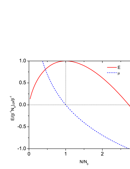
Figure 2: The total energy (solid line) and the chemical potential (dotted line) for the logarithmic BEC with positive $\beta$ in absence of any trap as a function of the number of particles.

II.1 Effective potential, stability and critical mass

For the analysis of the solutions of the generic equation of the form

$$\left[-\frac{\hbar^{2}}{2m}\vec{\nabla}^{2}+V_{\text{ext}}(\vec{x},\,t)+F(|\Psi|^{2})-\mu\right]\Psi=0$$

it is often convenient to introduce the notion of the effective potential $V_{\text{eff}}(r)\equiv V_{\text{ext}}(\vec{x},\,t)+F(|\Psi(r)|^{2})$ which in our case is defined as

$$V_{\text{eff}}(r)\equiv-\beta^{-1}\ln{(a^{3}\Psi^{2}(r))}.$$ (16)

Being evaluated on the solution (9) it becomes the quadratic function of radius-vector:

$$V_{\text{eff}}(r)=\frac{1}{2}m\omega_{\text{eff}}^{2}r^{2}+\mu-\frac{3}{2}\hbar\omega_{\text{eff}},$$ (17)

where

$$\omega_{\text{eff}}=2\beta^{-1}/\hbar.$$ (18)

Therefore, the effect from the logarithmic term here is that it effectively introduces the trap with the frequency which is controlled by $\beta$ whereas the system can be viewed as a particle of energy $\mu$ whose center of mass is located in this trap. Then the stability of the solution against a small perturbation is ensured by the fact that this frequency is non-negative if $\beta$ is non-negative.

This is also confirmed by the Vakhitov-Kolokolov stability criterion vk73 which in our case is equivalent to the non-positivity of the derivative of the chemical potential with respect to $N$. From Eq. (10) one can derive that this derivative equals to $-\beta^{-1}/N$ and thus it is non-positive indeed.

There is, however, an additional issue of stability. From Eqs. (12) or (14) it is clear that for the non-negative values of $E$ there exists some sort of degeneracy - one value of energy is achieved at two values of $N$ or $\beta$, respectively. This indicates that the system spontaneously ‘chooses” either of these values at no cost of binding energy, and the so-called mechanical instability occurs hs96 . Thus, our condensate is impeccably stable only at

$$E<0,$$ (19)

which means that the number $N$ must be bounded from below

$$N>N_{\text{min}}\equiv eN_{0}.$$ (20)

The physical meaning of the latter is that one cannot create the stable logarithmic condensate with just any amount of initial (bare) particles - it must be larger than the value $N_{\text{min}}$. In other words, in the presence of certain long-range correlations and multi-body scattering the initial Bose system must have the mass larger than the critical one, $mN_{\text{min}}$, for the Bose condensation to happen.

II.2 Self-sustainability and droplet formation

An important thing to notice is that indeed the density of the free condensate with the positive $\beta$ does not become the uniform one - in empty space the condensate rather tends to take the shape of a spherical Gaussian droplet, with a characteristic size of order $a_{\beta}$. Our droplet, however, is different from the ordinary ones. As long as its density $n(r)$ is described by the Gaussian the major portion of mass and energy is localized in a finite volume $\tfrac{1}{6}\pi a_{\beta}^{3}$ - similarly to the liquid droplets in the classical world. The difference is that the Gaussian vanishes at the infinity only, therefore, our droplet is essentially inhomogeneous and has no sharply defined external surface, hence, its stability is ensured by the nonlinear quantum effects in the bulk rather than by the surface tension.

Further, from Eqs. (10) and (12) it follows that for the Gaussian solution the following relation holds

$$\mu-E/N=-\beta^{-1},$$ (21)

which essentially means that the chemical potential counted from the energy per particle is negative in our case. A similar feature was observed in real superfluids, such as ⁴He woo76 , therefore, models involving the logarithmic nonlinearity might find an application there.

II.3 Quantum Shannon entropy and non-thermal temperature

Let us consider now the notion of the information entropy introduced in the Appendix. In the context of the Bose-condensation phenomenon the entropy $S_{\Psi}$ is a measure of information stored in the microscopical configuration of $N$ bosons which form the droplet where the square of wave function determines the density value and constant $\Xi$ defines the information entropy reference frame. Besides, $S_{\Psi}$ becomes a thermodynamic-like measure of the quantum spreading of the droplet as a whole.

To start with $S_{\Psi}$, it is natural to measure the constant $\Xi$ in the units of $a^{3}$: $\Xi\equiv Z_{0}^{1/N}a^{3},$ where $Z_{0}$ is a dimensionless constant. Then the entropy (74) can be written as

$$k_{B}^{-1}S_{\Psi}=k_{B}^{-1}S_{\Psi}^{(0)}+\int n\ln{(a^{3}n)}d^{3}x,$$ (22)

where $S_{\Psi}^{(0)}\equiv k_{B}\ln{Z_{0}}$ is the reference entropy. One can physically justify the identification of an entropy using the fact that the energy functional is bounded from below. The reasoning is the following. The energy needed to cut the $N$-particle droplet into two equal parts is $\Delta E=-N\beta^{-1}\ln 2$, into three parts it is $\Delta E=-N\beta^{-1}\ln 3$ and so on. Therefore, the maximum binding energy which is saved in a droplet and can be realized is no more than $\Delta Q=N\beta^{-1}\ln N$. So we can use the thermodynamic definition of entropy through $\Delta Q=T_{\Psi}\Delta S_{\Psi}$. The parts of the energy (12) which are proportional to $N$ do not contribute to $\Delta E$ and can be taken either to $E^{(0)}$ or to $S_{\Psi}^{(0)}$ while $S_{\Psi}\propto N\ln{N}$:

$$E=E^{(0)}-T_{\Psi}S_{\Psi},$$ (23)

$$S_{\Psi}=k_{B}N\ln{N},$$ (24)

$$E^{(0)}=N\beta^{-1}(1+\ln{N_{0}}),$$ (25)

where $T_{\Psi}=(k_{B}\beta)^{-1}$ is the associated temperature. Thus, we can formally divide the energy into two types - into the entropy and the part which is linear w.r.t. $N$. Therefore, the latter is linear w.r.t. density too, while $E^{(0)}/N$ can be considered as the energy of a free quasi-particle. Alternatively, the $N$-linear part can be considered as a reference entropy $S_{\Psi}^{(0)}=N(1+\ln{N_{0}})$ which is supposed to be positive.

In general, such definition of entropy can be deduced for any shape of the logarithmic BEC (e.g., in the trap) as the integral in Eq. (22) can be always presented in the form $N\ln{N}+Nf$ where $f$ is an $N$-independent function of the parameters of a system. If we require the positiveness of the additive part of the energy (it means that $f$ is always positive) the entropy part of the energy Eq. (23) determines its lower limit at given $N$.

II.4 Emergent spatial extent

From Eq. (9) one can see that while the logarithmic condensate is “made” of $N$ bare particles which are assumed to be point-like the resulting Gaussian droplet acquires a finite size $a_{\beta}$. Besides, it is clear that the particle density of the logarithmic condensate is bounded from above, $n\leqslant n_{0}$ , which implies that the average volume occupied by a condensate’s quasi-particle is bounded from below

$$\langle\text{Vol}\rangle\geqslant(\sqrt{\pi}a_{\beta})^{3}/N.$$ (26)

Together with the arguments coming from the analysis of elementary excitations, see the paragraph after Eq. (55), this means that the effective size of the quasi-particle can be non-zero at the non-zero $\beta^{-1}$. Recalling the meaning of $a_{\beta}$ as an effective size of the Gaussian droplet, we see that the latter can accommodate no more than $\tilde{N}_{\text{max}}$ quasi-particles, i.e.,

$$\tilde{N}\leqslant\tilde{N}_{\text{max}}\approx\tfrac{1}{6}\pi a_{\beta}^{3}/\langle\text{Vol}\rangle=N/(6\sqrt{\pi}),$$ (27)

where tilded values refer to the condensate’s quasi-particle modes.

However, the inequalities of this type are trivial in a sense; they follow entirely from the normalization condition and thus they are not necessary specific of the logarithmic model. In our case, the better bound can be derived from physical arguments. It is clear that the $N$-linear part (25) must be non-negative because this energy can only increase when $N$ does. Thus, we have to impose $\ln{N_{0}}\geqslant-1$ which is equivalent to $n_{0}a^{3}\leqslant e^{4}N$ or $a_{\beta}\geqslant a/(\pi^{3/2}e^{4/3})$ (we remind that $a_{\beta}$ is the mean size of the Gaussian droplet). As long as $n\leqslant n_{0}$, we obtain

$$na^{3}\leqslant n_{0}a^{3}\leqslant Ne^{4},$$ (28)

which implies that $a_{r}/r\leqslant 1$, where $a_{r}=a/(Ne^{4})^{1/3}$ is the quasi-particle effective size and $r$ is the mean interparticle distance. Thus, the smallest volume of the system of $N$ particles is nonzero but of the order $a^{3}$. This is crucially different from what the GP approach would yield - there no such effect appears, the Gaussian-type droplet can only form when the gas is placed into the external trapping potential of a special kind. It is interesting that the spatial extent exists in the worldvolume-formulated theories Green:1987sp (where it is postulated from the beginning), and also it is known to arise as the quantum effect in the quantum mechanics of point particles on non-commutative spaces Rohwer:2010zq . In our case, however, no spatial extent was initially postulated (the bare particles were assumed to be point-like, according to the standard quantum-mechanical approach) and no quantum commutation rules were modified - instead, the non-zero size is an emergent quantum phenomenon due to the peculiar type of correlations between particles’ wave-functions.

II.5 Effective potential and finite volume

As shown above, the value $a^{3}$ is the smallest possible volume of the system of $N$ particles whereas $a_{r}\sim a/N^{1/3}$ is the size of a quasi-particle (for brevity, in this section we neglect the ${\cal O}(1)$ factors such as those containing $e$ and $\pi$). One can argue that the condition (28) means that states with $na^{3}>N$ can not be physically reached as particles commence to “overlap” each other. Therefore, the effective potential,

$$V(n)\equiv V_{\beta}-\mu n,$$ (29)

is confined to the given bounds, see Fig. 3. In particular, it is naturally bounded from below because $na^{3}\ln{(na^{3})}\ll N\ln{N}$. A similar condition holds for the central density which implies that $a_{\beta}/a>1$ (the droplet’s volume must not be smaller than the smallest one). Therefore, our potential for the positive $\beta$ has two minima, one being located at zero, and the other being at the limit value corresponding to maximally dense packing. The latter is usually deeper and hence defines the ground state. For the system with a finite number of particles, such as our droplet, the density of a dense packing is much larger than its central density $n_{0}$. The depth of this minimum can be controlled with a quadratic term, see Fig. 3. If one considers this potential with the extra quadratic (chemical potential) term one can find that negative chemical potentials shift the local maximum to the large values. At $\ln{(na^{3})}=1-\mu_{max}/\beta^{-1}$ the minimum at zero becomes deeper and the maximally dense packing state is not the ground state anymore hence the system can not be self-sustained anymore.

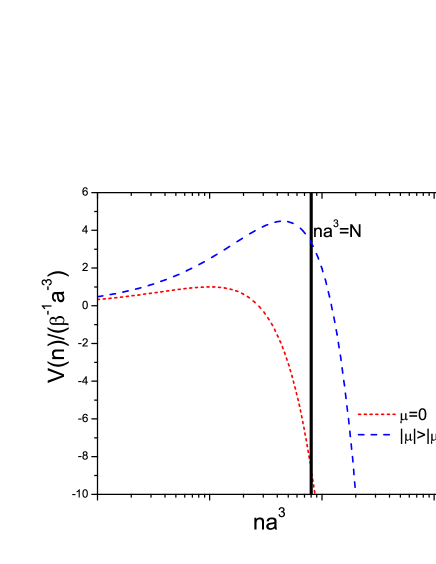
Figure 3: The effective potential (29) for the logarithmic BEC for zero and large negative chemical potentials

The size of the droplet is defined by a parameter $\beta$ and by putting more and more particles into the system the maximum density can be reached when $na^{3}\approx N$ which means $a_{\beta}\approx a$. One might expect that at a given $N$ one can get a denser condensate by putting it inside a trap, but the size of this trap should be smaller than $a_{\beta}$. In this case the zero minimum of the effective potential is responsible for the ground state. It should be noted here that if one selects the harmonic trap to identify such a phase transition it might be rather difficult as the ground state for both phases is still described by the Gaussian functions, only of a different width. A clearer way would be to use a non-harmonic trap so that a phase transition should reveal itself through the change in the shape of the droplet.

As for the case of the negative $\beta$, the ground state is determined there by the minimum of the effective potential at $na^{3}=1$. We found that this state can not be self-bound and can be confined only in a trap.

III Logarithmic BEC in a trap

First we consider the logarithmic BEC placed in the infinite-walled spherical square-well potential of radius $d$. As one can see from (31), the condensate density in a trap can be much larger than for a free droplet, see Fig. 4 for the case of positive $\beta$. When the size of trap $d$ is much larger than the characteristic size of the droplet $a_{\beta}$, the condensate does not “sense” the trap and behaves like a self-bounded Gaussian droplet. As long as $d\sim a_{\beta}$ the condensate begins loosing its Gaussian shape and becomes denser in the center. In the case of the negative $\beta$ there is no localized solution and condensate tends to fill the whole trap of any size. It should be noted that the condensate density profile does not depend on the quasi-particle’s size and only determines the possible number of particles in the condensate.

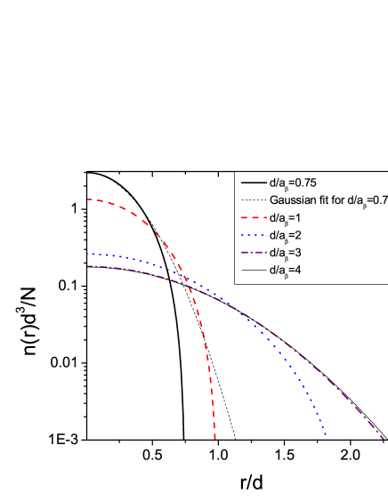
Figure 4: The density of the logarithmic BEC in the infinite-walled spherical well of radius $d$.

Now, let us place the logarithmic condensate into the isotropic harmonic trap of frequency $\omega$. Then the equation (2) reduces to the following one

$$-\frac{\hbar^{2}}{2m}\Delta\Psi+\left[\tfrac{1}{2}m\omega^{2}r^{2}-\mu-\beta^{-1}\ln{(a^{3}\Psi^{2})}\right]\Psi=0,$$ (30)

where $a_{\omega}=\sqrt{\hbar/m\omega}$ is the characteristic width of the harmonic trap. Unlike the previous (free) case, the exact normalized solution of this equation exists both for positive and negative $\beta$’s and still has the Gaussian form:

$$n(r)=n_{0}(\omega)e^{-(r/a_{\beta\omega})^{2}},$$ (31)

where

$$n_{0}(\omega)\equiv\pi^{-3/2}N/a_{\beta\omega}^{3},\quad a_{\beta\omega}\equiv\sqrt{\frac{2A_{\beta}}{1-\chi}}=\frac{\hbar}{\sqrt{m\epsilon_{\omega\beta}}},$$ (32)

and

$$\chi\equiv-\,\text{sign}\left(\beta\right)\sqrt{1+(2A_{\beta}/a_{\omega}^{2})^{2}}=-\,\text{sign}\left(\beta\right)\sqrt{1+(\hbar\omega\beta)^{2}},$$ (33)

so that the values $\epsilon_{\omega\beta}=(1-\chi)/\beta$ and $\sigma$ are never negative. The normalization condition yields the allowed value of the chemical potential:

$$\mu_{\omega}=\frac{3}{2}\beta^{-1}\left[1-\chi-\ln{\left(\frac{ma^{2}N^{2/3}}{\pi\hbar^{2}}\frac{1-\chi}{\beta}\right)}\right]=-\beta^{-1}\ln{\left(N/N_{0}(\omega)\right)},$$ (34)

where

$$N_{0}(\omega)\equiv\pi^{3/2}\left(a_{\beta\omega}/a\right)^{3}e^{\frac{3}{2}(1-\chi)},$$ (35)

and in the limit $\omega\to 0$ at the positive $\beta$ the expressions expectedly reduce to those from the previous section, $N_{0}(\omega=0)=N_{0}$.

By analogy with the spherical-wall case one can show that when $\hbar\omega\gg\beta^{-1}$ (which is equivalent to $a_{\omega}<a_{\beta}$) the central density in the trap can be considerably larger than the central density of the droplet. But of course it can not be infinitely large because the condensate density has an upper bound (28).

Further, the energy of the system is given by

$$E[n]=4\pi\int\limits_{0}^{\infty}\left\{\frac{\hbar^{2}}{2mn}(\vec{\nabla}\sqrt{n})^{2}+\frac{1}{2}m\omega^{2}r^{2}-\beta^{-1}\left[\ln{(na^{3})}-1\right]\right\}nr^{2}dr,$$ (36)

hence the energy per particle becomes

$$E_{\omega}/N=\frac{3}{2}\beta^{-1}\left[\frac{5}{3}-\chi-\ln{\left(\frac{ma^{2}N^{2/3}}{\pi\hbar^{2}}\frac{1-\chi}{\beta}\right)}\right]=\beta^{-1}\left[1-\ln{\left(N/N_{0}(\omega)\right)}\right].$$ (37)

The relation $\mu_{\omega}-E_{\omega}/N=-\beta^{-1}$ holds, similarly to the case of the condensate without a trap, which means that the chemical potential counted from the condensate energy per particle is negative (positive) for the positive (negative) $\beta$. The plot of the energy in $\beta^{-1}N_{0}$ units for the logarithmic BEC in an isotropic harmonic trap as functions of a number of particles in $N_{0}$ units is given in Fig. 5.

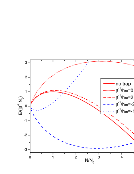
Figure 5: The energy of the logarithmic BEC in an isotropic harmonic trap versus the number of particles for different values of $\beta^{-1}/\hbar\omega$.

III.1 Effective potential and linear stability

The effective potential in this case is defined as

$$V_{\text{eff}}(r)\equiv\frac{1}{2}m\omega^{2}r^{2}-\beta^{-1}\ln{(a^{3}\Psi^{2}(r))}.$$ (38)

Being evaluated on the solution (31) it becomes:

$$V_{\text{eff}}(r)=\frac{1}{2}m\omega_{\text{eff}}^{2}r^{2}+\mu_{\omega}-\frac{3}{2}\hbar\omega_{\text{eff}},$$ (39)

where

$$\omega_{\text{eff}}=\epsilon_{\omega\beta}/\hbar=\beta^{-1}\left(1+\,\text{sign}\left(\beta\right)\sqrt{1+(\hbar\omega\beta)^{2}}\right)/\hbar.$$ (40)

Therefore, the effect from the logarithmic term here is that it replaces the trap frequency with the modified one which depends on $\beta$ and it is always non-negative regardless of the signs of $\omega$ or $\beta$. Thus, the coefficient at $r^{2}$ is non-negative regardless of the sign of $\beta$ either, hence, the Gaussian solution (31) is stable both at a positive and negative $\beta$. Moreover, it stays stable at arbitrary small $\hbar\omega\beta$ unless the latter vanishes exactly - then the negative-$\beta$ solution decays, in agreement with the result from the previous section. This feature shows another difference of the logarithmic BEC from the GP one - the latter decays when the non-linear coupling (proportional to the scattering length) becomes negative. These properties are essentially rooted in the sign-changing property of the logarithm discussed in the introductory part of the paper.

III.2 Mechanical stability and related bounds

As for the mechanical stability the arguments given for the no-trap case can be easily generalized for our case: for the logarithmic condensate to be stable in a harmonic trap the following inequality must hold

$$\beta^{-1}\left[1-\ln{\left(N/N_{0}(\omega)\right)}\right]<0,$$ (41)

whose physical implications are to be discussed now.

As long as the coupling is not necessarily positive now we must distinguish two cases:

(a) Positive $\beta$. The inequality (41) brings, as in the no-trap case, the lower bound for the number of condensate particles, with the only difference that now it becomes $\omega$-dependent

$$N>N^{(+)}=eN_{0}(\omega)=\pi^{3/2}\left(\frac{a_{\beta\omega}}{a}\right)^{3}e^{\tfrac{1}{2}(3|\chi|+5)}$$

$$\qquad=\left(\frac{2\pi}{|\chi|+1}\right)^{3/2}\left(\frac{a_{\beta}}{a}\right)^{3}e^{\tfrac{1}{2}(3|\chi|+5)},$$ (42)

so it can be regulated by adjusting the trap’s frequency. Similarly to the no-trap case, this bound implies that one can not create the logarithmic condensate with just any amount of initial (bare) particles - it must be larger than the critical value $N^{(+)}$ which is frequency-dependent now. If the frequency energy is much smaller than the logarithmic coupling, $\hbar\omega\ll\beta^{-1}$, then the critical value is a quadratic function of the frequency:

$$N^{(+)}=eN_{0}\left[1+\frac{3}{8}(\hbar\omega\beta)^{2}\right]+{\cal O}\left((\hbar\omega\beta)^{4}\right),$$ (43)

where $N_{0}$ was defined in the no-trap case. If the frequency energy is much larger than the logarithmic coupling, $\hbar\omega\gg\beta^{-1}$, then the critical value grows exponentially with an increasing frequency:

$$N^{(+)}\approx\pi^{3/2}(a_{\omega}/a)^{3}\exp{\left(\tfrac{3}{2}\hbar\omega\beta\right)},$$ (44)

which means that the trapping potential dominates over the logarithmic term in the wave equation, and the condensate goes into another phase.

(b) Negative $\beta$. There appears the upper bound for the number of condensate particles which is also $\omega$-dependent

$$N<N^{(-)}=eN_{0}(\omega)=\pi^{3/2}\left(\frac{a_{\beta\omega}}{a}\right)^{3}e^{-\tfrac{1}{2}(3|\chi|-5)}$$

$$\qquad=\left(\frac{2\pi}{|\chi|-1}\right)^{3/2}\left(\frac{\sqrt{|A_{\beta}|}}{a}\right)^{3}e^{-\tfrac{1}{2}(3|\chi|-5)}.$$ (45)

This critical value can be also regulated by the trap’s frequency. If the frequency energy is much smaller than the logarithmic coupling, $\hbar\omega\ll\beta^{-1}$, then the critical value scales as the inverse cube of the frequency:

$$N^{(-)}\approx e\pi^{3/2}(a_{\beta\omega m}/a)^{3},$$ (46)

where $a_{\beta\omega m}\equiv a_{\omega}^{2}/\sqrt{|A_{\beta}|}=\omega^{-1}\sqrt{\frac{2}{m|\beta|}}$ is another length scale. When the frequency vanishes, $N^{(-)}$ diverges which indicates that at negative $\beta$ there is no Gaussian solution for the logarithmic condensate in empty space, as was mentioned in the previous section. If the frequency energy is much larger than the logarithmic coupling, $\hbar\omega\gg\beta^{-1}$, then the critical value vanishes exponentially with increasing frequency:

$$N^{(-)}\approx\pi^{3/2}(a_{\omega}/a)^{3}\exp{\left(-\tfrac{3}{2}\hbar\omega|\beta|\right)},$$ (47)

as the trapping potential dumps the logarithmic-term effects and thus destroys the logarithmic condensate.

IV Excitations in the logarithmic BEC

Small fluctuations in quantum Bose liquids can be conditionally cast into two classes - collective modes and elementary excitations. The former describe the motion of the liquid or a large part thereof as a whole, the latter are localized and can be viewed as particle-like objects. Although, due to the particle-wave duality there is no exact border between these classes: for instance, a phonon which is a quantum of collective vibrational modes can be also described as an elementary excitation via the Bogoliubov approach.

The collective mode of the logarithmic BEC is governed by the second-rank tensor (“acoustic metric”) corresponding to the conformally-flat Lorentzian manifold Zloshchastiev:2009aw . That result can be easily transferred to the condensed matter physics provided that the fundamental velocity constant is assumed to be the speed of sound. Here we consider the other class, elementary excitations, for the logarithmic condensate in the empty space. To this effect we perform the second quantization by going from the wave-functions $\Psi$ to the field operators via the Bogoliubov decomposition

$$\Psi\to\hat{\Psi}=\sqrt{n_{0}}+\delta\hat{\Psi},$$ (48)

where $n_{0}$ is the density of the condensate (for simplicity we assume the latter being uniform which is a valid approximation at the length scales are smaller compared with the size of the droplet), $\delta\hat{\Psi}$ is the operator of excitations, $[\delta\hat{\Psi},\delta\hat{\Psi}^{\dagger}]=\theta$, and throughout the paper the non-polynomial functions of operators are defined as the Taylor series of matrices, as usual. One of the simplest forms of the Hamiltonian can be easily deduced from Eq. (1) assuming the normal-ordering approximation

$$\hat{H}=\int d{\bf r}\left[-\hat{\Psi}^{\dagger}\frac{\hbar^{2}}{2m}\Delta\hat{\Psi}-\beta^{-1}:\hat{\Psi}^{\dagger}\hat{\Psi}\ln{(a^{3}\hat{\Psi}^{\dagger}\hat{\Psi})}:\right],$$ (49)

where the colon means the normal ordering of the operators. Upon applying the Bogoliubov decomposition, we obtain

$$\hat{H}-\mu\hat{N}=\left[\epsilon_{0}-\beta^{-1}\left(1+\ln{(a^{3}n_{0})}\right)\right]\delta\hat{\Psi}^{\dagger}\delta\hat{\Psi}$$

$$\qquad\qquad\quad-\frac{\beta^{-1}}{2}\left(\delta\hat{\Psi}^{2}+\delta\hat{\Psi}^{\dagger 2}\right),$$ (50)

when omitting non-quadratic terms; here we denote $\epsilon_{0}\equiv p^{2}/2m-\mu$, $p$ being the absolute value of the momentum vector. Upon applying the Bogoliubov diagonalization procedure we obtain

$$\hat{H}-\mu\hat{N}=\epsilon\hat{b}^{\dagger}b,$$ (51)

$$\epsilon^{2}\equiv\left[\epsilon_{0}-\beta^{-1}\left(1+\ln{(a^{3}n_{0})}\right)\right]^{2}-\beta^{-2},$$ (52)

where $\hat{b}^{\dagger}$ and $\hat{b}$ are the creation and annihilation operators of the quasi-particles with momenta p, $[\hat{b},\hat{b}^{\dagger}]=[\delta\hat{\Psi},\delta\hat{\Psi}^{\dagger}]$, defined as the linear combinations

$$\delta\hat{\Psi}=\kappa\hat{b}+\sqrt{\kappa^{2}-1}\,\hat{b}^{\dagger},$$

$$\delta\hat{\Psi}^{\dagger}=\sqrt{\kappa^{2}-1}\,\hat{b}+\kappa\hat{b}^{\dagger},$$

where

$$\kappa\equiv-\frac{\kappa_{2}}{\sqrt{2}}\left(\kappa_{1}^{2}-\kappa_{2}^{2}\right)^{-1/4}\left(\kappa_{1}-\sqrt{\kappa_{1}^{2}-\kappa_{2}^{2}}\right)^{-1/2},$$

$$\kappa_{1}\equiv\epsilon_{0}-\beta^{-1}\left(1+\ln{(a^{3}n_{0})}\right),$$

$$\kappa_{2}\equiv\beta^{-1},$$

and we can write the dispersion relation for the excitations of the logarithmic BEC in the form

$$\epsilon(p)=\sqrt{\left[\frac{p^{2}}{2m}-\mu-\beta^{-1}\left(1+\ln{(a^{3}n_{0})}\right)\right]^{2}-\beta^{-2}},$$ (53)

and also we assume $\beta$ to be positive for the remainder of this section, therefore, the value of the chemical potential can be borrowed from Eq. (10). As compared with the dispersion relation for the excitations in the GP condensate pethick04 ,

$$\epsilon_{\text{GP}}(p)=\sqrt{\frac{p^{2}}{2m}\left(\frac{p^{2}}{2m}+2n_{0}U_{0}\right)},$$

the dispersion for the logarithmic Bose liquid has a number of drastic differences.

The first thing to notice is that the requirement of non-negative energy points out the existence of the forbidden region of momenta (where $\epsilon$ becomes negative or even complex which indicates instability issues). The forbidden momenta region is given by the inequality (we are neglecting the chemical potential for the moment)

$$\beta^{-1}\ln{(a^{3}n_{0})}\leqslant\left(\frac{p^{2}}{2m}\right)_{\text{forbid}}\leqslant\beta^{-1}\left[\ln{(a^{3}n_{0})}+2\right]\quad \quad\ln{(a^{3}n_{0})}>0,$$ if (54)

$$0\leqslant\left(\frac{p^{2}}{2m}\right)_{\text{forbid}}\leqslant\beta^{-1}\left[\ln{(a^{3}n_{0})}+2\right]\quad \quad\ln{(a^{3}n_{0})}\leqslant 0,$$ if (55)

and this region only exists if the upper bound $\ln{(a^{3}n_{0})}+2$ is positive-valued. The latter condition is equivalent to $r_{0}/e^{2/3}>a$ where $r_{0}=n_{0}^{-1/3}$ is the average spacing between quasi-particles. Therefore, the appearance of the gap in the momentum space is in fact another manifestation of the emergent spatial extent phenomenon discussed above.

Thus, depending on the value of the background condensate density the momentum space of the model can contain forbidden regions and thus can have a non-trivial topology. To see the full picture, we introduce two auxiliary values of dimensionality energy

$$\epsilon_{1}\equiv\beta^{-1}\ln{(a^{3}n_{0})}+\mu,$$ (56)

$$\epsilon_{2}\equiv\epsilon_{1}+2\beta^{-1}>\epsilon_{1},$$ (57)

then the dispersion relation (53) can be rewritten in the form

$$\epsilon(p)=\sqrt{\left(\frac{p^{2}}{2m}-\epsilon_{1}\right)\left(\frac{p^{2}}{2m}-\epsilon_{2}\right)},$$ (58)

which is more convenient when classifying dispersion relations according to the topology of the momentum space. We distinguish the following cases:

(i) $\epsilon_{2}<0$. Then $\epsilon_{1}$ must be negative as well, therefore, energy vanishes nowhere and the topological structure of the momentum space is trivial. The quasiparticle’s spectrum is fully gapped and equivalent to that of the massive relativistic particle moving in the 4D spacetime with the fundamental velocity constant determined by the speed of sound $\bar{c}$:

$$\epsilon=\sqrt{p^{2}\bar{c}^{2}+m_{\star}^{2}\bar{c}^{4}}+{\cal O}(p^{4}/m^{2})=\Delta+\frac{p^{2}}{2m_{\star}}+{\cal O}(p^{4}/m^{2}),$$ (59)

where

$$\Delta=\sqrt{\epsilon_{1}\epsilon_{2}},\ \ m_{\star}=-\frac{2\Delta}{\epsilon_{1}+\epsilon_{2}}m,$$

$$\bar{c}=\sqrt{-\frac{\epsilon_{1}+\epsilon_{2}}{2m}}=\sqrt{\frac{\beta^{-1}-\epsilon_{2}}{m}}.$$ (60)

To allow the excitations of this type, the background condensate density must be below the first threshold value

$$n_{0}<n_{T},$$ (61)

where

$$n_{T}\equiv a^{-3}e^{-\mu\beta-2}=\frac{1}{e^{2}a^{3}}\frac{N}{N_{0}}=\frac{N}{e^{5}\pi^{3/2}a_{\beta}^{3}}.$$ (62)

(ii) $\epsilon_{2}=0$. Then $\epsilon_{1}=-2\beta^{-1}$ and thus it is still negative, in the momentum space there appears a zero-energy point, at $p=0$, so the topological structure is still trivial and this case can be treated as a limit of the previous one. The quasi-particle’s spectrum in the vicinity of this point is equivalent to that of a phonon or a massless relativistic particle moving in a spacetime with the fundamental velocity constant $c_{0}$:

$$\epsilon^{2}=c_{0}^{2}p^{2}+{\cal O}(p^{4}),$$ (63)

where the speed of sound is given by

$$c_{0}\equiv 1/\sqrt{m\beta},$$ (64)

so that $c_{0}=c_{s}$, cf. Eq. (7). To allow the excitations of this type, the background condensate density must be equal to the first threshold

$$n_{0}=n_{T}.$$ (65)

(iii) $\epsilon_{2}>0$, $\epsilon_{1}<0$. To allow the excitations of this type, the background condensate density must lie between the first and second threshold values

$$n_{T}<n_{0}<e^{2}n_{T},$$ (66)

then in the momentum space there appears a zero-energy sphere of radius $p=\sqrt{2m\epsilon_{2}}$. The positive-energy modes are only located outside it, the quasiparticle’s spectrum in the vicinity of this sphere is equivalent to that of a tachyonic particle moving in a spacetime with the fundamental velocity constant $c_{2}$:

$$\epsilon^{2}=p^{2}c_{2}^{2}+m_{2}^{2}c_{2}^{4}+{\cal O}\left((p^{2}-2m\epsilon_{2})^{2}\right),$$ (67)

where the speed of sound and imaginary mass are

$$c_{2}=\sqrt{\frac{\epsilon_{2}-\epsilon_{1}}{2m}},\ \ m_{2}=2i\sqrt{\frac{\epsilon_{2}}{\epsilon_{2}-\epsilon_{1}}}m.$$ (68)

In particle physics such models are usually rejected as incompatible with Lorentz symmetry but in our case this can not be a valid reason: this symmetry is not a fundamental but rather an emergent phenomenon which appears at the lowest levels of energy.

(iv) $\epsilon_{2}>0$, $\epsilon_{1}=0$. This happens when the background density approaches the second threshold

$$n_{0}=e^{2}n_{T},$$ (69)

then in the momentum space there appears the zero-energy sphere of radius $p=\sqrt{2m\epsilon_{2}}$ and the zero-energy point at $p=0$. This leads to degeneracy and the appearance of two zero-energy states. The first mode is identical to the mode described in the previous item upon setting $\epsilon_{1}$ to zero. The other mode, the one with vanishing $p$, has the formal dispersion relation:

$$\epsilon^{2}=-\frac{\epsilon_{2}}{2m}p^{2}+{\cal O}\left(p^{4}\right),$$ (70)

which is of the quaternionic or 4D Euclidean ($SO(4)$-symmetric) type. However, this dispersion is only valid at $p=0$, therefore, this mode is non-propagating.

(v) $\epsilon_{2}>0$, $\epsilon_{1}>0$. This corresponds to the density growing above the second threshold

$$n_{0}>e^{2}n_{T},$$ (71)

then the momentum space gets split by two zero-energy spheres, of radii $\sqrt{2m\epsilon_{1}}$ and $\sqrt{2m\epsilon_{2}}$, which leads to degeneracy and the appearance of two zero modes. Positive-energy modes form two bands, $p<\sqrt{2m\epsilon_{1}}$ and $p>\sqrt{2m\epsilon_{2}}$. The first zero mode, located near the internal sphere $\sqrt{2m\epsilon_{1}}$, is described by the dispersion:

$$\epsilon^{2}=\frac{\epsilon_{1}-\epsilon_{2}}{m}p^{2}+2\epsilon_{1}(\epsilon_{2}-\epsilon_{1})+{\cal O}\left((p^{2}-2m\epsilon_{1})^{2}\right),$$ (72)

so it belongs to the above-mentioned quaternionic type with the only difference that now its energy is positive and the momentum does not vanish. The other zero-energy mode is of the tachyonic type, it is equivalent to the one described by Eq. (67).

To conclude, the topology of the momentum space of the logarithmic BEC excitations depends on the background value of the condensate’s density. In its turn, depending on the topology of the momentum space their dispersion relations can cover all cases described by the symmetries of the special orthogonal groups of order four - massive relativistic, massless relativistic, tachyonic and quaternionic. The tachyonic (quaternionic) mode arises when the momentum space contains the zero-energy sphere so that positive-energy states are located outside (inside) it. One can also notice that the dispersion relations become more and more exotic as the background density grows. This is in fact another manifestation of the above-mentioned emergent size effect.

V Conclusion

In this paper we considered the toy model based on the logarithmic Schrödinger equation and applied it to describing the ground state and excitations of some hypothetical Bose condensate. That is why we did not specify why and how such sort of nonlinearity might exist in real Bose liquids. We only pointed out that LogSE, despite its simplicity, reveals an interesting class of solutions and it can possibly be adapted for a description of strongly- interacting Bose liquids. The important feature of the logarithmic BEC is that it can exist as a self-bound droplet since the logarithmic nonlinearity uniquely combines both an attractive and a repulsive interaction. But a self- sustainable solution may exist for the generalized GP equation in the case of a very large scattering length as well, where the combination of an attractive two-body interaction and a repulsive three-body interaction allows to manufacture self-bound quantum droplets Bulgac2002 . Though one may suppose that such systems with a large scattering length are not “safe” against $N$-body interactions and, for example, a four-body interaction might destroy a droplet if it is too attractive while some high-order interaction might stabilize it. However, the logarithmic type of an interaction naturally has both the attractive and the repulsive parts which are formally neither two-body nor any other $N$-body interactions. Therefore, LogBEC does not need to introduce any extra interaction terms in order to get a stable self-sustainable solution.

We found that the self-bound ground state, Gaussian droplet, can only exist at a positive parameter $\beta$ and its energy is bounded both from below and from above. It is provided by the fact that the potential energy can be both positive and negative whose behaviour is defined by its logarithmic dependence on density. The effective potential for such state is of the harmonic trap type whose frequency is defined by a parameter $\beta$. The logarithmic BEC with a negative parameter $\beta$ can not have the self-bound state and only exists in a trap. We found that in the harmonic trap the solution is always of the Gaussian type for the parameter $\beta$ of any sign and value.

We justified the existence of the characteristic quasi-particle’s size which limits the maximum density and the ground state energy of the condensate. This characteristic size naturally arises if we directly require the positiveness of the additive part of the ground state energy (23).

Finally, we studied the elementary excitations and demonstrated that depending on the topological structure of the momentum space their dispersion relations can be of the massive relativistic, massless relativistic, tachyonic and quaternionic type.

*

Appendix A Logarithmic Schrödinger Equation

There exist at least two ways of how the logarithmic Schrödinger equation (LogSE) can be introduced. The original one is based on the separability argument - the LogSE is the only local Schrödinger equation (apart from the conventional linear one) which preserves the separability of the product states: the solution of the LogSE for a composite system is a product of the solutions for uncorrelated subsystems BialynickiBirula:1976zp .

The second way is based on arguments which come from open quantum systems and quantum information theory Yasue:1978bx . It is relatively less known and thus deserves to be mentioned here. Let us consider a multi-particle (sub)system whose dynamics is described by the Hamiltonian-type operator $\hat{{\bf H}}$. Besides, this subsystem is in contact with its environment so that there is an exchange of energy and information. The state of the system is described by the vector $|\Psi\rangle$. If the Hamiltonian does not depend on a wave function then in the Schrödinger coordinate representation we recover the linear differential equation for $\Psi$.

However, in general the interactions between the particles comprising the subsystem depend on the distribution $|\Psi|^{2}$ of the particles in the configuration space. To determine this distribution, i.e., to extract, transfer and store the information in a particular configuration of matter, one requires a certain amount of energy per bit, call it $\varepsilon$. The information acquired upon measurement of the state is proportional to the logarithm of the probability of an outcome $\Psi$, i.e.,

$$I_{\Psi}=-\log_{2}(\Xi|\Psi|^{2})=-\ln(\Xi|\Psi|^{2})/\ln 2,$$ (73)

and the associated Shannon entropy of the subsystem is given by

$$S_{\Psi}=-\zeta k_{B}\langle\Psi|\ln{(\Xi|\Psi|^{2})}|\Psi\rangle,$$ (74)

where $k_{B}$ is the Boltzmann constant, $\zeta$ is the sign function chosen in such a way that $S_{\Psi}$ stays positive. This entropy approaches minimum on delta-like distributions and maximizes on uniform ones, therefore, it can be used as a measure of “spreading” of the probability distribution described by $\Psi$. Here the normalization factor $\Xi$ defines a measurement reference for the entropy because for continuous systems the latter is not absolute. For instance, one could establish the reference entropy as that for a uniform distribution hence if the subsystem has a fixed volume and the states are box-normalized then $\Xi$ equals this volume.

It should be also mentioned that this entropy is closely related to the logarithmic Sobolev inequality (known by physicists as the Everett-Hirschmann uncertainty relation) which was conjectured by Everett ever55 , rediscovered by Hirschmann hir57 and proven by Beckner beck75 using the Babenko inequality bab61 . It has been shown that this uncertainty relation is stronger than the Heisenberg one, among its other applications is the proof that the energy in logarithmic nonlinear quantum mechanics is bounded from below BialynickiBirula:1976zp . Essentially, the Everett-Hirschmann uncertainty means the following: suppose we have the probability densities in the $d$-dimensional space and its Fourier transform which are normalized to $N$, $\int|\Psi(\textbf{r})|^{2}d^{d}\textbf{r}=\int|\Psi(\textbf{k})|^{2}d^{d}\textbf{k}=N$, $\Psi(\textbf{k})={\cal F}\Psi(\textbf{x})$. Then the Everett-Hirschmann inequality reads

$$-\int|\Psi(\textbf{r})|^{2}\ln{|\Psi(\textbf{r})|^{2}}d^{d}\textbf{r}-\int|\Psi(\textbf{k})|^{2}\ln{|\Psi(\textbf{k})|^{2}}d^{d}\textbf{k}$$

$$\quad\geqslant d(1+\ln\pi)N-2N\ln N,$$ (75)

where the l.h.s terms are easily recognizable as $S_{\Psi}$ for the position and momentum space, respectively. To prove that this inequality is stronger than the Heisenberg uncertainty, one has to use Eq. (75) to show that

$$-\int|\Psi(\textbf{r})|^{2}\ln{|\Psi(\textbf{r})|^{2}}d^{d}\textbf{r}$$

$$\leqslant\frac{d}{2}N\left\{\ln{\left[\frac{2\pi e}{d}(\textbf{r}-\langle\textbf{r}\rangle)^{2}\right]}-(1+2/d)\ln N\right\},\qquad$$ (76)

and similarly for $\Psi(\textbf{k})$; here $\langle\ .\ \rangle$ means an average, as usual.

Let us go back to the Hamiltonian. The above-mentioned energy $\varepsilon$ thus contributes to the Hamiltonian of the form

$$\hat{{\bf H}}\to\hat{{\bf H}}^{\prime}=\hat{{\bf H}}-\varepsilon\log_{2}(\Xi|\Psi|^{2}),$$ (77)

and the formal (non-thermal) temperature which can be associated with this kind of entropy is given by $T_{\Psi}\equiv(k_{B}\beta)^{-1}=(\partial E^{\prime}/\partial S_{\Psi})_{\Xi}=\varepsilon/(k_{B}\ln 2),$ where $E^{\prime}=\langle\Psi|\hat{{\bf H}}^{\prime}|\Psi\rangle=E+\zeta T_{\Psi}S_{\Psi}$ is the total energy of the system Yasue:1978bx ; Zloshchastiev:2009zw . Rewriting $\varepsilon$ in terms of $\beta$, we recover LogSE in our notations (1). For stationary states one can write it in the form

$$\left[\hat{{\bf H}}-\beta^{-1}\ln(\Xi|\Psi|^{2})\right]\Psi=E^{\prime}\Psi,$$ (78)

whereas the free energy is given by $E=\langle\Psi|\hat{{\bf H}}|\Psi\rangle=E^{\prime}-\zeta T_{\Psi}S_{\Psi}$. Unlike the free energy, the energy $T_{\Psi}S_{\Psi}$ is engaged in handling the information $I_{\Psi}$ and thus unavailable to do dynamical work.

The Schrödinger equations of this type are suitable for describing subsystems in which the information is not conserved but being exchanged with environment, and where one can introduce some sort of temperature and entropy. Therefore, they can not be naively applied to the systems without any kind of irreversibility hence the negative results of the experiments logexp are not surprising. On the other hand, some Bose liquids might be good candidates, as being studied in this paper. Another candidate would be the yet unknown theory of quantum gravity where the debates still continue about the black hole thermodynamics and a possible information loss Preskill:1992tc . To conclude, we write down the most important properties of LogSE:

• Separability of noninteracting subsystems (as in the linear theory): the solution of the LogSE for the composite system is a product of the solutions for the uncorrelated subsystems;

• Energy is additive for noninteracting subsystems (as in the linear theory);

• Planck relation holds as in the linear theory;

• All symmetry properties of the many-body wave-functions with respect to permutations of the coordinates of identical particles are preserved in time, as in the linear theory;

• Superposition principle is relaxed to the weak one: the sum of solutions with negligible overlap is also a solution;

• Free-particle solutions, called gaussons, have the coherent-states form, and upon the Galilean boost they become the uniformly moving Gaussian wave packets modulated by the de Broglie plane waves;

• Expressions for the probability density and current are the same as in the linear theory.

All these properties except the last one and, perhaps, second last and third last ones, are unique to LogSE among all other local nonlinear Schrödinger equations. Besides, many of these features are pertinent to the linear Schrödinger equation which makes the logarithmic one a “minimal” nonlinear modification in a sense.

References

- (1) N. N. Bogoliubov, Izv. Acad. Nauk USSR 11 (1947) 77; J. Phys. 11 (1947) 23; V. L. Ginzburg and L. D. Landau, Zh. Eksp. Teor. Fiz. 20, 1064 (1950); E. P. Gross, Nuov. Cim. 20, 454 457 (1961); L. P. Pitaevskii, Sov. Phys. JETP 13, 451 (1961).
- (2) S. T. Beliaev, Zh. Eksp. Teor. Fiz. 34, 418-432 (1958); ibid. 433-446 [Soviet Phys. JETP 3, 299 (1957)].
- (3) D. Page, M. Prakash, J. M. Lattimer and A. W. Steiner, Phys. Rev. Lett. 106 (2011) 081101.
- (4) M. Schick, Phys. Rev. A 3, 1067 (1971); E. B. Kolomeisky and J. P. Straley, Phys. Rev. B 46, 11749 (1992); S. I. Shevchenko, Sov. J. Low Temp. Phys. 18, 223 (1992); E. B. Kolomeisky, T. J. Newman, J. P. Straley and X. Qi, Phys. Rev. Lett. 85, 1146 (2000); S. T. Chui and V. N. Ryzhov, Phys. Rev. A 69, 043607 (2004).
- (5) L. Salasnich, A. Parola, and L. Reatto, Phys. Rev. A 65, 043614 (2002).
- (6) I. Bialynicki-Birula and J. Mycielski, Annals Phys. 100, 62 (1976); Commun. Math. Phys. 44, 129 (1975); Phys. Scripta 20, 539 (1979).
- (7) H. Buljan, A. Šiber, M. Soljačić, T. Schwartz, M. Segev, and D. N. Christodoulides, Phys. Rev. E 68, 036607 (2003).
- (8) E. F. Hefter, Phys. Rev. A 32, 1201 (1985); V. G. Kartavenko, K. A. Gridnev and W. Greiner, Int. J. Mod. Phys. E 7 (1998) 287.
- (9) S. De Martino, M. Falanga, C. Godano and G. Lauro, Europhys. Lett. 63, 472 (2003); S. De Martino and G. Lauro, in: Proceed. 12th Conference on WASCOM, 148 (2003); T. Hansson, D. Anderson, and M. Lisak, Phys. Rev. A 80, 033819 (2009).
- (10) K. Yasue, Annals Phys. 114 (1978) 479; N. A. Lemos, Phys. Lett. A 78 (1980) 239; J. D. Brasher, Int. J. Theor. Phys. 30 (1991) 979; D. Schuch, Phys. Rev. A 55, 935 (1997); M. P. Davidson, Nuov. Cim. B 116 (2001) 1291; J. L. Lopez, Phys. Rev. E. 69 (2004) 026110.
- (11) K. G. Zloshchastiev, Grav. Cosmol. 16 (2010) 288; Phys. Lett. A 375 (2011) 2305.
- (12) K. G. Zloshchastiev, Acta Phys. Polon. B 42 (2011) 261.
- (13) P. Cuerrero, J. L. Lopez, J. Nieto, Nonlinear Analysis: Real World Appl. 11 (2010) 70.
- (14) P. Nozières and D. Pines, “Theory of Quantum Liquids”, vol. II, New York: Benjamin (1966).
- (15) F. Dalfovo, S. Giorgini, L. P. Pitaevskii and S. Stringari, Rev. Mod. Phys. 71 (1999) 463.
- (16) L. J. Garay, J. R. Anglin, J. I. Cirac and P. Zoller, Phys. Rev. Lett. 85, 4643 (2000); Phys. Rev. A 63, 023611 (2001); C. Barcelo, S. Liberati and M. Visser, Class. Quant. Grav. 18 (2001) 1137.
- (17) M. Novello, M. Visser and G. Volovik, “Artificial Black Holes,” River Edge, USA: World Scientific (2002) 391 p.
- (18) C. J. Pethick and H. Smith, “Bose-Einstein Condensation in Dilute Gases,” Cambridge, UK: Univ. Pr. (2004) 569 p.
- (19) N.G. Vakhitov and A.A. Kolokolov, Izv. Vyssh. Uchebn. Zaved. (Radiofiz.) 16 (1973) 1020.
- (20) M. Houbiers and H. T. C. Stoof, Phys. Rev. A 54, 5055 (1996).
- (21) C. W. Woo, ”Microscopic Calculations for Condensed Phases of Helium”, in ”Physics of Liquid and Solid Helium” (Eds. K. H. Bennemann and J.B. Ketterson), New York, USA: Wiley (1976); E. R. Dobbs, “Helium Three,” Oxford, UK: Oxford Univ. Pr. (2000) 1088 p; G. E. Volovik, “The Universe in a helium droplet,” Int. Ser. Monogr. Phys. 117 (2003) 1-507.
- (22) M. B. Green, J. H. Schwarz and E. Witten, “Superstring Theory ,” Cambridge, UK: Univ. Pr. (1987) 469 p.
- (23) C. M. Rohwer, K. G. Zloshchastiev, L. Gouba and F. G. Scholtz, J. Phys. A 43 (2010) 345302.
- (24) A. Bulgac, Phys. Rev. Lett. 85 (2002) 050402.
- (25) H. Everett III, “Theory of the universal wave function,” PhD thesis, Princeton (1955) 140 p.
- (26) I. I. Hirschman, Jr., Am. J. Math. 79 (1957) 152.
- (27) W. Beckner, Annals Math. 102 (1975) 159-182.
- (28) K. I. Babenko, Izv. Akad. Nauk SSSR, Ser. Mat. 25 (1961) 531 [Amer. Math. Soc. Transl. 44 (1961) 115].
- (29) A. Shimony, Phys. Rev. A 20 (1979) 394; C. G. Shull, D. K. Atwood, J. Arthur, and M. A. Horne, Phys. Rev. Lett. 44 (1980) 765; R. Gaehler, A. G. Klein and A. Zeilinger, Phys. Rev. A 23 (1981) 1611.
- (30) J. Preskill, arXiv:hep-th/9209058.