Mean–variance portfolio optimization when means and covariances are unknown

Abstract

Markowitz’s celebrated mean–variance portfolio optimization theory assumes that the means and covariances of the underlying asset returns are known. In practice, they are unknown and have to be estimated from historical data. Plugging the estimates into the efficient frontier that assumes known parameters has led to portfolios that may perform poorly and have counter-intuitive asset allocation weights; this has been referred to as the “Markowitz optimization enigma.” After reviewing different approaches in the literature to address these difficulties, we explain the root cause of the enigma and propose a new approach to resolve it. Not only is the new approach shown to provide substantial improvements over previous methods, but it also allows flexible modeling to incorporate dynamic features and fundamental analysis of the training sample of historical data, as illustrated in simulation and empirical studies.

T1Supported by NSF Grants DMS-08-05879 at Stanford University and DMS-09-06593 at SUNY, Stony Brook. , and

1 Introduction

The mean–variance (MV) portfolio optimization theory of Harry Markowitz (1952, 1959), Nobel laureate in economics, is widely regarded as one of the foundational theories in financial economics. It is a single-period theory on the choice of portfolio weights that provide the optimal tradeoff between the mean (as a measure of profit) and the variance (as a measure of risk) of the portfolio return for a future period. The theory, which will be briefly reviewed in the next paragraph, assumes that the means and covariances of the underlying asset returns are known. How to implement the theory in practice when the means and covariances are unknown parameters has been an intriguing statistical problem in financial economics. This paper proposes a novel approach to resolve the long-standing problem and illustrates it with an empirical study using CRSP (the Center for Research in Security Prices of the University of Chicago) monthly stock price data, which can be accessed via the Wharton Research Data Services at the University of Pennsylvania.

For a portfolio consisting of $m$ assets (e.g., stocks) with expected returns $\mu_{i}$, let $w_{i}$ be the weight of the portfolio’s value invested in asset $i$ such that $\sum_{i=1}^{m}w_{i}=1$, and let ${\mathbf{w}}=(w_{1},\dots,w_{m})^{T}$, $\bolds{\mu}=(\mu_{1},\dots,\mu_{m})^{T}$, ${\mathbf{1}}=(1,\dots,1)^{T}$. The portfolio return has mean ${\mathbf{w}}^{T}\bolds{\mu}$ and variance ${\mathbf{w}}^{T}\bolds{\Sigma}{\mathbf{w}}$, where $\bolds{\Sigma}$ is the covariance matrix of the asset returns; see Lai and Xing (2008), pages 67, 69–71. Given a target value $\mu_{*}$ for the mean return of a portfolio, Markowitz characterizes an efficient portfolio by its weight vector ${\mathbf{w}}_{\mathrm{eff}}$ that solves the optimization problem

$${\mathbf{w}}_{\mathrm{eff}}=\arg\min_{\mathbf{w}}{\mathbf{w}}^{T}\bolds{\Sigma}{\mathbf{w}}\quad\mbox{subject to}\quad{\mathbf{w}}^{T}\bolds{\mu}=\mu_{*},{\mathbf{w}}^{T}{\mathbf{1}}=1,{\mathbf{w}}\geq{\mathbf{0}}.$$ (1)

When short selling is allowed, the constraint ${\mathbf{w}}\geq{\mathbf{0}}$ (i.e., $w_{i}\geq 0$ for all $i$) in (1) can be removed, yielding the following problem that has an explicit solution:

$${\mathbf{w}}_{\mathrm{eff}} = \arg\min_{{\mathbf{w}}:{\mathbf{w}}^{T}\bolds{\mu}=\mu_{*},\ {\mathbf{w}}^{T}{\mathbf{1}}=1}{\mathbf{w}}^{T}\bolds{\Sigma}{\mathbf{w}}$$

$$= \{B\bolds{\Sigma}^{-1}{\mathbf{1}}-A\bolds{\Sigma}^{-1}\bolds{\mu}+\mu_{*}(C\bolds{\Sigma}^{-1}\bolds{\mu}-A\bolds{\Sigma}^{-1}{\mathbf{1}})\}/D,$$

where $A=\bolds{\mu}^{T}\bolds{\Sigma}^{-1}{\mathbf{1}}={\mathbf{1}}^{T}\bolds{\Sigma}^{-1}\bolds{\mu},B=\bolds{\mu}^{T}\bolds{\Sigma}^{-1}\bolds{\mu},C={\mathbf{1}}^{T}\bolds{\Sigma}^{-1}{\mathbf{1}}$, and $D=\break BC-A^{2}.$

Markowitz’s theory assumes known $\bolds{\mu}$ and $\bolds{\Sigma}$. Since in practice $\bolds{\mu}$ and $\bolds{\Sigma}$ are unknown, a commonly used approach is to estimate $\bolds{\mu}$ and $\bolds{\Sigma}$ from historical data, under the assumption that returns are i.i.d. A standard model for the price $P_{it}$ of the $i$th asset at time $t$ in finance theory is geometric Brownian motion $dP_{it}/P_{it}=\theta_{i}\,dt+\sigma_{i}\,dB^{(i)}_{t}$, where $\{B^{(i)}_{t},t\geq 0\}$ is standard Brownian motion. The discrete-time analog of this price process has returns $r_{it}=(P_{it}-P_{i,t-1})/P_{i,t-1}$, and log returns $\log(P_{it}/P_{i,t-1})=\log(1+r_{it})\approx r_{it}$ that are i.i.d. $N(\theta_{i}-\sigma_{i}^{2}/2,\sigma_{i}^{2})$. Under the standard model, maximum likelihood estimates of $\bolds{\mu}$ and $\bolds{\Sigma}$ are the sample mean $\widehat{\bolds{\mu}}$ and the sample covariance matrix $\widehat{\bolds{\Sigma}}$, which are also method-of-moments estimates without the assumption of normality and when the i.i.d. assumption is replaced by weak stationarity (i.e., time-invariant means and covariances). It has been found, however, that replacing $\bolds{\mu}$ and $\bolds{\Sigma}$ in (1) or (1) by their sample counterparts $\widehat{\bolds{\mu}}$ and $\widehat{\bolds{\Sigma}}$ may perform poorly and a major direction in the literature is to find other (e.g., Bayes and shrinkage) estimators that yield better portfolios when they are plugged into (1) or (1). An alternative method, introduced by Michaud (1989) to tackle the “Markowitz optimization enigma,” is to adjust the plug-in portfolio weights by incorporating sampling variability of $(\widehat{\bolds{\mu}},\widehat{\bolds{\Sigma}})$ via the bootstrap. Section 2 gives a brief survey of these approaches.

Let ${\mathbf{r}}_{t}=(r_{1t},\dots,r_{mt})^{T}$. Since Markowitz’s theory deals with portfolio returns in a future period, it is more appropriate to use the conditional mean and covariance matrix of the future returns ${\mathbf{r}}_{n+1}$ given the historical data ${\mathbf{r}}_{n}$, ${\mathbf{r}}_{n-1},\dots$ based on a Bayesian model that forecasts the future from the available data, rather than restricting to an i.i.d. model that relates the future to the past via the unknown parameters $\bolds{\mu}$ and $\bolds{\Sigma}$ for future returns to be estimated from past data. More importantly, this Bayesian formulation paves the way for a new approach that generalizes Markowitz’s portfolio theory to the case where the means and covariances are unknown. When $\bolds{\mu}$ and $\bolds{\Sigma}$ are estimated from data, their uncertainties should be incorporated into the risk; moreover, it is not possible to attain a target level of mean return as in Markowitz’s constraint ${\mathbf{w}}^{T}\bolds{\mu}=\mu_{*}$ since $\bolds{\mu}$ is unknown. To address this root cause of the Markowitz enigma, we introduce in Section 3 a Bayesian approach that assumes a prior distribution for $(\bolds{\mu},\bolds{\Sigma})$ and formulates mean–variance portfolio optimization as a stochastic optimization problem. This optimization problem reduces to that of Markowitz when the prior distribution is degenerate. It uses the posterior distribution given current and past observations to incorporate the uncertainties of $\bolds{\mu}$ and $\bolds{\Sigma}$ into the variance of the portfolio return ${\mathbf{w}}^{T}{\mathbf{r}}_{n+1}$, where ${\mathbf{w}}$ is based on the posterior distribution. The constraint in Markowitz’s mean–variance formulation can be included in the objective function by using a Lagrange multiplier $\lambda^{-1}$ so that the optimization problem is to evaluate the weight vector ${\mathbf{w}}$ that maximizes $E({\mathbf{w}}^{T}{\mathbf{r}}_{n+1})-\lambda\operatorname{Var}({\mathbf{w}}^{T}{\mathbf{r}}_{n+1})$, for which $\lambda$ can be regarded as a risk aversion coefficient. To compare with previous frequentist approaches that assume i.i.d. returns, Section 4 introduces a variant of the Bayes rule that uses bootstrap resampling to estimate the performance criterion nonparametrically.

To apply this theory in practice, the investor has to figure out his/her risk aversion coefficient, which may be a difficult task. Markowitz’s theory circumvents this by considering the efficient frontier, which is the $(\sigma,\mu)$ curve of efficient portfolios as $\lambda$ varies over all possible values, where $\mu$ is the mean and $\sigma^{2}$ the variance of the portfolio return. Investors, however, often prefer to use $(\mu-\mu_{0})/\sigma_{e}$, called the information ratio, as a measure of a portfolio’s performance, where $\mu_{0}$ is the expected return of a benchmark investment and $\sigma_{e}^{2}$ is the variance of the portfolio’s excess return over the benchmark portfolio; see Grinold and Kahn (2000), page 5. The benchmark investment can be a market portfolio (e.g., S&P500) or some other reference portfolio, or a risk-free bank account with interest rate $\mu_{0}$ (in which case the information ratio is often called the Sharpe ratio). Note that the information ratio is proportional to $\mu-\mu_{0}$ and inversely proportional to $\sigma_{e}$, and can be regarded as the excess return per unit of risk. In Section 5 we describe how $\lambda$ can be chosen for the rule developed in Section 3 to maximize the information ratio. Other statistical issues that arise in practice are also considered in Sections 5 and 6 where they lead to certain modifications of the basic rule. Among them are dimension reduction when $m$ (number of assets) is not small relative to $n$ (number of past periods in the training sample) and departures of the historical data from the working assumption of i.i.d. asset returns. Section 6 illustrates these methods in an empirical study in which the rule thus obtained is compared with other rules proposed in the literature. Some concluding remarks are given in Section 7.

2 Using better estimates of $\bolds{\mu}$, $\bolds{\Sigma}$ or ${\mathbf{w}}_{\mathrm{eff}}$ to implement Markowitz’s portfolio optimization theory

Since $\bolds{\mu}$ and $\bolds{\Sigma}$ in Markowitz’s efficient frontier are actually unknown, a natural idea is to replace them by the sample mean vector $\widehat{\bolds{\mu}}$ and covariance matrix $\widehat{\bolds{\Sigma}}$ of the training sample. However, this plug-in frontier is no longer optimal because $\widehat{\bolds{\mu}}$ and $\widehat{\bolds{\Sigma}}$ actually differ from $\bolds{\mu}$ and $\bolds{\Sigma}$, and Frankfurter, Phillips and Seagle (1976) and Jobson and Korkie (1980) have reported that portfolios associated with the plug-in frontier can perform worse than an equally weighted portfolio that is highly inefficient. Michaud (1989) comments that the minimum variance (MV) portfolio ${\mathbf{w}}_{\mathrm{eff}}$ based on $\widehat{\bolds{\mu}}$ and $\widehat{\bolds{\Sigma}}$ has serious deficiencies, calling the MV optimizers “estimation-error maximizers.” His argument is reinforced by subsequent studies, for example, Best and Grauer (1991), Chopra, Hensel and Turner (1993), Canner et al. (1997), Simann (1997) and Britten-Jones (1999). Three approaches have emerged to address the difficulty during the past two decades. The first approach uses multifactor models to reduce the dimension in estimating $\bolds{\Sigma}$, and the second approach uses Bayes or other shrinkage estimates of $\bolds{\Sigma}$. Both approaches use improved estimates of $\bolds{\Sigma}$ for the plug-in efficient frontier. They have also been modified to provide better estimates of $\bolds{\mu}$, for example, in the quasi-Bayesian approach of Black and Litterman (1990). The third approach uses bootstrapping to correct for the bias of $\widehat{\mathbf{w}}_{\mathrm{eff}}$ as an estimate of ${\mathbf{w}}_{\mathrm{eff}}$.

2.1 Multifactor pricing models

Multifactor pricing models relate the $m$ asset returns $r_{i}$ to $k$ factors $f_{1},\dots,f_{k}$ in a regression model of the form

$$r_{i}=\alpha_{i}+(f_{1},\dots,f_{k})^{T}\bolds{\beta}_{i}+\epsilon_{i},$$ (3)

in which $\alpha_{i}$ and $\bolds{\beta}_{i}$ are unknown regression parameters and $\epsilon_{i}$ is an unobserved random disturbance that has mean 0 and is uncorrelated with ${\mathbf{f}}:=(f_{1},\dots,f_{k})^{T}$. The case $k=1$ is called a single-factor (or single-index) model. Under Sharpe’s (1964) capital asset pricing model (CAPM) which assumes, besides known $\bolds{\mu}$ and $\bolds{\Sigma}$, that the market has a risk-free asset with return $r_{f}$ (interest rate) and that all investors minimize the variance of their portfolios for their target mean returns, (3) holds with $k=1$, $\alpha_{i}=r_{f}$ and $f=r_{M}-r_{f}$, where $r_{M}$ is the return of a hypothetical market portfolio $M$ which can be approximated in practice by an index fund such as Standard and Poor’s (S&P) 500 Index. The arbitrage pricing theory (APT), introduced by Ross (1976), involves neither a market portfolio nor a risk-free asset and states that a multifactor model of the form (3) should hold approximately in the absence of arbitrage for sufficiently large $m$. The theory, however, does not specify the factors and their number. Methods for choosing factors in (3) can be broadly classified as economic and statistical, and commonly used statistical methods include factor analysis and principal component analysis; see Section 3.4 of Lai and Xing (2008).

2.2 Bayes and shrinkage estimators

A popular conjugate family of prior distributions for estimation of covariance matrices from i.i.d. normal random vectors ${\mathbf{r}}_{t}$ with mean $\bolds{\mu}$ and covariance matrix $\bolds{\Sigma}$ is

$$\bolds{\mu}|\bolds{\Sigma}\sim N(\bolds{\nu},\bolds{\Sigma}/\kappa),\qquad\bolds{\Sigma}\sim\mathit{IW}_{m}(\bolds{\Psi},n_{0}),$$ (4)

where $\mathit{IW}_{m}(\bolds{\Psi},n_{0})$ denotes the inverted Wishart distribution with $n_{0}$ degrees of freedom and mean $\bolds{\Psi}/(n_{0}-m-1)$. The posterior distribution of $(\bolds{\mu},\bolds{\Sigma})$ given $({\mathbf{r}}_{1},\dots,{\mathbf{r}}_{n})$ is also of the same form:

$$\bolds{\mu}|\bolds{\Sigma}\sim N\bigl{(}\widehat{\bolds{\mu}},\bolds{\Sigma}/(n+\kappa)\bigr{)},\qquad\bolds{\Sigma}\sim\mathit{IW}_{m}\bigl{(}(n+n_{0}-m-1)\widehat{\bolds{\Sigma}},n+n_{0}\bigr{)},$$

where $\widehat{\bolds{\mu}}$ and $\widehat{\bolds{\Sigma}}$ are the Bayes estimators of $\bolds{\mu}$ and $\bolds{\Sigma}$ given by

$$\widehat{\bolds{\mu}} = \frac{\kappa}{n+\kappa}\bolds{\nu}+\frac{n}{n+\kappa}\bar{\mathbf{r}},$$

$$\widehat{\bolds{\Sigma}} = \frac{n_{0}-m-1}{n+n_{0}-m-1}\frac{\bolds{\Psi}}{n_{0}-m-1}$$

$${}+\frac{n}{n+n_{0}-m-1}\Biggl{\{}\frac{1}{n}\sum_{i=1}^{n}({\mathbf{r}}_{t}-\bar{\mathbf{r}})({\mathbf{r}}_{t}-\bar{\mathbf{r}})^{T}$$

$$\hphantom{{}+\frac{n}{n+n_{0}-m-1}\Biggl{\{}}{}+\frac{\kappa}{n+\kappa}(\bar{\mathbf{r}}-\bolds{\nu})(\bar{\mathbf{r}}-\bolds{\nu})^{T}\Biggr{\}}.$$

Note that the Bayes estimator $\widehat{\bolds{\Sigma}}$ adds to the MLE of $\bolds{\Sigma}$ the covariance matrix $\kappa(\bar{\mathbf{r}}-\bolds{\nu})(\bar{\mathbf{r}}-\bolds{\nu})^{T}/(n+\kappa)$, which accounts for the uncertainties due to replacing $\bolds{\mu}$ by $\bar{\mathbf{r}}$, besides shrinking this adjusted covariance matrix toward the prior mean $\bolds{\Psi}/(n_{0}-m-1)$.

Simply using $\bar{\mathbf{r}}$ to estimate $\bolds{\mu}$, Ledoit and Wolf (2003, 2004) propose to shrink the MLE of $\bolds{\Sigma}$ toward a structured covariance matrix, instead of using directly this Bayes estimator which requires specification of the hyperparameters $\bolds{\mu}$, $\kappa$, $n_{0}$ and $\bolds{\Psi}$. Their rationale is that whereas the MLE ${\mathbf{S}}=\sum_{t=1}^{n}({\mathbf{r}}_{t}-\bar{\mathbf{r}})({\mathbf{r}}_{t}-\bar{\mathbf{r}})^{T}/n$ has a large estimation error when $m(m+1)/2$ is comparable with $n$, a structured covariance matrix ${\mathbf{F}}$ has much fewer parameters that can be estimated with smaller variances. They propose to estimate $\bolds{\Sigma}$ by a convex combination of $\widehat{\mathbf{F}}$ and ${\mathbf{S}}$:

$$\widehat{\bolds{\Sigma}}=\hat{\delta}\widehat{\mathbf{F}}+(1-\hat{\delta}){\mathbf{S}},$$ (6)

where $\hat{\delta}$ is an estimator of the optimal shrinkage constant $\delta$ used to shrink the MLE toward the estimated structured covariance matrix $\widehat{\mathbf{F}}$. Besides the covariance matrix ${\mathbf{F}}$ associated with a single-factor model, they also suggest using a constant correlation model for ${\mathbf{F}}$ in which all pairwise correlations are identical, and have found that it gives comparable performance in simulation and empirical studies. They advocate using this shrinkage estimate in lieu of ${\mathbf{S}}$ in implementing Markowitz’s efficient frontier.

The difficulty of estimating $\bolds{\mu}$ well enough for the plug-in portfolio to have reliable performance was pointed out by Black and Litterman (1990), who proposed the following pragmatic quasi-Bayesian approach to address this difficulty. Whereas Jorion (1986) had used earlier a shrinkage estimator similar to $\widehat{\bolds{\mu}}$ in (2.2), which can be viewed as shrinking a prior mean $\bolds{\nu}$ to the sample mean $\bar{\mathbf{r}}$ (instead of the other way around), Black and Litterman’s approach basically amounted to shrinking an investor’s subjective estimate of $\bolds{\mu}$ to the market’s estimate implied by an “equilibrium portfolio.” The investor’s subjective guess of $\bolds{\mu}$ is described in terms of “views” on linear combinations of asset returns, which can be based on past observations and the investor’s personal/expert opinions. These views are represented by ${\mathbf{P}}\bolds{\mu}\sim N({\mathbf{q}},\bolds{\Omega})$, where ${\mathbf{P}}$ is a $p\times m$ matrix of the investor’s “picks” of the assets to express the guesses, and $\bolds{\Omega}$ is a diagonal matrix that expresses the investor’s uncertainties in the views via their variances. The “equilibrium portfolio,” denoted by $\widetilde{\mathbf{w}}$, is based on a normative theory of an equilibrium market, in which $\widetilde{\mathbf{w}}$ is assumed to solve the mean–variance optimization problem $\max_{\mathbf{w}}({\mathbf{w}}^{T}\bolds{\pi}-\lambda{\mathbf{w}}^{T}\bolds{\Sigma}{\mathbf{w}})$, with $\lambda$ being the average risk-aversion level of the market and $\bolds{\pi}$ representing the market’s view of $\bolds{\mu}$. This theory yields the relation $\bolds{\pi}=2\lambda\bolds{\Sigma}\widetilde{\mathbf{w}}$, which can be used to infer $\bolds{\pi}$ from the market capitalization or benchmark portfolio as a surrogate of $\widetilde{\mathbf{w}}$. Incorporating uncertainty in the market’s view of $\bolds{\mu}$, Black and Litterman assume that $\bolds{\pi}-\bolds{\mu}\sim N({\mathbf{0}},\tau\bolds{\Sigma})$, in which $\tau\in(0,1)$ is a small parameter, and also set exogenously $\lambda=1.2$; see Meucci (2010). Combining ${\mathbf{P}}\bolds{\mu}\sim N({\mathbf{q}},\bolds{\Omega})$ with $\bolds{\pi}-\bolds{\mu}\sim N({\mathbf{0}},\tau\bolds{\Sigma})$ under a working independence assumption between the two multivariate normal distributions yields the Black–Litterman estimate of $\bolds{\mu}$:

$$\widehat{\bolds{\mu}}^{\mathrm{BL}}=[(\tau\bolds{\Sigma})^{-1}+{\mathbf{P}}^{T}\bolds{\Omega}^{-1}{\mathbf{P}}]^{-1}[(\tau\bolds{\Sigma})^{-1}\bolds{\pi}+{\mathbf{P}}^{T}\bolds{\Omega}^{-1}{\mathbf{q}}],$$ (7)

with covariance matrix $[(\tau\bolds{\Sigma})^{-1}+{\mathbf{P}}^{T}\bolds{\Omega}^{-1}{\mathbf{P}}]^{-1}$. Various modifications and extensions of their idea have been proposed; see Meucci (2005), pages 426–437, Fabozzi et al. (2007), pages 232–253, and Meucci (2010). These extensions have the basic form (7) or some variant thereof, and differ mainly in the normative model used to generate an equilibrium portfolio. Note that (7) involves $\bolds{\Sigma}$, which Black and Litterman estimated by using the sample covariance matrix of historical data, and that their focus was to address the estimation of $\bolds{\mu}$ for the plug-in portfolio. Clearly Bayes or shrinkage estimates of $\bolds{\Sigma}$ can be used instead.

2.3 Bootstrapping and the resampled frontier

To adjust for the bias of $\widehat{\mathbf{w}}_{\mathrm{eff}}$ as an estimate of ${\mathbf{w}}_{\mathrm{eff}}$, Michaud (1989) uses the average of the bootstrap weight vectors:

$$\bar{\mathbf{w}}=B^{-1}\sum_{b=1}^{B}\widehat{\mathbf{w}}_{b}^{*},$$ (8)

where $\widehat{\mathbf{w}}_{b}^{*}$ is the estimated optimal portfolio weight vector based on the $b$th bootstrap sample $\{{\mathbf{r}}_{b1}^{*},\dots,{\mathbf{r}}_{bn}^{*}\}$ drawn with replacement from the observed sample $\{{\mathbf{r}}_{1},\dots,{\mathbf{r}}_{n}\}$. Specifically, the $b$th bootstrap sample has sample mean vector $\widehat{\bolds{\mu}}_{b}^{*}$ and covariance matrix $\widehat{\bolds{\Sigma}}_{b}^{*}$, which can be used to replace $\bolds{\mu}$ and $\bolds{\Sigma}$ in (1) or (1), thereby yielding $\widehat{\mathbf{w}}_{b}^{*}$. Thus, the resampled efficient frontier corresponds to plotting $\bar{\mathbf{w}}^{T}\widehat{\bolds{\mu}}$ versus $\sqrt{\bar{\mathbf{w}}^{T}\widehat{\bolds{\Sigma}}\bar{\mathbf{w}}}$ for a fine grid of $\mu_{*}$ values, where $\bar{\mathbf{w}}$ is defined by (8) in which $\widehat{\mathbf{w}}_{b}^{*}$ depends on the target level $\bolds{\mu}_{*}$.

3 A stochastic optimization approach

The Bayesian and shrinkage methods in Section 2.2 focus primarily on Bayes estimates of $\bolds{\mu}$ and $\bolds{\Sigma}$ (with normal and inverted Wishart priors) and shrinkage estimators of $\bolds{\Sigma}$. However, the construction of efficient portfolios when $\bolds{\mu}$ and $\bolds{\Sigma}$ are unknown is more complicated than trying to estimate them as well as possible and then plugging the estimates into (1) or (1). Note in this connection that (1) involves $\bolds{\Sigma}^{-1}$ instead of $\bolds{\Sigma}$ and that estimating $\bolds{\Sigma}$ as well as possible does not imply that $\bolds{\Sigma}^{-1}$ is reliably estimated. Estimation of a high-dimensional $m\times m$ covariance matrix and its inverse when $m^{2}$ is not small compared to $n$ has been recognized as a difficult statistical problem and attracted much recent attention; see, for example, Ledoit and Wolf (2004), Huang et al. (2006), Bickel and Lavina (2008) and Fan, Fan and Lv (2008). Some sparsity condition or a low-dimensional factor structure is needed to obtain an estimate which is close to $\bolds{\Sigma}$ and whose inverse is close to $\bolds{\Sigma}^{-1}$, but the conjugate prior family (4) that motivates the (linear) shrinkage estimators (2.2) or (6) does not reflect such sparsity. For high-dimensional weight vectors $\widehat{\mathbf{w}}_{\mathrm{eff}}$, direct application of the bootstrap for bias correction is also problematic.

A major difficulty with the “plug-in” efficient frontier (which uses ${\mathbf{S}}$ to estimate $\bolds{\Sigma}$ and $\bar{\mathbf{r}}$ to estimate $\bolds{\mu}$), its variants that estimate $\bolds{\Sigma}$ by (6) and $\bolds{\mu}$ by (2.2) or the Black–Litterman method, and its “resampled” version is that Markowitz’s idea of using the variance of ${\mathbf{w}}^{T}{\mathbf{r}}_{n+1}$ as a measure of the portfolio’s risk cannot be captured simply by the plug-in estimates ${\mathbf{w}}^{T}\widehat{\bolds{\Sigma}}{\mathbf{w}}$ of $\operatorname{Var}({\mathbf{w}}^{T}{\mathbf{r}}_{n+1})$ and ${\mathbf{w}}^{T}\widehat{\bolds{\mu}}$ of $E({\mathbf{w}}^{T}{\mathbf{r}}_{n+1})$. This difficulty was recognized by Broadie (1993), who used the terms true frontier and estimated frontier to refer to Markowitz’s efficient frontier (with known $\bolds{\mu}$ and $\bolds{\Sigma}$) and the plug-in efficient frontier, respectively, and who also suggested considering the actual mean and variance of the return of an estimated frontier portfolio. Whereas the problem of minimizing $\operatorname{Var}({\mathbf{w}}^{T}{\mathbf{r}}_{n+1})$ subject to a given level $\mu_{*}$ of the mean return $E({\mathbf{w}}^{T}{\mathbf{r}}_{n+1})$ is meaningful in Markowitz’s framework, in which both $E({\mathbf{r}}_{n+1})$ and $\operatorname{Cov}({\mathbf{r}}_{n+1})$ are known, the surrogate problem of minimizing ${\mathbf{w}}^{T}\widehat{\bolds{\Sigma}}{\mathbf{w}}$ under the constraint ${\mathbf{w}}^{T}\widehat{\bolds{\mu}}=\mu_{*}$ ignores the fact that both $\widehat{\bolds{\mu}}$ and $\widehat{\bolds{\Sigma}}$ have inherent errors (risks) themselves. In this section we consider the more fundamental problem

$$\max\{E({\mathbf{w}}^{T}{\mathbf{r}}_{n+1})-\lambda\operatorname{Var}({\mathbf{w}}^{T}{\mathbf{r}}_{n+1})\}$$ (9)

when $\bolds{\mu}$ and $\bolds{\Sigma}$ are unknown and treated as state variables whose uncertainties are specified by their posterior distributions given the observations ${\mathbf{r}}_{1},\ldots,{\mathbf{r}}_{n}$ in a Bayesian framework. The weights ${\mathbf{w}}$ in (9) are random vectors that depend on ${\mathbf{r}}_{1},\ldots,{\mathbf{r}}_{n}$. Note that if the prior distribution puts all its mass at $(\bolds{\mu}_{0},\bolds{\Sigma}_{0})$, then the minimization problem (9) reduces to Markowitz’s portfolio optimization problem that assumes $\bolds{\mu}_{0}$ and $\bolds{\Sigma}_{0}$ are given. The Lagrange multiplier $\lambda$ in (9) can be regarded as the investor’s risk-aversion index when variance is used to measure risk.

3.1 Solution of the optimization problem (9)

The problem (9) is not a standard stochastic optimization problem because of the term $[E({\mathbf{w}}^{T}{\mathbf{r}}_{n+1})]^{2}$ in $\operatorname{Var}({\mathbf{w}}^{T}{\mathbf{r}}_{n+1})=E[({\mathbf{w}}^{T}{\mathbf{r}}_{n+1})^{2}]-[E({\mathbf{w}}^{T}{\mathbf{r}}_{n+1})]^{2}$. A standard stochastic optimization problem in the Bayesian setting is of the form $\max_{a\in{\mathcal{A}}}Eg({\mathbf{X}},\bolds{\theta},a)$, in which $g({\mathbf{X}},\bolds{\theta},a)$ is the reward when action $a$ is taken, ${\mathbf{X}}$ is a random vector with distribution $F_{\bolds{\theta}}$, $\bolds{\theta}$ has a prior distribution and the maximization is over the action space ${\mathcal{A}}$. The key to its solution is the law of conditional expectations $Eg({\mathbf{X}},\bolds{\theta},a)=E\{E[g({\mathbf{X}},\bolds{\theta},a)|{\mathbf{X}}]\}$, which implies that the stochastic optimization problem can be solved by choosing $a$ to maximize the posterior reward $E[g({\mathbf{X}},\bolds{\theta},a)|{\mathbf{X}}]\}$. This key idea, however, cannot be applied to the problem of maximizing or minimizing nonlinear functions of $Eg({\mathbf{X}},\bolds{\theta},a)$, such as $[Eg({\mathbf{X}},\bolds{\theta},a)]^{2}$ that is involved in (9).

Our method of solving (9) is to convert it to a standard stochastic control problem by using an additional parameter. Let $W={\mathbf{w}}^{T}{\mathbf{r}}_{n+1}$ and note that $E(W)-\lambda\operatorname{Var}(W)=h(EW,EW^{2})$, where $h(x,y)=x+\lambda x^{2}-\lambda y$. Let $W_{B}={\mathbf{w}}_{B}^{T}{\mathbf{r}}_{n+1}$ and $\eta=1+2\lambda E(W_{B})$, where ${\mathbf{w}}_{B}$ is the Bayes weight vector. Then

$$0 \geq h(EW,EW^{2})-h(EW_{B},EW_{B}^{2})$$

$$= E(W)-E(W_{B})-\lambda\{E(W^{2})-E(W_{B}^{2})\}+\lambda\{(EW)^{2}-(EW_{B})^{2}\}$$

$$= \eta\{E(W)-E(W_{B})\}+\lambda\{E(W_{B}^{2})-E(W^{2})\}+\lambda\{E(W)-E(W_{B})\}^{2}$$

$$\geq \{\lambda E(W_{B}^{2})-\eta E(W_{B})\}-\{\lambda E(W^{2})-\eta E(W)\}.$$

Moreover, the last inequality is strict unless $EW=EW_{B}$, in which case the first inequality is strict unless $EW^{2}=EW^{2}_{B}$. This shows that the last term above is ${\leq}0$ or, equivalently,

$$\lambda E(W^{2})-\eta E(W)\geq\lambda E(W_{B}^{2})-\eta E(W_{B}),$$ (10)

and that equality holds in (10) if and only if $W$ has the same mean and variance as $W_{B}$. Hence, the stochastic optimization problem (9) is equivalent to minimizing $\lambda E[({\mathbf{w}}^{T}{\mathbf{r}}_{n+1})^{2}]-\eta E({\mathbf{w}}^{T}{\mathbf{r}}_{n+1})$ over weight vectors ${\mathbf{w}}$ that can depend on ${\mathbf{r}}_{1},\ldots,{\mathbf{r}}_{n}$. Since $\eta=1+2\lambda E(W_{B})$ is a linear function of the solution of (9), we cannot apply this equivalence directly to the unknown $\eta$. Instead we solve a family of standard stochastic optimization problems over $\eta$ and then choose the $\eta$ that maximizes the reward in (9).

To summarize, we can solve (9) by rewriting it as the following maximization problem over $\eta$:

$$\max_{\eta}\{E[{\mathbf{w}}^{T}(\eta){\mathbf{r}}_{n+1}]-\lambda\operatorname{Var}[{\mathbf{w}}^{T}(\eta){\mathbf{r}}_{n+1}]\},$$ (11)

where ${\mathbf{w}}(\eta)$ is the solution of the stochastic optimization problem

$${\mathbf{w}}(\eta)=\arg\min_{{\mathbf{w}}}\{\lambda E[({\mathbf{w}}^{T}{\mathbf{r}}_{n+1})^{2}]-\eta E({\mathbf{w}}^{T}{\mathbf{r}}_{n+1})\}.$$

3.2 Computation of the optimal weight vector

Let $\bolds{\mu}_{n}$ and ${\mathbf{V}}_{n}$ be the posterior mean and second moment matrix given the set ${\mathcal{R}}_{n}$ of current and past returns ${\mathbf{r}}_{1},\dots,{\mathbf{r}}_{n}$. Since ${\mathbf{w}}$ is based on ${\mathcal{R}}_{n}$, it follows from $E({\mathbf{r}}_{n+1}|{\mathcal{R}}_{n})=\bolds{\mu}_{n}$ and $E({\mathbf{r}}_{n+1}{\mathbf{r}}_{n+1}^{T}|{\mathcal{R}}_{n})={\mathbf{V}}_{n}$ that

$$E({\mathbf{w}}^{T}{\mathbf{r}}_{n+1})=E({\mathbf{w}}^{T}\bolds{\mu}_{n}),\qquad E[({\mathbf{w}}^{T}{\mathbf{r}}_{n+1})^{2}]=E({\mathbf{w}}^{T}{\mathbf{V}}_{n}{\mathbf{w}}).$$ (12)

Without short selling, the weight vector ${\mathbf{w}}(\eta)$ in (11) is given by the following analog of (1):

$${\mathbf{w}}(\eta)=\arg\min_{{\mathbf{w}}:{\mathbf{w}}^{T}{\mathbf{1}}=1,{\mathbf{w}}\geq{\mathbf{0}}}\{\lambda{\mathbf{w}}^{T}{\mathbf{V}}_{n}{\mathbf{w}}-\eta{\mathbf{w}}^{T}\bolds{\mu}_{n}\},$$ (13)

which can be computed by quadratic programming (e.g., by quadprog inMATLAB). When short selling is allowed but there are limits on short setting, the constraint ${\mathbf{w}}\geq{\mathbf{0}}$ can be replaced by ${\mathbf{w}}\geq{\mathbf{w}}_{0}$, where ${\mathbf{w}}_{0}$ is a vector of negative numbers. When there is no limit on short selling, the constraint ${\mathbf{w}}\geq{\mathbf{0}}$ in (13) can be removed and ${\mathbf{w}}(\eta)$ in (11) is given explicitly by

$${\mathbf{w}}(\eta) = \arg\min_{{\mathbf{w}}:{\mathbf{w}}^{T}{\mathbf{1}}=1}\{\lambda{\mathbf{w}}^{T}{\mathbf{V}}_{n}{\mathbf{w}}-\eta{\mathbf{w}}^{T}\bolds{\mu}_{n}\}$$

$$= \frac{1}{C_{n}}{\mathbf{V}}_{n}^{-1}{\mathbf{1}}+\frac{\eta}{2\lambda}{\mathbf{V}}_{n}^{-1}\biggl{(}\bolds{\mu}_{n}-\frac{A_{n}}{C_{n}}{\mathbf{1}}\biggr{)},$$

where the second equality can be derived by using a Lagrange multiplier and

$$\hskip 20.0ptA_{n}=\bolds{\mu}_{n}^{T}{\mathbf{V}}_{n}^{-1}{\mathbf{1}}={\mathbf{1}}^{T}{\mathbf{V}}_{n}^{-1}\bolds{\mu}_{n},\qquad B_{n}=\bolds{\mu}_{n}^{T}{\mathbf{V}}_{n}^{-1}\bolds{\mu}_{n},\qquad C_{n}={\mathbf{1}}^{T}{\mathbf{V}}_{n}^{-1}{\mathbf{1}}.$$ (15)

Quadratic programming can be used to compute ${\mathbf{w}}(\eta)$ for more general linear and quadratic constraints than those in (13); see Fabozzi et al. (2007), pages 88–92.

Note that (13) or (3.2) essentially plugs the Bayes estimates of $\bolds{\mu}$ and ${\mathbf{V}}:=\bolds{\Sigma}+\bolds{\mu}\bolds{\mu}^{T}$ into the optimal weight vector that assumes $\bolds{\mu}$ and $\bolds{\Sigma}$ to be known. However, unlike the “plug-in” efficient frontier described in the first paragraph of Section 2, we have first transformed the original mean–variance portfolio optimization problem into a “mean versus second moment” optimization problem that has an additional parameter $\eta$. Putting (13) or (3.2) into

$$C(\eta):=E[{\mathbf{w}}^{T}(\eta)\bolds{\mu}_{n}]+\lambda(E[{\mathbf{w}}^{T}(\eta)\bolds{\mu}_{n}])^{2}-\lambda E[{\mathbf{w}}^{T}(\eta){\mathbf{V}}_{n}{\mathbf{w}}(\eta)],$$ (16)

which is equal to $E[{\mathbf{w}}^{T}(\eta){\mathbf{r}}]-\lambda\operatorname{Var}[{\mathbf{w}}^{T}(\eta){\mathbf{r}}]$ by (12), we can use Brent’s method [Press et al. (1992), pages 359–362] to maximize $C(\eta)$. It should be noted that this argument implicitly assumes that the maximum of (9) is attained by some ${\mathbf{w}}$ and is finite. Whereas this assumption is satisfied when there are limits on short selling as in (13), it may not hold when there is no limit on short selling. In fact, the explicit formula of ${\mathbf{w}}(\eta)$ in (3.2) can be used to express (16) as a quadratic function of $\eta$:

$$C(\eta) = \frac{\eta^{2}}{4\lambda}E\biggl{\{}\!\!\biggl{(}B_{n}-\frac{A_{n}^{2}}{C_{n}}\biggr{)}\!\biggl{(}B_{n}-\frac{A_{n}^{2}}{C_{n}}-1\biggr{)}\!\!\biggr{\}}+\eta E\biggl{\{}\!\!\biggl{(}\frac{1}{2\lambda}+\frac{A_{n}}{C_{n}}\biggr{)}\!\!\biggl{(}B_{n}-\frac{A_{n}^{2}}{C_{n}}\biggr{)}\!\!\biggr{\}}$$

$${}+E\biggl{\{}\frac{A_{n}}{C_{n}}+\lambda\frac{A_{n}^{2}-C_{n}}{C_{n}^{2}}\biggr{\}},$$

which has a maximum only if

$$E\biggl{\{}\!\!\biggl{(}B_{n}-\frac{A_{n}^{2}}{C_{n}}\biggr{)}\biggl{(}B_{n}-\frac{A_{n}^{2}}{C_{n}}-1\biggr{)}\!\!\biggr{\}}<0.$$ (17)

In the case $E\{(B_{n}-\frac{A_{n}^{2}}{C_{n}})(B_{n}-\frac{A_{n}^{2}}{C_{n}}-1)\}>0$, $C(\eta)$ has a minimum instead and approaches to $\infty$ as $|\eta|\rightarrow\infty$. In this case, (9) has an infinite value and should be defined as a supremum (which is not attained) instead of a maximum.

Let $\bolds{\Sigma}_{n}$ denote the posterior covariance matrix given ${\mathcal{R}}_{n}$. Note that the law of iterated conditional expectations, from which (12) follows, has the following analog for $\operatorname{Var}(W)$:

$$\operatorname{Var}(W) = E[\operatorname{Var}(W|{\mathcal{R}}_{n})]+\operatorname{Var}[E(W|{\mathcal{R}}_{n})]$$

$$= E({\mathbf{w}}^{T}\bolds{\Sigma}_{n}{\mathbf{w}})+\operatorname{Var}({\mathbf{w}}^{T}\bolds{\mu}_{n}).$$

Using $\bolds{\Sigma}_{n}$ to replace $\bolds{\Sigma}$ in the optimal weight vector that assumes $\bolds{\mu}$ and $\bolds{\Sigma}$ to be known, therefore, ignores the variance of ${\mathbf{w}}^{T}\bolds{\mu}_{n}$ in (3.2), and this omission is an important root cause for the Markowitz optimization enigma related to “plug-in” efficient frontiers.

4 Empirical Bayes, bootstrap approximation and frequentist risk

For more flexible modeling, one can allow the prior distribution in the preceding Bayesian approach to include unspecified hyperparameters, which can be estimated from the training sample by maximum likelihood, or method of moments or other methods. For example, for the conjugate prior (4), we can assume $\bolds{\nu}$ and $\bolds{\Psi}$ to be functions of certain hyperparameters that are associated with a multifactor model of the type (3). This amounts to using an empirical Bayes model for $(\bolds{\mu},\bolds{\Sigma})$ in the stochastic optimization problem (9). Besides a prior distribution for $(\bolds{\mu},\bolds{\Sigma})$, (9) also requires specification of the common distribution of the i.i.d. returns to evaluate $E_{\bolds{\mu},\bolds{\Sigma}}({\mathbf{w}}^{T}{\mathbf{r}}_{n+1})$ and $\operatorname{Var}_{\bolds{\mu},\bolds{\Sigma}}({\mathbf{w}}^{T}{\mathbf{r}}_{n+1})$. The bootstrap provides a nonparametric method to evaluate these quantities, as described below.

4.1 Bootstrap estimate of performance

To begin with, note that we can evaluate the frequentist performance of asset allocation rules by making use of the bootstrap method. The bootstrap samples $\{{\mathbf{r}}_{b1}^{*},\ldots,{\mathbf{r}}_{bn}^{*}\}$ drawn with replacement from the observed sample $\{{\mathbf{r}}_{1},\ldots,{\mathbf{r}}_{n}\}$, $1\leq b\leq B$, can be used to estimate its $E_{\bolds{\mu},\bolds{\Sigma}}({\mathbf{w}}_{n}^{T}{\mathbf{r}}_{n+1})=E_{\bolds{\mu},\bolds{\Sigma}}({\mathbf{w}}_{n}^{T}\bolds{\mu})$ and $\operatorname{Var}_{\bolds{\mu},\bolds{\Sigma}}({\mathbf{w}}_{n}^{T}{\mathbf{r}}_{n+1})=E_{\bolds{\mu},\bolds{\Sigma}}({\mathbf{w}}_{n}^{T}\bolds{\Sigma}{\mathbf{w}}_{n})+\operatorname{Var}_{\bolds{\mu},\bolds{\Sigma}}({\mathbf{w}}_{n}^{T}\bolds{\mu})$ of various portfolios $\Pi$ whose weight vectors ${\mathbf{w}}_{n}$ may depend on ${\mathbf{r}}_{1},\dots,{\mathbf{r}}_{n}$. In particular, we can use Bayes or other estimators for $\bolds{\mu}_{n}$ and ${\mathbf{V}}_{n}$ in (13) or (3.2) and then choose $\eta$ to maximize the bootstrap estimate of $E_{\bolds{\mu},\bolds{\Sigma}}({\mathbf{w}}_{n}^{T}{\mathbf{r}}_{n+1})-\lambda\operatorname{Var}_{\bolds{\mu},\bolds{\Sigma}}({\mathbf{w}}_{n}^{T}{\mathbf{r}}_{n+1})$. This is tantamount to using the empirical distribution of ${\mathbf{r}}_{1},\dots,{\mathbf{r}}_{n}$ to be the common distribution of the returns. In particular, using $\bar{\mathbf{r}}$ for $\bolds{\mu}_{n}$ in (13) and the second moment matrix $n^{-1}\sum_{t=1}^{n}{\mathbf{r}}_{t}{\mathbf{r}}_{t}^{T}$ for ${\mathbf{V}}_{n}$ in (3.2) provides a “nonparametric empirical Bayes” variant, abbreviated by NPEB hereafter, of the optimal rule in Section 3.

4.2 A simulation study of Bayes and frequentist rewards

The following simulation study assumes i.i.d. annual returns (in %) of $m=4$ assets whose mean vector and covariance matrix are generated from the normal and inverted Wishart prior distribution (2.2) with $\kappa=5$, $n_{0}=10$, $\bolds{\nu}=(2.48,2.17,1.61,3.42)^{T}$ and the hyperparameter $\bolds{\Psi}$ given by

$$\bolds{\Psi}_{11} = 3.37,\qquad\bolds{\Psi}_{22}=4.22,\qquad\bolds{\Psi}_{33}=2.75,\qquad\bolds{\Psi}_{44}=8.43,$$

$$\bolds{\Psi}_{12} = 2.04,$$

$$\bolds{\Psi}_{13} = 0.32,\qquad\bolds{\Psi}_{14}=1.59,\qquad\bolds{\Psi}_{23}=-0.05,$$

$$\bolds{\Psi}_{24} = 3.02,\qquad\bolds{\Psi}_{34}=1.08.$$

We consider four scenarios for the case $n=6$ without short selling. The first scenario assumes this prior distribution and studies the Bayesian reward for $\lambda=1,5$ and 10. The other scenarios consider the frequentist reward at three values of $(\bolds{\mu},\bolds{\Sigma})$ generated from the prior distribution. These values, denoted by Freq 1, Freq 2, Freq 3, are as follows:

$\bolds{\mu}=(2.42,1.88,1.58,3.47)^{T}$, $\bolds{\Sigma}_{11}=1.17,\bolds{\Sigma}_{22}=0.82,\bolds{\Sigma}_{33}=1.37,\break\bolds{\Sigma}_{44}=2.86,\bolds{\Sigma}_{12}=0.79,\bolds{\Sigma}_{13}=0.84,\bolds{\Sigma}_{14}=1.61,\bolds{\Sigma}_{23}=0.61,\bolds{\Sigma}_{24}=1.23,\bolds{\Sigma}_{34}=1.35$.

$\bolds{\mu}=(2.59,2.29,1.25,3.13)^{T}$, $\bolds{\Sigma}_{11}=1.32,\bolds{\Sigma}_{22}=0.67,\bolds{\Sigma}_{33}=1.43,\break\bolds{\Sigma}_{44}=1.03,\bolds{\Sigma}_{12}=0.75,\bolds{\Sigma}_{13}=0.85,\bolds{\Sigma}_{14}=0.68,\bolds{\Sigma}_{23}=0.32,\bolds{\Sigma}_{24}=0.44,\bolds{\Sigma}_{34}=0.61$.

$\bolds{\mu}=(1.91,1.58,1.03,2.76)^{T}$, $\bolds{\Sigma}_{11}=1.00,\bolds{\Sigma}_{22}=0.83,\bolds{\Sigma}_{33}=0.35,\break\bolds{\Sigma}_{44}=0.62,\bolds{\Sigma}_{12}=0.73,\bolds{\Sigma}_{13}=0.26,\bolds{\Sigma}_{14}=0.36,\bolds{\Sigma}_{23}=0.16,\bolds{\Sigma}_{24}=0.50,\bolds{\Sigma}_{34}=0.14$.

Table 1: Rewards of four portfolios formed from $m=4$ assets

$\bolds\lambda$	$\bolds{(}\bolds{\mu}\bolds{,}\bolds{\Sigma}\bolds{)}$	Bayes	Plug-in	Oracle	NPEB
1	Bayes	0.0324 (2.47e$-$5)	0.0317 (2.55e$-$5)	0.0328 (2.27e$-$5)	0.0324 (2.01e$-$5)
	Freq 1	0.0332 (2.61e$-$6)	0.0324 (5.62e$-$6)	0.0332 (2.27e$-$5)	0.0332 (2.56e$-$6)
	Freq 2	0.0293 (7.23e$-$6)	0.0282 (5.32e$-$6)	0.0298 (2.27e$-$5)	0.0293 (7.12e$-$6)
	Freq 3	0.0267 (4.54e$-$6)	0.0257 (5.57e$-$6)	0.0268 (2.27e$-$5)	0.0267 (4.73e$-$6)
5	Bayes	0.0262 (2.33e$-$5)	0.0189 (1.21e$-$5)	0.0267 (2.02e$-$5)	0.0262 (1.89e$-$5)
	Freq 1	0.0272 (4.06e$-$6)	0.0182 (5.54e$-$6)	0.0273 (2.02e$-$5)	0.0272 (2.60e$-$6)
	Freq 2	0.0233 (9.35e$-$6)	0.0183 (3.88e$-$6)	0.0240 (2.02e$-$5)	0.0234 (1.03e$-$5)
	Freq 3	0.0235 (5.25e$-$6)	0.0159 (2.88e$-$6)	0.0237 (2.02e$-$5)	0.0235 (5.27e$-$6)
10	Bayes	0.0184 (2.54e$-$5)	0.0067 (7.16e$-$6)	0.0190 (2.08e$-$5)	0.0183 (2.23e$-$5)
	Freq 1	0.0197 (7.95e$-$6)	0.0063 (3.63e$-$6)	0.0199 (2.08e$-$5)	0.0198 (4.19e$-$6)
	Freq 2	0.0157 (1.08e$-$5)	0.0072 (3.00e$-$6)	0.0168 (2.08e$-$5)	0.0159 (1.13e$-$5)
	Freq 3	0.0195 (6.59e$-$6)	0.0083 (1.62e$-$6)	0.0198 (2.08e$-$5)	0.0196 (5.95e$-$6)

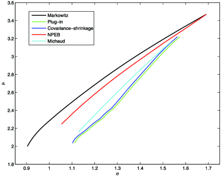
Figure 1: $(\sigma,\mu)$ curves of different portfolios.

Table 1 compares the Bayes rule that maximizes (9), called “Bayes” hereafter, with three other rules: (a) the “oracle” rule that assumes $\bolds{\mu}$ and $\bolds{\Sigma}$ to be known, (b) the plug-in rule that replaces $\bolds{\mu}$ and $\bolds{\Sigma}$ by the sample estimates of $\bolds{\mu}$ and $\bolds{\Sigma}$, and (c) the NPEB (nonparametric empirical Bayes) rule described in Section 4.1 Note that although both (b) and (c) use the sample mean vector and sample covariance (or second moment) matrix, (b) simply plugs the sample estimates into the oracle rule while (c) uses the empirical distribution to replace the common distribution of the returns in the Bayes rule. For the plug-in rule, the quadratic programming procedure may have numerical difficulties if the sample covariance matrix is nearly singular. If it should happen, we use the default option of adding 0.005${\mathbf{I}}$ to the sample covariance matrix. Each result in Table 1 is based on 500 simulations, and the standard errors are given in parentheses. In each scenario, the reward of the NPEB rule is close to that of the Bayes rule and somewhat smaller than that of the oracle rule. The plug-in rule has substantially smaller rewards, especially for larger values of $\lambda$.

4.3 Comparison of the $(\sigma,\mu)$ plots of different portfolios

The set of points in the $(\sigma,\mu)$ plane that correspond to the returns of portfolios of the $m$ assets is called the feasible region. As $\lambda$ varies over $(0,\infty)$, the $(\sigma,\mu)$ values of the oracle rule correspond to Markowitz’s efficient frontier which assumes known $\bolds{\mu}$ and $\bolds{\Sigma}$ and which is the upper left boundary of the feasible region. For portfolios whose weights do not assume knowledge of $\bolds{\mu}$ and $\bolds{\Sigma}$, the $(\sigma,\mu)$ values lie on the right of Markowitz’s efficient frontier. Figure 1 plots the $(\sigma,\mu)$ values of different portfolios formed from $m=4$ assets without short selling and a training sample of size $n=6$ when $(\bolds{\mu},\bolds{\Sigma})$ is given by the frequentist scenario Freq 1 above. Markowitz’s efficient frontier is computed analytically by varying $\mu_{*}$ in (1) over a grid of values. The $(\sigma,\mu)$ curves of the plug-in, covariance-shrinkage [Ledoit and Wolf (2004)] and Michaud’s resampled portfolios are computed by Monte Carlo, using 500 simulated paths, for each value of $\mu_{*}$ in a grid ranging from 2.0 to 3.47. The $(\sigma,\mu)$ curve of the NPEB portfolio is also obtained by Monte Carlo simulations with 500 runs, by using different values of $\lambda>0$ in a grid. This curve is relatively close to Markowitz’s efficient frontier among the $(\sigma,\mu)$ curves of various portfolios that do not assume knowledge of $\bolds{\mu}$ and $\bolds{\Sigma}$, as shown in Figure 1. For the covariance-shrinkage portfolio, we use a constant correlation model for $\widehat{F}$ in (6), which can be implemented by their software available at www.ledoit.net. Note that Markowitz’s efficient frontier has $\mu$ values ranging from 2.0 to 3.47, which is the largest component of $\bolds{\mu}$ in Freq 1. The $(\sigma,\mu)$ curve of NPEB lies below the efficient frontier, and further below are the $(\sigma,\mu)$ curves of Michaud’s, covariance-shrinkage and plug-in portfolios, in decreasing order. These $(\sigma,\mu)$ curves are what Broadie (1993) calls the actual frontiers.

The highest values 3.22, 3.22 and 3.16 of $\mu$ for the plug-in, covariance-shrinkage and Michaud’s portfolios in Figure 1 are attained with a target value $\mu_{*}=3.47$, and the corresponding values of $\sigma$ are 1.54, 1.54 and 3.16, respectively. Note that without short selling, the constraint ${\mathbf{w}}^{T}\widehat{\bolds{\mu}}=\mu_{*}$ used in these portfolios cannot hold if $\max_{1\leq i\leq 4}\widehat{\mu}_{i}<\mu_{*}$. We therefore need a default option, such as replacing $\mu_{*}$ by $\min(\mu_{*},\max_{1\leq i\leq 4}\widehat{\mu}_{i})$, to implement the optimization procedures for these portfolios. In contrast, the NPEB portfolio can always be implemented for any given value of $\lambda$. In particular, for $\lambda=0.001$, the NPEB portfolio has $\mu=3.470$ and $\sigma=1.691$.

5 Connecting theory to practice

While Section 4 has considered practical implementation of the theory in Section 3, we develop the methodology further in this section to connect the basic theory to practice.

5.1 The information ratios and choice of $\lambda$

As pointed out in Section 1, the $\lambda$ in Section 3 is related to how risk-averse one is when one tries to maximize the expected utility of a portfolio. It represents a penalty on the risk that is measured by the variance of the portfolio’s return. In practice, it may be difficult to specify an investor’s risk aversion parameter $\lambda$ that is needed in the theory in Section 3.1. A commonly used performance measure of a portfolio’s performance is the information ratio $(\mu-\mu_{0})/\sigma_{e}$, which is the excess return per unit of risk; the excess is measured by $\mu-\mu_{0}$, where $\mu_{0}=E(r_{0})$, $r_{0}$ is the return of the benchmark investment and $\sigma_{e}^{2}$ is the variance of the excess return. We can regard $\lambda$ as a tuning parameter, and choose it to maximize the information ratio by modifying the NPEB procedure in Section 3.2, where the bootstrap estimate of $E_{\bolds{\mu},\bolds{\Sigma}}[{\mathbf{w}}^{T}(\eta){\mathbf{r}}]-\lambda\operatorname{Var}_{\bolds{\mu},\bolds{\Sigma}}[{\mathbf{w}}^{T}(\eta){\mathbf{r}}]$ is used to find the portfolio weight ${\mathbf{w}}_{\lambda}$ that solves the optimization problem (11). Specifically, we use the bootstrap estimate of the information ratio

$$E_{\bolds{\mu},\bolds{\Sigma}}({\mathbf{w}}_{\lambda}{\mathbf{r}}-r_{0})/\sqrt{\operatorname{Var}_{\bolds{\mu},\bolds{\Sigma}}({\mathbf{w}}_{\lambda}^{T}{\mathbf{r}}-r_{0})}$$ (19)

of ${\mathbf{w}}_{\lambda}$, and maximize the estimated information ratios over $\lambda$ in a grid that will be illustrated in Section 6.

5.2 Dimension reduction when $m$ is not small relative to $n$

Another statistical issue encountered in practice is the large number $m$ of assets relative to the number $n$ of past periods in the training sample, making it difficult to estimate $\bolds{\mu}$ and $\bolds{\Sigma}$ satisfactorily. Using factor models that are related to domain knowledge as in Section 2.1 helps reduce the number of parameters to be estimated in an empirical Bayes approach.

Table 2: Rewards of four portfolios formed from $m=6$ assets

$\bolds\lambda$	$\bolds{(}\bolds{\mu}\bolds{,}\bolds{\Sigma}\bolds{)}$	Bayes	Plug-in	Oracle	NPEB
1	Bayes	0.0325 (2.55e$-$5)	0.0318 (2.62e$-$6)	0.0331 (2.42e$-$5)	0.0325 (2.53e$-$5)
	Freq 1	0.0284 (1.59e$-$5)	0.0277 (1.31e$-$5)	0.0296 (2.62e$-$6)	0.0285 (1.62e$-$5)
	Freq 2	0.0292 (8.30e$-$6)	0.0280 (7.95e$-$6)	0.0296 (2.62e$-$6)	0.0292 (8.29e$-$6)
	Freq 3	0.0283 (1.00e$-$5)	0.0282 (9.11e$-$6)	0.0300 (2.62e$-$6)	0.0283 (1.05e$-$5)
5	Bayes	0.0255 (2.46e$-$5)	0.0183 (1.44e$-$5)	0.0263 (2.05e$-$5)	0.0254 (2.45e$-$5)
	Freq 1	0.0236 (1.99e$-$5)	0.0149 (6.48e$-$6)	0.0250 (2.05e$-$6)	0.0237 (2.17e$-$5)
	Freq 2	0.0241 (9.34e$-$6)	0.0166 (3.61e$-$6)	0.0246 (2.05e$-$6)	0.0243 (8.95e$-$6)
	Freq 3	0.0189 (2.09e$-$5)	0.0138 (1.45e$-$5)	0.0219 (2.05e$-$6)	0.0208 (2.32e$-$5)
10	Bayes	0.0171 (2.63e$-$5)	0.0039 (1.57e$-$5)	0.0180 (2.20e$-$5)	0.0171 (2.72e$-$5)
	Freq 1	0.0174 (2.06e$-$5)	0.0042 (5.19e$-$6)	0.0193 (2.20e$-$6)	0.0177 (2.42e$-$5)
	Freq 2	0.0177 (1.12e$-$5)	0.0052 (6.34e$-$6)	0.0184 (2.20e$-$6)	0.0180 (1.10e$-$5)
	Freq 3	0.0089 (2.79e$-$5)	0.0024 (1.33e$-$5)	0.0120 (2.20e$-$6)	0.0094 (4.65e$-$5)

An obvious way of dimension reduction when there is no short selling is to exclude assets with markedly inferior information ratios from consideration. The only potential advantage of including them in the portfolio is that they may be able to reduce the portfolio variance if they are negatively correlated with the “superior” assets. However, since the correlations are unknown, such advantage is unlikely when they are not estimated well enough. Suppose we include in the simulation study of Section 4.2 two more assets so that all asset returns are jointly normal. The additional hyperparameters of the normal and inverted Wishart prior distribution (4) are $\bolds{\nu}_{5}=-0.014$, $\bolds{\nu}_{6}=-0.064$, $\bolds{\Psi}_{55}=2.02$, $\bolds{\Psi}_{66}=10.32$, $\bolds{\Psi}_{56}=0.90$, $\bolds{\Psi}_{15}=-0.17$, $\bolds{\Psi}_{25}=-0.03$, $\bolds{\Psi}_{35}=-0.91$, $\bolds{\Psi}_{45}=-0.33$, $\bolds{\Psi}_{16}=-3.40$, $\bolds{\Psi}_{26}=-3.99$, $\bolds{\Psi}_{36}=-0.08$ and $\bolds{\Psi}_{46}=-3.58$. As in Section 4.2, we consider four scenarios for the case of $n=8$ without short selling, the first of which assumes this prior distribution and studies the Bayesian reward for $\lambda=1,5$ and 10. Table 2 shows the rewards for the four rules in Section 4.2, and each result is based on 500 simulations. Note that the value of the reward function does not show significant change with the inclusion of two additional stocks, which have negative correlations with the four stocks in Section 4.2 but have low information ratios. This shows that excluding stocks with markedly inferior information ratios when there is no short selling can reduce $m$ substantially in practice. In Section 6 we describe another way of choosing stocks from a universe of available stocks to reduce $m$.

5.3 Extension to time series models of returns

An important assumption in the modification of Markowitz’s theory in Section 3.2 is that ${\mathbf{r}}_{t}$ are i.i.d. with mean $\bolds{\mu}$ and covariance matrix $\bolds{\Sigma}$. Diagnostic checks of the extent to which this assumption is violated should be carried out in practice. The stochastic optimization theory in Section 3.1 does not actually need this assumption and only requires the posterior mean and second moment matrix of the return vector for the next period in (12). Therefore, one can modify the “working i.i.d. model” accordingly when the diagnostic checks reveal such modifications are needed.

A simple method to introduce such modification is to use a stochastic regression model of the form

$$r_{it}=\bolds{\beta}_{i}^{T}{\mathbf{x}}_{i,t-1}+\epsilon_{it},$$ (20)

where the components of ${\mathbf{x}}_{i,t-1}$ include 1, factor variables such as the return of a market portfolio like S&P500 at time $t-1$, and lagged variables $r_{i,t-1},r_{i,t-2},\ldots.$ The basic idea underlying (20) is to introduce covariates (including lagged variables to account for time series effects) so that the errors $\epsilon_{it}$ can be regarded as i.i.d., as in the working i.i.d. model. The regression parameter $\bolds{\beta}_{i}$ can be estimated by the method of moments, which is equivalent to least squares. We can also include heteroskedasticity by assuming that $\epsilon_{it}=s_{i,t-1}(\bolds{\gamma}_{i})z_{it}$, where $z_{it}$ are i.i.d. with mean 0 and variance 1, $\bolds{\gamma}_{i}$ is a parameter vector which can be estimated by maximum likelihood or generalized method of moments, and $s_{i,t-1}$ is a given function that depends on $r_{i,t-1},r_{i,t-2},\ldots.$ A well-known example is the $\operatorname{GARCH}(1,1)$ model

$$\epsilon_{it}=s_{i,t-1}z_{it},\qquad s_{i,t-1}^{2}=\omega_{i}+a_{i}s_{i,t-2}^{2}+b_{i}r_{i,t-1}^{2}$$ (21)

for which $\bolds{\gamma}_{i}=(\omega_{i},a_{i},b_{i})$.

Consider the stochastic regression model (20). As noted in Section 3.2, a key ingredient in the optimal weight vector that solves the optimization problem (9) is $(\bolds{\mu}_{n},{\mathbf{V}}_{n})$, where $\bolds{\mu}_{n}=E({\mathbf{r}}_{n+1}|{\mathcal{R}}_{n})$ and ${\mathbf{V}}_{n}=E({\mathbf{r}}_{n+1}{\mathbf{r}}_{n+1}^{T}|\break{\mathcal{R}}_{n})$. Instead of the classical model of i.i.d. returns, one can combine domain knowledge of the $m$ assets with time series modeling to obtain better predictors of future returns via $\bolds{\mu}_{n}$ and ${\mathbf{V}}_{n}$. The regressors ${\mathbf{x}}_{i,t-1}$ in (20) can be chosen to build a combined substantive–empirical model for prediction; see Section 7.5 of Lai and Xing (2008). Since the model (20) is intended to produce i.i.d. $\bolds{\epsilon}_{t}=(\epsilon_{1t},\ldots,\epsilon_{mt})^{T}$, or i.i.d. ${\mathbf{z}}_{t}=(z_{1t},\dots,z_{mt})^{T}$ after adjusting for conditional heteroskedasticity as in (21), we can still use the NPEB approach to determine the optimal weight vector, bootstrapping from the estimated common distribution of $\bolds{\epsilon}_{t}$ (or ${\mathbf{z}}_{t}$). Note that (20) and (21) models the asset returns separately, instead of jointly in a multivariate regression or multivariate $\operatorname{GARCH}$ model which has too many parameters to estimate. While the vectors $\bolds{\epsilon}_{t}$ (or ${\mathbf{z}}_{t}$) are assumed to be i.i.d., (20) [or (21)] does not assume their components to be uncorrelated since it treats the components separately rather than jointly. The conditional cross-sectional covariance between the returns of assets $i$ and $j$ given ${\mathcal{R}}_{n}$ is given by

$$\operatorname{Cov}(r_{i,n+1},r_{j,n+1}|{\mathcal{R}}_{n})=s_{i,n}(\bolds{\gamma}_{i})s_{j,n}(\bolds{\gamma}_{j})\operatorname{Cov}(z_{i,n+1},z_{j,n+1}|{\mathcal{R}}_{n})$$ (22)

for the model (20) and (21). Note that (21) determines $s_{i,n}^{2}$ recursively from ${\mathcal{R}}_{n}$, and that ${\mathbf{z}}_{n+1}$ is independent of ${\mathcal{R}}_{n}$ and, therefore, its covariance matrix can be consistently estimated from the residuals $\widehat{\mathbf{z}}_{t}$. Under (20) and (21), the NPEB approach uses the following formulas for $\bolds{\mu}_{n}$ and ${\mathbf{V}}_{n}$ in (13):

$$\hskip 25.0pt\bolds{\mu}_{n}=(\widehat{\bolds{\beta}}_{1}^{T}{\mathbf{x}}_{1,n},\dots,\widehat{\bolds{\beta}}_{m}^{T}{\mathbf{x}}_{m,n})^{T},\qquad{\mathbf{V}}_{n}=\bolds{\mu}_{n}\bolds{\mu}_{n}^{T}+(\widehat{s}_{i,n}\widehat{s}_{j,n}\widehat{\sigma}_{ij})_{1\leq i,j\leq n},$$ (23)

in which $\widehat{\bolds{\beta}}_{i}$ is the least squares estimate of $\bolds{\beta}_{i}$, and $\widehat{s}_{l,n}$ and $\widehat{\sigma}_{ij}$ are the usual estimates of $s_{l,n}$ and $\operatorname{Cov}(z_{i,1},z_{j,1})$ based on ${\mathcal{R}}_{n}$. Further discussion of time series modeling for implementing the optimal portfolio in Section 3 will be given in Sections 6.2 and 7.

6 An empirical study

In this section we describe an empirical study of the out-of-sample performance of the proposed approach and other methods for mean–variance portfolio optimization when the means and covariances of the underlying asset returns are unknown. The study uses monthly stock market data from January 1985 to December 2009, which are obtained from the Center for Research in Security Prices (CRSP) database, and evaluates out-of-sample performance of different portfolios of these stocks for each month after the first ten years (120 months) of this period to accumulate training data. The CRSP database can be accessed through the Wharton Research Data Services at the University of Pennsylvania (http://wrds.wharton.upenn.edu). Following Ledoit and Wolf (2004), at the beginning of month $t$, with $t$ varying from January 1995 to December 2009, we select $m=50$ stocks with the largest market values among those that have no missing monthly prices in the previous 120 months, which are used as the training sample. The portfolios for month $t$ to be considered are formed from these $m$ stocks.

Note that this period contains highly volatile times in the stock market, such as around “Black Monday” in 1987, the Internet bubble burst and the September 11 terrorist attacks in 2001, and the “Great Recession” that began in 2007 with the default and other difficulties of subprime mortgage loans. We use sliding windows of $n=120$ months of training data to construct portfolios of the stocks for the subsequent month. In contrast to the Black–Litterman approach described in Section 2.2, the portfolio construction is based solely on these data and uses no other information about the stocks and their associated firms, since the purpose of the empirical study is to illustrate the basic statistical aspects of the proposed method and to compare it with other statistical methods for implementing Markowitz’s mean–variance portfolio optimization theory. Moreover, for a fair comparison, we do not assume any prior distribution as in the Bayes approach, and only use NPEB in this study.

Performance of a portfolio is measured by the excess returns $e_{t}$ over a benchmark portfolio. As $t$ varies over the monthly test periods from January 1995 to December 2009, we can (i) add up the realized excess returns to give the cumulative realized excess return $\sum_{l=1}^{t}e_{l}$ up to time $t$, and (ii) use the average realized excess return and the standard deviation to evaluate the realized information ratio $\sqrt{12}\bar{e}/s_{e}$, where $\bar{e}$ is the sample average of the monthly excess returns and $s_{e}$ is the corresponding sample standard deviation, using $\sqrt{12}$ to annualize the ratio as in Ledoit and Wolf (2004). Noting that the realized information ratio is a summary statistic of the monthly excess returns in the 180 test periods, we find it more informative to supplement this commonly used measure of investment performance with the time series plot of cumulative realized excess returns, from which the realized excess returns $e_{t}$ can be retrieved by differencing.

We use two ways to construct the benchmark portfolio. The first follows that of Ledoit and Wolf (2004), who propose to mimic how an active portfolio manager chooses the benchmark to define excess returns. It is described in Section 6.1. The second simply uses the S&P500 Index as the benchmark portfolio and Section 6.3 considers this case. Section 6.2 compares the time series of the returns of these two benchmark portfolios and explains why we choose to use the S&P500 Index as the benchmark portfolio in conjunction with the time series model (20) and (21) for the excess returns in Section 6.3.

6.1 Active portfolios and associated optimization problems

In this section the benchmark portfolio consists of the $m=50$ stocks chosen at the beginning of each test period and weights them by their market values. Let ${\mathbf{w}}_{B}$ denote the weight of this value-weighted benchmark and ${\mathbf{w}}$ the weight of a given portfolio. The difference $\widetilde{\mathbf{w}}={\mathbf{w}}-{\mathbf{w}}_{B}$ satisfies $\widetilde{\mathbf{w}}^{T}{\mathbf{1}}=0$. An active portfolio manager would choose ${\mathbf{w}}$ that solves the following optimization problem instead of (1):

$${\mathbf{w}}_{\mathrm{active}} = {\mathbf{w}}_{B}+\arg\min_{\widetilde{\mathbf{w}}}\widetilde{\mathbf{w}}^{T}\bolds{\Sigma}\widetilde{\mathbf{w}}\quad\mbox{subject to}\quad\widetilde{\mathbf{w}}^{T}\bolds{\mu}=\widetilde{\mu}_{*},$$

$$\widetilde{\mathbf{w}}^{T}{\mathbf{1}} = 0\mbox{ and }\widetilde{\mathbf{w}}\in{\mathcal{C}},\vspace*{-3pt}$$

in which ${\mathcal{C}}$ represents additional constraints for the manager, $\bolds{\Sigma}$ is the covariance matrix of stock returns and $\widetilde{\mu}_{*}$ is the target excess return over the value-weighted benchmark. The portfolio defined by ${\mathbf{w}}_{\mathrm{active}}$ is called an active portfolio. Since $\bolds{\mu}$ and $\bolds{\Sigma}$ are typically unknown, putting a prior distribution on them in (6.1) leads to the following modification of (9):

$$\max\{E(\widetilde{\mathbf{w}}^{T}{\mathbf{r}}_{n+1})-\lambda\operatorname{Var}(\widetilde{\mathbf{w}}^{T}{\mathbf{r}}_{n+1})\}\quad\mbox{subject to}\quad\widetilde{\mathbf{w}}^{T}{\mathbf{1}}=0.$$ (25)

This optimization problem can be solved by the same method as that introduced in Section 3.

Table 3: Means and standard deviations (in parentheses) of the annualized realized excess returns over the value-based benchmark

$\bolds{\widetilde{\mu}_{*}}$	0.01	0.015	0.02	0.03
$\bolds\lambda$	$\bolds{2^{2}}$	2	$\bolds{2^{-1}}$	$\bolds{2^{-2}}$
(a) All test periods by re-defining portfolios in some periods
Plug-in	0.001 (4.7e$-$3)	0.002 (7.3e$-$3)	0.003 (9.6e$-$3)	0.007 (1.4e$-$2)
Shrink	0.003 (4.3e$-$3)	0.004 (6.6e$-$3)	0.006 (8.8e$-$3)	0.011 (1.3e$-$2)
Boot	0.001 (2.5e$-$3)	0.001 (3.8e$-$3)	0.001 (5.1e$-$3)	0.003 (7.3e$-$3)
NPEB	0.029 (1.2e$-$1)	0.046 (1.3e$-$1)	0.053 (1.5e$-$1)	0.056 (1.6e$-$1)
(b) Test periods in which all portfolios are well defined
Plug-in	0.002 (6.6e$-$3)	0.004 (1.0e$-$2)	0.006 (1.4e$-$2)	0.014 (1.9e$-$2)
Shrink	0.005 (5.9e$-$3)	0.008 (9.0e$-$3)	0.012 (1.2e$-$2)	0.021 (1.8e$-$2)
Boot	0.001 (3.5e$-$3)	0.003 (5.3e$-$3)	0.003 (7.1e$-$3)	0.006 (1.0e$-$2)
NPEB	0.282 (9.3e$-$2)	0.367 (1.1e$-$1)	0.438 (1.1e$-$1)	0.460 (1.1e$-$2)

Following Ledoit and Wolf (2004), we choose the constraint set ${\mathcal{C}}$ such that the portfolio is long only and the total position in any stock cannot exceed an upper bound $c$, that is, ${\mathcal{C}}=\{\widetilde{\mathbf{w}}\dvtx-{\mathbf{w}}_{B}\leq\widetilde{\mathbf{w}}\leq c{\mathbf{1}}-{\mathbf{w}}_{B}\}$, with $c=0.1$. We use quadratic programming to solve the optimization problem (6.1) in which $\bolds{\mu}$ and $\bolds{\Sigma}$ are replaced, for the plug-in active portfolio, by their sample estimates based on the training sample in the past 120 months. The covariance-shrinkage active portfolio uses a shrinkage estimator of $\bolds{\Sigma}$ instead, shrinking toward a patterned matrix that assumes all pairwise correlations to be equal [Ledoit and Wolf (2003)]. Similarly, we can extend Section 2.3 to obtain a resampled active portfolio, and also extend the NPEB approach in Section 4 to construct the corresponding NPEB active portfolio. Table 3 summarizes the realized information ratio $\sqrt{12}\bar{e}/s_{e}$ for different values of annualized target excess returns $\widetilde{\mu}_{*}$ and “matching” values of $\lambda$ whose choice is described below.

We first note that specified target returns $\widetilde{\mu}_{*}$ may be vacuous for the plug-in, covariance-shrinkage (abbreviated “shrink” in Table 3) and resampled (abbreviated “boot” for bootstrapping) active portfolios in a given test period. For $\widetilde{\mu}_{*}=0.01,0.015,0.02,0.03$, there are 92, 91, 91 and 80 test periods, respectively, for which (6.1) has solutions when $\bolds{\Sigma}$ is replaced by either the sample covariance matrix or the Ledoit–Wolf shrinkage estimator of the training data from the previous 120 months. Higher levels of target returns result in even fewer of the 180 test periods for which (6.1) has solutions. On the other hand, values of $\widetilde{\mu}_{*}$ that are lower than 1% may be of little practical interest to active portfolio managers. When (6.1) does not have a solution to provide a portfolio of a specified type for a test period, we use the value-weighted benchmark as the portfolio for the test period. Table 3(a) gives the actual (annualized) mean realized excess returns $12\bar{e}$ to show the extent to which they match the target value $\widetilde{\mu}_{*}$, and also the corresponding annualized standard deviations $\sqrt{12}s_{e}$, over the 180 test periods for the plug-in, covariance-shrinkage and resampled active portfolios constructed with the above modification. These numbers are very small, showing that the three portfolios differ little from the benchmark portfolio, so the realized information ratios that range from 0.24 to 0.83 for these active portfolios can be quite misleading if the actual mean excess returns are not taken into consideration.

We have also tried another default option that uses 10 stocks with the largest mean returns (among the 50 selected stocks) over the training period and puts equal weights to these 10 stocks to form a portfolio for the ensuing test period for which (6.1) does not have a solution. The mean realized excess returns $12\bar{e}$ when this default option is used are all negative (between $-$17.4% and $-$16.3%), while $\widetilde{\mu}_{*}$ ranges from 1% from 3%. Table 3(a) also gives the means and standard deviations of the annualized realized excess returns of the NPEB active portfolio for four values of $\lambda$ that are chosen so that the mean realized excess returns roughly match the values of $\widetilde{\mu}_{*}$ over a grid of the form $\lambda=2^{j}$ $(-2\leq j\leq 2)$ that we have tried. Note that NPEB has considerably larger mean excess returns than the other three portfolios.

Table 3(b) restricts only to the 80–92 test periods in which the plug-in, covariance-shrinkage and resampled active portfolios are all well defined by (6.1) for $\widetilde{\mu}_{*}=0.01,0.015,0.02$ and 0.03. The mean excess returns of the plug-in, covariance-shrinkage and resampled portfolios are still very small, while those of NPEB are much larger. The realized information ratios of NPEB range from 3.015 to 3.954, while those of the other three portfolios range from 0.335 to 1.214 when we restrict to these test periods.

6.2 Value-weighted portfolio versus S&P500 Index and time series effects

The results for the plug-in and covariance-shrinkage portfolios in Table 3 are markedly different from those of Ledoit and Wolf (2004) covering a different period (February 1983–December 2002). This suggests that the stock returns cannot be approximated by the assumed i.i.d. model underlying these methods. In Section 5.3 we have extended the NPEB approach to a very flexible time series model (20) and (21) of the stock returns $r_{it}$. The stochastic regression model (20) can incorporate important time-varying predictors in ${\mathbf{x}}_{it}$ for the $i$th stock’s performance at time $t$, while the $\operatorname{GARCH}$ model (21) for the random disturbances $\epsilon_{it}$ in (20) can incorporate dynamic features of the stock’s idosyncratic variability. It seems that a regressor such as the return $u_{t}$ of S&P500 Index should be included in ${\mathbf{x}}_{it}$ to take advantage of the co-movements of $r_{it}$ and $u_{t}$. However, since $u_{t}$ is not observed at time $t$, one may need to have good predictors of $u_{t}$ which should consist not only of the past S&P500 returns but also macroeconomic variables. Of course, stock-specific information such as the firm’s earnings performance and forecast and its sector’s economic outlook should also be considered. This means that fundamental analysis, as carried out by professional stock analysts and economists in investment banks, should be incorporated into the model (20). Since this is clearly beyond the scope of the present empirical study whose purpose is to illustrate our new statistical approach to the Markowitz optimization enigma, we shall focus on simple models to demonstrate the benefit of building good models for ${\mathbf{r}}_{t+1}$ in our stochastic optimization approach.

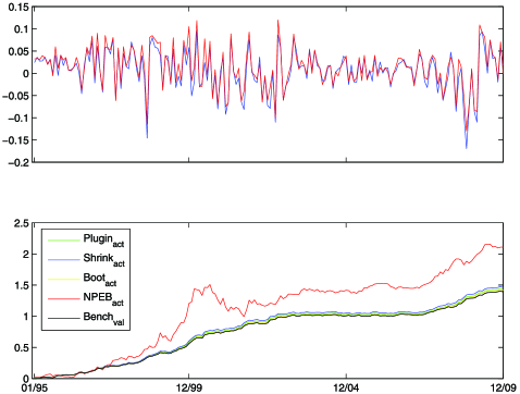
Figure 2: Time series plots of the monthly returns (Top) of the S&P500 Index and the value-weighted benchmark, and cumulative excess returns (Bottom) of the value-weighted benchmark (abbreviated by Bench_val) and for active portfolios (abbreviated by the subscript “act”) over the S&P500 Index.

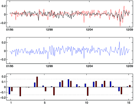
Figure 3: Comparison of returns and excess returns. Top panel: returns of S&P500 Index (black) and SHW (red). Middle panel: excess returns (blue) of SHW. Bottom panel: Autocorrelations of returns (red) and excess returns (blue) of SHW; the dotted lines represent rejection boundaries of 5%-level tests of zero autocorrelation at indicated lag.

In this connection, we first compare the S&P500 Index with the value-weighted portfolio, which is the benchmark portfolio in Section 6.1. The top panel of Figure 2 gives the time series plots of the monthly returns (which are not annualized) of both portfolios during the test period. The S&P500 Index has mean 0.006 and standard deviation 0.046 in this period, while the mean of the value-weighted portfolio is 0.0137 and its standard deviation is 0.045. The bottom panel of Figure 2 plots the time series of cumulative realized excess returns $\sum_{l=1}^{t}e_{l}$ over the S&P500 Index, for the value-weighted portfolio and also for the four active portfolios in Table 3(a) under the column $\mu_{*}=0.015$ and $\lambda=2$, during the test period (January 1995–December 2009). Unlike NPEB_act, the cumulative realized excess returns of the other three active portfolios differ little from the value-weighted portfolio, as shown by the figure.

In view of the structural changes in the economy and the financial markets during this period, it appears difficult to find simple time series models that can reflect the inherent nonstationarity. If we use the S&P500 Index $u_{t}$ as an alternative benchmark to the value-weighted portfolio used in Section 6.1, the excess returns $e_{it}=r_{it}-u_{t}$ may be able to exploit the co-movements of $r_{it}$ and $u_{t}$ to remove their common nonstationarity due to changes in macroeconomic variables. As an illustration, the top panel of Figure 3 gives the time series plots of returns of Sherwin–Williams Co. (SHW) and of the S&P500 Index during this period, and the middle panel gives the time series plot of the excess returns. The Ljung–Box test, which involves autocorrelations of lags up to 20 months, has $p$-value 0.001 for the monthly returns of SHW and 0.267 for the excess returns, and therefore rejects the i.i.d. assumption for the actual but not the excess returns; see Section 5.1 of Lai and Xing (2008). This is also shown graphically by the autocorrelation functions in the bottom panel of Figure 3.

6.3 Using the S&P500 Index as benchmark portfolio and time series models of excess returns

The preceding section shows that using the S&P500 Index as the benchmark portfolio has certain advantages over the value-weighted portfolio. In this section we consider the excess returns $e_{it}$ over the S&P500 Index $u_{t}$, which we use as the benchmark portfolio, and fit relatively simple time series models to the training sample to predict the mean and volatility of $e_{it}$ for the test period. Instead of forming active portfolios as in Section 6.1, we follow traditional portfolio theory as described in Sections 1–3. Note that this theory assumes the constraint $\sum_{i=1}^{m}w_{i}=1$ and, therefore,

$$\sum_{i=1}^{m}w_{i}r_{it}-u_{t}=\sum_{i=1}^{m}w_{i}(r_{it}-u_{t})=\sum_{i=1}^{m}w_{i}e_{it},$$ (26)

whereas active portfolio optimization considers weights $\widetilde{w}_{i}=w_{i}-w_{i,B}$ that satisfy the constraint $\sum_{i=1}^{m}\widetilde{w}_{i}=0$. In view of (26), when the objective is to maximize the mean return of the portfolio subject to a constraint on the volatility of the excess return over the benchmark (which is related to achieving an optimal information ratio), we can replace the returns $r_{it}$ by the excess returns $e_{it}$ in the portfolio optimization problem (1) or (9). As explained in the second paragraph of Section 6.2, $e_{it}$ can be modeled by simpler stationary time series models than $r_{it}$.

The simplest time series model to try is the $\operatorname{AR}(1)$ model $e_{it}=\alpha_{i}+\gamma_{i}e_{i,t-1}+\epsilon_{it}$. Assuming this time series model for the excess returns, we can apply the NPEB procedure in Section 5.3 to the training sample and thereby obtain the NPEB${}_{\operatorname{AR}}$ portfolio for the test sample. The $\operatorname{AR}(1)$ model uses ${\mathbf{x}}_{i,t-1}=(1,e_{i,t-1})^{T}$ as the predictor in a linear regression model for $e_{i,t}$. To improve prediction performance, one can include additional predictor variables, for example, the return $u_{t-1}$ of the S&P500 Index in the preceding period. Assuming the stochastic regression model $e_{i,t}=(1,e_{i,t-1},u_{t-1})\bolds{\beta}_{i}+\epsilon_{i,t}$, and the $\operatorname{GARCH}(1,1)$ model (21) for $\epsilon_{i,t}$, we can apply the NPEB procedure to the training sample and thereby form the NPEB_SRG portfolio for the test sample.

Instead of taking long-only positions (i.e., $w_{i}\geq 0$ for all $i$), we also allow short selling, with the constraint $w_{i}\geq-0.05$ for all $i$, to construct the following portfolios in this section. For the plug-in, covariance-shrinkage and resampled portfolios, which we abbreviate as in Figure 2 but without the subscript “act” (for active), we use the annualized target return $\mu_{*}=0.015,0.02,0.03$, for which the problem (1) can be solved for all 180 test periods under the weight constraint; note that we use the mean return instead of the mean excess return as the target $\mu_{*}$. For the NPEB${}_{\operatorname{AR}}$ and NPEB_SRG portfolios, we use the training sample as in Section 5.1 to choose $\lambda$ by maximizing the information ratio over the grid $\lambda\in\{2^{i}\dvtx i=-3,-2,\dots,6\}$. Figure 4 plots the time series of cumulative realized excess returns over the S&P500 Index during the test period of 180 months, for Plug-in, Shrink and Boot with $\mu_{*}=0.015$ and for NPEB${}_{\operatorname{AR}}$ and NPEB_SRG. Table 4 gives the annualized realized information ratios, with the S&P500 Index as the benchmark portfolio. The table also considers cases $\mu_{*}=0.02,0.03$, and further abbreviates Plug-in, Shrink and Boot by P, S, B, respectively.

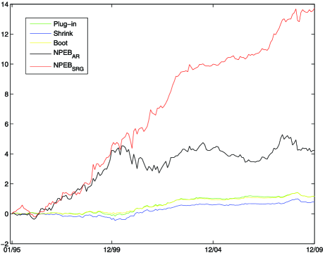
Figure 4: Realized cumulative excess returns over the S&P500 Index.

Table 4: Realized information ratios and average realized excess returns (in square brackets) with respect to the S&P500 Index

$\bolds{\mu_{*}=0.015}$			$\bolds{\mu_{*}=0.02}$			$\bolds{\mu_{*}=0.03}$			NPEB
P	S	B	P	S	B	P	S	B	$\bolds{\operatorname{AR}}$	SRG
0.527	0.352	0.618	0.532	0.353	0.629	0.538	0.354	0.625	0.370	1.169
[0.078]	[0.052]	[0.077]	[0.078]	[0.051]	[0.078]	[0.076]	[0.050]	[0.077]	[0.283]	[0.915]

6.4 Discussion

Our approach may perform much better if the investor can combine domain knowledge with the statistical modeling that we illustrate here. We have not done this in the present comparative study because using a purely empirical analysis of the past returns of these stocks to build the prediction model (20) would be a disservice to the power and versatility of the proposed approach, which is developed in Section 3 in a general Bayesian framework, allowing the skillful investor to make use of prior beliefs on the future return vector ${\mathbf{r}}_{n+1}$ and statistical models for predicting ${\mathbf{r}}_{n+1}$ from past market data. The prior beliefs can involve both the investor’s and the market’s “views,” as in the Black–Litterman approach described in Section 2.2, for which the market’s view is implied by the equilibrium portfolio. Note that Black and Litterman model the potential errors of these views by normal priors whose covariance matrices reflect the uncertainties. Our Bayesian approach goes one step further to account for these uncertainties by using the actual means and variances of the portfolio’s return in the optimization problem (9), instead of the estimated means and variances in the plug-in approach.

A portfolio on Markowitz’s efficient frontier can be interpreted as a minimum-variance portfolio achieving a target mean return, or a maximum-mean portfolio at a given volatility (i.e., standard derivation of returns). Portfolio managers prefer the former interpretation, as target returns are appealing to investors. In active portfolio management [Grinold and Kahn (2000)], this has led to the target excess return $\widetilde{\mu}_{*}$ and the optimization problem (6.1). The empirical study in Section 6.1 shows that when the means and covariances of the stock returns are unknown and are estimated from historical data, putting these estimates in (6.1) may not provide a solution; moreover, the actual mean of the solution (when it exists) can differ substantially from $\widetilde{\mu}_{*}$.

7 Concluding remarks

The “Markowitz enigma” has been attributed to (a) sampling variability of the plug-in weights (hence use of resampling to correct for bias due to nonlinearity of the weights as a function of the mean vector and covariance matrix of the stocks) or (b) inherent difficulties of estimation of high-dimensional covariance matrices in the plug-in approach. Like the plug-in approach, subsequent refinements that attempt to address (a) or (b) still follow closely Markowitz’s solution for efficient portfolios, constraining the unknown mean to equal to some target returns. This tends to result in relatively low information ratios when no or limited short selling is allowed, as noted in Sections 4.3 and 6. Another difficulty with the plug-in and shrinkage approaches is that their measure of “risk” does not account for the uncertainties in the parameter estimates. Incorporating these uncertainties via a Bayesian approach results in a much harder stochastic optimization problem than Markowitz’s deterministic optimization problem, which we have been able to solve by introducing an additional parameter $\eta$.

Our solution of this stochastic optimization problem opens up new possibilities in extending Markowitz’s mean–variance portfolio optimization theory to the case where the means and covariances of the asset returns for the next investment period are unknown. As pointed out in Section 5.3, our solution only requires the posterior mean and second moment matrix of the return vector for the next period, and one can combine the Black–Litterman-type expert views with statistical modeling to develop Bayesian or empirical Bayes models with good predictive properties, for example, by using (20) with suitably chosen ${\mathbf{x}}_{i,t-1}$.

References

- (1) Best, M. J. and Grauer, R. R. (1991). On the sensitivity of mean–variance-efficient portfolios to changes in asset means: Some analytical and computational results. Rev. Fin. Stud. 4 315–342.
- (2) Bickel, P. J. and Levina, E. (2008). Regularized estimation of large covariance matrices. Ann. Statist. 36 199–227. \MR2387969
- (3) Black, F. and Litterman, R. (1990). Asset Allocation: Combining Investor Views with Market Equilibrium. Goldman, Sachs and Co., New York.
- (4) Britten-Jones, M. (1999). The sampling error in estimates of mean–variance efficient portfolio weights. J. Finance 54 655–671.
- (5) Broadie, M. (1993). Computing efficient frontiers using estimated parameters. Ann. Oper. Res. 45 (Special Issue on Financial Engineering) 21–58.
- (6) Canner, N., Mankiw, G. and Weil, D. N. (1997). An asset allocation puzzle. Amer. Econ. Rev. 87 181–191.
- (7) Chopra, V. K., Hensel, C. R. and Turner, A. L. (1993). Massaging mean–variance inputs: Returns from alternative global investment strategies in the 1980s. Management Sci. 39 845–855.
- (8) Fabozzi, F. J., Kolm, P. N., Pachamanova, P. A. and Focardi, S. M. (2007). Robust Portfolio Optimization and Management. Wiley, New York.
- (9) Fan, J., Fan, Y. and Lv, J. (2008). High dimensional covariance matrix estimation using a factor model. J. Econometrics 147 186–197. \MR2472991
- (10) Frankfurter, G. M., Phillips, H. E. and Seagle, J. P. (1976). Performance of the Sharpe portfolio selection model: A comparison. J. Financ. Quant. Anal. 6 191–204.
- (11) Grinold, R. C. and Kahn, R. N. (2000). Active Portfolio Management, 2nd ed. McGraw-Hill, New York.
- (12) Huang, J. Z., Liu, N., Pourahmadi, M. and Liu, L. (2006). Covariance matrix selection and estimation via penalized normal likelihood. Biometrika 93 85–98. \MR2277742
- (13) Jobson, J. D. and Korkie, B. (1980). Estimation for Markowitz efficient portfolios. J. Amer. Statist. Assoc. 75 544–554. \MR0590686
- (14) Jorion, P. (1986). Bayes–Stein estimation for portfolio analysis. J. Financ. Quant. Anal. 21 279–292.
- (15) Lai, T. L. and Xing, H. (2008). Statistical Models and Methods for Financial Markets. Springer, New York. \MR2434025
- (16) Ledoit, P. and Wolf, M. (2003). Improved estimation of the covariance matrix of stock returns with an application to portfolio selection. J. Empirical Finance 10 603–621.
- (17) Ledoit, P. and Wolf, M. (2004). Honey, I shrunk the sample covariance matrix. J. Portfolio Management 30 110–119.
- (18) Markowitz, H. M. (1952). Portfolio selection. J. Finance 7 77–91.
- (19) Markowitz, H. M. (1959). Portfolio Selection. Wiley, New York. \MR0103768
- (20) Meucci, A. (2005). Risk and Asset Allocation. Springer, New York. \MR2155219
- (21) Meucci, A. (2010). The Black–Litterman approach: Original model and extensions. In The Encyclopedia of Quantitative Finance (R. Cont, ed.) 1 196–199. Wiley, New York.
- (22) Michaud, R. O. (1989). Efficient Asset Management. Harvard Business School Press, Boston, MA.
- (23) Press, W. H., Teukolsky, S. A., Wetterling, W. T. and Flannery, B. P. (1992). Numerical Recipes in C, 2nd ed. Cambridge Univ. Press, Cambridge. \MR1201159
- (24) Ross, S. A. (1976). The arbitrage theory of capital asset pricing. J. Econ. Theory 13 341–360. \MR0429063
- (25) Sharpe, W. F. (1964). Capital asset prices: A theory of market equilibrium under conditions of risk. J. Finance 19 425–442.
- (26) Simann, Y. (1997). Estimation risk in portfolio selection: The mean variance model versus the mean absolute deviation model. Management Sci. 43 1437–1446.