Computation of copulas by Fourier methods

Abstract.

We provide an integral representation for the (implied) copulas of dependent random variables in terms of their moment generating functions. The proof uses ideas from Fourier methods for option pricing. This representation can be used for a large class of models from mathematical finance, including Lévy and affine processes. As an application, we compute the implied copula of the NIG Lévy process which exhibits notable time-dependence.

1. Introduction

Copulas provide a complete characterization of the dependence structure between random variables and link in a very elegant way the joint distribution with the marginal distributions via Sklar’s Theorem. However, they are a rather static concept and do not blend well with stochastic processes which can be used to describe the random evolution of dependent quantities, e.g. the evolution of several stock prices. Therefore other methods to create dependence in stochastic models have been developed. Multivariate stochastic processes spring immediately to mind, for example Lévy or affine processes (cf. e.g. Sato 1999, Duffie, Filipović, and Schachermayer 2003, Cuchiero, Filipović, Mayerhofer, and Teichmann 2011 or Muhle-Karbe, Pfaffel, and Stelzer 2012), while in mathematical finance models using time-changes or linear mixture models have been developed; see e.g. Luciano and Schoutens (2006), Luciano and Semeraro (2010), Kawai (2009), Eberlein and Madan (2010) or Khanna and Madan (2009), to mention just a small part of the existing literature. In these approaches however the copula is typically not known explicitly. Another very interesting approach is due to Kallsen and Tankov (2006), who introduced Lévy copulas to characterize the dependence structure of Lévy processes.

In this note, we provide a new representation for the (implied) copula of a multidimensional random variable in terms of its moment generating function. The derivation of the main result borrows ideas from Fourier methods for option pricing, and the motivation stems from the knowledge of the moment generating function in most of the aforementioned models. This paper is organized as follows: in Section 2 we provide the representation of the copula in terms of the moment generating function; the results are proved for random variables for simplicity, while stochastic processes are considered as a corollary. In Section 3 we provide two examples to showcase how this method can be applied, for example, in performing sensitivity analysis of the copula with respect to the parameters of the model. Finally, Section 4 concludes with some remarks.

2. Copulas via Fourier transform methods

Let $\mathbb{R}^{n}$ denote the $n$-dimensional Euclidean space, $\langle\cdot,\cdot\rangle$ the Euclidean scalar product and $\mathbb{R}^{n}_{-}$ the negative orthant, i.e. $\mathbb{R}^{n}_{-}=\{x\in\mathbb{R}^{n}:x_{i}<0\,\,\forall i\}$. We consider a random variable $X=(X_{1},\dots,X_{n})^{\top}\in\mathbb{R}^{n}$ defined on a probability space $(\Omega,\mathcal{F},\mathrm{I\kern-1.99997ptP})$. We denote by $F$ the cumulative distribution function (cdf) of $X$ and by $f$ its probability density function (pdf). Let $C$ denote the copula of $X$ and $c$ its copula density function. Analogously, let $F_{i}$ and $f_{i}$ denote the cdf and pdf respectively of the marginal $X_{i}$, for all $i\in\{1,\dots,n\}$. In addition, we denote by $F_{i}^{-1}$ the generalized inverse of $F_{i}$, i.e. $F_{i}^{-1}(u)=\inf\{v\in\mathbb{R}:F_{i}(v)\geq u\}$.

We denote by $M_{X}$ the (extended) moment generating function of $X$:

$$M_{X}(u)=\mathrm{I\kern-1.99997ptE}\big{[}\mathrm{e}^{\langle u,X\rangle}\big{]},$$ (2.1)

for all $u\in\mathbb{C}^{n}$ such that $M_{X}(u)$ exists. Let us also define the set

$$\mathcal{I}=\big{\{}R\in\mathbb{R}^{n}:M_{X}(R)<\infty\text{ and }M_{X}(R+\mathrm{i}\cdot)\in L^{1}(\mathbb{R}^{n})\big{\}}.$$

In the sequel, we will assume that the following condition is in force.

Assumption ($\mathbb{D}$).

$\mathcal{R}:=\mathcal{I}\cap\mathbb{R}^{n}_{-}\neq\emptyset$.

Remark 2.1.

The integrability of the moment generating function required by Assumption $(\mathbb{D})$ has the following implications:

1. the distribution function $F$ is absolutely continuous with respect to the Lebesgue measure;

2. the density function $f$ is bounded and continuous;

3. the marginal distribution functions $F_{i}$ are also absolutely continuous.

See Sato (1999, Proposition 2.5) for (a) and (b) and Jacod and Protter (2003, Theorem 12.2) for (c).

Theorem 2.2.

Let $X$ be a random variable that satisfies Assumption $(\mathbb{D})$. The copula of $X$ is provided by

$$C(u) =\frac{1}{(-2\pi)^{n}}\int_{\mathbb{R}^{n}}M_{X}(R+\mathrm{i}v)\frac{\mathrm{e}^{-\langle R+\mathrm{i}v,x\rangle}}{\prod_{i=1}^{n}(R_{i}+\mathrm{i}v_{i})}\mathrm{d}v\Big{|}_{x_{i}=F_{i}^{-1}(u_{i})},$$ (2.2)

where $u\in[0,1]^{n}$ and $R\in\mathcal{R}$.

Proof.

Assumption $(\mathbb{D})$ implies that $F_{1},\dots,F_{n}$ are continuous and we know from Sklar’s Theorem that the copula of $X$ is unique and provided by

$$C(u_{1},\dots,u_{n})=F\big{(}F_{1}^{-1}(u_{1}),\dots,F_{n}^{-1}(u_{n})\big{)};$$ (2.3)

see e.g. McNeil, Frey, and Embrechts (2005, Theorem 5.3) for a proof in this setting and Rüschendorf (2009) for an elegant proof in the general case.

We will evaluate the joint cdf $F$ using the methodology of Fourier methods for option pricing. That is, we will think of the cdf as the ‘price’ of a digital option on several fictitious assets. Let us define the function

$$g(y)=1_{\{y_{1}\leq x_{1},\dots,y_{n}\leq x_{n}\}}(y),\quad x,y\in\mathbb{R}^{n},$$ (2.4)

and denote by $\widehat{g}$ its Fourier transform. Then we have that

$$F(x) =\mathrm{I\kern-1.99997ptP}(X_{1}\leq x_{1},\dots,X_{n}\leq x_{n})$$

$$=\mathrm{I\kern-1.99997ptE}\big{[}1_{\{X_{1}\leq x_{1},\dots,X_{n}\leq x_{n}\}}\big{]}=\mathrm{I\kern-1.99997ptE}[g(X)]$$

$$=\frac{1}{(2\pi)^{n}}\int_{\mathbb{R}^{n}}M_{X}(R+\mathrm{i}v)\widehat{g}(\mathrm{i}R-v)\mathrm{d}v,$$ (2.5)

where we have applied Theorem 3.2 in Eberlein, Glau, and Papapantoleon (2010). The prerequisites of this theorem are satisfied due to Assumption $(\mathbb{D})$ and because $g_{R}\in L^{1}(\mathbb{R}^{n})$, where $g_{R}(x):=\mathrm{e}^{-\langle R,x\rangle}g(x)$ for $R\in\mathbb{R}^{n}_{-}$.

Finally, the statement follows from (2.3) and (2) once we have computed the Fourier transform of $g$. We have for $R_{i}<0$, $i\in\{1,\dots,n\}$,

$$\widehat{g}(\mathrm{i}R-v) =\int_{\mathbb{R}^{n}}\mathrm{e}^{\mathrm{i}\langle\mathrm{i}R-v,y\rangle}g(y)\mathrm{d}y$$

$$=\int_{\mathbb{R}^{n}}\mathrm{e}^{\mathrm{i}\langle\mathrm{i}R-v,y\rangle}1_{\{y_{1}\leq x_{1},\dots,y_{n}\leq x_{n}\}}\mathrm{d}y$$

$$=\prod_{i=1}^{n}\int_{-\infty}^{x_{i}}\mathrm{e}^{(-R_{i}-\mathrm{i}v_{i})y_{i}}\mathrm{d}y_{i}$$

$$=(-1)^{n}\prod_{i=1}^{n}\frac{\mathrm{e}^{-(R_{i}+\mathrm{i}v_{i})x_{i}}}{R_{i}+\mathrm{i}v_{i}},$$ (2.6)

which concludes the proof. ∎

Remark 2.3.

If the moment generating function of the marginals is known, the inverse function can be easily computed numerically. We have that

$$F_{i}^{-1}(u) =\inf\{v\in\mathbb{R}:F_{i}(v)\geq u\}$$

$$=\inf\{v\in\mathbb{R}:\mathrm{I\kern-1.99997ptE}\big{[}1_{\{X_{i}\leq v\}}\big{]}\geq u\},$$

where the expectation can be computed using (2) again, while a root finding algorithm provides the infimum (using the continuity of $F_{i}$).

We can also compute the copula density function using Fourier methods, which resembles the computation of Greeks in option pricing.

Lemma 2.4.

Let $X$ be a random variable that satisfies Assumption $(\mathbb{D})$ and assume further that the marginal distribution functions $F_{1},\dots,F_{n}$ are strictly increasing and continuously differentiable. Then, the copula density function $c$ of $X$ is provided by

$$c(u) =\frac{1}{(2\pi)^{n}\prod_{i=1}^{n}f_{i}(x_{i})}\int_{\mathbb{R}^{n}}M_{X}(R+\mathrm{i}v)\,\mathrm{e}^{-\langle R+\mathrm{i}v,x\rangle}\mathrm{d}v\Big{|}_{x_{i}=F_{i}^{-1}(u_{i})},$$ (2.7)

where $u\in(0,1)^{n}$ and $R\in\mathcal{R}$.

Proof.

The distribution functions $F$ and $F_{1},\dots,F_{n}$ are absolutely continuous hence the copula density exists, cf. McNeil et al. (2005, p. 197). Let $u\in(0,1)^{n}$, then we have that $x_{i}=F_{i}^{-1}(u_{i})$ is finite for every $i\in\{1,\dots,n\}$, hence $\mathrm{e}^{-\langle R,x\rangle}$ is bounded. Using Assumption $(\mathbb{D})$ we get that the function $M_{X}(R+\mathrm{i}v)\mathrm{e}^{-\langle R+\mathrm{i}v,x\rangle}$ is integrable and we can interchange differentiation and integration. Then we have that

$$c(u) =\frac{\partial^{n}}{\partial u_{1}\dots\partial u_{n}}C(u_{1},\dots,u_{n})$$

$$=\frac{\partial^{n}}{\partial u_{1}\dots\partial u_{n}}\frac{1}{(-2\pi)^{n}}\int_{\mathbb{R}^{n}}M_{X}(R+\mathrm{i}v)\frac{\mathrm{e}^{-\langle R+\mathrm{i}v,x\rangle}}{\prod_{i=1}^{n}(R_{i}+\mathrm{i}v_{i})}\Big{|}_{x_{i}=F_{i}^{-1}(u_{i})}\mathrm{d}v$$

$$=\frac{1}{(-2\pi)^{n}}\int_{\mathbb{R}^{n}}\frac{M_{X}(R+\mathrm{i}v)}{\prod_{i=1}^{n}(R_{i}+\mathrm{i}v_{i})}\frac{\partial^{n}}{\partial u_{1}\dots\partial u_{n}}\mathrm{e}^{-\langle R+\mathrm{i}v,x\rangle}\Big{|}_{x_{i}=F_{i}^{-1}(u_{i})}\mathrm{d}v.$$ (2.8)

Now, since the marginal distribution functions are continuously differentiable, using the chain rule and the inverse function theorem we get that

$$\frac{\partial^{n}}{\partial u_{1}\dots\partial u_{n}}\left(\mathrm{e}^{-\langle R+\mathrm{i}v,x\rangle}\Big{|}_{x_{i}=F_{i}^{-1}(u_{i})}\right)\\ =(-1)^{n}\prod_{i=1}^{n}(R_{i}+\mathrm{i}v_{i})\mathrm{e}^{-\langle R+\mathrm{i}v,x\rangle}\frac{1}{\prod_{i=1}^{n}f_{i}(x_{i})}\Big{|}_{x_{i}=F_{i}^{-1}(u_{i})},$$ (2.9)

which combined with (2) yields the required result. ∎

A natural application of these representations is for the calculation of the copula of a random variable $X_{t}$ from a multidimensional stochastic process $X=(X_{t})_{t\geq 0}$. There are many examples of stochastic processes where the corresponding characteristic functions are known explicitly. Prominent examples are Lévy processes, self-similar additive (‘Sato’) processes and affine processes.

Corollary 2.5.

Let $X=(X_{t})_{t\geq 0}$ be an $\mathbb{R}^{n}$-valued stochastic process on a basis $(\Omega,\mathcal{F},(\mathcal{F}_{t})_{t\geq 0},\mathrm{I\kern-1.99997ptP})$. Assume that the random variable $X_{t}$, $t\geq 0$, satisfies Assumption $(\mathbb{D})$. Then, the copula of $X_{t}$ is provided by

$$C_{t}(u) =\frac{1}{(-2\pi)^{n}}\int_{\mathbb{R}^{n}}M_{X_{t}}(R+\mathrm{i}v)\frac{\mathrm{e}^{-\langle R+\mathrm{i}v,x\rangle}}{\prod_{i=1}^{n}(R_{i}+\mathrm{i}v_{i})}\mathrm{d}v\Big{|}_{x_{i}=F_{X_{t}^{i}}^{-1}(u_{i})},$$ (2.10)

where $u\in[0,1]^{n}$ and $R\in\mathcal{R}$. An analogous statement holds for the copula density function $c_{t}$ of $X_{t}$.

3. Examples

We will demonstrate the applicability and flexibility of Fourier methods for the computation of copulas using two examples. First we consider a 2D normal random variable and next a 2D normal inverse Gaussian (NIG) Lévy process. Although the copula of the normal random variable is the well-known Gaussian copula, little was known about the copula of the NIG distribution until recently; see Theorem 5.13 in Schmidt (2003) for a special case. v. Hammerstein (2011, Chapter 2) has now provided a general characterization of the (implied) copula of the multidimensional NIG distribution using properties of normal mean-variance mixtures.

Example 3.1.

The first example is simply a ‘sanity check’ for the proposed method. We consider the 2-dimensional Gaussian distribution and compute the corresponding copula for correlation values equal to $\rho=\{-1,0,1\}$; see Figure 3.1 for the resulting contour plots. Of course, the copula of this example is the Gaussian copula, which for correlation coefficients equal to $\{-1,0,1\}$ corresponds to the countermonotonicity copula, the independence copula and the comonotonicity copula respectively. This is also evident from Figure 3.1.

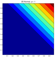
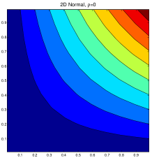
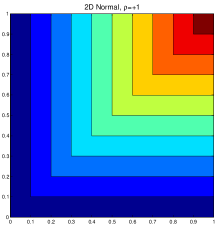
Figure 3.1. Contour plots of copulas for Example 3.1.

Example 3.2.

Let $X=(X_{t})_{t\geq 0}$ be a 2-dimensional NIG Lévy process, i.e.

$$X_{t}=(X_{t}^{1},X_{t}^{2})\sim\text{NIG}_{2}(\alpha,\beta,\delta t,\mu t,\Delta),\quad t\geq 0.$$ (3.1)

The parameters satisfy: $\alpha,\delta>0$, $\beta,\mu\in\mathbb{R}^{2}$, and $\Delta\in\mathbb{R}^{2\times 2}$ is a symmetric, positive definite matrix (w.l.o.g. we can assume $\text{det}(\Delta)=1$). Moreover, $\alpha^{2}>\langle\beta,\Delta\beta\rangle$. The moment generating function of $X_{1}$, for $u\in\mathbb{R}^{2}$ with $\alpha^{2}-\langle\beta+u,\Delta(\beta+u)\rangle\geq 0$, is

$$M_{X_{1}}(u) =\exp\left(\langle u,\mu\rangle+\delta\left(\sqrt{\alpha^{2}-\langle\beta,\Delta\beta\rangle}-\sqrt{\alpha^{2}-\langle\beta+u,\Delta(\beta+u)\rangle}\right)\right),$$

cf. Barndorff-Nielsen (1998). The marginals are also NIG distributed and we have that $X_{t}^{i}\sim\text{NIG}(\hat{\alpha}^{i},\hat{\beta}^{i},\hat{\delta}^{i}t,\hat{\mu}^{i}t)$, where

$$\hat{\alpha}^{i}=\sqrt{\frac{\alpha^{2}-\beta_{j}^{2}(\delta_{jj}-\delta_{ij}^{2}\delta_{ii}^{-1})}{\delta_{ii}}},\,\,\hat{\beta}^{i}=\beta_{i}+\beta_{j}\delta_{ij}^{2}\delta_{ii}^{-1},\,\,\hat{\delta}^{i}=\delta\sqrt{\delta_{ii}},\,\,\hat{\mu}^{i}=\mu_{i},$$

for $i=\{1,2\}$ and $j=\{2,1\}$; cf. e.g. Blæsild (1981, Theorem 1). Assumption $(\mathbb{D})$ is satisfied for $R\in\mathbb{R}^{2}_{-}$ such that $\alpha^{2}-\langle\beta+R,\Delta(\beta+R)\rangle\geq 0$; see Appendix B in Eberlein et al. (2010). Hence $\mathcal{R}\neq\emptyset$.

Therefore, we can apply Theorem 2.2 to compute the copula of the NIG distribution. The parameters used in the numerical example are similar to Eberlein et al. (2010, pp. 233-234): $\alpha=10.20$, $\beta=\bigl{(}\begin{smallmatrix}-3.80\\ -2.50\end{smallmatrix}\bigr{)}$, $\delta=0.150$, $\mu\equiv 0$, and two matrices $\Delta^{+}=\bigl{(}\begin{smallmatrix}1&0\\ 0&1\end{smallmatrix}\bigr{)}$ and $\Delta^{-}=\bigl{(}\begin{smallmatrix}1&-1\\ -1&2\end{smallmatrix}\bigr{)}$, which lead to positive and negative correlation. The correlation coefficients are $\rho_{+}=0.1015$ and $\rho_{-}=-0.687$ respectively.

The contour plots are exhibited in Figures 3.2 and 3.3 and show clearly the influence of the different mixing matrices $\Delta^{+}$ and $\Delta^{-}$ to the dependence structure. Moreover, we can also observe that time has a significant effect on the dependence structure of the multidimensional NIG Lévy process. This is an interesting observation, since the correlation matrix is invariant over time (which is true for any Lévy process).

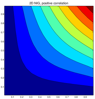
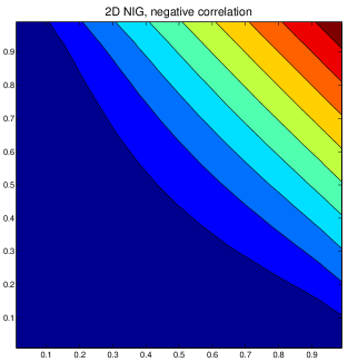
Figure 3.2. Contour plots of copulas for NIG, $t=1$.

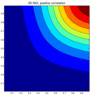
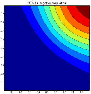
Figure 3.3. Contour plots of copulas for NIG, $t=\frac{1}{2}$.

4. Final remarks

We will not elaborate on the speed of Fourier methods compared with Monte Carlo methods in the multidimensional case; the interested reader is refered to Hurd and Zhou (2010) for a careful analysis. Moreover, Villiger (2007) provides recommendations on the efficient implementation of Fourier integrals using sparse grids in order to deal with the ‘curse of dimensionality’. Let us point out though that the computation of the copula function will be much quicker than the computation of the copula density, since the integrand in (2.2) decays much faster than the one in (2.7). One should think of the analogy to option prices and option Greeks again. Finally, it seems tempting to use these formulas for the computation of tail dependence coefficients. However, due to numerical instabilities at the limits, they did not yield any meaningful results.

References

- Barndorff-Nielsen (1998) O. E. Barndorff-Nielsen. Processes of normal inverse Gaussian type. Finance Stoch., 2:41–68, 1998.
- Blæsild (1981) P. Blæsild. The two-dimensional hyperbolic distribution and related distributions, with an application to Johannsen’s bean data. Biometrika, 68:251–263, 1981.
- Cuchiero et al. (2011) C. Cuchiero, D. Filipović, E. Mayerhofer, and J. Teichmann. Affine processes on positive semidefinite matrices. Ann. Appl. Probab., 21:397–463, 2011.
- Duffie et al. (2003) D. Duffie, D. Filipović, and W. Schachermayer. Affine processes and applications in finance. Ann. Appl. Probab., 13:984–1053, 2003.
- Eberlein and Madan (2010) E. Eberlein and D. Madan. On correlating Lévy processes. J. Risk, 13:3–16, 2010.
- Eberlein et al. (2010) E. Eberlein, K. Glau, and A. Papapantoleon. Analysis of Fourier transform valuation formulas and applications. Appl. Math. Finance, 17:211–240, 2010.
- Hurd and Zhou (2010) T. R. Hurd and Z. Zhou. A Fourier transform method for spread option pricing. SIAM J. Financial Math., 1:142–157, 2010.
- Jacod and Protter (2003) J. Jacod and P. Protter. Probability Essentials. Springer, 2nd edition, 2003.
- Kallsen and Tankov (2006) J. Kallsen and P. Tankov. Characterization of dependence of multidimensional Lévy processes using Lévy copulas. J. Multivariate Anal., 97:1551–1572, 2006.
- Kawai (2009) R. Kawai. A multivariate Lévy process model with linear correlation. Quant. Finance, 9:597–606, 2009.
- Khanna and Madan (2009) A. Khanna and D. Madan. Non Gaussian models of dependence in returns. Preprint, SSRN/1540875, 2009.
- Luciano and Schoutens (2006) E. Luciano and W. Schoutens. A multivariate jump-driven financial asset model. Quant. Finance, 6:385–402, 2006.
- Luciano and Semeraro (2010) E. Luciano and P. Semeraro. A generalized normal mean-variance mixture for return processes in finance. Int. J. Theor. Appl. Finance, 13:415–440, 2010.
- McNeil et al. (2005) A. McNeil, R. Frey, and P. Embrechts. Quantitative Risk Management: Concepts, Techniques and Tools. Princeton University Press, 2005.
- Muhle-Karbe et al. (2012) J. Muhle-Karbe, O. Pfaffel, and R. Stelzer. Option pricing in multivariate stochastic volatility models of OU type. SIAM J. Financial Math., 3:66–94, 2012.
- Rüschendorf (2009) L. Rüschendorf. On the distributional transform, Sklar’s theorem, and the empirical copula process. J. Statist. Plann. Inference, 139:3921–3927, 2009.
- Sato (1999) K. Sato. Lévy Processes and Infinitely Divisible Distributions. Cambridge University Press, 1999.
- Schmidt (2003) R. Schmidt. Dependencies of Extreme Events in Finance. PhD thesis, Univ. Ulm, 2003.
- v. Hammerstein (2011) E. A. v. Hammerstein. Generalized Hyperbolic Distributions: Theory and Applications to CDO Pricing. PhD thesis, Univ. Freiburg, 2011.
- Villiger (2007) S. Villiger. Basket option pricing on sparse grids using fast Fourier transforms. Master’s thesis, ETH Zürich, 2007.