Energy and Angular Momentum Storage in a Rotating Magnet

Abstract

We consider a cylindrical metallic magnet that is set into rotation about a horizontal axis by a falling mass. In such a system the magnetic field will cause a radial current which is non-solenoidal. This leads to charge accumulation and a partial attenuation of radial current. The magnetic field acting on the radially flowing current slows down the acceleration. Using newtonian dynamics we evaluate the angular velocity and displacement. We explicitly show that the electromagnetic angular momentum must be taken into consideration in order to account for the change in angular momentum due to the external torque on the system. Further the loss in potential energy of the falling mass can be accounted for only after taking into consideration the electrostatic energy and the Joule loss. We suggest that this example will be of pedagogical value to intermediate physics students. A version of this is scheduled to appear in American Journal of Physics 2011.

I Introduction

Introductory and intermediate treatments of electromagnetism usually shy away from a formal discussion of electromagnetic angular momentum and energy.hall92 ; serw94 ; gian00 Discussions if any are kept at a qualitative level. Specific examples involving forces and torques as well as the associated work done and the change in angular momentum are conspicuous by their absence. In a series of articles Gauthier has attempted to redress this lacuna.gaut82 ; gaut02

In one of his articles Gauthier considers a metallic cylindrical shell free to rotate about the horizontal axis.gaut02 A string wound around the shell with a mass attached to its free end causes it to rotate with acceleration. A charge is smeared on the shell making it analogous to a solenoid carrying an increasing time dependent current and associated magnetic flux. One can show from Faraday’s law that a retarding torque will act on the shell. This torque is of purely electromagnetic origin. Gauthier goes on to demonstrate in a pedagogically satisfying fashion that the system’s magnetic energy and electromagnetic momentum are stored at the expense of their mechanical counterparts.

In the present article we consider a cylindrical magnet free to rotate about the horizontal axis. We treat the magnetic field of the magnet to be constant and pointing along the axis. A string wound around the shell with a mass attached to its free end causes it to rotate with acceleration. We assume that the magnet is a good conductor and hence a radial current will be set up. The magnetic field will act on the radial current giving rise to a counter torque which will oppose the torque due to gravity.cylinder_inB The problem is complementary to Gauthier’s. Instead of Faraday’s law we need to invoke the Lorentz force, Gauss’s law and the equation of continuity. But the perspective is the same as Gauthier’s: an understanding of the problem involves a detailed consideration of the electromagnetic energy and angular momentum. We thus present another pedagogical example for an intermediate electromagnetic course.

II Dynamics of a rotating magnet

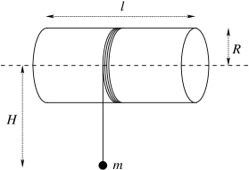
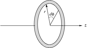
Figure 1: (a) Setup. (b) The cylindrical coordinate system. See text for details.

Consider a cylinder with moment of inertia $I$, radius $R$ and length $l$. Let mass $m$ be hung by a light thread wound on the surface of the cylinder. We adopt the cylindrical coordinate system {$r,\phi,z$} and unit vectors {$\hat{r},\hat{\phi},\hat{k}$} with $\hat{k}$ being the axis around which cylinder is free to rotate. Figure 1(a) illustrates the setup and Fig. 1(b) the cylindrical coordinate system we have adopted. When mass $m$ is released, the cylinder rotates with instantaneous angular velocity $\omega^{\prime}(t)\hat{k}$. We assume no slip condition $v=r\omega^{\prime}$. In that case Newton’s second law for rotational dynamics can be used to show that angular velocity of the cylinder is gaut02

$$\omega^{\prime}=\frac{\beta}{\tau_{1}^{2}}t,$$ (1)

where we have introduced a dimensionless constant

$$\beta=\dfrac{mR^{2}}{I+mR^{2}},$$ (2)

and a time constant

$$\dfrac{1}{\tau_{1}^{2}}=\dfrac{g}{R}.$$ (3)

We now replace the cylinder by a metallic cylindrical magnet in the setup. Let the conductivity of the cylinder be $\sigma$ and the magnetic field be uniform and $B\hat{k}$.cylinder_inB This is similar to the setup described by Gauthier gaut02 except that we have a solid cylindrical magnet instead of a non-magnetic charged cylindrical shell. As the magnet rotates due to the gravitational torque of the falling mass, the free charge in the rotating magnet experiences a radially outward Lorentz force. The magnetic field will act on this radial current and will produce a counter torque ($\tau_{em}$) which will oppose the torque due to gravity. The subscript indicates that the torque is of purely electromagnetic origin. We can write the equation of motion for the system as

$$mgR-\tau_{em}(t)=(I+mR^{2})\frac{d\omega}{dt}.$$ (4)

In what follows we will determine $\tau_{em}$ and solve the equation of motion.

Consider a free charge $q$ at a distance $r\ (r<R)$ from the axis of the cylinder rotating with angular velocity $\omega$. It is subjected to a radial Lorentz force $q\omega rB\hat{r}$. Recall that in literature the effect of this force is discussed in terms of motional emf. griffith ; galili06 From Ohm’s law this motion would lead to a current density $\vec{J}_{m}=\sigma\omega rB\hat{r}$. It is important to note that this current density is non-solenoidal

$$\vec{\nabla}.\vec{J}_{m}=\frac{1}{r}\frac{d}{dr}(rJ_{m})\neq 0$$

and hence charge must accumulate. This accumulating charge will give rise to a electric field ($\vec{E}_{a}$). Let $\rho(\vec{r},t)$ be the charge distribution due to accumulation. Associated with this $\rho(\vec{r},t)$ is an electric field which can be determined by Gauss’s law with the standard pill box construction in the magnet hall92

$$E_{a}=\frac{1}{\epsilon_{0}r}\int^{r}_{0}{\rho(r^{\prime},t)r^{\prime}dr^{\prime}}\ \ \ \ (r<R),$$

where we assume that the length of magnet $l\gg R$. Once again we use Ohm’s law to obtain $\vec{J}_{a}=\sigma E_{a}\hat{r}$. The resulting current density across the magnet is then

$$\vec{J}=\sigma\left(\omega rB+\frac{1}{\epsilon_{0}r}\int^{r}_{0}{\rho(r^{\prime},t)r^{\prime}dr^{\prime}}\right)\hat{r},$$ (5)

It consists of two terms: the first is due to the motional emf and second is due to charge accumulation. Next examine the divergence of current density

$$\vec{\nabla}.\vec{J}=\frac{1}{r}\frac{d}{dr}(rJ)=\sigma\left(2\omega B+\frac{1}{\epsilon_{0}}\rho(r,t)\right)$$

From equation of continuity

$$\vec{\nabla}.\vec{J}+\frac{\partial\rho}{\partial t}=0$$

we obtain

$$\frac{\partial\rho}{\partial t}+\frac{\sigma\rho}{\epsilon_{0}}=-2B\sigma\omega(t).$$ (6)

We assume that initially the cylinder is neutral ($\rho(\vec{r},t=0)=0$). Using this, Eq. (6) can be solved to yield

$$\rho(r,t)=-2B\sigma e^{-t/\tau_{2}}\int^{t}_{0}{\omega(t^{\prime})e^{t^{\prime}/\tau_{2}}dt^{\prime}},$$ (7)

where $\tau_{2}=\epsilon_{0}/\sigma$. The reader may have encountered $\tau_{2}$ earlier. When a lump of charge is deposited on a conductor, it spreads out in a very short time and with time constant $\tau_{2}$. Note that $\rho$ is independent of $r$. In order to maintain electrical neutrality there will be an accumulation of charges at the surface with the sign opposite to $\rho$. Hence

$$E_{a}=0\ \ \ \ \ \ \ \ (r>R).$$ (8)

Consider an annular element of radius $r<R$ in the cylinder (see Fig. 1). The force ($d\vec{F}$) on the annular element can be written as

$$d\vec{F} = 2\pi lrJd\vec{r}\times\vec{B}$$

$$= 2\pi lrJB(-\hat{\phi})dr$$

The associated torque ($d\vec{\tau}_{em}$) on the ring will be

$$d\vec{\tau}_{em}(t)=\vec{r}\times d\vec{F}=2\pi r^{2}lJB(-\hat{k})dr$$

The subscript indicates that torque is of electromagnetic origin. The net torque is obtained by straight forward integration

$$d\vec{\tau}_{em}(t)=\vec{r}\times d\vec{F}=2\pi r^{2}lJB(-\hat{k})dr.$$

Using the expressions for $J$ (Eq. (5)) and $\rho$ (Eq. (7)) one may obtain the net torque after straight forward integration

$$\tau_{em}(t)=\frac{\pi l\sigma B^{2}R^{4}}{2}\left(\omega(t)-\frac{1}{\tau_{2}}e^{-t/\tau_{2}}\int^{t}_{0}{\omega(t^{\prime})e^{t^{\prime}/\tau_{2}}dt^{\prime}}\right).$$ (9)

We pause to note that since the charge density is independent of $r$, the electric field from Gauss’s law will have a linear dependence on $r$. Ohm’s law implies that the current density would also be linearly dependent on $r$. It now remains to determine the time dependence. Differentiating above Eq. (4) with respect to $t$ gives

$$\frac{d^{2}\omega}{dt^{2}}=\frac{1}{(I+mR^{2})}\frac{d}{dt}\tau_{em}$$ (10)

Using Eq. (9)

$$\frac{d}{dt}\tau_{em}=\frac{\pi l\sigma B^{2}R^{4}}{2}\left(\frac{d\omega}{dt}-\frac{1}{\tau_{2}}\left(-\frac{1}{\tau_{2}}e^{-t/\tau_{2}}\int^{t}_{0}{\omega(t^{\prime})e^{t^{\prime}/\tau_{2}}dt^{\prime}}+\omega(t)\right)\right)$$ (11)

The integral term on the r.h.s of Eq. (11) can be eliminated using Eqs. (9) and (4). Hence we may rewrite Eq. (10) as

$$\frac{d^{2}\omega}{dt^{2}}+\left(\frac{\pi l\sigma B^{2}R^{4}}{2(I+mR^{2})}+\frac{1}{\tau_{2}}\right)\frac{d\omega}{dt}=\frac{mgR}{\tau_{2}(I+mR^{2})}.$$ (12)

We define a time constant

$$\frac{1}{\tau_{3}}=\frac{\pi lB^{2}\sigma R^{4}}{2(I+mR^{2})},$$ (13)

and an effective time constant

$$\frac{1}{\tau_{e}}=\frac{1}{\tau_{2}}+\frac{1}{\tau_{3}}.$$

One can solve Eq. (12) using initial condition $\omega(t=0)=0$ and $d\omega/dt=\beta/\tau_{1}^{2}$ to obtain

$$\omega(t)=\frac{\beta}{\tau_{1}^{2}}t-\frac{\beta\tau_{e}}{\tau_{1}^{2}\tau_{3}}f(t)$$ (14)

$$\mbox{where}\ \ \ f(t)=t-\tau_{e}\left(1-e^{-t/\tau_{e}}\right)$$ (15)

Note that the first term in Eq. (14) is same as Eq. (2). Also

$$f(t)>0$$

This indicates that the angular velocity in case of magnet is never greater than in the case of non-magnetic solid cylinder. We consider two limits of the Eq. (14)

$$\omega(t\ll\tau_{e}) \approx \frac{\beta}{\tau_{1}^{2}}t-\frac{\beta}{2\tau_{1}^{2}\tau_{3}}t^{2}$$ (16)

$$\omega(t\gg\tau_{e}) \approx \frac{\beta\tau_{e}}{\tau_{1}^{2}\tau_{2}}t$$ (17)

$$< \frac{\beta}{\tau_{1}^{2}}t=\omega^{\prime}$$ (18)

This shows that the effect of the metallic magnet is to decrease the angular velocity from the non-magnetic value ($\omega^{\prime}$). A straightforward integration also yields the angular distance traversed

$$\phi(t)=\frac{\beta\tau_{e}^{2}}{\tau_{1}^{2}\tau_{3}}f(t)+\frac{\beta\tau_{e}}{2\tau_{1}^{2}\tau_{2}}t^{2}$$ (19)

Once again we note the limiting cases

$$\phi(t\ll\tau_{e}) = \frac{\beta}{2\tau_{1}^{2}}t^{2}$$

$$\phi(t\gg\tau_{e}) = \frac{\beta\tau_{e}^{2}}{\tau_{1}^{2}\tau_{3}}t+\frac{\beta\tau_{e}}{2\tau_{1}^{2}\tau_{2}}t^{2}$$

$$< \frac{\beta}{2\tau_{1}^{2}}t^{2}$$

which indicates that the magnetic field slows down the rotation. Using Eq. (14) in Eq. (7) and integrating we obtain charge density

$$\rho(t)=\frac{-2B\sigma\beta\tau_{e}}{\tau_{1}^{2}}f(t).$$ (20)

We remind the reader that $f(t)>0$ and hence charge density is negative.chargedensity Also, as stated earlier, a compensating positive charge collects on the surface so that the magnet is on the whole neutral. We have already pointed out that $\rho$ is independent of $r$ and therefore the electric field is

$$\vec{E}_{a}=\frac{\rho(t)r}{2\epsilon_{0}}\hat{r} = -\frac{B\beta\tau_{e}r}{\tau_{1}^{2}\tau_{2}}f(t)\hat{r}\ \ \ \ \ (r<R),$$ (21)

$$= 0\ \ \ \ \ \ \ \ \ \ \ \ \ \ \ \ \ \ \ \ \ \ (r>R).$$ (22)

We then calculate the total current density

$$\vec{J}=\frac{\sigma rB\beta}{\tau_{1}^{2}}\left(t-f(t)\right)\hat{r}.$$ (23)

while the net electromagnetic torque on the system is

$$\tau_{em}=\frac{\pi\epsilon_{0}lB^{2}R^{4}\beta}{2\tau_{1}^{2}\tau_{2}}(t-f(t)).$$ (24)

We pause to comment briefly on the time dependence of above quantities. Note that $t-f(t)=\tau_{e}(1-e^{-t/\tau_{e}})$. As physically expected both the current density and electromagnetic torque are initially zero and they both saturate to a constant value at large times.

III verification of angular momentum

The electromagnetic angular momentum ($L_{em}$) is defined in terms of electric and magnetic field.griffith In our case we have

$$\vec{L}_{em}=\int^{R}_{0}{\epsilon_{0}}\vec{r^{\prime}}\times(\vec{E}_{a}\times\vec{B})\,2\pi r^{\prime}ldr^{\prime}$$ (25)

Using the expression for electric field due to the charge accumulation (Eq. (21)) we have,

$$\vec{L}_{em} = -\frac{\epsilon_{0}B^{2}\beta\tau_{e}2\pi l}{{\tau_{1}}^{2}\tau_{2}}f(t)\int^{R}_{0}r^{\prime}\hat{r}\times(r^{\prime}\hat{r}\times\hat{k})r^{\prime}dr^{\prime}$$ (26)

$$= \frac{\epsilon_{0}B^{2}\beta\tau_{e}2\pi l}{{\tau_{1}}^{2}\tau_{2}}f(t)\int^{R}_{0}r^{\prime 3}dr^{\prime}\hat{k}$$

$$= \frac{\epsilon_{0}B^{2}\beta\tau_{e}\pi lR^{4}}{2{\tau_{1}}^{2}\tau_{2}}f(t)\hat{k}$$

Since $f(t)$ is always positive it means that some angular momentum is transferred to the electromagnetic field and consequently the mechanical angular momentum is diminished. One can check that differentiating the above equation for $L_{em}$, we will obtain precisely Eq. (24) for electromagnetic torque. The mechanical angular momentum of the system is

$$\vec{L}_{m}=(I+mR^{2})\omega\hat{k}=(I+mR^{2})\left(\frac{\beta}{\tau_{1}^{2}}t-\frac{\beta\tau_{e}}{\tau_{1}^{2}\tau_{3}}f(t)\right)\hat{k}.$$ (27)

Adding Eqs. (26) and (27), we see that the terms associated with $f(t)$ cancel and lead to the expression

$$\vec{L}_{em}+\vec{L}_{m}=mgRt\hat{k}.$$ (28)

as it should, being the change in angular momentum due to the external torque on the system.

IV Energy Balance

As the hanging mass drops a distance $H$, the loss in potential energy is

$$U=mgH=mgR\phi(t),$$ (29)

where $\phi(t)$ is given by Eq. (19). At first sight it may seem that this potential energy is distributed into two channels : (i) gain in kinetic energy of system (mass+cylinder) and (ii) electrical energy stored in the system. Let us evaluate the contributions of these two channels.

The total kinetic energy after the hanging mass has dropped a distance $H=R\phi(t)$ is

$$K = \frac{1}{2}I\omega^{2}+\frac{1}{2}mv^{2}$$ (30)

$$= \frac{I+mR^{2}}{2}\omega^{2}.$$

where $v$ is the linear speed of the falling mass and $\omega$ is given by Eq. (14). On the other hand the stored electrical energy ($U_{e}$) is

$$U_{e} = \frac{\epsilon_{0}}{2}\int^{R}_{0}{E_{a}^{2}\,2\pi lr^{\prime}\,dr^{\prime}}$$ (31)

$$= \frac{\epsilon_{0}\pi lB^{2}\beta^{2}\tau_{e}^{2}R^{4}}{4\tau_{1}^{4}\tau_{2}^{2}}f^{2}(t).$$ (32)

Note that the integration is up to $R$ only (See Eq. (8)). However adding Eqs. (30) and (32) yields

$$U-(K+U_{e})=(I+mR^{2})\frac{\beta^{2}\tau_{e}}{2\tau_{1}^{4}\tau_{3}}\left[2\tau_{e}f(t)-\left(f(t)-t\right)^{2}\right].$$ (33)

The right hand side is evidently not zero. We need to evaluate the Joule loss. This is given by

$$U_{J} = \frac{1}{\sigma}\int^{t}_{0}{\int^{R}_{0}{J^{2}\,2\pi lr^{\prime}\,dr^{\prime}dt^{\prime}}},$$ (34)

where the current density is given by Eq. (23). The heat loss in a conductor is due to the collision of the charge carriers with the surrounding atoms. The collisions result in the dissipation of kinetic energy of the charge carriers in the form of heat. This motion of charge carriers arises from two mutually opposing processes: (i) the electric field $E_{a}$ given by Eq. (21) and (ii) the Lorentz force. Note that in the evaluation of angular momentum (Eq. (25)) we considered only electric field ($E_{a}$). The point to appreciate is that in the case of energy conservation we need to also consider the Lorentz force since it results in the motion of charge with consequent loss in kinetic energy due to collisions. Substituting the current density from Eq. (23) and using Eq. (15), we obtain

$$U_{J} = \frac{\sigma B^{2}\beta^{2}\pi l\tau_{e}^{2}R^{4}}{2\tau_{1}^{4}}\int^{t}_{0}\tau^{2}_{e}(1-e^{-t^{\prime}/\tau_{e}})^{2}dt^{\prime}.$$ (35)

$U_{J}$ can be evaluated by lengthy and straightforward integration (See Appendix for detailed derivation of $U_{J}$). It yields precisely the r.h.s. of Eq. (33). Thus

$$mgH=K+U_{e}+U_{J}.$$

V Discussion

Let us recapitulate the physical processes which are involved. The magnet rotates due to the gravitational torque of the falling mass. The free charge in the rotating magnet experiences a radially outward force. The resulting radial current is non-solenoidal. This implies that charge will accumulate. The electric field due to the charge accumulation will retard the radial motion of free charge. The resulting diminished radial current will nevertheless give rise to a counter-torque which is of patently electromagnetic origin. Newton’s second law can be applied to derive the angular velocity and angular acceleration. Next, we demonstrate by detailed bookkeeping that energy and angular momentum are properly accounted for.

One may get a perspective on the problem by obtaining order of magnitude estimates of time constants involved. Let us take the radius of the magnet $R$= 0.1 m, length $l$ = 1 m, density same as that of iron (7800 kg$\cdot$m^-3), conductivity $\sigma=10^{7}$ S$\cdot$m^-1 and magnetic field $B$ to be 1 T. Let the falling mass be 10 kg. This yields $\tau_{1}\approx 10^{-1}\,\mbox{s},\ \tau_{2}\approx 10^{-18}\,\mbox{s},\ \tau_{3}\approx 10^{-3}\,\mbox{s}$ and $\tau_{e}\approx 10^{-18}\,\mbox{s}$. Note that $\tau_{e}\cong\tau_{2}$. When one uses these numbers then one finds that current density is very small and of order 10^-12 A$\cdot$m^-2. Thus the motion of the charges will have a negligible effect on the magnetic field. The observable effects are possible if the magnetic field is unusually large as happens in magnetars with magnetic field of gigateslas.macd00 However it is important to realise that howsoever small the effects due to magnetic field may be they are crucial in accounting for the angular momentum and energy balance.

*

Appendix A

We substitute the expression for current density from Eq. (23) into Eq. (34) and get

$$U_{J} = \frac{\sigma B^{2}\beta^{2}2\pi l\tau_{e}^{2}}{\tau_{1}^{4}}\int^{R}_{0}r^{\prime 3}dr^{\prime}\int^{t}_{0}\left(t^{\prime}-f(t^{\prime})\right)^{2}dt^{\prime}$$ (36)

The integrand associated with the $t$ variable can be simplified with the help of Eq. (15) for $f(t)$ and this yields

$$U_{J} = \frac{\sigma B^{2}\beta^{2}\pi l\tau_{e}^{2}R^{4}}{2\tau_{1}^{4}}\int^{t}_{0}\tau^{2}_{e}(1-e^{-t^{\prime}/\tau_{e}})^{2}dt^{\prime}$$

Expanding and integrating the squared term and using the time constant $\tau_{3}$ (Eq. (13))

$$U_{J} = (I+mR^{2})\frac{\beta^{2}\tau_{e}^{2}}{\tau_{1}^{4}\tau_{3}}\left(t+\frac{\tau_{e}}{2}(1-e^{-2t/\tau_{e}})-2\tau_{e}(1-e^{-t/\tau_{e}})\right)$$

Using Eq. (15) once again

$$U_{J} = (I+mR^{2})\frac{\beta^{2}\tau_{e}^{2}}{\tau_{1}^{4}\tau_{3}}\left(t+\frac{t-f(t)}{2}\left(2-\frac{t-f(t)}{\tau_{e}}\right)-2(t-f(t))\right)$$ (37)

$$= (I+mR^{2})\frac{\beta^{2}\tau_{e}^{2}}{\tau_{1}^{4}\tau_{3}}\left(f(t)-\frac{\left(t-f(t)\right)^{2}}{2\tau_{e}}\right)$$

Equation (37) is precisely the r.h.s. of Eq. (33).

References

- (1) D. Halliday, R. Resnick, and K. S. Krane, Physics, 4th ed. (Wiley, New York, 1992), Vol. 2.
- (2) R. A. Serway, Principles of Physics (Saunders, New York, 1994).
- (3) D. C. Giancoli, Physics for Scientists and Engineers (Prentice-Hall, New Jersey, 2000).
- (4) N. Gauthier, “A Newton Faraday approach to electromagnetic energy and angular momentum storage in an electromechanical system,” Am. J. Phys., 70, 1034-1038 (2002).
- (5) N. Gauthier and H. D. Wiederick, “Note on the magnetic energy density,” Am. J. Phys. 50, 758-759 (1982).
- (6) Instead of a magnet we can also consider a long metallic cylinder placed in a uniform magnetic field directed along the axis of the cylinder.
- (7) Griffiths D., Introduction to Electrodynamics, 2nd ed. (Prentice-Hall, New Delhi, 1989).
- (8) Galili I., Kaplan D., Lehavi Y., “Teaching Faraday’s law of electromagnetic induction in an introductory physics course,” Am. J. Phy., 74, 337-343 (2006).
- (9) Note that the increase of charge with time cannot happen indefinitely. We have assumed in our model that conductivity is constant.
- (10) Kirk T. McDonald, “Magnetars,” Am. J. Phy., 68, 775 (2000).