A tilted interference filter in a converging beam

Abstract

Context. Narrow-band interference filters can be tuned toward shorter wavelengths by tilting them from the perpendicular to the optical axis. This can be used as a cheap alternative to real tunable filters, such as Fabry-Pérot interferometers and Lyot filters. At the Swedish 1-meter Solar Telescope, such a setup is used to scan through the blue wing of the Ca ii H line. Because the filter is mounted in a converging beam, the incident angle varies over the pupil, which causes a variation of the transmission over the pupil, different for each wavelength within the passband. This causes broadening of the filter transmission profile and degradation of the image quality.

Aims. We want to characterize the properties of our filter, at normal incidence as well as at different tilt angles. Knowing the broadened profile is important for the interpretation of the solar images. Compensating the images for the degrading effects will improve the resolution and remove one source of image contrast degradation. In particular, we need to solve the latter problem for images that are also compensated for blurring caused by atmospheric turbulence.

Methods. We simulate the process of image formation through a tilted interference filter in order to understand the effects. We test the hypothesis that they are separable from the effects of wavefront aberrations for the purpose of image deconvolution. We measure the filter transmission profile and the degrading PSF from calibration data.

Results. We find that the filter transmission profile differs significantly from the specifications. We demonstrate how to compensate for the image-degrading effects. Because the filter tilt effects indeed appear to be separable from wavefront aberrations in a useful way, this can be done in a final deconvolution, after standard image restoration with Multi-Frame Blind Deconvolution/Phase Diversity based methods. We illustrate the technique with real data.

1 Introduction

Narrowband (NB) interference filters can be tuned in wavelength by varying the incident angle. This is often used to allow for filter manufacturing margins by specifying the peak to the red of the wanted wavelength and then mounting the filter at a small angle to compensate. At the Swedish 1-m Solar Telescope (SST; Scharmer et al. 2003a), the effect is used for scanning through the blue wing of the Ca ii H line by use of a narrow-band (NB) filter mounted on a motor-controlled rotation stage. The tuning is possible because the filter cavity is geometrically wider for a ray intersecting with the filter at an angle from normal incidence.

However, even when the filter is mounted with no tilt with respect to the optical axis, rays arrive at a variety of angles. This has consequences for the spectral resolution as well as for the spatial resolution (Beckers 1998). Depending on the optical configuration, the spread in incident angles may cause a broadening of the transmission profile or variations in central wavelength over the field of view (FOV) or both. A problem related to the broadening is that the resolution suffers in telescopes that operate near the diffraction limit. The amplitude of the pupil transmission coefficient, as seen through the filter, is apodized by an amount that varies with the wavelength. Beckers evaluated the resolution effects of a Fabry-Pérot interferometer (FPI) used in the pupil plane of a telecentric setup. von der Lühe & Kentischer (2000) included also the phase of the field transmission in their analysis. Scharmer (2006) showed that the dominating part of the phase effects is in the form of a wavelength independent, quadratic pupil phase that can be compensated with a simple re-focusing of the detector.

The effects investigated by the authors cited above are greater the narrower the bandpass, making this a problem primarily for FPIs with FWHMs in the picometer range. However, as we will demonstrate in this paper, there are significant effects also for filters with a FWHM of $\sim$0.1 nm when tilted by a few degrees. We analyze a NB double-cavity filter, mounted in a converging beam at an angle from the optical axis. We show that the resulting degradation of image quality can be compensated for by deconvolution and that images degraded by this effect as well as atmospheric seeing can be significantly improved. The effect is apparently separable from phase aberrations in the sense that they can be modeled as separate transfer functions, to be applied in sequence. This is beneficial for wavefront sensing with the Multi-Frame Blind Deconvolution/Joint Phase Diverse Speckle (MFBD/JPDS) formalism of Löfdahl (2002).

We illustrate the technique with images from the SST recorded through a Ca ii H filter mounted on a computer controlled rotating stage. We use simulations of such data to illustrate the separability of the apodisation effects and phase aberrations. Appropriate and sufficient information needed to compensate for the image degradation can be obtained by calibration using pinhole images.

2 Theory and notation

2.1 Tilted cavities

In order to understand what happens when we tilt a filter, we begin by deriving the transmission coefficient for the electric field. The matrix formalism described by Klein & Furtak (1986, Sect. 5.4) implements multiple reflections and transmissions in both directions through many different layers. Assume light incident on a stack of $N$ layers from the left. We define the column vectors

$$\mathbf{E}_{j}=\left[\begin{array}[]{c}E_{\text{L}j}\\ E_{\text{R}j}\end{array}\right]\qquad\text{and}\qquad\mathbf{E}^{\prime}_{j}=\left[\begin{array}[]{c}E^{\prime}_{\text{L}j}\\ E^{\prime}_{\text{R}j}\end{array}\right],$$ (1)

where $\mathbf{E}_{j}$ represents the electric field on the left side of layer $j$ and $\mathbf{E}^{\prime}_{j}$ the field on the right side of the same layer. Indices L and R denote field moving to the left and right, respectively.

The relationship between the field in the incident medium and the field in the final medium can then be written as

$$\mathbf{E}^{\prime}_{1}=\mathbf{S}_{1N}\mathbf{E}_{N},$$ (2)

with the stack matrix

$$\mathbf{S}_{1N}=\left[\begin{array}[]{cc}S_{11}&S_{12}\\ S_{21}&S_{22}\\ \end{array}\right]=\mathbf{H}_{12}\mathbf{L}_{2}\cdots\mathbf{L}_{N-1}\mathbf{H}_{N-1,N}.$$ (3)

The interface transition matrix $\mathbf{H}_{ij}$ and the layer matrix $\mathbf{L}_{j}$ are defined as

$$\mathbf{H}_{ij}=\frac{1}{\tau_{ij}}\left[\begin{array}[]{cc}1&\rho_{ij}\\ \rho_{ij}&1\\ \end{array}\right]\qquad\text{and}\qquad\mathbf{L}_{i}=\left[\begin{array}[]{cc}e^{-\text{i}\beta_{j}}&0\\ 0&e^{\text{i}\beta_{j}}\\ \end{array}\right],$$ (4)

repectively, where $\tau_{ij}$ and $\rho_{ij}$ are the transmission and reflection coefficients, respectively, of the interface between medium $i$ and medium $j$, and

$$\beta_{j}=\frac{4\pi}{\lambda}n_{j}h_{j}\cos\alpha_{j}.$$ (5)

Here $n_{j}$ is the refractive index of medium $j$, $h_{j}$ is the geometrical thickness of the cavity, and $\alpha_{j}$ is the angle of the ray from the interface surface normal within medium $j$. Using these definitions and the boundary condition $E_{\text{L}N}=0$ (in the final medium there is no field moving to the left), the transmission coefficient of the stack can be written as

$$\tau=\frac{E_{\text{R}N}}{E^{\prime}_{\text{R}1}}=\frac{1}{S_{22}}.$$ (6)

Applying this formalism to a single cavity with index $n_{2}$ between media of index $n_{1}=n_{N}$, we get

$$\tau_{\text{sc}}=\frac{\tau_{12}\tau_{21}e^{-\text{i}\beta_{2}}}{1-\rho^{2}_{12}e^{-\text{i}2\beta_{2}}}.$$ (7)

If $n_{2}$, $h_{2}$, $d_{2}$, $\tau_{12}$, $\tau_{21}$, $\rho_{12}$, and $\rho_{12}$ are known, like for a FPI, this expression can be used to calculate the transmission of the cavity for any incident angle. However, manufacturers of dielectric filters usually only disclose the intensity transmittance ($T=|\tau|^{2}$) at normal incidence.

The transmission coefficient is a function of the wavelength as well as the incident angle through $\beta_{2}$. When the angle changes, the wavelength needed to keep $\beta_{2}$ (and thereby $\tau$) constant also changes. The effect of changing the angle is therefore to shift the transmission profile in wavelength. With the assumption of small angles, repeated application of Snell’s law, and trivial algebra, the well known (e.g., Smith 1990, chapter 7) expression

$$\lambda^{\prime}=\lambda\sqrt{1-\left(\frac{n_{1}}{n_{2}}\sin\alpha\right)^{2}},$$ (8)

can be derived, where $\lambda^{\prime}$ is the shifted wavelength and we define $\alpha=\alpha_{1}$.

With double cavities we get

$$\tau_{\text{dc}}=\frac{\tau_{12}\tau_{23}\tau_{34}\cdot e^{-\text{i}\overline{\beta}}}{1+\overline{\rho}^{2}e^{-\text{i}2\overline{\beta}}-\rho_{23}\rho_{34}e^{-\text{i}2\beta_{2}}-\rho_{12}\rho_{23}e^{-\text{i}2\beta_{3}}},$$ (9)

where we have defined $\overline{\beta}=(\beta_{2}+\beta_{3})$, and $\overline{\rho}^{2}=\rho_{12}\rho_{23}+\rho_{23}\rho_{34}+\rho_{12}\rho_{34}$. The numerator shifts as given by the shift of $\overline{\beta}$, which means it behaves like the transmission profile for a single cavity and an “effective” refractive index $n$ can be defined. The last two terms in the denominator shift differently but the behavior of the numerator should dominate.

2.2 Pupil transmission in a converging beam

For a piece of optics in a converging beam, the incident angle of a light ray varies with the orientation of the optics relative to the optical axis, but also with the location within the pupil that the ray emanates from. As we have seen, the transmission coefficient $\tau(\lambda)$ of an interference filter varies with the incident angle, so that it is shifted toward shorter wavelengths.

For incoming light with a wavelength $\lambda$, the generalized pupil function may be written as

$$P(x_{\mathrm{p}},y_{\mathrm{p}},\lambda;\phi,\theta)=\tau_{\text{p}}(x_{\mathrm{p}},y_{\mathrm{p}},\lambda;\theta)\,A(x_{\mathrm{p}},y_{\mathrm{p}})\exp\{\mathrm{i}\phi(x_{\mathrm{p}},y_{\mathrm{p}})\},$$ (10)

where $(x_{\mathrm{p}},y_{\mathrm{p}})$ are coordinates within the pupil (here normalized to unit diameter), $A$ is a binary function representing the geometrical shape of the pupil stop, $\mathrm{i}$ is the imaginary unit, $\theta$ is the tilt angle of the filter around the $y$ axis, and $\phi$ is the phase aberrations from the atmosphere, the telescope, and any other optics, independent of $\lambda$. The filter’s complex transmission coefficient as seen through the pupil can be written as

$$\tau_{\text{p}}(x_{\mathrm{p}},y_{\mathrm{p}},\lambda;\theta)=\tau_{\text{f}}\bigl{(}\lambda^{\prime}(\lambda,\alpha(x_{\mathrm{p}},y_{\mathrm{p}};\theta))\bigr{)},$$ (11)

where $\tau_{\text{f}}$ is the normal incidence complex transmission coefficient of the electric field vector through the filter, and $\lambda^{\prime}$ is the shifted wavelength given by Eq. (8). In Appendix A we derive an expression for the incident angle, $\alpha$, on a tilted filter in a converging beam. With the added assumption that the detector is small, we can write it as

$$\alpha(x_{\mathrm{p}},y_{\mathrm{p}};\theta)=\arccos\left(\frac{F\cos\theta+x_{\mathrm{p}}\sin\theta}{(F^{2}+x_{\mathrm{p}}^{2}+y_{\mathrm{p}}^{2})^{1/2}}\right),$$ (12)

where $F$ is the effective F-ratio.

2.3 Point spread function and optical transfer function

Because of Eq. (8), we know that NB interference filters can be tuned by tilting the filter normal from the optical axis. In addition to the desired change in peak wavelength, the tilting has consequences for the width of the profile and for the shape of the PSF because of Eq. (12).

We model the image formation process as a space-invariant (valid for sufficiently small sub-fields) convolution between an unknown object $f$ and a point spread function $s_{k}$, the Fourier transforms of which are $F$ and $S_{k}$, where the index $k$ corresponds to a particular data frame. An additive Gaussian noise term $n_{k}$ is assumed. The Fourier transform $D_{k}$ of the observed image $d_{k}$ is then related to $F$, $S_{k}$ and $N_{k}$ via

$$D_{k}=FS_{k}+N_{k}.$$ (13)

These quantities are all functions of the spatial frequency coordinates $u$ and $v$ but to ease the notation, we will not write them out. The assumption of additive Gaussian noise leads to a simple Maximum Likelihood expression for an estimate of the object through multi-frame deconvolution,

$$\hat{F}=H\sum_{k}D_{k}S_{k}^{*}\biggm{/}\sum_{k}|S_{k}|^{2},$$ (14)

where $H$ is a low-pass noise filter and $*$ used as a superscript denotes the complex conjugate.

Because the profiles are shifted by different amounts over the pupil, the transmittance of light of different wavelengths through the pupil is not uniform. At every wavelength within the broadened passband, the transmittance of light from different parts of the pupil corresponds to different parts of the normal-incidence filter profile. Because light interferes only with light of the same wavelength, $S_{k}$ cannot be calculated with the usual quasi-monochromatic assumption. Instead, it must be modeled as the integrated, monochromatic contributions from the different wavelengths within the passband. With a discrete approximation, we can write

$$S_{k}=S(\phi_{k},\theta)=\delta\lambda\sum_{\ell}^{L}\operatorname{\mathfrak{F}}\left\{\left|\operatorname{\mathfrak{F}}^{-1}P(x_{\mathrm{p}},y_{\mathrm{p}},\lambda_{\ell};\phi_{k},\theta)\right|^{2}\right\},$$ (15)

where the summation is performed over $L$ samples distributed over the broadened passband.

What we would really want is for $S_{k}$ to be separable in two parts: 1) the usual OTF, including the pupil geometry, the atmospheric wavefront, as well as any other wavefront components introduced in the optics, and 2) another transfer function, compensating for the filter tilt effects. We would like to write

$$S(\phi_{k},\theta)\approx S_{\text{wf}}(\phi_{k})\cdot S_{\text{tilt}}(\theta),$$ (16)

where

$$S_{\text{wf}}(\phi)=\operatorname{\mathfrak{F}}\left\{\left|\operatorname{\mathfrak{F}}^{-1}A(x_{\mathrm{p}},y_{\mathrm{p}})\exp\{\mathrm{i}\phi(x_{\mathrm{p}},y_{\mathrm{p}})\}\right|^{2}\right\}$$ (17)

and

$$S_{\text{tilt}}(\theta)=\frac{1}{S_{0}}\delta\lambda\sum_{\ell}^{L}S_{\text{mono}}(\lambda_{\ell},\theta),$$ (18)

where we define the monochromatic tilt OTF as

$$S_{\text{mono}}(\lambda,\theta)=\operatorname{\mathfrak{F}}\left\{\left|\operatorname{\mathfrak{F}}^{-1}P(x_{\mathrm{p}},y_{\mathrm{p}};\lambda,0,\theta)\right|^{2}\right\}.$$ (19)

In the expression for $S_{\text{tilt}}$, we choose to include the pupil geometry and then divide it away as the diffraction limited MTF, $S_{0}=S_{\text{wf}}(0)$. This way it becomes natural not to define $\tau_{\text{p}}$ outside of the pupil. For simplicity of notation, and for the purpose of this discussion, we incorporate also any intentional phase diversity (PD) focus contribution in $\phi_{k}$.

We explore this separability in Sect. 3.3 below. The advantages with separability, for our purposes, is that the correction can be applied after restoration of the images for atmospheric turbulence effects, i.e., MFBD-based methods or speckle interferometry. And, since we assume the variation over the field of view is negligible, it can be done for the entire FOV in a single operation instead of by subfields like for the anisoplanatic atmosphere.

3 A 0.1 nm wide Ca ii H 396.9 nm filter

3.1 Filter properties

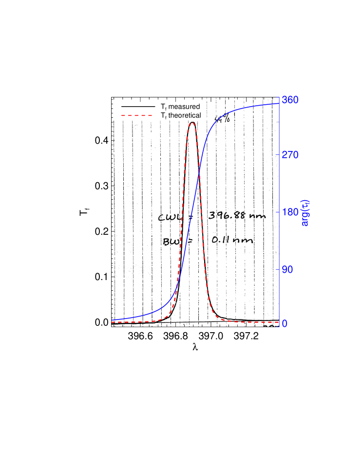
Figure 1: Filter profiles for normal incidence on the Ca ii H filter. Solid black: Transmittance, $T_{\text{f}}(\lambda)$, measured by the manufacturer before delivery of the filter; Dashed red: theoretical transmittance; Blue: theoretical transmission phase, $\arg(\tau_{\text{f}}(\lambda))$.

As the specific case, motivating this research, we discuss a Ca ii H filter, regularly used at the SST. The filter, manufactured by Barr Associates, Inc., was delivered in August 2000. The coating parameters are not public so we cannot calculate $\tau_{\text{f}}$ but along with the filter we got the measurements shown in Fig. 1. The central wavelength was specified to $\lambda_{\mathrm{c}}=396.88$ nm, the peak transmittance, $\max T_{\text{f}}$, to 44%, and the FWHM to 0.11 nm (at $23\degr$C and normal incidence).

In order to use Eq. (8), we need the effective refractive index. Rouppe van der Voort (2002, page 26) contacted the manufacturer after the filter was delivered and got the value $n=1.596$. Because we wanted to explore the effects of the phase, Potter (2004) later provided some design data: the phase of the filter transmission coefficient, $\arg\{\tau_{\text{f}}(\lambda)\}$, as well as the curve form of the transmittance profile in digital form, see the red and blue curves in Fig. 1. The wavelength range for both quantities is $394.9\text{ nm}\leq\lambda\leq 398.9\text{ nm}$. We show here the central part, rescaled to the measured peak transmittance of 44%.

The light beam from the telescope forms a pupil image, where our adaptive optics (Scharmer et al. 2003b) deformable mirror is mounted. From there, the beam is re-imaged by a field lens with a focal length of $\sim$1.5 m, making a F/46 beam. As seen from the pupil image, through the re-imaging lens, the 7 mm center to corner distance of our 10 mm by 10 mm detector corresponds to an angular size of $0.007/1.5$ rad or 0$\aas@@fstack{\circ}$27. As we will see, angles of this size has negligible impact so we are justified in ignoring variations over the FOV. The image scale, 0$\aas@@fstack{\prime\prime}$034/pixel, made by the re-imaging lens was established by observations of the Venus transit in 2004 (Kiselman 2008).

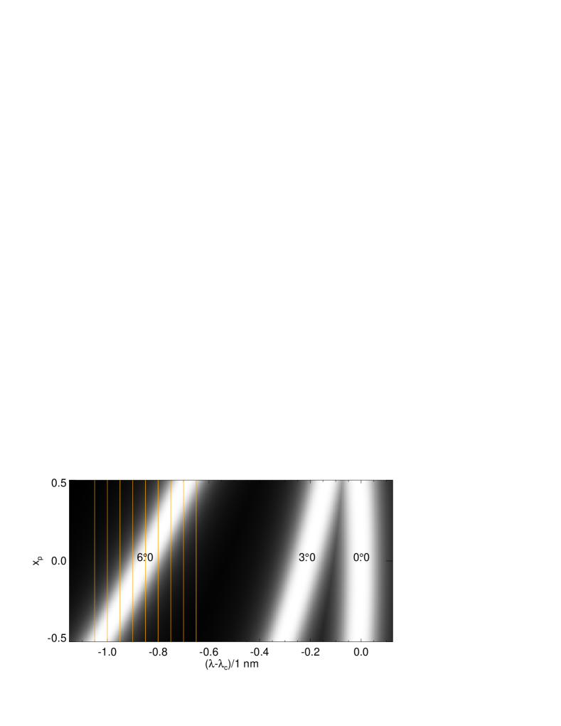
(a)

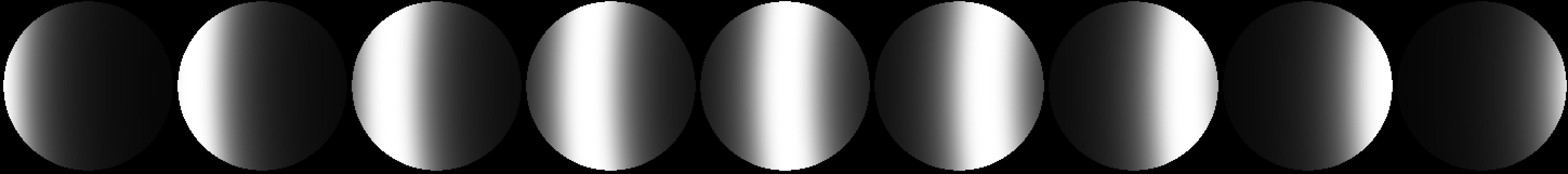
(b)

(c)

Figure 2: The transmission coefficient, $\tau_{\text{p}}$, profile data cube, calculated from the manufacturer’s theoretical profiles by use of Eqs. (10)–(12). LABEL:sub@fig:barr_transmissionx The modulus for $y_{\mathrm{p}}=0$, $|\tau_{\text{p}}(x_{\mathrm{p}},0,\lambda;\theta)|$, superimposed for $\theta=0\degr$, 3°, and 6° as labeled. LABEL:sub@fig:barr_transmissionP The pupil apodisations, $|\tau_{\text{p}}(x_{\mathrm{p}},y_{\mathrm{p}},\lambda_{\ell};6\degr)|$, sampled at the wavelengths $\lambda_{\ell}$ indicated with the orange lines in LABEL:sub@fig:barr_transmissionx. LABEL:sub@fig:barr_phaseP The corresponding pupil phases, $\arg\{\tau_{\text{p}}(x_{\mathrm{p}},y_{\mathrm{p}},\lambda_{\ell};6\degr)\}$.

The pupil apodisations vary with tilt angle, which is illustrated in Fig. 2. Increasing the angle moves the passband from the Ca ii H line core (formed in the solar chromosphere) toward the blue wing (formed in the photosphere). In the axis corresponding to the tilt direction, the transmittance profile peak position varies over the pupil (Fig. 2a). In the perpendicular direction, the peak position varies only slightly with distance from the center of the pupil. Sample pupil apodisations for one of the tilt angles are shown in Fig. 2b. Because of the angles of the transmittance ridges in Fig. 2a, larger tilt angles result in narrower apodisations over the pupil for each wavelength. For 0$\aas@@fstack{\circ}$0, the transmittance varies with wavelength, but with small variations within the pupil. For larger tilt angles, the apodisation function looks more and more like a band sweeping across the pupil.

The transmittance phase, $\arg(\tau_{\text{f}})$, has an approximately linear gradient where the modulus, $|\tau_{\text{f}}|$, has its peak, see Fig. 1. The phase profiles are shifted the same way as the transmittance profiles, so the phase gradient peaks at the same location in the pupil as the transmittance, see Figs. 2b and 2c.

3.2 Profiles

Integrating over the pupil results in broadened profiles, as noted by Beckers (1998), because of the varying shifts in the $x_{\mathrm{p}}$ direction. For our filter, $\theta=0\aas@@fstack{\circ}0$ results in a transmission profile that is virtually identical to the normal incidence profile but for angles of a few degrees, the broadening is significant, see the broadening as calculated for the manufacturer’s profile in Fig. 3.

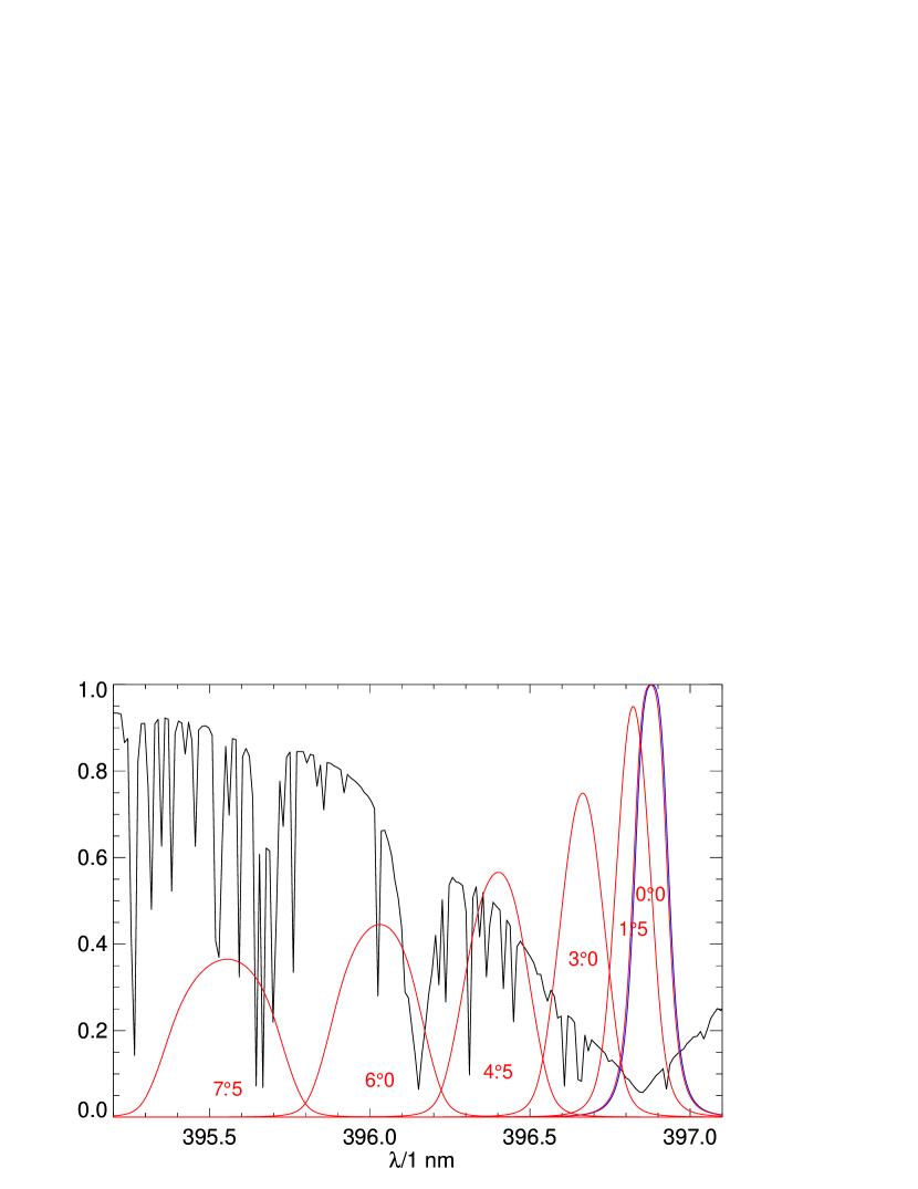
Figure 3: Integrated filter transmittance profiles, $\sum_{x_{p},y_{p}}T_{\text{p}}(\lambda,\theta)$ (red) corresponding to filter tilt angles ($\theta$) as indicated in the figure. The $\theta=0\degr$ profile is virtually identical to the normal incidence filter profile, $T_{\text{f}}(\lambda)$ (blue). The black line is the Ca ii H spectrum of the synthetic data of Sect. 4.

In order to test the predicted broadening and wavelength shifts, the filter was examined using the TRI-Port Polarimetric Echelle-Littrow spectrograph (Kiselman et al. in prep.) at the SST on 2008-05-13. The filter on its rotatable mount was placed in front of the spectrograph slit and the telescope was pointed to solar disk center. Spectra (2000 wavelength points in the range $396.1\text{\leavevmode\nobreak\ nm}\leq\lambda\leq 397.1\text{\leavevmode\nobreak\ nm}$) were collected without the filter, as well as with the filter at 18 different tilt angles that turned out to be $-2\aas@@fstack{\circ}16\leq\theta\leq 5\aas@@fstack{\circ}84$, i.e., angles on both sides of the symmetry point are well represented. The spectra were reduced with standard methods. Filter profiles were then calculated by normalizing the filtered spectra with the unfiltered spectrum. The resulting profiles contain small residues from blending spectral lines which have not been completely removed by the normalization. This is due to the presence of straylight within the spectrograph, which is corrected for in the reductions but the procedure obviously does not work perfectly for spectra of this kind. We deem the resulting profiles good enough for our current purpose, however.

The wavelength scale was calibrated with the help of a spectral atlas (Brault & Neckel 1987) and transformed to the laboratory rest frame. The zero angle is then given by symmetry and the peak wavelength for normal incidence, $\lambda_{\text{c}}=396.89$ nm, follows.

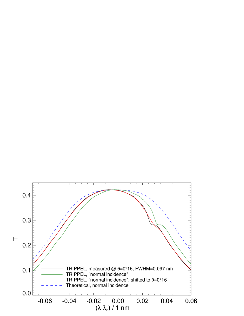
Figure 4: The filter normal incidence transmittance as measured with TRIPPEL. Green: the measured profile shifted towards the red to compensate for tilt angle, our measured $T_{\text{f}}$. Red: model of black curve using measured $T_{\text{f}}$. Black: measured profile with smallest angle. Blue dashed: theoretical $T_{\text{f}}$ (peak reduced to 42%).

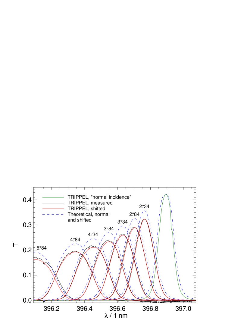
Figure 5: TRIPPEL transmittance measurements at $\theta>2\degr$. Black: measured profiles. Red: models of measured curves using the TRIPPEL-measured “normal incidence” profile. Blue dashed: models of measured curves using the theoretical normal incidence profile with peak reduced to 42%.

In Fig. 4, we show the transmittance profile measured with the smallest angle, 0$\aas@@fstack{\circ}$16. For such small angles, while tilting shifts the central wavelength, it does not broaden the profile significantly. Therefore this should be a good measure of the normal incidence profile $T_{\text{f}}$. We demonstrate that this is so by relocating the measured profile to the symmetry point. Using this to model the measured curve with the filter tilt and pupil apodisation formalism, it is clear that this is just the amount needed for the tilt to shift it back to the measured position and that the match in profile shape is excellent. The only thing that happens to the profile shape is that the small artifact in the red flank is smoothed out slightly. The FWHM of the measured $T_{\text{f}}$ is 0.097 nm rather than the 0.11 nm value from the manufacturer, a significant difference of more than 10%.

The consequences for large angles are shown in Fig. 5. Using the TRIPPEL-measured normal-incidence profile, we can model the measurements very well, which means the profile shift and broadening based on single-cavity theory work well and that the effective refractive index, $n=1.596$, must be a good approximation. Shifting the manufacturer’s profile produces profiles that broaden in the right way, but where the peak transmittance does not decrease with tilt angle fast enough. This is caused by the wider normal incidence profile and the fact that the broadening preserves the area under the profiles.

If a manufacturer is not able or willing to provide an effective refractive index, it should be possible to infer a useful estimate from data like these, by fitting Eq. (8) to the peaks of the shifted profiles.

3.3 Point spread functions and Strehl ratios

The pupil phase for any particular $\theta$ varies with $\lambda$, so it is not obvious what phase, if any, would be effective as a correction of the summed $S_{\text{tilt}}$. In this section we investigate this. We use the theoretical $\tau_{\text{f}}$ profile here, because we have modulus and phase that go together.

The computed MTFs shown in Fig. 6 demonstrate that the tilt is a one-dimensional effect; there is no effect at all in the $y$ direction, perpendicular to the tilt.

The PSFs corresponding to large angles shift significantly in the $x$ direction, as can be seen in Fig. 7. This indicates that there is a significant common tilt in the $x$ direction in the monochromatic wavefronts. This can be understood by noting that in Fig. 2, the monochromatic phases have gradients in the same positions that there are peaks in the modulus. Ignoring the phases produces PSFs that are not shifted and also do not contain the asymmetry in shape that is also evident in the figure.

In real data, we see much larger shifts than the few pixels visible in Fig. 7. In fact, most of the shift is caused by refraction through the glass substrate. An order of magnitude estimate of this shift can be calculated by use of the formula $d=t\theta(n-1)/n$ given by Smith (1990, Chapter 4). With $n=1.596$, thickness $t\approx 5$ mm, and tilt angle $\theta=6\aas@@fstack{\circ}0=0.10$ rad, we get a shift of $d\approx 0.20\leavevmode\nobreak\ \text{mm}=26$ pixels of size 7.4 $\muup$m.

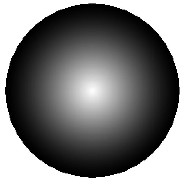
(a) 0$\aas@@fstack{\circ}$0

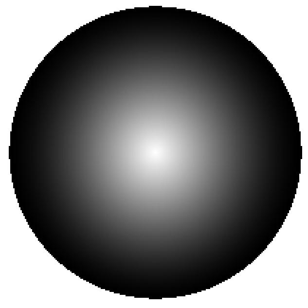
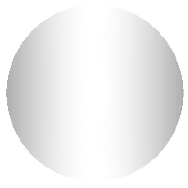
(b) 1$\aas@@fstack{\circ}$5

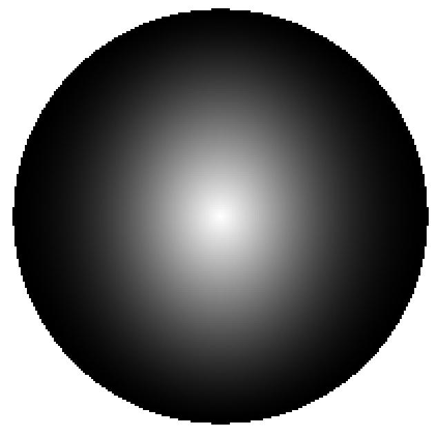
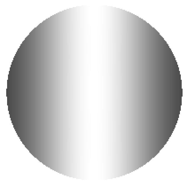
(c) 3$\aas@@fstack{\circ}$0

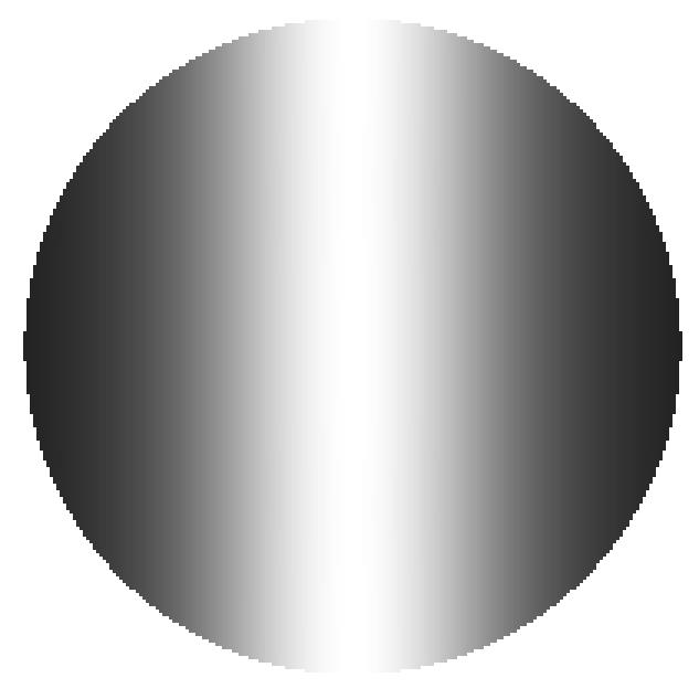
(d) 4$\aas@@fstack{\circ}$5

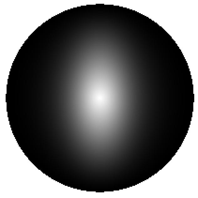
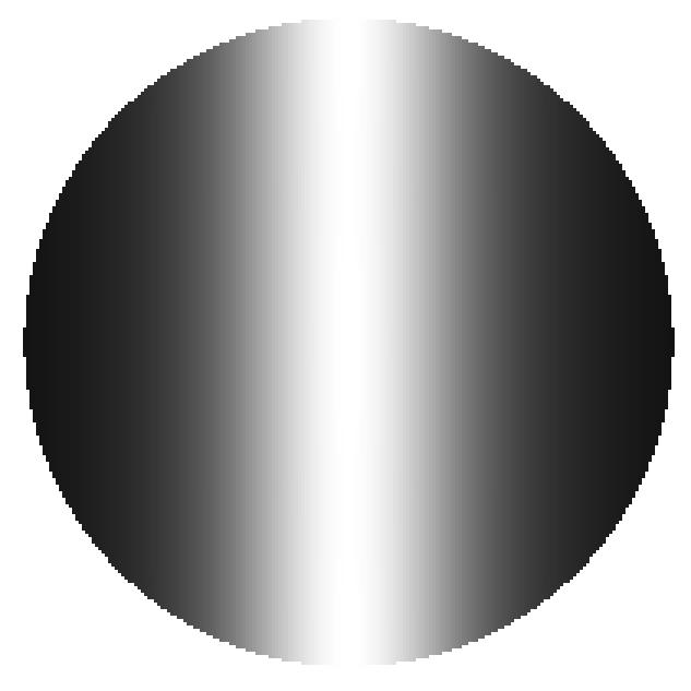
(e) 6$\aas@@fstack{\circ}$0

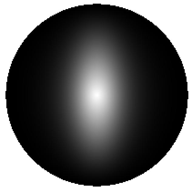
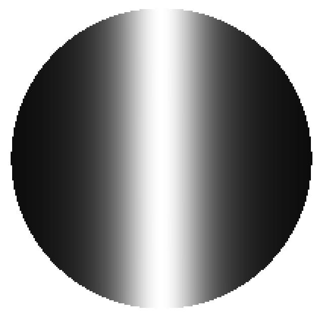
(f) 7$\aas@@fstack{\circ}$5

Figure 6: Top: Diffraction limited MTFs modified by the filter tilt effects, $S_{0}\cdot|S_{\text{tilt}}(\theta)|$; Bottom: Tilt MTFs, $|S_{\text{tilt}}(\theta)|$. Tilt angles $\theta$ as indicated.

(a) 0$\aas@@fstack{\circ}$0

(b) 1$\aas@@fstack{\circ}$5

(c) 3$\aas@@fstack{\circ}$0

(d) 4$\aas@@fstack{\circ}$5

(e) 6$\aas@@fstack{\circ}$0

(f) 7$\aas@@fstack{\circ}$5

Figure 7: Top: PSFs corresponding to $S_{0}\cdot S_{\text{tilt}}(\theta)$; Bottom: PSFs calculated with $\arg\{\tau_{\text{p}}\}$ set to zero. Tilt angles $\theta$ as indicated.

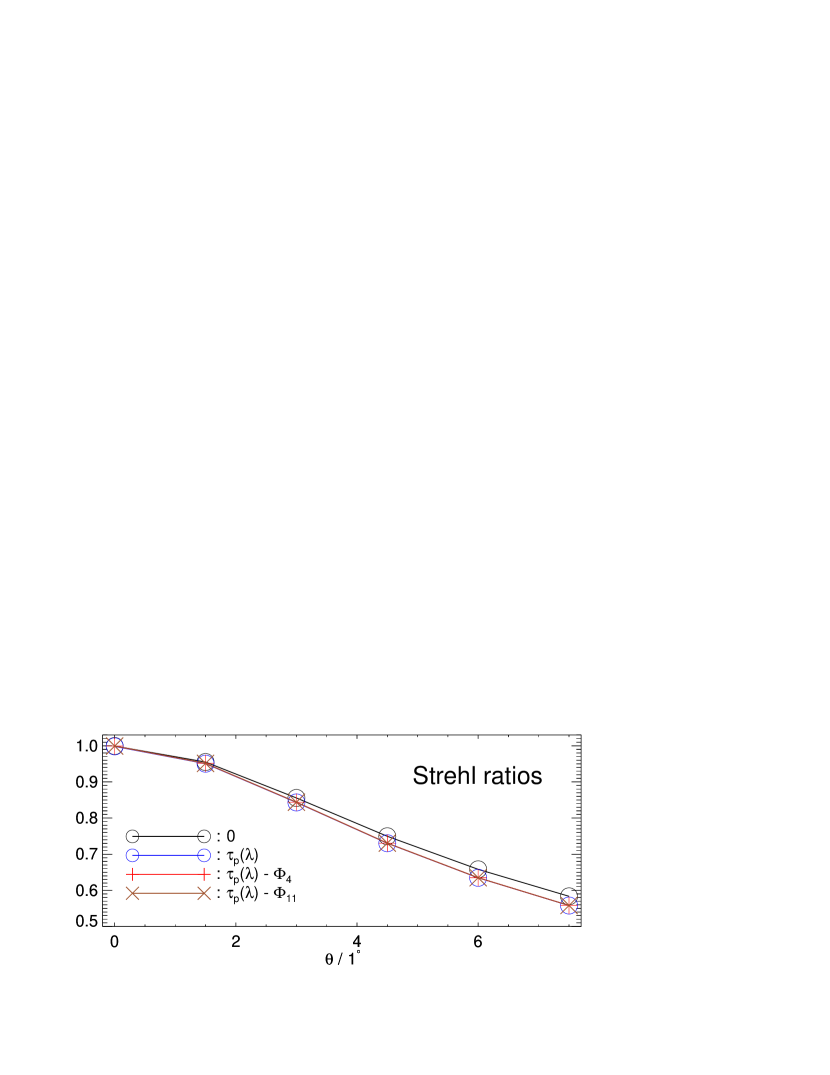
Figure 8: Theoretical Strehl ratios for the Ca ii H filter, calculated by integrating the MTFs. The pupil functions at each wavelength are calculated without the phase, with the phase, and with two different compensations for the phase. $\Phi_{4}$ is an optimum focus term, while $\Phi_{11}$ is an optimized sum of focus, astigmatism, coma, trifoil, and spherical aberrations.

Scharmer (2006) found an optimum focus compensation for the phase effect of a non-tilted FPI by maximizing the Strehl ratio. In Fig. 8, we show Strehl ratios calculated with and without taking the phase of the transmission into account. The Strehl ratio without phase is reduced from almost unity for $\theta=0$ to $\sim$0.6 for 7$\aas@@fstack{\circ}$5. Including the phase reduces the Strehl further, particularly for larger $\theta$. Maximizing the Strehl ratio by varying a common focus compensation we find negligible improvements in Strehl ratio. A tenth of a percent for the small angles, even less for the larger angles. The wavefront RMS of the estimated focus terms ranges from 0.010 waves for $\theta=0\aas@@fstack{\circ}0$ to 0.006 waves for $\theta=7\aas@@fstack{\circ}5$.

The individual apodisations and phases for the non-zero angles are not circularly symmetrical so astigmatism and coma would not be unexpected. However, including Zernike polynomials 4–11 in the optimization gives insignificant additional Strehl improvements and no change in the estimated wavefront RMS. Changes, if any, are in the sixth digit. There is no reason to expect higher order modes to have a significant effect.

The compensated Strehl ratios are also plotted in Fig. 8, where $\Phi_{M}=\sum_{m=4}^{M}c_{m}Z_{m}$ are the optimized phases. $Z_{m}$ are Zernike polynomials, $m=4$ corresponds to focus. It is apparent that the compensations do not alter the Strehl ratios significantly.

This suggests that, at least for this particular setup, the effect of the varying incident angles on the filter should interfere very little with our normal Multi-Object Multi-Frame Blind Deconvolution (MOMFBD; van Noort et al. 2005) restoration practice. Image shifts are already routinely taken care of in calibration of camera alignment by use of a pinhole array. The focus term is compensated already when the camera is focused, usually for $\theta=0\aas@@fstack{\circ}0$. This leaves an uncompensated focus of only 0.004 waves or less at the larger angles, which is insignificant compared to the accuracy of our camera focusing. Evident from the way the PSF moves with angle when the phase is included is that there is also a global tilt term that varies with $\theta$, but this does not change the shape of the PSF.

This means the OTF is to a good approximation separable into an atmospheric wavefront part and a correction for the filter tilt as in Eqs. (16)–(18). The smearing caused by the elongated PSFs affects the SNR by lowering the MTF but should otherwise pass through the MOMFBD processing without changing the estimated phases. The restored object is a version of the real object that is convolved with the PSF corresponding to the apodisation effects without the wavefront phase. This can be taken care of with a simple post-restoration deconvolution step. The consequences for alignment are discussed in Sect. 5.3 below.

4 Synthetic solar data and expected errors

The Strehl experiments correspond to objects that are point-like and do not depend on $\lambda$. However, the solar structures vary with wavelength within the passband of the filter, particularly if it’s broadened and particularly where the line gradient is large. In this section we simulate the formation of solar images by summing the contributions from many wavelengths in a synthetic data cube. We make “perfect” images as well as images based on convolution with either $S_{0}$ or $S_{\text{mono}}$ before summing. We evaluate how well the “perfect” data can be recreated by deconvolving the summed images.

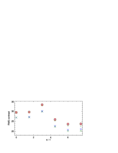
(a)

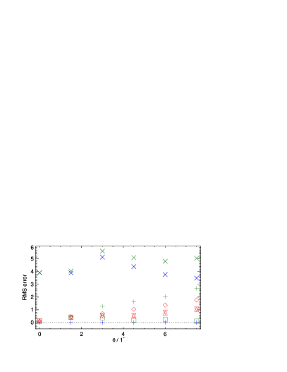
(b)

Figure 9: RMS contrasts (a) and RMS errors (b) from synthetic image deconvolution experiment, both in percent of the mean intensity. Black circles ($\medcirc$, in a only): Synthetic “true” images. Blue symbols: monochromatic images convolved with $S_{0}$ and then summed. The crosses ($\times$) correspond to those images and the pluses ($+$) to the same images after deconvolution with $S_{0}$. Green symbols: monochromatic images convolved with $S_{\text{mono}}(\lambda,\theta)$. The crosses ($\times$) correspond to those images and the pluses ($+$) to the same images after deconvolution with $S_{0}$. The squares ($\square$) correspond to those summed images again, but now deconvolved with $S_{0}\cdot S_{\text{tilt}}(\theta)$. Red symbols: convolved images like for the green symbols but with three types of imperfections in the deconvolution. Up triangles ($\bigtriangleup$): transmission phase not used for calculating $S_{\text{tilt}}$. Down triangles ($\bigtriangledown$): deconvolve with the MTF, $S_{0}\cdot|S_{\text{tilt}}(\theta)|$. Diamonds ($\Diamond$): deconvolution with $S_{0}\cdot S_{\text{tilt}}(\theta)$ mirrored in the $x$ direction.

The synthetic image data cube was calculated from 3D MHD simulations kindly provided by Mats Carlsson and based on the code by Stein & Nordlund (1998). We used MULTI (Carlsson 1986), a Ca ii H 5-level atom model, and line opacities from the Vienna Atomic Line Database (Piskunov et al. 1995; Kupka et al. 1999, 2000) for the line blends. The data cube comprises a wavelength range covering the tunable filter range ($394.2\text{ nm}\leq\lambda\leq 399.5\text{ nm}$, $\delta\lambda=0.01\text{ nm}$). The most relevant part of the spectrum is shown in Fig. 3.

Because we have established separability in Sect. 3.3, we do not have to include atmospheric turbulence in these simulations. The experiment corresponds to images that are perfectly restored from those effects by image restoration with methods such as MOMFBD or Speckle interferometry. We included neither noise nor stray light in these simulations.

The results of the experiments can be found in Fig. 9. The RMS errors are calculated as the standard deviation of the difference of an image and the “perfect” image, after subpixel alignment. The errors therefore measure only the residual blurring and not errors from image shifts caused by off-center and asymmetrical PSFs.

The circles in Fig. 9a represent the RMS contrasts of the “true” images. These contrasts vary between 23.5% and 33.3% because of the varying heights in the solar atmosphere where they are formed. Convolving each monochromatic image in the synthetic data cube with the diffraction-limited PSF before summing, i.e., multiplying the Fourier transform with $S_{0}$, makes the contrasts drop as shown with the blue crosses, resulting in RMS errors in the range 4–5% as shown in Fig. 9b. Deconvolving with $S_{0}$ recreates the original contrasts and brings the errors down to zero as expected (blue pluses).

For the remaining experiments, $S_{\text{mono}}$ was applied to each monochromatic image before summing. The contrast drops a bit more than for $S_{0}$, particularly for the larger tilt angles $\theta$ and the RMS errors are larger (green crosses). Consequently, deconvolving with $S_{0}$ works well for the small angles but not for the larger angles (green pluses). In fact, for 0$\aas@@fstack{\circ}$0 and 1$\aas@@fstack{\circ}$5, it does not matter much whether we deconvolve with $S_{0}$, $S_{\text{tilt}}$ or any of the imperfect OTFs described in the next paragraph.

For the larger angles, deconvolving with $S_{0}\cdot S_{\text{tilt}}$ also restores the original contrasts and reduces the errors to small fractions of the $S_{\text{mono}}$ versions. However, when using imperfect versions of $S_{\text{tilt}}$ (red symbols) the results for the larger angles is worse. Not using the phase of the transmittance profile, $\arg(\tau_{\text{f}})$, gives approximately the same RMS errors as correcting only for the MTF, $S_{0}\cdot|S_{\text{tilt}}|$, which is expected since neither can represent the asymmetry of the PSFs (red upward and downward triangles, resp.). Even worse is to use the asymmetric PSFs, but reversed (red diamonds).

5 Real data and consequences for image restoration

In this section, we work with SST data collected by Henriques et al. (in prep.) in May 2010. We used four MegaPlus II es4020 cameras with 2048$\times$2048 7.4-$\muup$m pixels. The beam was F/46 and the image scale is 0$\aas@@fstack{\prime\prime}$034/pixel. There was 23% oversampling in the Fourier domain.

One camera collected data throught the tilt-mounted NB filter. The observing programme specified tilt angles $\theta=1\aas@@fstack{\circ}2$, 2$\aas@@fstack{\circ}$5, 3$\aas@@fstack{\circ}$0, 3$\aas@@fstack{\circ}$7, 4$\aas@@fstack{\circ}$2, 4$\aas@@fstack{\circ}$8, and 6$\aas@@fstack{\circ}$4. These angles correspond to passbands with the central wavelengths $\lambda_{\text{c}}=396.84$, 396.74, 396.67, 396.57, 396.47, 396.34, and 395.93 nm, respectively, chosen to sample interesting heights in the solar atmosphere. In addition, we had two cameras behind a wideband (WB) filter centered on 395.37 nm (FWHM 1.0 nm), one in the conventional focus and one defocused by 7 mm for approximately 1 wave peak-to-peak of focus PD. The fourth camera was mounted behind a fixed NB (FWHM 0.1 nm) 396.47 nm wing filter.

We routinely perform a calibration step, where we collect data while scanning the filter through a large range of angles, approximately centered on $\theta=0\degr$ (in the case of these data: 20° with 0$\aas@@fstack{\circ}$1 resolution). We calculate the average intensities of the images and find the zero position by looking for the symmetry point. Because these data depend on the unknown spectrum, we do not model these data in order to draw any conclusions besides the zero tilt angle.

5.1 Pinhole images and OTF correction

As part of the standard calibration procedures at the SST, we collect data through artificial targets mounted in the primary (Schupmann) focus. One such target, designed for measuring straylight, consists of six holes of diameters that range from 20 $\muup$m to 1 mm. We can use these to test our calculated $S_{\text{tilt}}$ corrections. We use a 512$\times$512-pixel subfield with only the smallest, barely resolved pinhole.

In order to gain SNR, we co-added many frames (each with an exposure time of 10 ms), aligned to subpixel precision. The available number of frames from this campaign is 500 in each of the tilted NB wavelengths and 3500 in the WB. The individual frames are dark corrected by subtraction of an average dark frame. After co-adding, an extra dark correction step is performed. All summed images were normalized to the average intensity within the 1-mm hole. A refinement dark level for the WB image was calculated as the median of the outer few rows and columns of the 512$\times$512-pixel subfield and subtracted from the WB image. The NB images were then dark corrected by subtraction of the amount needed to make the total intensity the same in all images.

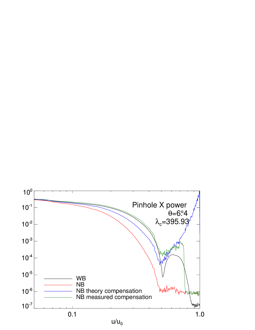
Figure 10: Straylight target pinhole power spectra in the $x$ direction, affected by the 6$\aas@@fstack{\circ}$4 tilt. Angular averages within $\pm 22.5\degr{}$ wide sectors centered on the axis directions. Calculated using a 1024$\times$1024-pixel subfield of the detector FOV. NB: original, corrected with theoretical MTF, and corrected with measured MTF (or OTF, the corrected powers are the same). WB for comparison (covered by the NB compensated line). The TRIPPEL measured profile was used for the theoretical correction. Using the theoretical profile gives even less correction.

The power of the pinhole image is isotropic in the WB but not in the NB because of the tilt effect. In the $y$ direction the WB and NB powers are equal but in the $x$ direction, the NB power is attenuated. We demonstrate this for $\theta=6\aas@@fstack{\circ}4$ in Fig. 10, compare the black and red curves. Note the dip in power at approximately 50% of the diffraction limit. There is a corresponding dip in the NB power, although not as clearly visible because the power spectrum is so noisy at the spatial frequencies beyond the dip. These dips are caused by a zero-crossing in the Fourier transform of the target. The Fourier transform of a pillbox function (representing a circular pinhole) is a radial jinc function. Such zero crossings appear closer to the origin the larger the hole is, so the smaller the hole, the better. In the limit of zero diameter we have a $\delta$ function, the transform of which is a constant.

Correcting the NB power by use of the theoretical $S_{\text{tilt}}$ is not enough, as evidenced by the blue curve. We show here the theoretical correction based on the profile measured with TRIPPEL. Using the manufacturer’s theoretical profile results in even slightly less correction.

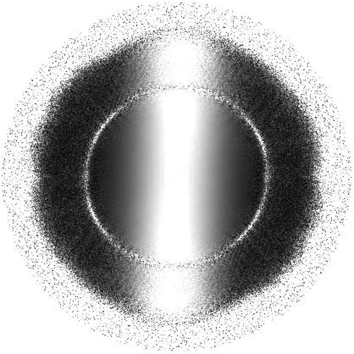
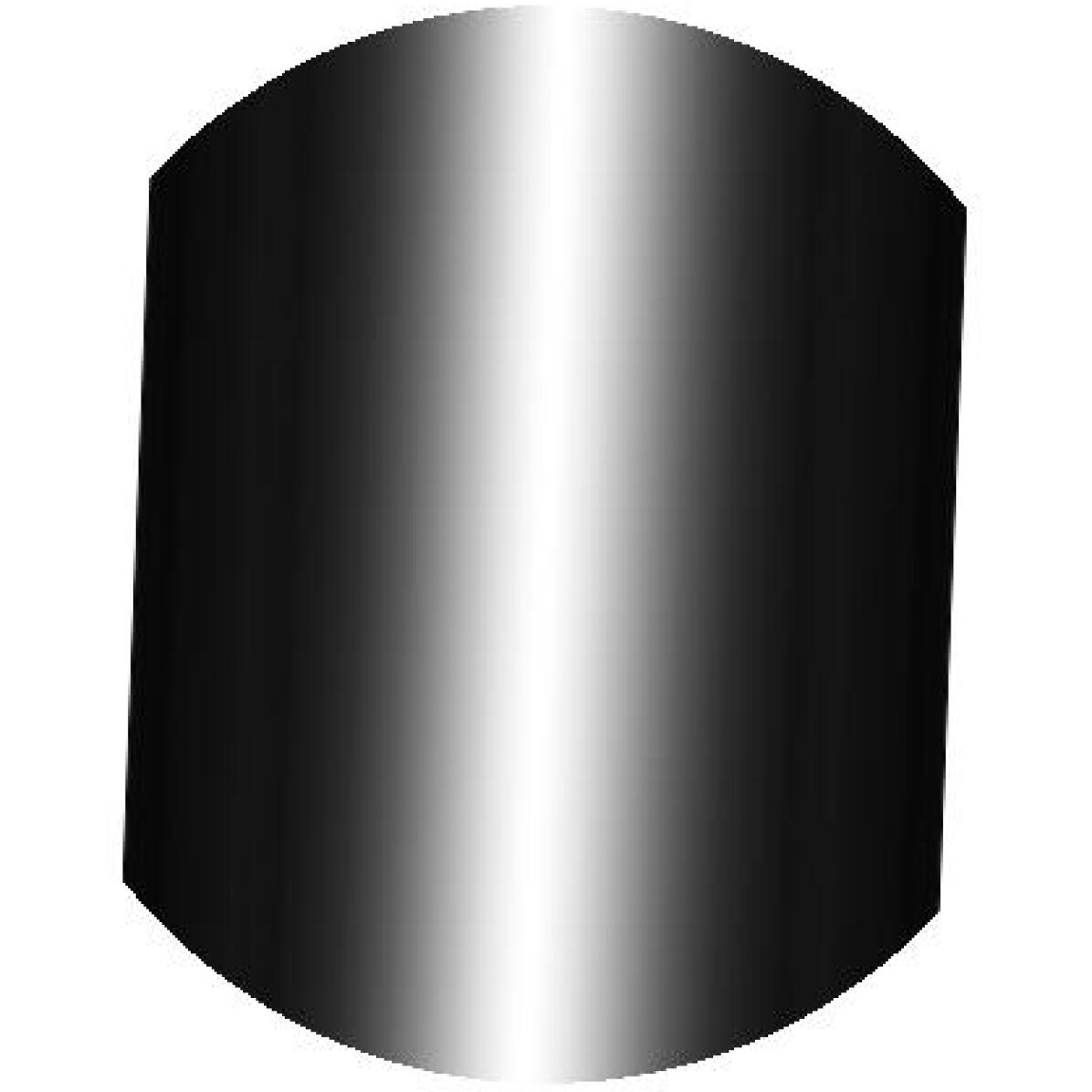
(a) 6$\aas@@fstack{\circ}$4

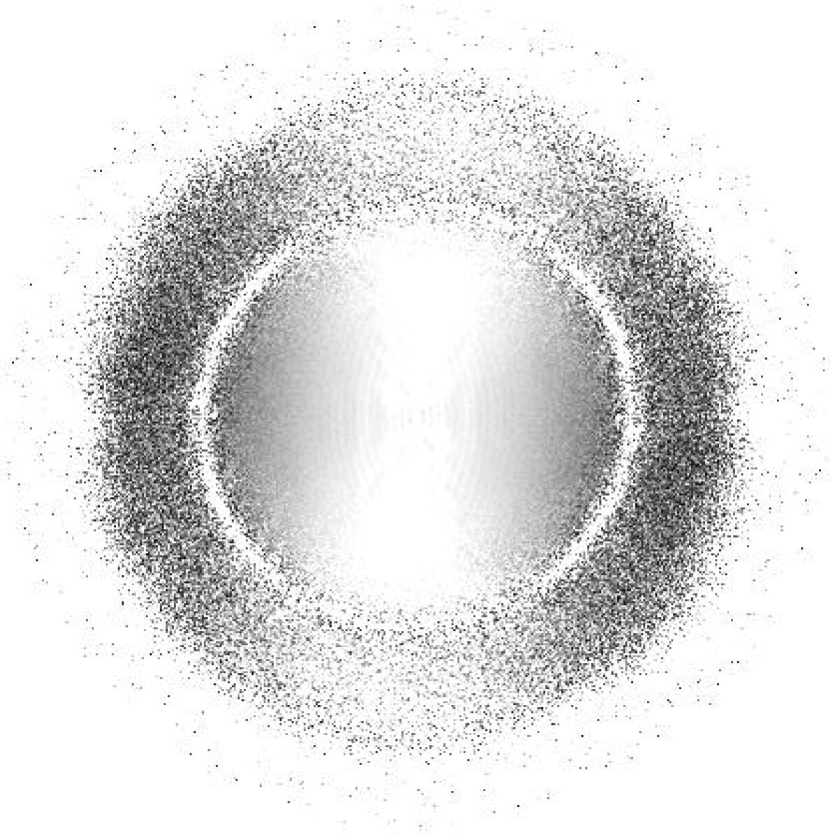
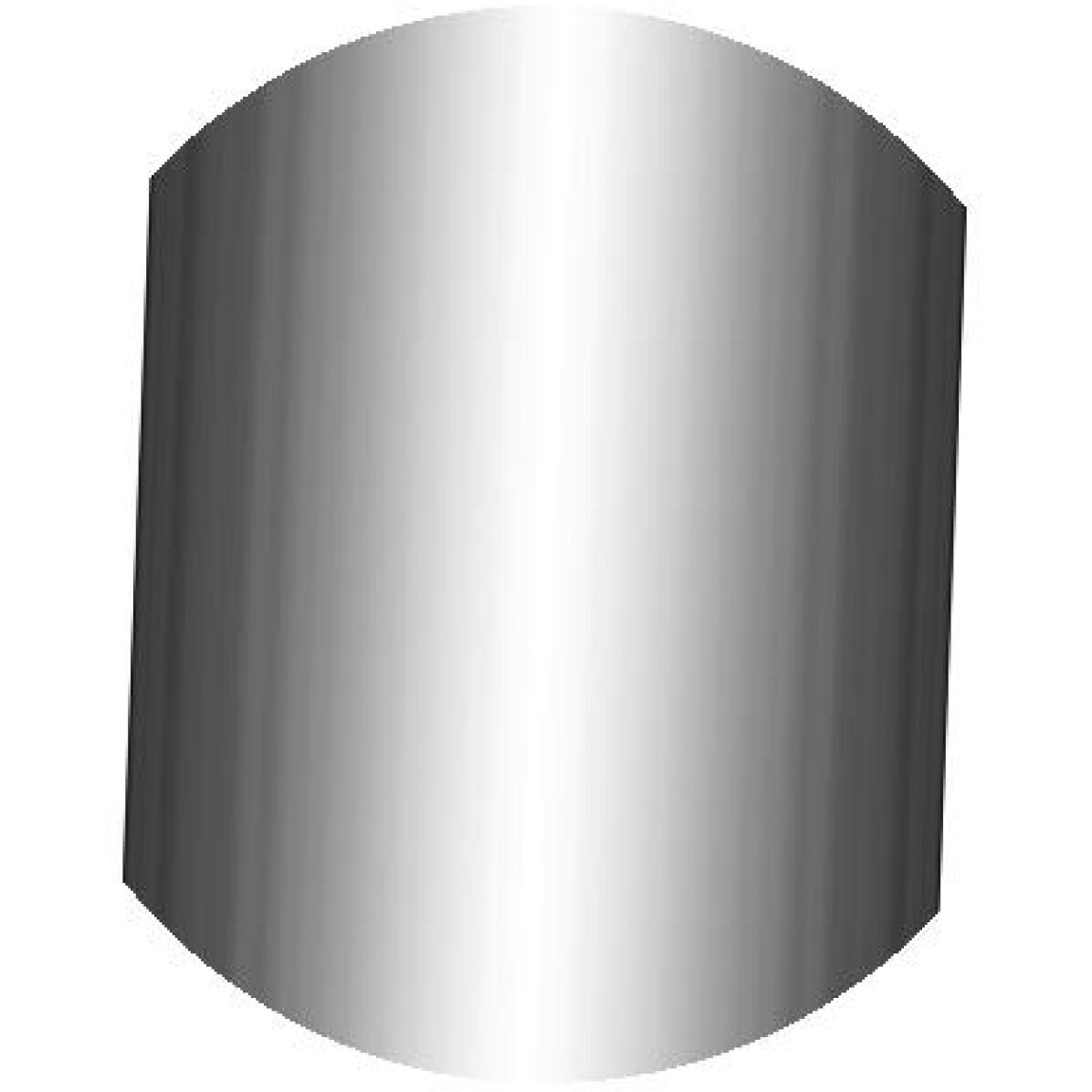
(b) 3$\aas@@fstack{\circ}$0

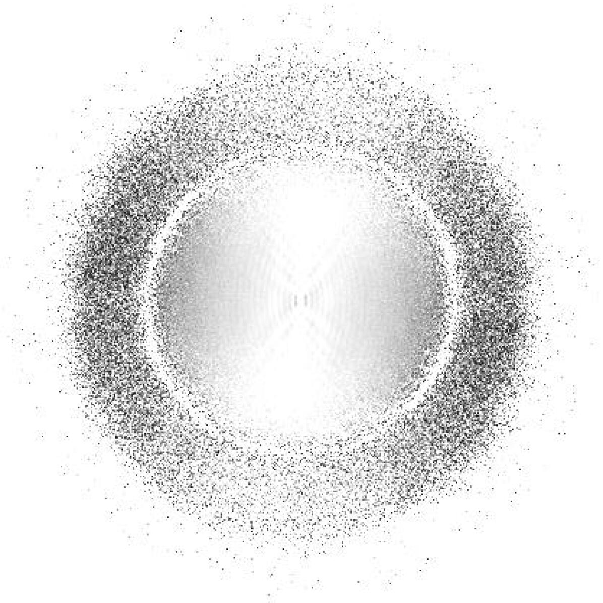
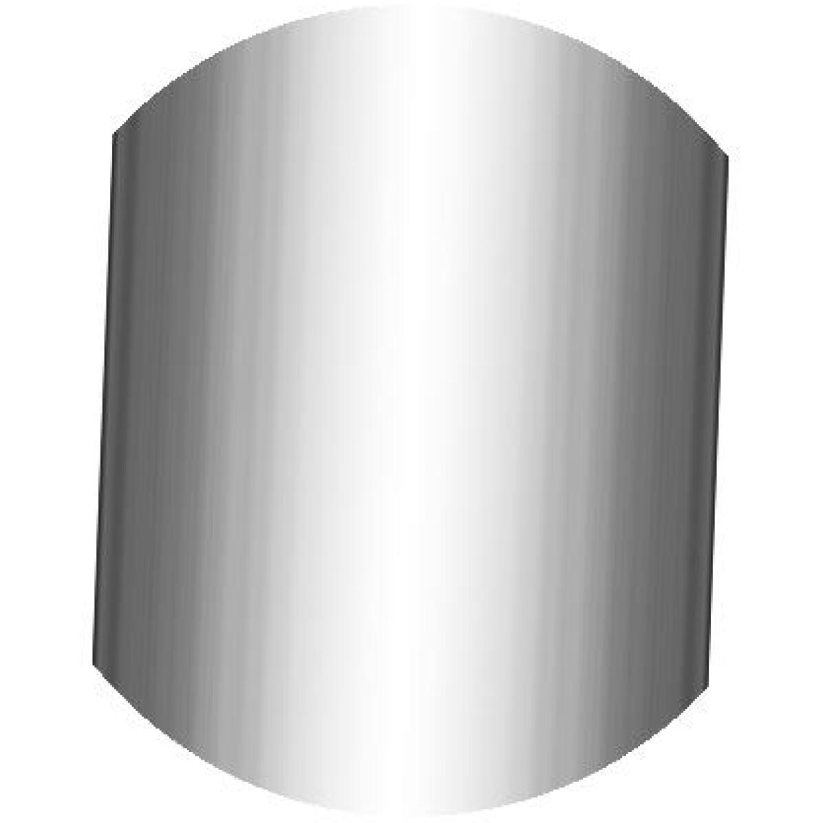
(c) 2$\aas@@fstack{\circ}$5

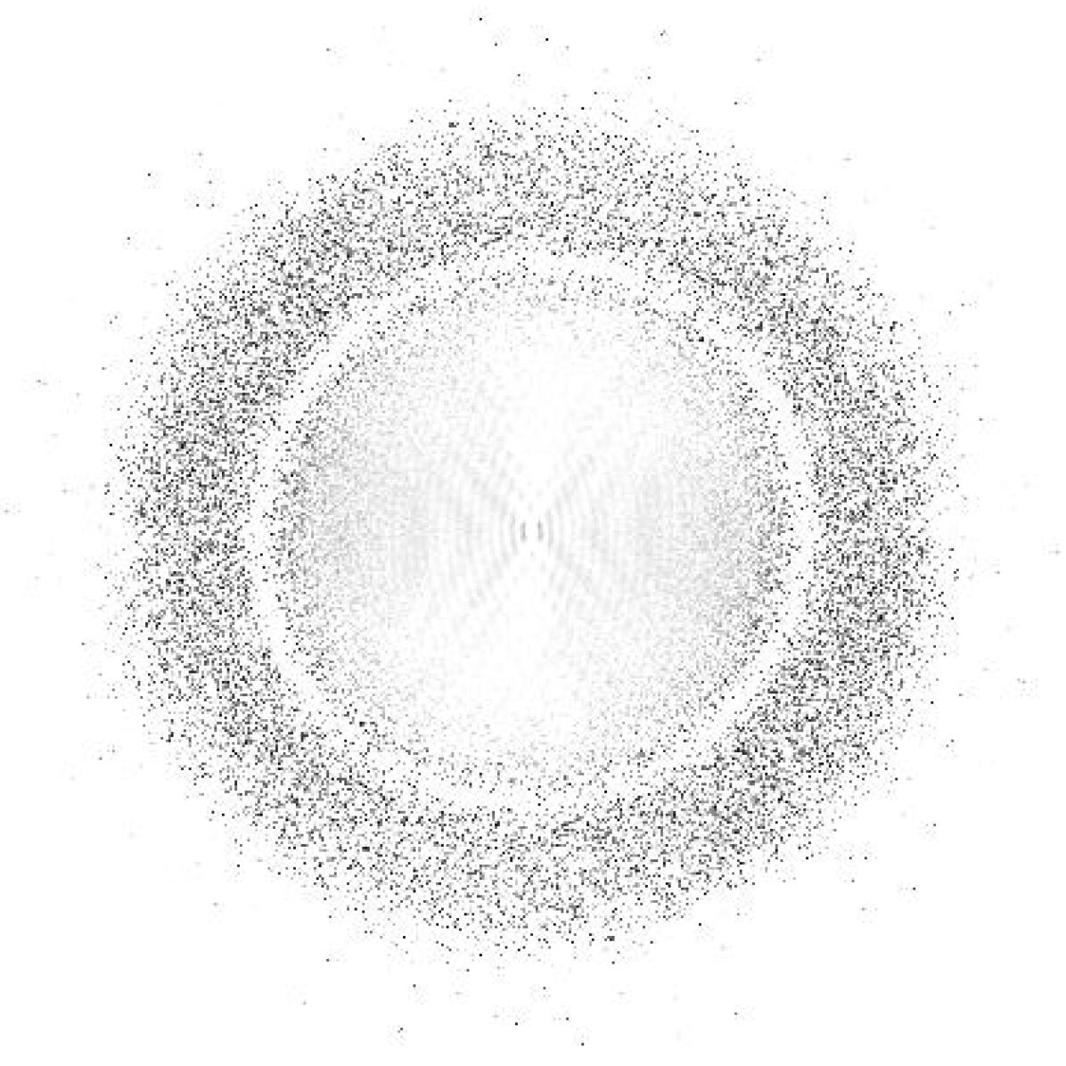
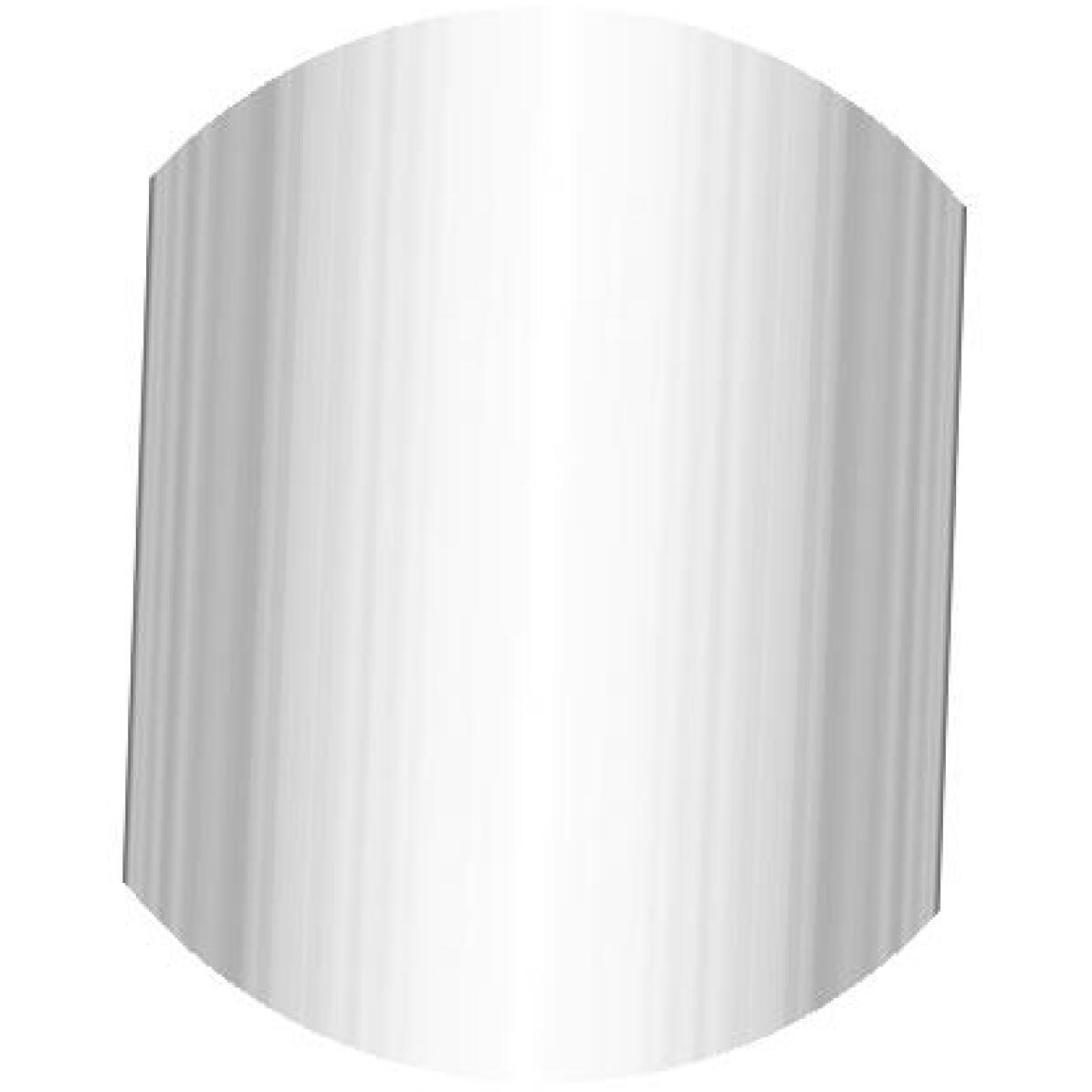
(d) 1$\aas@@fstack{\circ}$2

Figure 11: Measured MTF correction $|S_{\text{tilt}}(\theta)|$ based on straylight target pinhole power. Top: Dirty; Bottom: Cleaned. Tilt angles $\theta$ as indicated. The circumferences represent the diffraction limit. The orientation of the ridge is $\sim$2° from the $y$ axis. Compare with Fig. 6.

However, because the pinhole is the same in WB and NB, it should be possible to measure $S_{\text{tilt}}$. We can get a first estimate by taking the ratio of the Fourier transforms of the two images,

$$\frac{D_{\text{NB}}}{D_{\text{WB}}}=\frac{FS_{\text{wf}}S_{\text{tilt}}}{FS_{\text{wf}}}=S_{\text{tilt}},$$ (20)

where $S_{\text{wf}}$ is here the OTF representing phase aberrations in the optics on the optical table. The results for a few tilt angles are shown in the top row of Fig. 11. These “dirty” measurements are dominated by noise at the higher spatial frequencies. However, since we know from Fig. 6 that they should be constant in the $y$ direction, it should be possible to clean them.

The ring at about 50% of the diffraction limit corresponds to the jinc dip in WB power. We mask this ring-shaped zero crossing artifact and calculate the median along the direction that is supposed to be constant. We smooth the result and then construct a cleaned 2D $S_{\text{tilt}}$. In the real data, this direction is not exactly parallel to the $y$ direction, so we first find the orientation of the ridge, rotate $S_{\text{tilt}}$, do the cleaning and rotate the result back to the original orientation. The result is in the bottom row of Fig. 11.

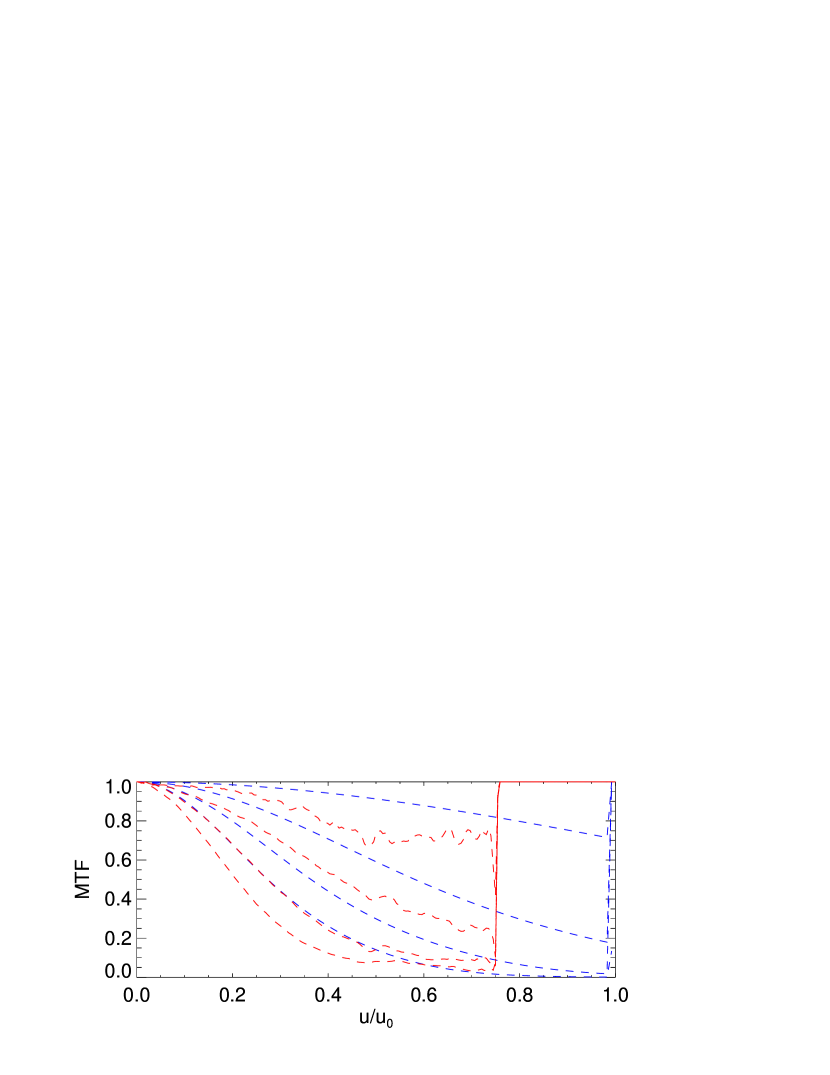
Figure 12: MTF corrections, $|S_{\text{tilt}}(\theta)|$, in the $x$ direction for $\theta=1\aas@@fstack{\circ}2,3\aas@@fstack{\circ}0,4\aas@@fstack{\circ}8,6\aas@@fstack{\circ}4$ (from top to bottom). Blue: theoretical MTFs; Red: measured MTFs.

We show the theoretical and measured corrections for a few angles in Fig. 12. Note the discrepancies between the blue curves and the corresponding red curves! For the present data, the limit to where we can measure $S_{\text{tilt}}$ in the $x$ direction is set by the SNR in the WB pinhole image in the denominator to a little less than 80% of the diffraction limit. We define $S_{\text{tilt}}$ to be unity outside this limit. Noise in the NB (numerator) is worse for the smaller angles because the Sun is darker in the core of the spectral line, the irregularities caused by this are apparent in the figure.

It is apparent that we need more exposures to construct $S_{\text{tilt}}$ functions that go all the way to the diffraction limit in the $x$ direction, and that are not noise dominated above 50% of the diffraction limit. The noisy NB bump in Fig. 10 suggests that we need to increase the number of NB frames by an order of magnitude or more. With an image rate of 10 frames/s, it should be possible to collect $\sim$5000 images in 8 min. With seven tilt angles, this corresponds to almost an hour. However, this kind of data would not have to be collected each day or even by each observer interested in this kind of correction.

5.2 Solar images

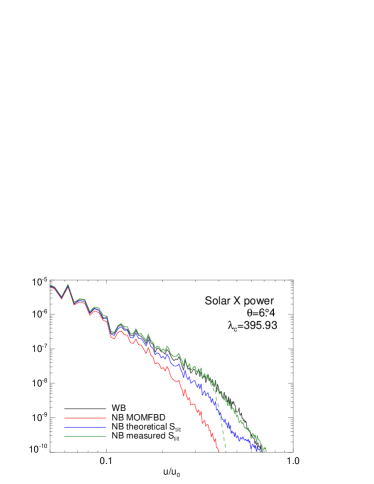
(a)

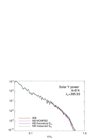
(b)

Figure 13: Solar power spectra, angular averages within $\pm 22.5\degr{}$ wide sectors centered on the axis directions. LABEL:sub@fig:solpowx In the $x$ direction, where the tilt effects are; LABEL:sub@fig:solpowy In the $y$ direction, unaffected by the tilt effects. The dashed line represents noise filtered data.

On 2010-05-23, we collected solar images with an exposure time of 10 ms near disc center ($\mu\approx\cos 20\degr\approx 0.94$). Together with the WB, WB PD, and fixed NB data, the tilt-tuned NB images were restored for atmospheric turbulence effects with MOMFBD using the 36 most significant atmospheric Karhunen–Loève modes. Observations and MOMFBD processing will be described in detail by Henriques et al. (in prep.).

Figure 13 shows power spectra for $\theta=6\aas@@fstack{\circ}4$. For this angle, the central wavelength of the NB passband has shifted to 395.93 nm, well within the passband of the WB filter. Here, the granulation has the same power in the $y$ direction in NB as in WB, see Fig. 13b. We can expect this to be the case also in the $x$ direction, which can be used for testing our $S_{\text{tilt}}$ compensation. In Fig. 13a, the MOMFBD restored NB power (red) is attenuated compared to the WB power (black). Just as for the pinholes, the theoretical $S_{\text{tilt}}$ compensation (blue) does not fully correct the asymmetry in power, but the measured compensation does (green).

(a)

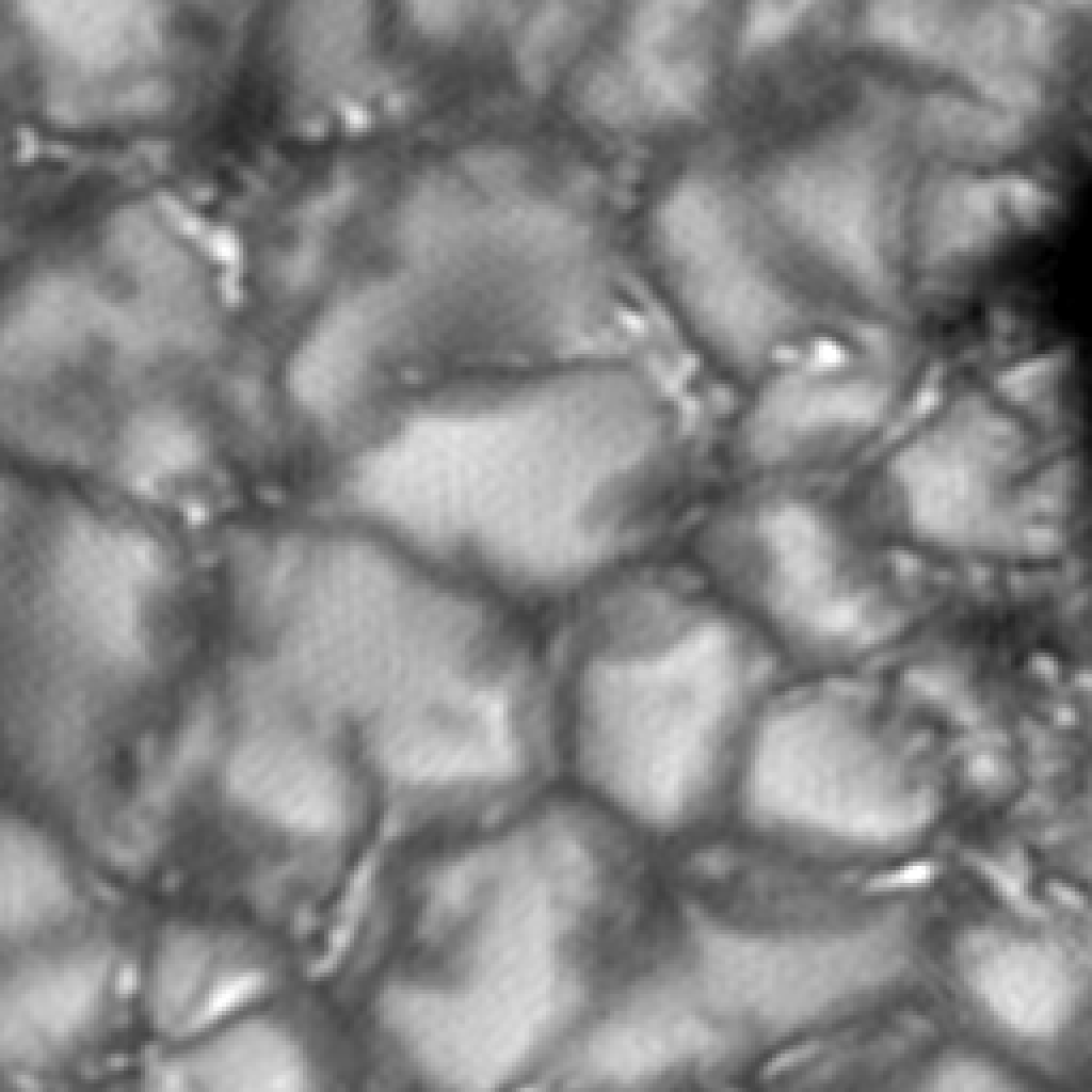
(b)

(c)

Figure 14: An 11″$\times$11″ solar image collected with 6$\aas@@fstack{\circ}$4 filter tilt. (a) Restored with MOMFBD; (b) Compensated for tilt effects by use of the measured $S_{\text{tilt}}$; (c) Compensated and noise filtered.

There are visible effects in the images, that correspond to the correction of the anisotropy in the power spectrum. Compare the MOMFBD restored image in Fig. 14a and the same image after correction for $S_{\text{tilt}}$ in Fig. 14b. Because $S_{\text{tilt}}$ makes point-like objects elongated in the $x$ direction, the effect is most easily seen in the smallest structures. For example, strings of small bright features oriented in the $x$ direction are more clearly separated after $S_{\text{tilt}}$ correction, while such strings oriented in the perpendicular direction mainly get higher contrast with respect to the surrounding dark lanes.

The $S_{\text{tilt}}$ compensation enhances the noise somewhat, particularly for the larger angles, so we need to use a noise filter. Figure 14c shows the compensated image filtered with the noise filter in Fig. 15a. The noise filter is very asymmetrical, as it should because the attenuated power in the $x$ direction will fall to the noise level faster than the $y$ power. The noise filter seems to be correct in that it removes the noise without visibly changing the resolution in the smallest structures. This is also the case for the noise filters constructed for the other tilt angles.

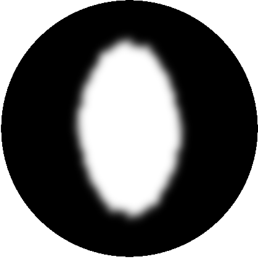
(a) 6$\aas@@fstack{\circ}$4

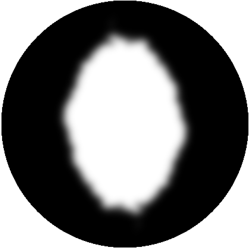
(b) 4$\aas@@fstack{\circ}$8

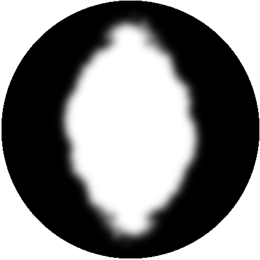
(c) 4$\aas@@fstack{\circ}$2

Figure 15: The low-pass noise filter for the largest angles. The perimeter of the circle represents the diffraction limit.

Table 1: Observed RMS contrasts.

Deconvolution	NB							WB
	1$\aas@@fstack{\circ}$2	2$\aas@@fstack{\circ}$5	3$\aas@@fstack{\circ}$0	3$\aas@@fstack{\circ}$7	4$\aas@@fstack{\circ}$2	4$\aas@@fstack{\circ}$8	6$\aas@@fstack{\circ}$4
$S_{\text{atm}}$	25.7	16.5	15.4	13.1	12.0	12.2	12.9	13.3
$S_{\text{atm}}S_{\text{tilt}}(\theta)$	25.8	16.6	15.6	13.6	12.4	12.7	13.6

For a proper Wiener-type noise filter, one needs the signal power and the noise power. The original, raw-data noise at the highest spatial frequencies is already filtered out by the MOMFBD restoration. Instead, there is a noise that comes from the mosaicking of subfields done as part of the MOMFBD processing. The power of this noise seems to vary with spatial frequency in a way similar to the signal but extend to higher spatial frequencies. The filters in Fig. 15 are based on thresholding the power spectrum of the uncompensated NB image at levels found by trial and error. The filters are then made from the resulting binary images by closing holes and removing isolated pixels, and finally smoothing with a Gaussian kernel.

For images to be used for making differential quantities (like magnetograms or Doppler maps), it is best to use the same low-pass noise filter. Otherwise, there will be spatial frequencies with information missing in some images but not in others. A simple way of constructing such a filter is to form, in every Fourier domain pixel, the minimum of the filters for the relevant images. Such a combination of the filters shown in Fig. 15 would be very similar to the 6$\aas@@fstack{\circ}$4 filter.

The contrasts in Table 4 are much lower than those in Fig. 9 because of various sources of stray light, see discussion by Scharmer et al. (2010). The contrasts show the expected increase in contrast with $S_{\text{tilt}}$ compensation, more for large $\theta$ than for small.

5.3 Image shift and MOMFBD processing

A very useful property of the Multi-Object part of MOMFBD image restoration is that the restored images of the different objects are delivered by the program, aligned to subpixel precision (van Noort et al. 2005). In this context, different “objects” refer to the same patch of the Sun, but imaged in different wavelengths and/or different polarization states. This ability facilitates the calculation of physical quantities based on combinations of these objects with a minimum of artifacts from misalignment. When the images are co-spatial and co-temporal, they are subject to the same wavefront aberrations and are therefore blurred and shifted by the same PSFs (or PSFs that differ in easily modeled ways). The alignment is accomplished by a pre-processing step, where local shifts are measured in images of an array of pinholes, which provides enough information for the MOMFBD program to compensate for fixed differences in alignment and, to some extent, in rotation or image scale.

Compensation for $S_{\text{tilt}}$ interferes with this procedure because the corresponding PSF is off-center and therefore shifts the images. If the MOMFBD-restored images are shifted in a post-processing step, it is necessary to make sure the pinhole array images are shifted the same way before the local-shift measurements are done. So the pinhole array images should be $S_{\text{tilt}}$ compensated before the pre-processing step.

However, the difference in shifts for large and small tilt angles can be several pixels, see Fig. 7. Applying the compensation to the pinhole images means the subfield grid used for the corresponding objects will be off by the same number of pixels. This is then corrected for in the post-processing step, where the restored images are $S_{\text{tilt}}$ compensated, but it is likely that the alignment works better if the subfield grids are aligned during the MOMFBD process. This can be accomplished if the $S_{\text{tilt}}$ PSFs are centered before they are used. We believe it is enough and possibly safest to do this to nearest pixel and avoid subpixel operations for this step.

We therefore recommend the following steps, which we have tested with our data set:

1. Calculate $S_{\text{tilt}}(\theta)$ for all $\theta$ and center the corresponding PSFs to nearest pixel precision.

2. Deconvolve the pinhole array images with these centered PSFs.

3. Perform the standard pre-processing step using the deconvolved pinhole array images.

4. Do normal MOMFBD processing.

5. Deconvolve the restored images with the centered PSFs.

6 Conclusions

We have investigated a NB double-cavity filter, used at the SST for scanning through the blue wing of the Ca ii H spectral line.

Measurements with the TRIPPEL spectrograph show that the filter has a passband that is narrower by 10% than indicated by profiles obtained from the manufacturer. We note that the filter was 8 years old at the time of these measurements but we know too little about coating age effects to speculate on why this can happen. These measurements also indicate that a description based on wavelength shifts of single-cavity filter profiles, together with a model for variations in the incident angle over the pupil, work very well for predicting the position and shape of the broadened passband.

We calculate PSFs and OTFs corresponding to a diffraction limited telescope and tilt angles in the range 0$\aas@@fstack{\circ}$0–7$\aas@@fstack{\circ}$5 and find that the Strehl ratio decreases to less than 0.6 for the largest angle.

We find that the tilt effects couple very weakly with wavefront corrections and that the OTFs are separable in the usual OTF for phase aberrations (including atmospheric turbulence effects) and $S_{\text{tilt}}$, a correction for the filter tilt effects. This means it is sufficient to correct images after restoration for atmospheric effects, the raw data do not have to be corrected before image restoration. However, the PSFs are in general off-center and asymmetric, which has consequences for MOMFBD alignment. We have designed a procedure for $S_{\text{tilt}}$ compensation in a way that maintains the alignment properties of MOMFBD image restoration.

By experiments with synthetic data, we find that deconvolution with the proper OTF compensates very well for the degrading effects that are really affecting the image formation at each wavelength in the passband separately. We demonstrate the effect of the phase of the transmission profile and show that not allowing for this phase in the right way can significantly increase the RMS error in the compensated images.

Our theoretical model for pupil apodisation effects from varying incident angles on NB interference filters does not adequately predict the effects on image quality. This is evident from power spectra of pinhole images as well as solar data. This can be an error in our derivations or coding, but we note that it would have to be a mistake that affects $S_{\text{tilt}}$ without causing errors in the profile broadening.

Instead, we find that useful $S_{\text{tilt}}$ can be measured by use of pinhole calibration data. The ones we measure are visibly affected by noise but this can easily be improved by use of data with better SNR. Note that the better the solar data, the better pinhole images are needed.

For the specific setup with a tilt-tunable Ca ii H filter at the SST, the degrading effect on the PSF is negligible when the filter is not tilted, but becomes more significant as the tilt angle is increased.

A filter wheel with fixed passband filters or an FPI are better ways of sampling different positions in a spectral line. However, tuning interference filters by tilting them from normal incidence is useful because it is a cheaper solution. It may be preferable if one can live with the spectral broadening and compensate for the degraded resolution.

Appendix A The incident angle

This appendix gives a derivation of an expression for the incident angle $\alpha$ on a filter in a converging beam as a function of position in the pupil. We use a coordinate system with the unit length equal to the pupil diameter, $D$. The distance between the pupil and focal planes is then equal to the F-ratio, $F=f/D$, where $f$ is the focal length.

A ray emanates from the pupil plane at the point $(x_{\mathrm{p}},y_{\mathrm{p}},0)$ and intersects the detector in the focal plane at $(x_{\mathrm{f}},y_{\mathrm{f}},F)$. The filter can be anywhere between the pupil and the detector and it is tilted by an angle $\theta$ around an axis parallel to the $y$ axis. The geometry of the pupil–filter system is shown in Fig. 16.

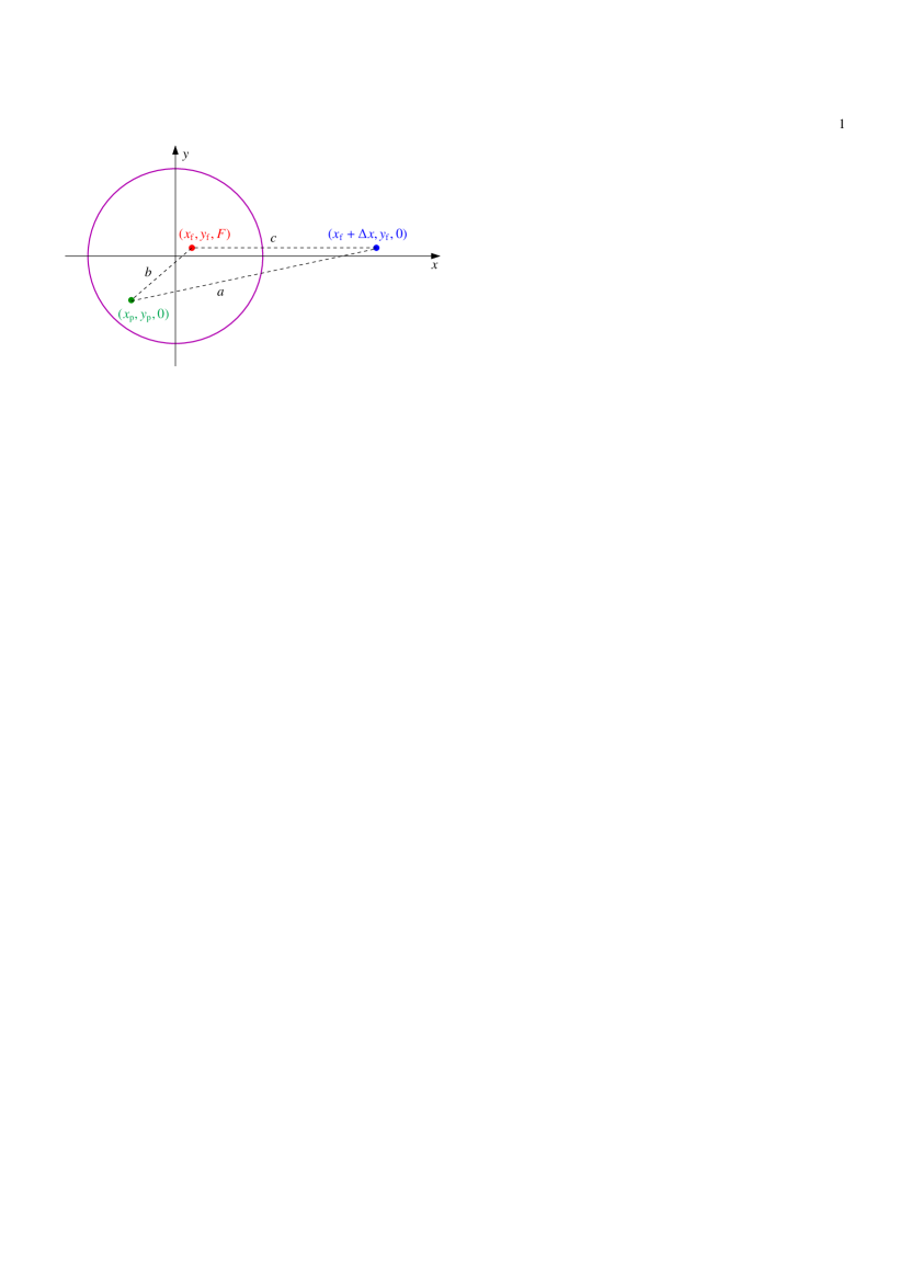
(a) Pupil plane

(b) Horizontal plane

Figure 16: Filter tilt geometry. (a) Projected on the pupil plane. (b) Top view, projection on the horizontal plane. The pupil with diameter $D=1$ is indicated by the circle in a) and by the two tick marks on the $x$ axis in b). The focal length is $f$. In $(x,y,z)$ space ($z$ is the optical axis), a ray leaves the pupil plane at $(x_{\mathrm{p}},y_{\mathrm{p}},0)$ and hits the detector in the focal plane at $(x_{\mathrm{f}},y_{\mathrm{f}},F)$. The filter surface normal from $(x_{\mathrm{f}},y_{\mathrm{f}},F)$ intersects with the pupil plane at an $x$-coordinate increased by an amount $\Delta x$ given by Eq. (25). The angle $\theta$ is in a horizontal plane but $\alpha$ is in general not.

The Law of Cosines gives a relation between the incident angle $\alpha$ and the lengths of the sides in the $abc$ triangle,

$$a^{2}=b^{2}+c^{2}-2bc\cos\alpha,$$ (21)

where $a$, $b$, and $c$ are the distances between the triangle corners,

$$a^{2} =(x_{\mathrm{f}}+\Delta x-x_{\mathrm{p}})^{2}+(y_{\mathrm{f}}-y_{\mathrm{p}})^{2},$$ (22)

$$b^{2} =(x_{\mathrm{p}}-x_{\mathrm{f}})^{2}+(y_{\mathrm{p}}-y_{\mathrm{f}})^{2}+F^{2},$$ (23)

$$c^{2} =\Delta x^{2}+F^{2}.$$ (24)

The length $\Delta x$ is given by the filter tilt angle $\theta$ as

$$\Delta x=F\tan\theta.$$ (25)

For $|\theta|\leq\pi/2$, Eqs. (21)–(25) and trivial algebra yield

$$\cos\alpha=\frac{F\cos\theta+(x_{\mathrm{p}}-x_{\mathrm{f}})\sin\theta}{\bigl{(}F^{2}+(x_{\mathrm{p}}-x_{\mathrm{f}})^{2}+(y_{\mathrm{p}}-y_{\mathrm{f}})^{2}\bigr{)}^{1/2}}.$$ (26)