EVOLUTION OF [O III]$\lambda$5007 EMISSION-LINE PROFILES IN NARROW EMISSION-LINE GALAXIES

Abstract

The AGN-host co-evolution issue is investigated here by focusing on the evolution of the [O III]$\lambda 5007$ emission-line profile. In order to simultaneously measure both [O III] line profile and circumnuclear stellar population in individual spectrum, a large sample of narrow emission-line galaxies is selected from the MPA/JHU SDSS DR7 catalog. By requiring that 1) the [O III] line signal-to-noise ratio is larger than 30, 2) the [O III] line width is larger than the instrumental resolution by a factor of 2, our sample finally contains 2,333 Seyfert galaxies/LINERs (AGNs), 793 transition galaxies, and 190 starforming galaxies. In additional to the commonly used profile parameters (i.e., line centroid, relative velocity shift and velocity dispersion), two dimensionless shape parameters, skewness and kurtosis, are used to quantify the line shape deviation from a pure Gaussian function. We show that the transition galaxies are systematically associated with narrower line widths and weaker [O III] broad wings than the AGNs, which implies that the kinematics of the emission-line gas is different in the two kinds of objects. By combining the measured host properties and line shape parameters, we find that the AGNs with stronger blue asymmetries tend to be associated with younger stellar populations. However, the similar trend is not identified in the transition galaxies. The failure is likely resulted from a selection effect in which the transition galaxies are systematically associated with younger stellar populations than the AGNs. The evolutionary significance revealed here suggests that both NLR kinematics and outflow feedback in AGNs co-evolve with their host galaxies.

1 Introduction

The emission from narrow-line region (NLR) of active galactic nucleus (AGN) is an important tool to study the relation between the activity of the central supermassive black hole (SMBH) and the growth of its host galaxy in which the SMBH resides, both because the NLR emission is mainly resulted from the illumination by the central AGN and because the NLR kinematics is believed to be mainly dominated by the gravity of the bulge (see review in Wilson & Heckman 1985 and references therein, Whittle 1992a,b; Nelson & White 1996). The gravity dominated kinematics motivates a number of previous studies to demonstrate that the line width of the AGN’s strong [O III]$\lambda$5007 emission line can be used as a proxy for the stellar velocity dispersion of the bugle (e.g., Nelson & White 1996; Nelson 2000; Boroson 2003; Komossa & Xu 2007). Basing upon the tight $M_{\mathrm{BH}}-\sigma_{*}$ relationship (e.g., Tremaine et al. 2002; Ferrarese & Merritt 2000; Magorrian et al. 1998; Gebhardt et al. 2000; Haring & Rix 2004), the proxy therefore allows one to easily estimate $M_{\mathrm{BH}}$ in a large sample of AGNs (e.g., Grupe & Mathur 2004; Wang & Lu 2001; Komossa & Xu 2007).

It is well known for a long time that the line profiles of the [O III] doublelets show a blue asymmetry with an extended blue wing and a sharp red falloff in a large fraction of AGNs (e.g., Heckman et al. 1981; Whittle 1985; Wilson & Heckman 1985; Grupe et al 1999; Tadhunter et al. 2001; Veron-Cetty et al. 2001; Zamanov et al. 2002; Komossa & Xu 2007; Xu & Komossa 2009; Greene & Ho 2005; de Roberties & Osterbrock 1984; Storchi-Bergmann et al. 1992; Arribas et al. 1996; Christopoulou et al. 1997). The blue asymmetry requires a narrow core Gaussian profile ($\rm FWHM\sim 200-500\ km\ s^{-1}$) with a blueshifted, broad Gaussian component ($\rm FWHM\sim 500-1000\ km\ s^{-1}$) to reproduce the observed asymmetric profiles for both [O III]$\lambda\lambda 4959,5007$ emission lines. The spectroscopic monitor revealed a variability time scale from one to ten years for the blue wings of the [O III]$\lambda 5007$ lines in two type I AGNs (IZW 1: Wang et al. 2005; NGC 5548: Sergeev et al. 1997), which means that the blue wings are likely emitted from the intermediate-line region located between the traditional BLR and NLR. In addition to the blue asymmetry, the redshifts of the [O III] doublelets are often found to be negative compared to the redshifts measured from both stellar absorption features and H$\beta$ emission line (i.e., [O III] blueshifts, e.g., Phillips 1976; Zamanov et al .2002; Marziani et al. 2003; Aoki et al. 2005; Boroson 2005; Bian et al. 2005; Komossa et al. 2008). Although they are rare cases, the objects with strong [O III] blueshifts larger than 100$\mathrm{km\ s^{-1}}$ are called “blue outliers”.

The popular explanation of the observed [O III] emission-line profile is that the material outflow from central AGN plays important role in reproducing the observed blue asymmetry and blueshift. With the advent of the high spatial resolution of Hubble Space Telescope (HST), spatially resolved spectroscopic observations of a few nearby Seyfert 2 galaxies indicate that the NLRs show complicate kinematics, which could reproduce the observed [O III] line profiles by the radial outflow acceleration (or deceleration) and/or jet expansion (e.g., Crenshaw et al. 2000; Crenshaw & Kraemer 2000; Ruiz et al. 2001; Nelson et al. 2000; Hutchings et al. 1998; Das et al. 2005, 2006, 2007; Kaiser et al. 2000; Crenshaw et al. 2010, Schlesinger et al. 2009; Fischer et al. 2010; Fischer et al. 2011).

Recent systematical studies suggested that the blue asymmetry is related with the activity of the central SMBH. Veron-Cetty et al. (2001) indicated that half of their sample of narrow-line Seyfert 1 galaxies (NLS1s) shows a broad and blueshifted [O III]$\lambda$5007 component in addition to the unshifted narrow core component. Nelson et al. (2004) found a correlation between the blue asymmetry and Eigenvector-I space by studying the [O III]$\lambda$5007 line profiles of the PG quasars. The quasars associated with larger blue asymmetries tend to be stronger Fe II emitters presumably having larger Eddington ratios ($L/L_{\mathrm{Edd}}$, where $L_{\rm Edd}=1.26\times 10^{38}(M_{\rm BH}/M_{\odot})\ \mathrm{erg\ s^{-1}}$ is the Eddington luminosity, see also in Xu et al. 2007; Boroson 2005; Greene & Ho 2005; Mathur & Grupe 2005). Similar as the blue asymmetry, the [O III] blueshift is also found to be related with a number of AGN properties. Some authors claimed that the [O III] blueshift is directly correlated with $L/L_{\mathrm{Edd}}$ (e.g., Boroson 2005; Bian et al. 2005), although the correlation might not be the truth (e.g., Aoki et al. 2005). Marziani et al. (2003) pointed out that all the “blue outliers” have small H$\beta$ line widths ($<4000\mathrm{km\ s^{-1}}$) and high $L/L_{\mathrm{Edd}}$ (see also in Zamanov et al. 2002; Komossa et al. 2008).

AGNs are now widely believed to co-evolve with their host galaxies, which is implied by the tight $M_{\mathrm{BH}}-\sigma_{*}$ correlation (see the citations in the first paragraph) and by the global evolutionary history of the growth of the central SMBH that traces the star formation history closely from present to $z\sim 5$ (e.g., Nandra et al. 2005; Silverman et al. 2008; Shankar et al. 2009; Hasinger et al. 2005). A number of studies recently provided direct evidence supporting the co-evolutionary scenario in which an AGN evolves along the Eigenvector-I space from a high $L/L_{\mathrm{Edd}}$ state to a low $L/L_{\mathrm{Edd}}$ state as the circumnuclear stellar population continually ages (e.g., Wang et al. 2006; Wang & Wei 2008, 2010; Kewley et al. 2006; Wild et al. 2007; Davis et al. 2007). The results of theoretical simulations indicate a possibility that a major merger between two gas-rich disk galaxies plays important role in the co-evolution of AGNs and their host galaxies (e.g., Di Matteo et al. 2007; Hopkins et al. 2007; Granato et al. 2004). Detailed analysis even suggests a delay of $\sim 10^{2}$Myr for the detectable AGN activity after the onset of the star formation activity (e.g., Wang & Wei 2005; Schawinski et al. 2009; Hopkins et al. 2005; Davis et al. 2007; Wild et al. 2010). The delay might be resulted from the feedback from either the central AGN (e.g., Hopkins et al. 2005) or the stellar winds (e.g., Morman & Scoville 1988), and/or resulted from the purely dynamical origin (Hopkins 2011).

The outflow origin for both blue asymmetry and blueshift naturally gives us the hint that the [O III] emission-line profile (and the inferred NLR kinematics) co-evolves with the stellar population of the host galaxy. We here report a study that is an effort to examine the evolution of the [O III]$\lambda$5007 emission-line profile. In principle, both broad- and narrow-line AGNs are needed to be analyzed to give a complete study. Although the [O III] line profiles can be easily measured in the spectra of typical type I AGNs, the host galaxy properties are hard to be determined because of the strong contamination from the central AGN’s continuum. Since our aim is to study the relationship between the line profile and the host galaxy properties, the narrow emission-line galaxies from Sloan Digital Sky Survey (SDSS) are adopted in our study because their spectra allow us to simultaneously measure both [O III]$\lambda$5007 line profile and stellar population properties in individual object. The high-order dimensionless line shape parameters are adopted by us to describe the line profile in details.

The paper is organized as follows. The sample selection is presented in §2. §3 describes the data reduction, including the stellar component removal, the line profile measurements, and the stellar population age measurements. Our analysis and results are shown in §4. The implications are discussed in the next section. A $\Lambda$ cold dark matter ($\Lambda$CDM) cosmology with parameters $H_{0}=70\ \mathrm{km\ s^{-1}\ Mpc^{-1}}$, $\Omega_{m}=0.3$, and $\Omega_{\Lambda}=0.7$ (Spergle et al. 2003) is adopted throughout the paper.

2 SAMPLE SELECTION

2.1 General selection based on MPA/JHU catalog

We select a sample of narrow emission-line galaxies from the value-added SDSS Data Release 7 (Abazajian et al. 2009) MPA/JHU catalog (Heckman et al. 2004; Kauffmann et al. 2003a,b,c; Tremonti et al. 2004; see Heckman & Kauffmann 2006 for a review) , The catalog provides the measured spectral and physical properties of 927,555 individual narrow emission-line galaxies, including Seyfert galaxies, LINERs, transition galaxies and star-forming galaxies. The integrated spectra of the narrow emission-line galaxies allow us to study the relationship between the [O III]$\lambda$5007 emission-line profiles and the circumnuclear stellar populations, because their continuum is dominated by the starlight components.

At first, we select the galaxies whose spectra have median signal-to-noise ratio per pixel of the whole spectrum S/N$>$20 from the MPA/JHU SDSS DR7 catalog to ensure that the stellar features could be properly separated from each observed spectrum. Secondly, all the emission lines used in the traditional three Baldwin-Phillips-Terlevich (BPT) diagnostic diagrams are required to be detected with a significant level at least 3$\sigma$. Thirdly, the spectral profiles of the [O III]$\lambda$5007 emission lines are only measured for the galaxies whose [O III] lines have S/N larger than 30. Finally, the galaxies with redshifts within the range from 0.11 to 0.12 are removed in the subsequent spectral analysis. The removement is used to avoid the possible fake spectral profile caused by the poorly subtracted strong sky emission line [O I]$\lambda$5577 at the observer frame.

2.2 Instrumental resolution selection

After the selection based on the MPA/JHU catalog, we remove all the galaxies whose [O III] line widths are smaller than $2\sigma_{\mathrm{inst}}$ from our subsequent statistical comparisons according to our spectral profile measurements (see Section 3 for details). The mean intrinsic resolution used in the above criterion is adopted to be 65$\mathrm{km\ s^{-1}}$ according to the SDSS pipelines measurements (e.g., York et al. 2000). There are two reasons for this instrumental resolution selection. At first, the cut on line width removes the low mass starforming galaxies without bugle. Secondly, the cut can alleviate the impact on the measured line shape parameters caused by the instrumental resolution. For a pure Gaussian profile, the intrinsic line width $\sigma$ can be obtained by the equation $\sigma^{2}=\sigma^{2}_{\mathrm{obs}}-\sigma^{2}_{\mathrm{inst}}$, where $\sigma_{\mathrm{obs}}$ and $\sigma_{\mathrm{inst}}$ is the observed line width and the instrumental resolution, respectively. However, this relationship is only a first-order approximation for the line profiles that deviate from a pure Gaussian profile. Our analytic calculation indicates that the correction of the instrumental resolution depends on the deviation not only for the line width, but also for the other two high-order dimensionless line shape parameters (see Section 4 and Appendix A for details).

2.3 Final sample

After removing the duplicates in the MPA/JHU catalog, there are in total 3,339 entries fulfilling the above selection criteria. The spectra with the highest S/N ratios are kept in our final sample in the duplicate removements. Given the line fluxes reported in the MPA/JHU catalog, these galaxies are subsequently classified into three sub-samples according to the [O III]/H$\beta$ versus [N II]/H$\alpha$ diagnostic diagram using the widely accepted classification schemes (Kauffmann et al. 2003a; Kewley et al. 2001). Out of the 3,339 galaxies, there are 2,333 Seyfert galaxies/LINERs (hereafter AGNs for abbreviation), 793 transition galaxies located between the empirical and the theoretical demarcation lines, and 190 star-forming galaxies.

There are 5,856 star-forming galaxies with line width $\sigma<2\sigma_{\mathrm{inst}}$, whose line profiles are believed to be dominated by a symmetric Gaussian function. These galaxies are used as a comparison sample to present the scatters of the measured high-order dimensionless line shape parameters for a symmetric Gaussian line profile, because of the limited wavelength sampling and limited signal-to-noise ratio. These scatters are useful in determining how strong a line profile deviates from a symmetric Gaussian profile.

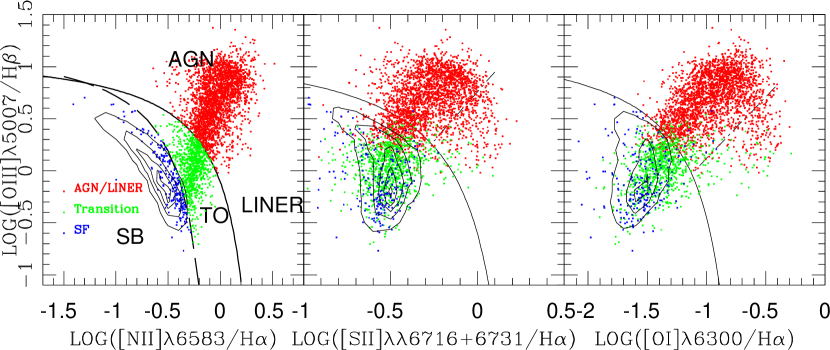
Figure 1: Three BPT diagnostic diagrams for the sub-samples. The AGNs, transition galaxies and star-forming galaxies with line widths $\sigma>2\sigma_{\mathrm{inst}}$ are plotted by the red, green and blue squares, respectively. The underlying density contours show the distributions on the three diagnostic diagrams for the star-forming galaxies with narrower emission-line widths, i.e., $\sigma<2\sigma_{\mathrm{inst}}$ The solid lines show the theoretical demarcation lines separating AGNs from star-forming galaxies proposed by Kewley et al. (2001), and the long-dashed line the empirical line proposed in Kauffmann et al. (2003).

The three diagnostic BPT diagrams are shown in Figure 1 for the final samples, in which the AGNs, transition galaxies and star-forming galaxies are symbolized by the red, green and blue solid squares, respectively. The contours represent the distributions of the star-forming galaxies in the comparison sample.

3 SPECTRAL ANALYSIS

3.1 Stellar Features Separation

The spectra of the selected objects are reduced and analyzed by our principal component analysis (PCA) pipeline (see Wang & Wei (2008) for details). At first, each spectrum is corrected for the Galactic extinction using the extinction law with $R_{V}=3.1$ (Cardelli et al. 1989), in which the color excess $E(B-V)$ is taken from the Schlegel, Finkbeiner, and Davis Galactic reddening map (Schlegel et al. 1998). Secondly, each extinctions-corrected spectrum is then transformed to the rest frame, along with the flux correction due to the relativity effect, given the redshift provided by the SDSS pipelines (Glazebrook et al. 1998; Bromley et al. 1998). The stellar absorption features are subsequently separated from each rest-frame spectrum by modeling the continuum and absorption features by the sum of the first seven eigenspectra. The eigenspectra are built from the standard single stellar population spectral library developed by Bruzual & Charlot (2003). Each of the spectra is fitted over the rest-frame wavelength range from 3700 to 7000Å by a $\chi^{2}$ minimization, except for the regions with strong emission lines (e.g., Balmer lines, [O III]$\lambda\lambda$4959, 5007, [N II]$\lambda\lambda$6548,6583, [S II]$\lambda\lambda$6716, 6731, [O II]$\lambda$3727, [O III]$\lambda$4363 and [O I]$\lambda$6300).

3.2 Emission-line Profile Measurements

3.2.1 Line profile parameters

The rest-frame emission-line isolated spectra are used to parametrize the spectral profiles of their [O III]$\lambda$5007 emission lines, after the stellar components are removed from the observed spectra. The emission-line profile can be parametrized by many possible ways. The widely used ones include the FWHM and the second moment of the line that is defined as

$$\sigma^{2}=\bigg{(}\frac{c}{\overline{\lambda}}\bigg{)}^{2}\frac{\int(\lambda-\overline{\lambda})^{2}f_{\lambda}d\lambda}{\int f_{\lambda}d\lambda}$$ (1)

where $\sigma$ is in units of $\rm km\ s^{-1}$, $\overline{\lambda}=\int\lambda f_{\lambda}d\lambda/\int f_{\lambda}d\lambda$ and $f_{\lambda}$ is the line centroid (i.e., the first moment) and the flux density of the continuum-subtracted line flux, respectively. For a pure Gaussian profile, we have a relationship $\mathrm{FWHM}=2\sqrt{2\ln 2}\sigma\approx 2.35\sigma$, which means that both FWHM and $\sigma$ comparably describe the line broadening if the line profile is a Gaussian function. However, as stated in Greene & Ho (2005), $\sigma$ contains more information on the line profile broadening if the profile deviates from a pure Gaussian profile.

Heckman et al. (1981) defined an asymmetry index $\rm{AI_{20}=(WL20-WR20)/(WL20+WR20)}$ to measure the line asymmetry of [O III] emission lines, where $\rm WL20$ and $\rm WR20$ is the half width to the left and right of the line center defined as the 80% peak intensity level. Basing upon the index $\rm{AI_{20}}$, the authors found that the blue asymmetry is shown in about 80% of the 36 Seyfert and radio galaxies. Alternatively, the asymmetry index $\rm A.I.=[C(\frac{3}{4})-C(\frac{1}{4})]/FWHM$ is widely used to measure the asymmetry of AGN’s broad emission lines, where $\rm C(i)$ are profile centroids measured at different levels (see review in Sulentic et al. 2000). In addition to the asymmetry, the emission-line shapes of AGNs vary from extremely peaked to very “boxy”. Previous studies used the ratio of line widths at different levels to parametrize such line shapes (e.g., Marziani et al. 1996).

To make the statistical study on [O III] line profile is feasible for a large sample, we adopt the high-order dimensionless line shape parameters to describe the line profile departures from a pure Gaussian function (see Binney & Merrifield (1998) for more details):

$$\xi_{k}=\mu_{k}/\sigma^{k}\ k\geq 3$$ (2)

where $\mu_{k}$ is the $k$-order moment defined as

$$\mu_{k}=\bigg{(}\frac{c}{\overline{\lambda}}\bigg{)}^{k}\int(\lambda-\overline{\lambda})^{k}f_{\lambda}d\lambda$$ (3)

and $\sigma$ is the second order moment defined in Eq (1), respectively. The first shape parameter $\xi_{3}$ is termed the “skewness” that measures the deviation from symmetry. A pure Gaussian profile corresponds to $\xi_{3}=0$. The emission-line shape with a positive value of $\xi_{3}$ shows a red asymmetry, and the shape with a negative value a blue asymmetry. The second parameter $\xi_{4}$ is termed the “kurtosis” that measures the symmetric deviation from a pure Gaussian profile (for a pure Gaussian profile, we have $\xi_{4}=3$). The emission line with peaked profile superposed on a broad base has a value of $\xi_{4}>3$. A value of $\xi_{4}<3$ corresponds to a “boxy” line profile. We refer the readers to Figure 11.5 in Binney & Merrifield (1998) for how the values of $\xi_{3}$ and $\xi_{4}$ vary with the line shapes.

3.2.2 Relative velocity shifts

The bulk relative velocity shift of the [O III] emission line is measured relative to the H$\beta$ emission line in each emission-line isolated spectrum, because the H$\beta$ line can be easily detected and because the line shows very small velocity shift relative to the galaxy rest-frame (e.g., Komossa et al. 2008). The velocity shift is calculated as $\Delta\upsilon=\delta\lambda/\lambda_{0}c$, where $\lambda_{0}$ and $c$ is the rest-frame wavelength of the [O III]$\lambda 5007$ emission line and the velocity of light, respectively. $\delta\lambda$ denotes the wavelength shift of the [O III] line with respect to the H$\beta$ line. The shift is determined from the measured line centroids ($\overline{\lambda}$) and the rest-frame wavelengths in vacuum of both lines. With the definition of the velocity shift, a blueshift corresponds to a negative value of $\Delta\upsilon$, and a redshift to a positive value.

3.3 Stellar Population Properties

By following our previous studies again, we use the two Lick indices, i.e., the 4000Å break ($D_{n}(4000)$) and the equivalent width of H$\delta$ absorption feature of A-type stars (H$\delta_{A}$), as the indicators of the ages of the stellar populations of the galaxies (e.g., Heckman et al. 2004; Kauffmann et al. 2003; Kauffmann & Heckman 2008; Kewley et al. 2006; Wang & Wei 2008, 2010; Wild et al. 2007). Both indices are measured in the removed stellar component for each spectrum, and are reliable age indicators until a few Gyr after the onset of a burst (e.g., Kauffmann et al. 2003, Bruzual & Charlot 2003).

3.4 Broad-Line AGNs

The sub-sample of partially obscured AGNs associated with broad H$\alpha$ emission lines (i.e., Seyfert 1.8/1.9 galaxies) is selected from the parent AGN and transition galaxy samples. Although the existence of the broad H$\alpha$ emission is direct indicative of the accretion activity of the central SMBH, the underlying AGN’s continuum in these partially obscured AGNs could potentially decrease the measured two indices. These partially obscured AGNs are therefore removed from the subsequent analysis when the two indices are involved.

Following our previous studies (Wang & Wei 2008), the broad-line AGNs are selected by the means of the high-velocity wings of the broad H$\alpha$ components on their blue side after the stellar features are removed from the spectra. The red wing is not adopted in the selection because of the superposition of the strong [N II]$\lambda$6583 emission line. The partially obscured AGNs are at first automatically selected by the criterion $F_{\mathrm{w}}/\sigma_{c}\geq 3$, where $F_{\mathrm{w}}$ is the specific flux of the line wing averaged within the wavelength range from 6500 to 6350Å in the rest-frame, and $\sigma_{c}$ is the standard deviation of the continuum flux within the emission-line free region ranging from $\lambda 5980$ and $\lambda 6020$. The automatically selected AGNs are then inspected one by one by eyes. In total, there are 174 broad-line Seyfert galaxies/LINERs and 55 broad-line transition galaxies.

3.5 Uncertainties estimation

The MPA/JHU catalog contains many duplicates because of the repeat observations. The duplicates allow us to roughly estimate the uncertainties for the line shape parameters and the stellar population age indicators. The duplicates are reduced and measured by the same method as described above. For the three main sub-samples (i.e., AGNs, transition galaxies and star-forming galaxies), the uncertainties are estimated to be $0.14\pm 0.08$ and $0.20\pm 0.14$ for the shape parameters $\xi_{3}$ and $\xi_{4}$, respectively. The two Lick indices have uncertainties: $\Delta D_{n}(4000)=0.03\pm 0.02$, and $\Delta$H$\delta_{A}=0.38\pm 0.19$. For the comparison sample, the duplicates provide the uncertainties of $0.08\pm 0.05$ and $0.13\pm 0.06$ for the parameters $\xi_{3}$ and $\xi_{4}$, respectively.

4 ANALYSIS AND RESULTS

After obtaining all the required parameters, the relation between the [O III] line profiles and the stellar population properties is examined in this section.

4.1 [O III] Line Width and [O III]$\lambda 5007$ Relative Velocity Shifts: AGNs versus Transition Galaxies

The [O III] line profile is compared between the AGNs and the transition galaxies in this section. To avoid the possible systematics caused by the host galaxy properties, we compare the line profiles in a sample of matched galaxy pairs (e.g., Kauffmann et al. 2006). The matched pairs are created according to the SDSS DR4 MPA/JHU AGN catalog. The catalog provides the measurements of galaxy properties for the AGNs that are classified according to the demarcation line given in Kauffmann et al. (2003). We select the pairs that have $\Delta\log M_{*}<0.1$, $\Delta\log\mu_{*}<0.1$, $\Delta C<0.1$, $\Delta\sigma_{*}<30\ \mathrm{km\ s^{-1}}$, and $\Delta z<0.01$, where $M_{*}$ is the stellar mass in unit of $M_{\odot}$, $\mu_{*}$ is the effective stellar mass-density ($\mu_{*}=M_{*}/2\pi r^{2}_{\mathrm{50,z}}$, where $r_{\mathrm{50,z}}$ is the half-light radius in the $z$-band) in unit of $M_{\odot}\ \mathrm{kpc^{-2}}$, $C$ is the concentration index defined as $C=R_{90}/R_{50}$ the ratio of the radius enclosing 90% of the total flux to that enclosing 50% of the flux in the $r$-band, $\sigma_{*}$ is the stellar velocity dispersion and $z$ is the redshift. Because there are much more AGNs than the transition galaxies in our sample, a large fraction of the transition galaxies have a few of AGN pairs. In these cases, one AGN is assigned to a pair by a random selection, and the final distributions are built from 100 Monte-Carlo iterations. Finally, there are totally 163 distinct galaxy pairs, in which no galaxy is assigned to a pair more than once.

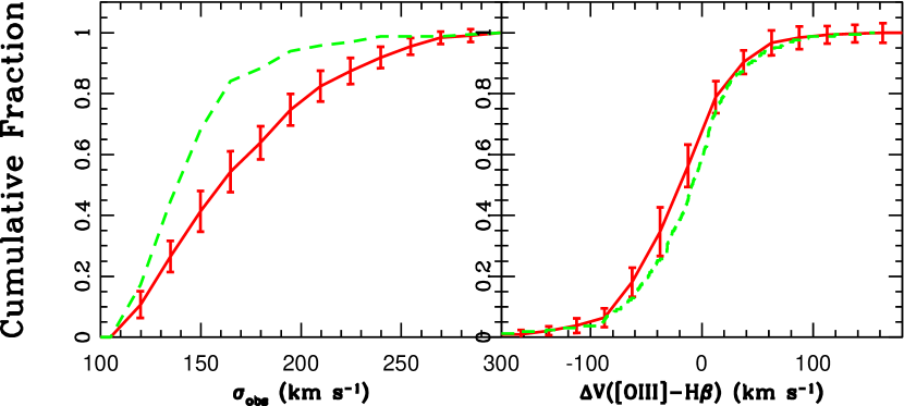
Figure 2: Left panel: Cumulative distributions of the measured line widths of the [O III] emission lines for the AGNs (the red-solid line) and the transition galaxies (the green-dotted line). Right panel: The same as the left panel but for the measured relative velocity shifts

The left panel in Figure 2 compares the cumulative distributions of the [O III] line widths in terms of the calculated velocity dispersions. The AGNs and transition galaxies are shown by the red-solid and green-dotted lines, respectively. The error-bars are resulted from our iterations. One can see clearly that the line profiles of the AGNs are systematically wider than that of the transition galaxies. A two-side Kolmogorov Smirnov test yields a maximum discrepancy of 0.282 with a corresponding probability that the two samples match of $4.6\times 10^{-5}$. In fact, the comparison of the parameter $\xi_{4}$ indicates that the difference in the distributions is likely due to the fact that the transition galaxies have systematically smaller values of $\xi_{4}$ than the AGNs (see section 4.3 for more details). That means the transition galaxies are associated with weaker [O III] broad components compared to the AGNs, which implies that the feedback caused by the material outflow is less stronger in the transition galaxies than in the AGNs.

The distributions of the [O III]$\lambda 5007$ relative velocity shifts defined in Section 3.2.2 are compared in the right panel of Figure 2 between the AGNs and transition galaxies. The symbols are the same as the left panel. A two-side Kolmogorov Smirnov test shows that the two samples are matched at a probability of 77%, although a careful examination suggests that the AGNs marginally tend to be associated with larger negative velocity shifts compared with the transition galaxies.

4.2 Line Shape Parameters $\xi_{3}$ and $\xi_{4}$

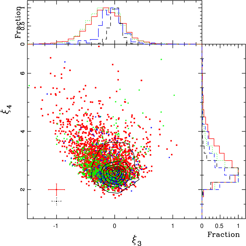
Figure 3: Bottom-left panel: $\xi_{4}$ versus $\xi_{3}$ diagram for all the sub-samples. The AGNs and transition galaxies are presented by the red and green points, respectively. The blue points are plotted for the star-forming galaxies with [O III] line widths $\sigma>2\sigma_{\mathrm{inst}}$. The over-plotted black contours show the distribution for the star-forming galaxies in the comparison sample with $\sigma<2\sigma_{\mathrm{inst}}$. The red-solid cross and the black-dashed cross at the left-bottom corner indicates the uncertainties for the large line-width samples and the comparison sample, respectively. The uncertainties are estimated from the duplicates. Upper-left panel: distributions of the parameter $\xi_{3}$ for the four sub-samples (AGNs: red solid line, transition galaxies: green dotted line, star-forming galaxies with $\sigma>2\sigma_{\mathrm{inst}}$: blue long-dashed line, and star-forming galaxies with $\sigma<2\sigma_{\mathrm{inst}}$: black short-dashed line). Bottom-right panel: The same as the upper-left panel but for the parameter $\xi_{4}$.

The left-bottom panel in Figure 3 shows the $\xi_{4}$ versus $\xi_{3}$ diagram. The AGNs, transition galaxies and star-forming galaxies are symbolized by the red, green and blue points, respectively. The over-plotted contours present the distribution of the star-forming galaxies in the comparison sample. The two crosses at the left-bottom corner show the typical uncertainties for both parameters as roughly estimated from the duplicates. The red-solid one indicates the uncertainties for the large line-width objects, and the black-dashed one for the comparison sample. The left-upper panel and the right-bottom panel shows the distributions of the parameters $\xi_{3}$ and $\xi_{4}$ for all the sub-samples (including the comparison sample), respectively. The distributions are color-codded for the sub-samples as same as the left-bottom panel. As expected from an emission-line profile dominated by the instrumental resolution, the distribution of the comparison sample is strongly clustered around the point (i.e., $\xi_{3}=0$ and $\xi_{4}=3$) associated with a pure Gaussian function. The last column in Table 1 lists the average and median values of $\xi_{3}$ ($\overline{\xi}_{3}=0.01$ and $\langle\xi_{3}\rangle=0.01$) for the comparison sample. The same values are listed in the last column in Table 2 but for the parameter $\xi_{4}$ ($\overline{\xi}_{4}=2.61$ and $\langle\xi_{4}\rangle=2.58$). The dispersions is calculated to be 0.14 and 0.43 for the parameters $\xi_{3}$ and $\xi_{4}$, respectively. The distribution therefore validates our spectral measurements because the distribution of the comparison sample is highly consistent with the prediction of a pure Gaussian function.

Similar as the comparison sample, the statistics are tabulated in Table 2 and 3 for both AGNs and transition galaxies as well. One can find from the tables that the line profiles of these galaxies systematically deviate from that of the control sample (i.e., deviate from a pure Gaussian profile) by not only smaller $\xi_{3}$ (i.e., a stronger blue asymmetry), but also larger $\xi_{4}$ (i.e., a stronger broad base). The main panel in Figure 3 shows that both AGNs and transition galaxies form a sequence starting from the pure Gaussian region to the upper-left corner. In fact, this phenomenon is qualitatively in agreement with the fact that two Gaussian components, one representing the narrow line core and the other representing the blueshifted broad wing, are usually required to model the observed [O III] line profiles. A minor fraction of the objects deviate from the sequence by their positive values of $\xi_{3}$. By inspecting the spectra of these objects one by one by eyes, we find that the deviations are mainly resulted from the contamination at the [O III] red wing caused by the weak low-ionization emission line He I$\lambda$5016 (Veron et al. 2002).

It is interesting to see that the star-forming galaxies with $\sigma>2\sigma_{\rm inst}$ follow the sequence as well, although most of them have Gaussian line profiles. In order to validate the deviations in these galaxies, the spectra with $\xi_{3}<-0.5$ are then inspected one by one by eyes again. To understand the nature of these star-forming galaxies with blue asymmetric [O III] emission lines, we need to carefully model all the strong emission lines in individual spectrum. The issue is out of the topic of this paper, and will be examined in our subsequent studies.

The results from the two-sides Kolmogorov-Smirnov tests are tabulated in Table 3 and 4 for the parameters $\xi_{3}$ and $\xi_{4}$, respectively. Each entry contains the maximum absolute discrepancy between the used two sub-samples, and the corresponding probability that the two sub-samples match. Although the AGNs and the transition galaxies show similar distributions for $\xi_{3}$, the AGNs significantly differ from the transition galaxies in the distribution of parameter $\xi_{4}$. The fraction of objects with strong broad [O III] wings is larger in the AGNs than in the transition galaxies

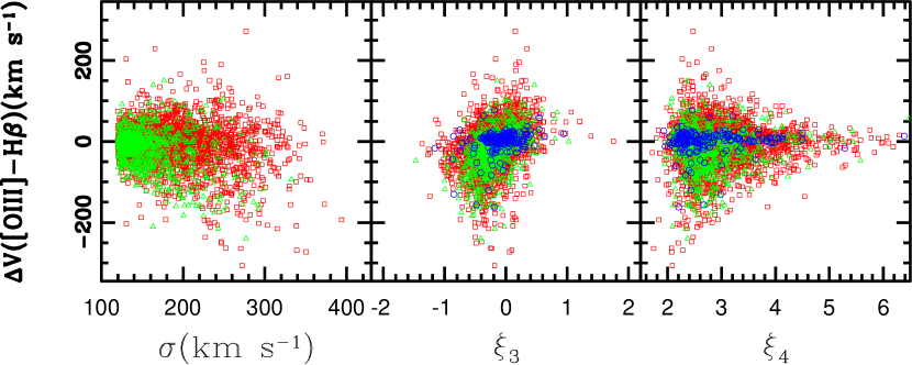
Figure 4: Relative velocity shift $\Delta\upsilon$ plotted against line width $\sigma$ (left panel), parameters $\xi_{3}$ (middle panel) and $\xi_{4}$ (right panel). In each panel, the AGNs and transition galaxies are plotted by the red and green points, respectively. The star-forming galaxies with $\sigma\geq 2\sigma_{\mathrm{inst}}$ are marked by the blue points.

Previous studies frequently identified a strong correlation between the [O III] line widths and the [O III] blueshifts (e.g., Bian et al. 2005; Komossa et al. 2008; Zamanov et al. 2002). The correlation is commonly explained by the material outflows. The similar correlations are also identified in iron coronal lines (Erkens et al. 1997) and optical Fe II complex (Hu et al. 2008) in typical type I AGNs. The left panel in Figure 4 plots the velocity shift as a function of the line width for the AGNs (red points) and the transition galaxies (green points). Spearman rank-order tests show a marginal anti-correlation between the velocity shifts and the line widths for the AGNs (with a Spearman correlation coefficient $r_{s}=-0.088$ at a significance level $P<10^{-4}$, where $P$ is the probability that there is no correlation between the two variables.), and, however, a stronger correlation for the transition galaxies (with $r_{s}=-0.229$ and $P<10^{-4}$). As an additional examination, the middle panel in the figure plots the velocity shift against the parameter $\xi_{3}$. Strong correlations between the two variables can be identified for both AGNs ($r_{s}=0.334$ and $P<10^{-4}$) and transition galaxies ($r_{s}=0.513$ and $P<10^{-4}$), which means that larger the blueshift, stronger the blue asymmetry. One can see from the correlations that the objects with the largest velocity shifts deviate from the correlations. These objects instead show symmetrical line profiles. In order to further describe their line profiles, the right panel in the figure plots the velocity shift against the parameter $\xi_{4}$. We find that these [O III] lines have “boxy” line profiles rather than peaked ones. In fact, a “boxy” line profile could be reproduced by the sum of two or more (distinct) peaks with comparable fluxes and line widths (see examples of spectra in the Figure 1 in Greene & Ho 2005).

4.3 [O III] Line Profile versus Stellar Population

The evolution effect on the [O III] line profile is examined in this section by using the two indices, $D_{n}(4000)$ and H$\delta_{\mathrm{A}}$, as the indicators of the ages of the circumnuclear stellar populations. As described in Section 3.3, the partially obscured AGNs are excluded from the analysis throughout this section.

The two indices are plotted against the parameter $\xi_{3}$ (the left panels) and against the relative velocity shift (the right panels) for the AGNs in Figure 5. At the first glance of the four panels, we fail to directly identify any significant correlation between the line profile parameters and the stellar population ages. To examine the evolution effect in more details, we divide the AGN sample into two groups according to their $\xi_{3}$ values: one group for the galaxies with $\xi_{3}>-0.5$ and the another one for the galaxies with $\xi_{3}<-0.5$. The distributions of the $D_{n}(4000)$ values are compared between the two groups in the upper-left panel of Figure 7. The comparison indicates a significant difference between the two groups. The AGNs with larger amount of blue asymmetry are systematically associated with younger stellar populations. A two-sides Kolmogorov Smirnov test indicates that the difference between the two distributions is at a significance level $P<1\times 10^{-9}$ with a maximum absolute discrepancy of 0.22. Similar as the parameter $\xi_{3}$, the AGN sample is instead separated into two groups by the relative velocity shift at $\Delta\upsilon=-100\ \mathrm{km\ s^{-1}}$. We identify a marginal trend that larger the blue velocity shifts, younger the associated stellar populations (see the bottom-left panel in Figure 7). The same statistical test yields a probability that the two groups match of $P=9\times 10^{-2}$ (with a maximum absolute discrepancy of 0.11).

Figure 6 is the same as Figure 5 but for the transition galaxies. The same methods as the AGN sample are adopted to divide these galaxies into two groups. The right panels in Figure 7 compare the distributions of $D_{n}(4000)$ between the two groups. The two-sides Kolmogorov-Smirnov tests suggest that the two distributions match at the probabilities $P=0.02$ for the $\xi_{3}$ separation and $P=0.32$ for the $\Delta\upsilon$ separation, which is much less significant than the AGN sample. In fact, these results are easily understood because the transition galaxies are usually systematically younger than the AGNs (see also in Kewley et al. 2006; Schawinski et al. 2007; Wang & Wei 2008).

In summary, our results indicate that the AGNs associated with young stellar populations show a wide range in their [O III] line profiles that vary from a blue asymmetrical shape to a Gaussian function. In contrast, the AGNs associated with old stellar populations always show symmetrical line profiles.

5 DISCUSSIONS

5.1 $L/L_{\mathrm{Edd}}$ as A Physical Driver

The evolution of [O III]$\lambda$5007 emission-line profile is studied by using a large sample of narrow emission-line galaxies selected from the MPA/JHU SDSS DR7 catalog. The line-profile parameterizing allows us to reveal a trend that AGNs with more significant blue asymmetries tend to be associated with younger stellar populations. At the beginning of discussion, we argue that the trend is not driven only by the orientation effect (Antonucci 1993; Elitzur 2007). It is widely accepted that the commonly observed blue asymmetrical and blue-shifted [O III] line profiles are caused by the wind-driven NLR outflows. The orientation-driven scenario therefore results in an odd corollary that a fraction of the AGNs with young stellar populations have outflow directions closer to the line-of-sight of observers than the AGNs with old stellar populations, while the starlight components from the host galaxies are believed to be isotropic.

The revealed trend can be alternatively driven by the activity of the central SMBH. In fact, there is many observational evidence supporting that the [O III] line blue asymmetries and blueshifts are correlated with $L/L_{\mathrm{Edd}}$ or Eigenvector-I space in typical type I AGNs (see the description and citations in Section 1). The relationship between the [O III] line profile and $L/L_{\mathrm{Edd}}$ is examined in the current narrow-line AGN sample to present a complete understanding. Similar as the previous studies of narrow-line AGNs, the parameter $L_{\mathrm{[OIII]}}/\sigma_{*}^{4}$ (e.g., Heckman et al. 2004) is used as a proxy of $\lambda_{\mathrm{Edd}}=L/L_{\mathrm{Edd}}$, where $L_{\mathrm{[OIII]}}$ and $\sigma_{*}$ is the [O III]$\lambda 5007$ line luminosity and the bulge velocity dispersion, respectively. The transition galaxies are excluded from the subsequent calculations because of the possible contamination caused by H II regions. The bolometric luminosity $L$ is transformed from $L_{\mathrm{[OIII]}}$ through the bolometric correction $L/L_{\mathrm{[OIII]}}\approx 3500$ (see Heckman et al. (2004) for details). By assuming the Balmer decrement for the standard Case B recombination and the Galactic extinction curve with $R_{V}=3.1$, the [O III] line luminosity is corrected for the local extinction that is inferred from the narrow-line ratio $\mathrm{H\alpha/H\beta}$. The blackhole mass is estimated from the $M_{\mathrm{BH}}-\sigma_{*}$ calibration: $\log(M_{\mathrm{BH}}/M_{\odot})=8.13+4.02\log(\sigma_{*}/200\ \mathrm{km\ s^{-1}})$ (Tremaine et al. 2002), in which the velocity dispersion is measured for each spectrum through our PCA fittings. The galaxies with $\sigma_{*}<70\ \mathrm{km\ s^{-1}}$ are removed from the analysis because the SDSS instrumental resolution is $\sigma_{\mathrm{inst}}\approx 65\ \mathrm{km\ s^{-1}}$.

The results are shown in Figure 8. The left panel presents an anti-correlation between $L_{\mathrm{[OIII]}}/\sigma_{*}^{4}$ and $D_{n}(4000)$. Larger the Eddington ratio, and younger the stellar population, which is consistent with the previous studies (e.g., Kewley et al. 2006; Kauffmann et al. 2007). The middle panel plots $L_{\mathrm{[OIII]}}/\sigma_{*}^{4}$ as a function of the parameter $\xi_{3}$. When compared with Figure 5, one can find a similar trend in the $L_{\mathrm{[OIII]}}/\sigma_{*}^{4}$ vs. $\xi_{3}$ plot as that in the $D_{n}(4000)$ vs. $\xi_{3}$ plane. AGNs with large amount of blue asymmetry tend to have large $L/L_{\mathrm{Edd}}$. A much stronger trend can be identified in the right panel between $L_{\mathrm{[OIII]}}/\sigma_{*}^{4}$ and the parameter $\xi_{4}$. The trend indicates a fact that AGNs with larger Eddington ratios tend to be associated with stronger [O III] broad components. However, we fail to find a significant trend between $L_{\mathrm{[OIII]}}/\sigma_{*}^{4}$ and the bulk relative velocity shifts $\Delta\upsilon$.

Spearman rank-order tests are performed to show either the Eddington ratio or the stellar population is intrinsically related with the line asymmetry. The resulted correlation coefficient matrix is listed in Table 5. All the entries in the table have a probability of null correlation $P<10^{-4}$. Although both $\lambda_{\mathrm{Edd}}$ and $D_{n}(4000)$ are correlated with $\xi_{3}$ at comparable significance levels, $\xi_{4}$ is more strongly correlated with $\lambda_{\mathrm{Edd}}$ than with $D_{n}(4000)$. The stronger correlation therefore indicates that the trend between the line asymmetry and $D_{n}(4000)$ is likely driven physically by the evolution of the Eddington ratio (see below).

5.2 Evolution of [O III] Emission-line Profile

The trend that AGNs with more significant blue asymmetry tend to be associated with younger stellar populations provides a piece of direct evidence supporting the co-evolution of the NLR kinematics and the growth of the host galaxy. AGNs with stronger outflows tend to be at their earlier evolutionary stage as inferred from the stellar population ages. The analysis in the above section further suggests that the trend is likely driven by $L/L_{\mathrm{Edd}}$. The important evolutionary role of $L/L_{\mathrm{Edd}}$ has been frequently proposed in recent studies (e.g., Wang & Wei 2008, 2010; Kewley et al. 2006; Heckman et al. 2004). Putting these pieces together yields an improved co-evolution scenario in which AGN likely evolve from a high-$L/L_{\rm Edd}$ state with strong outflow to a low-$L/L_{\rm Edd}$ state with weak outflow as the circumnuclear stellar population continually ages.

This evolutionary scenario is consistent with the current understandings of AGNs. Lieghly et al. (1997) reported evidence of relativity outflows in three NLS1s. In comparison with typical broad-line Seyfert galaxies, NLS1s are “young” AGNs (Mathur 2000) typical of smaller $M_{\mathrm{BH}}$, higher $L/L_{\rm Edd}$, larger [O III] emission-line asymmetries, younger circumnuclear stellar populations possibly at post-starburst phase, and enhanced star formations as recently revealed by the observation of Spitzer (e.g., Boroson 2005; Zamanov et al. 2002; Boroson & Green 1992; Wang et al. 1996; Boller et al. 1996; Sulentic et al. 2000; Boroson 2002; Xu et al. 2007; Zhou et al. 2005; Wang & Wei 2006). In addition to the observational ground, the feedback from central AGN is frequently involved in the modern numerical and sim-analytical galaxy evolution models to quench the star formation and to blow the gas or dust away through the powerful AGN’s wind (e.g., Springel et al. 2005; di Matteo et al. 2005; Kauffmann & Heckman 2008; Fabian 1999; Hopkins et al. 2005, 2008a,b; Croton et al. 2006; Somerville et al. 2008; Khalatyan et al. 2008). The numerical simulation done by Hopkins et al. (2005) suggests a scenario that the powerful AGN’s wind is required to occur in the young AGN phase in which the central SMBH is heavily obscured by the starforming gas and dust.

5.3 Are Transition Galaxies at Intermediate Evolutionary Phase?

Transition galaxies are the narrow emission-line galaxies located between the theoretical and empirical demarcation lines in the [O III]/H$\beta$ versus [N II]/H$\alpha$ diagnostic diagram (Kauffmann et al. 2003; Kewley et al. 2001). Their emission-line properties are explained by the mixture of the contributions from both star formations and typical AGNs (e.g., Kewley et al. 2006; Ho et al. 1993, see recent review in Ho 2008). Our spectral profile analysis indicates that the transition galaxies differs from the Seyfert galaxies in their [O III] emission-line profiles. The transition galaxies systematically show weaker [O III] broad wings, and narrower [O III] line widths than the Seyfert galaxies, which implies that the two kinds of objects are different from each other in their mass outflow kinematics. The line profile comparison allows us to suspect that the transition galaxies “bridge” the AGN-starburst co-evolution from early starburst-dominated phase to late AGN-dominated phase (e.g., Yuan et al. 2009; Wang & Wei 2006; Schawinski et al. 2007, 2009). The evolutionary role of the transition galaxies has been reported in the recent studies by many authors. With the large SDSS spectroscopic database, transition galaxies are found to be systematically associated with younger stellar populations than Seyfert galaxies (e.g., Kewley et al. 2006; Wild et al. 2007; and also see Figure 6 in this paper). Westoby et al. (2007) found that the distribution of the H$\alpha$ equivalent widths of the transition galaxies peaks at the valley between the red and blue sequences. By analyzing the mm-wavelength observation taken by the 30m IRAM, Schawinski et al. (2009) suggested that molecular gas reservoir is destructed by the AGN feedback at early AGN+starforming transition phase.

6 Conclusion

We systematically examined the evolutionary issue of the [O III]$\lambda 5007$ emission-line profile by using a large sample of narrow emission-line galaxies selected from the MPA/JHU SDSS DR7 value-added catalog. The sample is separated into three sub-samples (i.e., star-forming galaxies, transition galaxies and Seyfert galaxies/LINERs) basing upon the line ratios given in the catalog. Two shape parameters, skewness ($\xi_{3}$) and kurtosis ($\xi_{4}$), are additionally used to quantify the profile deviation from a pure Gaussian. Our analysis indicates that a) the transition galaxies are systematically associated with narrower line widths and with weaker [O III] broad wings than the AGNs; b) the AGNs with stronger blue asymmetries tend to be associated with younger stellar populations. The evolutionary significance of the [O III] line profile suggests a co-evolution of the outflow feedback and the AGN’s host galaxy.

Appendix A Appendix

A toy model of emission-line profile is constructed here to illustrate the effect of the instrumental resolution on the measured line shape parameters. The model is constructed by assuming an observed [O III] emission line profile that is prescribed by the sum of two pure Gaussian profiles: $\phi(\upsilon)=\phi_{1}(0,\sigma_{1})+\alpha\phi_{2}(\mu,\sigma_{2})$, where $\phi_{1}(0,\sigma_{1})$ is a normalized Gaussian distribution with the peak at zero and the variance of $\sigma^{2}_{1}$, $\phi_{2}(\mu,\sigma_{2})$ is the same distribution but with the peak shifted at $\mu$ and the variance of $\sigma^{2}_{2}$, and $\alpha$ is a parameter much less than unit. With this two Gaussian components model, $\phi_{1}(0,\sigma_{1})$ represents the narrow core of the emission, and $\alpha\phi_{2}(\mu,\sigma_{2})$ the shifted, low-contrast broad wing (We require $|\mu|/\sigma_{i}\ll 1$ for avoiding double peaked profile). The normalizations of the two distributions yield $\int\phi(\upsilon)d\upsilon=1+\alpha$.

The first moment (i.e., the line centroid) is written as $\overline{\mu}=\int\upsilon\phi d\upsilon=\int\upsilon\phi_{1}d\upsilon+\alpha\int\upsilon\phi_{2}d\upsilon=\alpha\mu$, which is not affected by the instrumental resolution. With the first moment, the high-order moments are written as

$$E\{(\upsilon-\overline{\mu})^{p}\}=\int(\upsilon-\overline{\mu})^{p}\phi d\upsilon$$ (A1)

The second moment of the total line profile is therefore inferred to be approximately the linear combination of the square of the second moments of the two distributions: $\int(\upsilon-\overline{\mu})^{2}\phi d\upsilon=\sigma^{2}_{1}+\alpha\sigma^{2}_{2}+\mu^{2}\alpha(1-\alpha)^{2}\approx\sigma^{2}_{1}+\alpha\sigma^{2}_{2}$. In the context of the toy model, the linear combination means that the instrumental resolution $\sigma_{\mathrm{inst}}$ can be removed from the measured values according to the equation $\sigma^{2}_{\mathrm{obs}}=\sigma^{2}+(1+\alpha)\sigma^{2}_{\mathrm{inst}}$, which means that the removal depends on the relative strength of the low-contrast Gaussian profile, i.e., the parameter $\alpha$.

The third moment of the total profile can be trivially obtained through the integration $\int(\upsilon-\overline{\mu})^{3}\phi d\upsilon=(\alpha-3\alpha^{2}+2\alpha^{3}-\alpha^{4})\mu^{3}+3\mu\alpha(\sigma^{2}_{2}-\sigma^{2}_{1}-\alpha\sigma^{2}_{2})$. By ignoring the terms with high-orders of $\alpha$, the third moment approximately equals to $\approx\alpha\mu^{3}+3\alpha\mu(\sigma^{2}_{2}-\sigma_{1}^{2})$. The result suggests that the measured third moment depends not only on the relative shift of the low-contrast Gaussian profile, but also on the relative strength denoted by the parameter $\alpha$. Although the second term in the above result means that the third moment does not depend on the instrumental resolution in our toy model at the first order approximation: $\sigma_{2}^{2}-\sigma_{1}^{2}=\sigma_{\mathrm{obs,2}}^{2}-\sigma_{\mathrm{obs,1}}^{2}$, the definition of the dimensionless shape parameter $\xi_{3}$ introduces a non-linear dependence on the instrumental resolution in the denominator (see Eq. 2 in the main text). By adopting the same approach, the fourth moment is calculated to be $\int(\upsilon-\overline{\mu})^{4}\phi d\upsilon\approx\alpha\mu^{4}+3(\sigma^{4}_{1}+\alpha\sigma^{4}_{2})+6\alpha\mu^{2}\sigma^{2}_{2}$, where one sees that the second and third terms introduce again a non-linear dependence on the instrumental resolution.

With this toy model, the galaxies whose [O III]$\lambda$5007 lines are narrower than 2$\sigma_{\mathrm{inst}}$ are then dropped out from our statistical analysis in order to avoid the effect of the instrumental resolution on the measured line shape parameters.

Figure 5: Left column: stellar population properties (i.e., the indices of $D_{n}(4000)$ and H$\delta_{\mathrm{A}}$) plotted against the line shape parameter $\xi_{3}$ for the AGNs. Right column: both indices plotted against the relative velocity shift of the [O III] emission line for the AGNs.

Figure 6: The same diagram as Figure 5 but for the transition galaxies.

Figure 7: The distributions of $D_{n}(4000)$ are compared between the two groups with different [O III] line shape parameters (i.e., $\xi_{3}$ for the upper raw), and between the two groups with different relative velocity shifts (i.e., $\Delta V$([O III]-H$\beta$) for the bottom raw) for the AGNs (left column) and the transition galaxies (right column). In each panel, the solid line represents the objects with $\xi_{3}>-0.5$ (the upper raw) or $\Delta V>-100\ \mathrm{km\ s^{-1}}$ (the bottom raw), and the dashed one the objects with $\xi_{3}<-0.5$ or $\Delta V<-100\ \mathrm{km\ s^{-1}}$.

Figure 8: $L_{\mathrm{[OIII]}}/\sigma_{*}^{4}$ is plotted as a function of $D_{n}(4000)$ (left panel), the line profile parameters $\xi_{3}$ (middle panel) and $\xi_{4}$ (right panel) for the AGN sample.

Table 1: Statistical properties of the shape parameter $\xi_{3}$ for all the sub-samples.

Property	AGNs	Transitions	SF galaxies/$>2.0\sigma$	SF galaxies/$<2.0\sigma$
(1)	(2)	(3)	(4)	(5)
Numbers	2333	793	190	5843
$\overline{\xi}_{3}$	-0.167	-0.170	-0.09	0.01
$\langle\xi_{3}\rangle$	-0.165	-0.167	-0.08	0.01
$\sigma_{\xi_{3}}$	0.31	0.28	0.32	0.14

Table 2: Statistical properties of the shape parameter $\xi_{4}$ for all the sub-samples.

Property	AGNs	Transitions	SF galaxies/$>2.0\sigma$	SF galaxies/$<2.0\sigma$
(1)	(2)	(3)	(4)	(5)
Numbers	2333	793	190	5843
$\overline{\xi}_{4}$	3.00	2.79	2.84	2.61
$\langle\xi_{4}\rangle$	2.83	2.64	2.56	2.58
$\sigma_{\xi_{4}}$	0.70	0.56	1.01	0.43

Table 3: Two-sides Kolmogorov-Smirnov test matrix for the shape parameter $\xi_{3}$.

Sub-sample	AGNs	Transitions	SF galaxies/$>2.0\sigma$
	(1)	(2)	(3)
AGNs	-	0.034(0.48)	0.159($2.9\times 10^{-4}$)
Transitions	-	-	0.164($5.0\times 10^{-4}$)
SF galaxies/$>2.0\sigma$	-	-	-

Table 4: Two-sides Kolmogorov-Smirnov test matrix for the shape parameter $\xi_{4}$.

Sub-sample	AGNs	Transitions	SF galaxies/$>2.0\sigma$
	(1)	(2)	(3)
AGNs	-	0.154($<10^{-9}$)	0.214($2.0\times 10^{-7}$)
Transitions	-	-	0.133($9.0\times 10^{-3}$)
SF galaxies/$>2.0\sigma$	-	-	-

Table 5: Spearman Rank-order Correlation Coefficient Matrix for the AGNs

Property	$D_{4000}$	$\lambda_{\mathrm{Edd}}$
	(1)	(2)
$\xi_{3}$	0.218	-0.204
$\xi_{4}$	-0.292	0.449

References

- Abazajian et al. (2009) Abazajian, K. N., et al. 2009, ApJS, 182, 543
- Aoki et al. (2005) Aoki, K., Kawaguchi, T., & Ohta, K. 2005, ApJ, 618, 601
- Antonucci (1993) Antonucci, R. R. J. 1993, ARA&A, 31, 473
- Arribas et al. (1996) Arribas, S., Mediavilla, E., & Garcia-Lorenzo, B. 1996, ApJ, 463, 509
- Baldwin et al. (1981) Baldwin, J. A., Phillips, M. M., & Terlevich, R. 1981, PASP, 93, 5
- Balogh et al. (1999) Balogh, M. L., et al., 1999, ApJ, 527, 54
- Bian et al. (2005) Bian, W. H., Yuan, Q. R., & Zhao, Y. H. 2005, MNRAS, 364, 187
- Binney & Merrifield (1998) Binney, J., & Merrifield, M. 1998, Galactic Astronomy, Princeton, New Jersey
- Boller et al. (1996) Boller, T., Brandt, W. N., & Fink, H. 1996, A&A, 305, 53
- Boroson (2002) Boroson, T. A. 2002, ApJ, 565, 78
- Boroson (2003) Boroson, T. A. 2003, ApJ, 585, 647
- Boroson (2005) Boroson, T. A. 2005, AJ, 130, 381
- Boroson & Green (1992) Boroson, T. A., & Green, R. F. 1992, ApJS, 80, 109
- Bromley et al. (1998) Bromley, B. C., et al. 1998, ApJ, 505, 25
- Bruzual (1983) Bruzual, A. G. 1983, ApJ, 273, 105
- Bruzual & Charlot (2003) Bruzual, G., & Charlot, S. 2003, MNRAS, 344, 1000
- Cardelli et al. (1989) Cardelli, J. A., Clayton, G. C., & Mathis, J. S., 1989, ApJ, 345, 245
- Christopoulou et al. (1997) Christopoulou, P. E., Holloway, A. J., Steffen, W., Mundell, C. G., Thean, A. H. C., Goudis, C. D., Meaburn, J., & Pedlar, A. 1997, MNRAS, 284, 385
- Crenshaw & Kraemer (2000) Crenshaw, D. M., & Kraemer, S. 2000, ApJ, 532, 101
- Crenshaw et al. (2000) Crenshaw, D. M., et al. 2000, AJ, 120, 1731
- Crenshaw et al. (2010) Crenshaw, D. M., Schmitt, H. R., Kraemer, S. B., Mushotzky, R. F., & Dunn, J. P. 2010, ApJ, 708, 419
- Croton et al. (2006) Croton, D. J., et al. 2006, MNRAS, 365, 11
- Das et al. (2005) Das, V., et al. 2005, AJ, 130, 945
- Das et al. (2006) Das, V., Crenshaw, D. M., Kraemer, S. B., & Deo, R. P. 2006, AJ, 132, 620
- Das et al. (2007) Das, V., Crenshaw, D. M., & Kraemer, S. B. 2007, ApJ, 656, 699
- Davies et al. (2007) Davies, R., Mueller Sanchez, F., Genzel, R., Tacconi, L., Hicks, E., Friedrich, S., & Sternberg, A. 2007, ApJ, 671, 1388
- de Robertis & Osterbrock (1984) de Robertis, M. M., & Osterbrock, D. E. 1984, ApJ, 286, 171
- Di Matteo e tal. (2005) Di Matteo, T., Springel, V., & Hernquist, L. 2005, Nature, 433, 604
- Elitzur (2007) Elitzur, M. 2007, in ASP Conf. Ser. 373, The Central Engine of Active Galactic Nuclei, ed. L. C. Ho & J. -M. Wang (San Francisco, CA: ASP), 415
- Erkens et al. (1997) Erkens, U., Appenzeller, I., & Wagner, S. 1997, A&A, 323, 707
- Fabian (1999) Fabian, A. C. 1999, MNRAS, 308, L39
- Ferrarese & Merritt (2000) Ferrarese, L., & Merritt, D. 2000, ApJ, 539, 9
- Fischer et al. (2011) Fischer, T. C., Crenshaw, D. M., Kraemer, S. B., Schmitt, H. R., Mushotsky, R. F., & Dunn, J. P. 2011, ApJ, 727, 71
- Fischer et al. (2010) Fischer, T. C., Crenshaw, D. M., Kraemer, S. B., Schmitt, H. R., & Trippe, M. L. 2010, AJ, 140, 577
- Gebhardt et al. (2000) Gebhardt, K. et al. 2000, ApJ, 539, 13
- Glazebrook et al. (1998) Glazebrook, K., Offer, A., R., & Deeley, K. 1998, ApJ, 492, 98
- Granato et al. (2004) Granato, G. L., De Zotti, G., Silva, L., Bressan, A., & Danese, L. 2004, ApJ, 600, 580
- Greene & Ho (2005) Greene, J. E., & Ho, L. C. 2005, ApJ, 627, 721
- Grupe et al. (1999) Grupe, D., Beuermann, K., Mannheim, K., & Thomas, H, -C. 1999, A&A, 350, 805
- Grupe & Mathur (2004) Grupe, D., & Mathur, S. 2004, ApJ, 606, 41
- Haring & Rix (2004) Haring, N., & Rix, H. W. 2004, ApJ, 604, 89
- Hasinger et al. (2005) Hasinger, G., Miyaji, T., & Schmidt, M. 2005, A&A, 441, 417
- Heckman (1981) Heckman, T. M. 1981, ApJ, 250, 59
- Heckman & Kauffman (2006) Heckman, T. M., & Kauffmann, G. 2006, NewAR, 50, 677
- Heckman et al. (2004) Heckman, T. M., Kauffmann, G., Brinchmann, J., et al. 2004. ApJ, 613, 109
- Ho (2008) Ho, L. C. 2008, ARA&A, 46, 475
- Ho et al. (1993) Ho, L. C., Filippenko, A. V., & Sargent, W. L. W. 1993, ApJ, 417, 63
- Hopkins (2011) Hopkins, P. F. 2011, astro-ph/arXiv:1101.4230
- Hopkins et al. (2005) Hopkins, P. F., Hernquist, L., Martini, P., Cox, T. J., Robertson, B., Di Matteo, T., & Springel, V. 2005, ApJ, 625, 71
- Hopkins et al. (2007) Hopkins, P. F., Bundy, K., Hernquist, L., & Ellis, R. S. 2007, ApJ, 659, 976
- (51) Hopkins, P. F., Cox, T. J., Keres, D., & Hernquist, L. 2008a, ApJS, 175, 390
- (52) Hopkins, P. F., Hernquist, L., Cox, T. J., & Keres, D. 2008b, ApJS, 175, 356
- Hu et al. (2008) Hu, C., Wang, J. M., Ho, L. C., Chen, Y. M., Zhang, H. T., Bian, W. H., & Xue, S. J. 2008, ApJ, 687, 78
- Hutchings et al. (1998) Hutchings, J. B., et al. 1998, ApJ, 492, 115
- Kaiser et al. (2000) Kaiser, M. E., et al. 2000, AJ, 528, 260
- Kauffmann & Heckman (2009) Kauffmann, G., & Heckman, T. M. 2009, MNRAS, 2009, 397, 135
- Kauffmann et al. (2003) Kauffmann, G., Heckman, T. M., Tremonti, C., et al. 2003a, MNRAS, 346, 1055
- (58) Kauffmann, G., Heckman, T. M., White, S. D. M., et al. 2003b, MNRAS, 341, 54
- (59) Kauffmann, G., Heckman, T. M., White, S. D. M., et al. 2003c, MNRAS, 341, 33
- Kauffmann et al. (2006) Kauffmann, G., Heckman, T. M., De Lucia, G., Brinchmann, J. Charlot, S., Tremonti, C., White, S, D. M., & Brinkmann, J. 2006, MNRAS, 367, 1394
- Kewley et al. (2001) Kewley, L. J., Dopita, M. A., Sutherland, R. S., Heisler, C. A., & Trevena, J. 2001, ApJ, 556, 121
- Kewley et al. (2006) Kewley, L. J., Groves, B., Kauffmann, G., & Heckman, T. 2006, MNRAS, 372, 961
- Khalatyan et al. (2008) Khalatyan, A., Cattaneo, A., Schramm, M., Gottlöber, S., Steinmetz, M., & Wisotzki, L. 2008, MNRAS, 387, 13
- Komossa & Xu (2007) Komossa, S., & Xu, D. 2007, ApJ, 677, 33
- Komossa et al. (2008) Komossa, S., Xu, D., Zhou, H., Storchi-Bergmann, T., & Binette, L. 2008, ApJ, 680, 926
- Leighly et al. (1997) Leighly, K. M., Mushotzky, R. F., Nandra, K., & Forster, K. 1997, ApJ, 489, 25
- Magorrian et al. (1998) Magorrian, J., et al. 1998, AJ, 115, 2285
- Mathur (2000) Mathur, S. 2000, MNRAS, 314, L17
- Mathur & Grupe (2005) Mathur, S., & Grupe, D. 2005, ApJ, 633, 688
- Marziani et al. (1996) Marziani, P., Sulentic, J. W., Dultzin-Hacyan, D., Calvani, M., & Moles, M. 1996, ApJS, 104, 37
- Marziani et al. (2003) Marziani, P., Sulentic, J. W., Zamanov, R., Calvani, M., Dultzin-Hacyan, D., Bachev, R., & Zwitter, T. 2003, ApJS, 145, 199
- Nandra et al. (2005) Nandra, K., Laird, E. S., & Steidel, C. C. 2005, MNRAS, 360, L39
- Nelson (2000) Nelson, C. H. 2000, ApJ, 544, 91
- Nelson et al. (2004) Nelson, C., Plasek, A., Thompson, A., Gelderman, R., & Monroe, T. 2004, ASPC, 311, 83
- Nelson et al. (2000) Nelson, C. H., Weistrop, D., Hutchings, J. B., Crenshaw, D. M., Gull, T. R., Kaiser, M. E., Kraemer, S. B., & Lindler, D. 2000, ApJ, 531, 257
- Nelson & Whittle (1996) Nelson, C. H., & Whittle, M. 1996, ApJ, 465, 96
- Osterbrock (1989) Osterbrock, D. E. Astrophysics of Gaseous Nebulae and Active Galactic Nuclei, ( Mill Valley: Univ. Science Books)
- Phillips (1976) Phillips, M. M. 1976, ApJ, 208, 37
- Ruiz et al. (2001) Ruiz, J. R., Crenshaw, D. M., Kraemer, S. B., Bower, G. A., Gull, T. R., Hutchings, J. B., Kaiser, M. E., & Weistrop, D. 2001, AJ, 122, 2961
- Schawinski et al. (2007) Schawinski, K., Thomas, D., Sarzi, M., Maraston, C., Kaviraj, S., Joo, S., Yi, S. K., & Silk, J. 2007, MNRAS, 382, 1415
- Schawinski et al. (2009) Schawinski, K., Virani, S., Simmons, B., Urry, C. M., Treister, E., Kaviraj, S., & Kushkuley, B. 2009, ApJ, 692, 19
- Schlegel et al. (1988) Schlegel, D., Finkbeiner, D. P., Davis, M. 1998, ApJ, 500, 525
- Schlesinger et al. (2009) Schlesinger, K., Pogge, R. W., Martini, P., Shields, J. C., & Fields, D. 2009, ApJS, 699, 857
- Sergeev et al. (1997) Sergeev, S. G., Pronik, V. I., Malkov, Yu. F., & Chuvaev, K. K. 1997, A&A, 320, 405
- Shankar et al. (2009) Shankar, F., Bernardi, M., & Haiman, Z. 2009, ApJS, 694, 867
- Silverman, et al. (2008) Silverman, J. D., et al. 2008, ApJS, 679, 118
- Somerville et al. (2008) Somerville, R. S., Hopkins, P. F., Cox, T. J., Robertson, B. E., & Hernquist, L. 2008, MNRAS, 391, 481
- Storchi-Bergmann et al. (1992) Storchi-Bergmann, T., Wilson, A. S., & Baldwin, J. A. 1992, ApJ, 396, 45
- Spergel et al. (2003) Spergel, D. N., et al. 2003, ApJS, 148, 175
- Springel et al. (2005) Springel, V., White, S. D. M., Jenkins, A., et al. 2005, Nature, 435, 629
- Sulentic et al. (2000) Sulentic, J. W., Marziani, P., & Dultzin-Hacyan, D. 2000, ARA&A, 38, 521
- Tadhunter et al. (2001) Tadhunter, C., Wills, K., Morganti, R., Oosterloo, T., & Dickson, R. 2001, MNRAS, 327, 227
- Tremaine et al. (2002) Tremaine, S., Gebhardt, K., Bender, R., et al. 2002, ApJ, 574, 740
- Tremonti et al. (2004) Tremonti, C. A., et al. 2004, ApJ, 613, 898
- Veilleux & Osterbrock (1987) Veilleux, S., & Osterbrock, D. E. 1987, ApJS, 63, 295
- Veilleux et al. (2005) Veilleux, S., Cecil, G., & Bland-Hawthorn, J. 2005, ARA&A, 43, 769
- Veron et al. (2002) Veron, P., Goncalves, A. C., & Veron-Cetty, M. -P. 2002, A&A, 384, 826
- Wang & Wei (2006) Wang, J., & Wei, J. Y. 2006, ApJ, 648, 158
- Wang & Wei (2008) Wang, J., & Wei, J. Y. 2008, ApJ, 679, 86
- Wang & Wei (2009) Wang, J., & Wei, J. Y. 2009, ApJ, 696, 741
- Wang & Wei (2010) Wang, J., & Wei, J. Y. 2010, ApJ, 719, 1157
- Wang et al. (2005) Wang, J., Wei, J. Y., & He, X. T. 2005, NewA, 10, 353
- Wang et al. (2006) Wang, J., Wei, J. Y., & He, X. T. 2006, ApJ, 638, 106
- Wang et al. (1996) Wang, T., Brinkmann, W., & Bergeron, J. 1996, A&A, 309, 81
- Wang & Lu (2001) Wang, T., & Lu, Y. 2001, A&A, 377, 52
- Westoby et al. (2007) Westoby, P. B., Mundell, C. G., & Baldry, I. K. 2007, MNRAS, 382, 1514
- Whittle (1985) Whittle, M. 1985, MNRAS, 213, 1
- (108) Whittle, M. 1992a, ApJ, 387, 109
- (109) Whittle, M. 1992b, ApJ, 387, 121
- Wilson & Heckman (1985) Wilson, A. S., & Heckman, T. M. 1985, in Astrophysics of Active Galaxies and Quasi-Stellar Objects, ed. J. S. Miller (Mill Valley: University Science Books)
- Wild et al. (2007) Wild, V., et al. 2007, MNRAS, 381, 543
- Wild et al. (2011) Wild, V., Heckman, T. M., & Charlot, S. 2010, MNRAS, 405, 933
- Worthey & Ottaviani (1997) Worthey, G., & Ottaviani, D. L. 1997, ApJS, 111, 377
- Xu & Komossa (2009) Xu, D. W., & Komossa, S. 2009, ApJ, 705, 20
- Xu et al. (2007) Xu, D. W, Komossa, S., Zhou, H. Y., Wang, T. G., & Wei, J. Y. 2007, ApJ, 670, 60
- York et al. (2000) York, D. G., et al. 2000, AJ, 120, 1579
- Yu & Tremaine (2002) Yu, Q. J., & Tremaine, S. 2002, MNRAS, 335, 965
- Yuan et al. (2010) Yuan, T. -T., Kewley, L. J., & Sanders, D. B. 2010, ApJ, 709, 884
- Zamanov et al. (2002) Zamanov, R., Marziani, P., Sulentic, J. W., Calvani, M., Dultzin-Hacyan, D., & Bachev, R. 2002, ApJ, 576, 9
- Zhou et al. (2005) Zhou, H. Y., Wang, T. G., Dong, X. B., Wang, J., & Lu, H. 2005, Mem. Soc. Astron. Italiana, 76, 93