Young brown dwarfs at high cadence: Warm Spitzer time series monitoring of very low mass $\sigma$ Orionis cluster members

Abstract

The continuous temporal coverage and high photometric precision afforded by space observatories has opened up new opportunities for the study of variability processes in young stellar cluster members. Of particular interest is the phenomenon of deuterium-burning pulsation in brown dwarfs and very-low-mass stars, whose existence on 1–4 hours timescales has been proposed but not yet borne out by observations. To investigate short-timescale variability in young, low-mass objects, we carried out high-precision, high-cadence time series monitoring with the Warm Spitzer mission on 14 low mass stars and brown dwarfs in the $\sim$3 Myr $\sigma$ Orionis cluster. The flux in many of our raw light curves is strongly correlated with sub-pixel position and can vary systematically as much as 10%. We present a new approach to disentangle true stellar variability from this “pixel-phase effect,” which is more pronounced in Warm Spitzer observations as compared to the cryogenic mission. The light curves after correction reveal that most of the sample is devoid of variability down to the few-millimagnitude level, on the minute to day timescales probed. However, one exceptional brown dwarf displays erratic brightness changes at the 10–15% level, suggestive of variable obscuration by dusty material. The uninterrupted 24-hour datastream and sub-1% photometric precision enables limits on pulsation in the near-infrared. If this phenomenon is present in our light curves, then its amplitude must lie below 2–3 millimagnitudes. In addition, we present three field eclipsing binaries and one pulsator for which optical ground-based data is also available.

1. Introduction

Photometric monitoring of brown dwarfs (BDs) and very low mass stars (VLMSs) in young clusters provides insight into the dynamic processes affecting such objects at a few million years of age, including accretion, magnetic effects, and star-disk interaction. It has long been known that T Tauri stars and their higher mass counterparts exhibit optical brightness fluctuations of typically a few tenths of a magnitude, but in many cases more than a magnitude on timescales of hours to days. However, few observations have explored the short-timescale regime (i.e., seconds to hours) in the lowest mass objects. This is in part due to the difficulty of obtaining from ground-based facilities suitably long time series data with high cadence and minimal interruption. Nevertheless young BDs and VLMSs may display significant unexplored variability. Objects with active accretion can exhibit luminosity fluctuations related to infalling gas on second to minute timescales, owing to the instability of the shock position with respect to the stellar photosphere (Koldoba et al. 2008, Orlando et al. 2010). BDs and VLMSs whose surfaces are not obscured by infalling material are expected to display a different type of instability– pulsation fueled by central deuterium burning (e.g., Palla & Baraffe 2005, hereafter PB05). The periods for this phenomenon are predicted to be in the 1–4 hour range for objects from $\sim$0.02 to 0.1$M_{\odot}$. Empirical verification of these instability theories through detection of short-timescale aperiodic or periodic variability presents a new opportunity to probe the properties of young low-mass objects.

A few previous claims of short-period variability in the optical have reported flux changes at the few to five percent level (e.g., Scholz & Eislöffel 2004, Bailer-Jones & Mundt 2001, Zapatero Osorio et al. 2003). However, our own attempts to identify pulsation from the ground in a number of very-low-mass $\sigma$ Ori objects (Cody & Hillenbrand 2010, hereafter CH10) resulted in more stringent limits on pulsation and shorter timescale periodicities in the optical: If present, $I$-band amplitudes must be less than $\sim$0.01 magnitudes in the brown dwarf sample, and an order of magnitude lower among the very low mass stars. Thus further efforts in the search for and characterization of short-timescale variability require even more sensitive observations.

Space telescopes offer a chance for deeper variability searches since the lack of atmosphere minimizes systematic errors in photometry, affording signal-to-noise ratios close to the poisson limit. They also fulfill the need for dense and continuous time sampling by staring at a single patch of sky for extended periods of time without the inconveniences of weather, daytime interruption, or synoptic scheduling. Additional progress may be made by observing in the infrared. While this band is not a traditionally favored band for photometric time series work, it has several advantages for the detection of low-amplitude variability in BDs. Because of their cool temperatures, BDs are brightest at wavelengths just longward of 1 $\mu$m and thus should be amenable to relatively high signal-to-noise photometry in the near to mid-infrared. Our optical observations revealed that approximately 85% of low-mass cluster members display variability at the 1–10% level, which we attributed to primarily rotational modulation of spots and variable accretion. The amplitude of brightness fluctuations produced by these mechanisms is expected to decrease with wavelength (e.g. Frasca et al. 2009), thereby reducing confusion between pulsation and other sources of variability. Thus while the amplitude range and wavelength dependence of pulsation are unknown (the linear stability theory of PB05 predicts only periods, as a function of mass), the lower temperature contrast between any magnetic spots or accretion flows and the photosphere may enhance the detection probability in the infrared.

We have used the Spitzer Space Telescope warm mission Infrared Array Camera (IRAC; Fazio 2004, Werner 2004) to observe a sample of 14 brown dwarfs and low-mass stars in the $\sim$3 Myr $\sigma$ Orionis cluster, several of which had been claimed previously as short-period variables (e.g., Bailer-Jones & Mundt 2001, Zapatero Osorio et al. 2003, Scholz & Eislöffel 2004). The reported timescales (2–5 hours) are too short to be explained by rotational modulation, suggesting that at least some of these objects are good accretion instability or pulsation candidates. With data at the 3.6 and 4.5 $\mu$m wavelengths, the pixel-phase effect (i.e., oscillations in the measured flux introduced by uncorrected intrapixel sensitivity variations) is more pronounced now than in the cryogenic mission. In this paper, we discuss an alternative method relative to the commonly adopted approach to remove it. We present light curves sampling timescales from one minute to one day and discuss the prospects for pulsation. Finally, we identify several field eclipsing binary and pulsating variables for which optical light curves are also available from our ground-based study, and compare the behavior at both wavelengths.

2. Target selection and properties

Many very-low-mass young cluster members are now catalogued and thus available for time series monitoring. Since Spitzer/IRAC has two fields that are each 5.22$\arcmin$ across, only a few clusters in the 1–10 Myr range contain enough known very low mass members to enable monitoring of more than one or two BDs simultaneously. Among these are IC 348 and $\sigma$ Orionis. We chose the latter for the present study with Spitzer and the former for investigation with the Hubble Space Telescope (results to be presented in a future paper). Within $\sigma$ Ori, the objects S Ori 31, S Ori 45 have been claimed as short-term variables (Bailer-Jones & Mundt 2001, Zapatero Osorio et al. 2003), providing two promising targets for our pulsation search. Since the region around them is encompassed by our previously published optical fields (CH10), we used the same list of candidate cluster members to select targets. We experimented with the position of the 3.6 $\mu$m field as well as its orientation with respect to the 4.5 $\mu$m field, whose center is offset by $\sim$6.7$\arcmin$, to optimize the pointings.

In addition, we aimed to select targets with a high probability of exhibiting pulsation, based on luminosity and temperature consistent with PB05’s predicted position of the pulsation instability strip. To assess H-R diagram positions, we assembled a set of 50 previously confirmed $\sigma$ Ori members with available spectral types, primarily from Barrado y Navascués et al. (2003). Temperatures were estimated using the intermediate gravity temperature scale derived by Luhman et al. (2003), which accounts for the lower gravity of young objects compared to field dwarfs and is appropriate for the young objects studied here. In addition, they have been calibrated for consistency with the Baraffe et al. (1998) low-mass evolutionary models, on which the pulsation instability strip from PB05 is based. For a few objects without prior spectral types, we obtained low-resolution ($R\sim$1400) spectra from the Double Spectrograph on the 200-inch Hale Telescope at Palomar Observatory. Spectral types were estimated by comparison with data taken with the same set-up for $\sim$3-Myr low-mass IC 348 members previously classified by Luhman et al. (2003), as well as $\sim$1 Myr Taurus and $\sim$5 Myr Upper Scorpius members observed by Slesnick et al. (2006a, b). Our new spectra, along with those of a number of other objects in the $\sigma$ Ori cluster will be presented in a forthcoming paper. We adopt uncertainties of 100 K, equivalent to just under one spectral subclass.

Luminosities of $\sigma$ Ori members are dependent upon the estimated distance to the cluster. This value has often been taken to be 350${}^{+120}_{-90}$ pc, based on the Hipparcos parallax of $\sigma$ Ori AB itself. However, Sherry et al. (2008) showed that a distance of 440${}^{+30}_{-30}$ is more consistent with main sequence fitting to observations of cluster A stars. Jeffries et al. (2006) pointed out that what has traditionally been considered the $\sigma$ Ori cluster is in fact likely a superposition of two kinematically distinct groups with different radial velocities, ages, and distances. They propose that one of the populations corresponds to the Orion OB1a and OB1b association subgroups, while the other is associated with the star $\sigma$ Ori itself. With these considerations in mind, we adopt the Sherry et al. (2008) distance but for completeness we also explore (in $\S$5.1) the effect of the smaller value on our computed luminosities and positions on the H-R diagram. The resulting distance moduli, $m$-$M$, are 8.21$\pm$0.15 and 7.72 $\pm$0.65 magnitudes. Extinction toward $\sigma$ Ori is relatively low, and we adopted A_J=0.044 (Barrado y Navascués et al. 2003).

Final luminosities were determined with $J$-band magnitudes from Barrado y Navascués et al. (2003), Caballero (2008), and Béjar et al. (1999). Both the $J$ and $I$ bands are generally favored for their relative lack of contamination from accretion and disk excess. However, bolometric corrections in $J$ have the additional advantage of being less sensitive to color and surface gravity age (e.g., Luhman 1999). We adopted the bolometric corrections used in Kraus & Hillenbrand (2007), and also used those of Caballero et al. (2007) to check that the results were relatively insensitive to the form of the corrections as a function of color and spectral type; we adopt their value of 0.15 magnitudes as a typical uncertainty.

We show the computed locations of our late-type objects on the H-R diagram with respect to the theoretical pulsation instability strip in Fig. 1, for both possible distance modulus values. Uncertainties in luminosity include photometric and bolometric correction errors. However, the true errors are dominated by the systematic uncertainty in the distance to the cluster, as shown in the figure.

Figure 1.— The instability strip for pulsating brown dwarfs and very low mass stars is shown in blue, along with isochrones from Baraffe et al. (2003) and a sample of spectroscopically confirmed low-mass members of the $\sigma$ Ori cluster drawn from Barrado y Navascués et al. (2003). In the top panel we assumed a distance of 440 pc, while in the bottom we changed this to the alternate value of 350 pc. Targets observed with Spitzer IRAC appear in red. A number of these objects are on or near the predicted instability strip, suggesting that they might exhibit pulsation.

Additional systematics may be introduced by the choice of band used to calculate the luminosity. We performed a comparison test of luminosities derived from the $I$ band for those objects in our Spitzer sample with available $I$-band photometry. There is an approximately uniform discrepancy of $\sim$0.35 dex between luminosities derived from the $J$-band magnitudes, versus the $I$-band magnitudes. One might conclude that the $J$-band magnitudes include contributions from circumstellar disks, but in fact the $J$-band luminosities are fainter. Such a discrepancy may be caused by the unknown difference between the dwarf-like bolometric corrections adopted here and those that account for the lower surface gravities of young objects. We retain the luminosities as derived from the $J$ band but in $\S$5.1 compare results from both optical bands.

The final Spitzer sample– shown in red in Fig. 1– included five confirmed and two candidate BDs in $\sigma$ Orionis, with three in the 3.6 $\mu$m field and four in the 4.5$\mu$m field. In addition, we observed serendipitously seven other known $\sigma$ Ori cluster members in the fields which likely are too massive (e.g., $>$0.1 $M_{\odot}$) to exhibit pulsation but are nonetheless valuable targets for investigation of other types of young star variability. This brought the total sample to 14 objects– six in the 3.6 $\mu$m field, and eight in the 4.5 $\mu$m field. Fewer objects were placed in the 3.6 $\mu$m field because of scheduling constraints on the required orientation. Details on each target are provided in Table 1 (see Table 1 in CH10 for more details, including coordinates as well as 2MASS identifications). All except S Ori 31 and S Ori 53 are spectroscopically confirmed members of the $\sigma$ Ori cluster; both have colors and spectral type consistent with low-mass $\sigma$ Ori membership, while the former also has a proper motion consistent with membership (Lodieu et al. 2009). In addition, we consider object SWW 188 a new spectroscopically confirmed member since it exhibits weak Na I absorption indicative of low surface gravity in the low-resolution spectra that we obtained.

Table 1Basic target data

Object	$I$	3.6	4.5	SpT	Ref	Optical variability
4771-41	12.95$\pm$0.02	-	8.84$\pm$0.02	K5	5	Aperiodic: RMS=0.23 mags
SWW40	14.18$\pm$0.03	-	11.61$\pm$0.01	M3	5	Periodic: 4.47d, 0.013 mags
S Ori J053817.8-024050	15.00$\pm$0.04	11.68$\pm$0.01	-	M4	5	Periodic: 2.41d, 0.008 mags
SWW188	15.06$\pm$0.03	-	12.61$\pm$0.01	M2	5	-
S Ori J053823.6-024132	15.13$\pm$0.04	12.17$\pm$0.05	-	M4	5	Periodic: 1.71d, 0.017 mags
S Ori J053833.9-024508	16.15$\pm$0.04	-	12.52$\pm$0.03	M4	5	Aperiodic: RMS=0.06 mags
S Ori J053826.8-022846	16.17$\pm$0.04	12.71$\pm$0.03	-	M5	5	-
S Ori J053825.4-024241	16.96$\pm$0.04	12.96$\pm$0.03	-	M6	2	Aperiodic: RMS=0.16 mags
S Ori J053826.1-024041	17.05$\pm$0.04	13.65$\pm$0.01	-	M6	2	-
S Ori J053829.0-024847	17.06$\pm$0.05	-	12.91$\pm$0.03	M6	3	-
S Ori 27	17.22$\pm$0.05	13.13$\pm$0.01	-	M7	1	-
S Ori 31	17.46$\pm$0.04	-	13.67$\pm$0.02	M7	1	-
S Ori 45	20.03$\pm$0.09	-	15.05$\pm$0.05	M8.5	1	Periodic: 0.3d, 0.034 mags
S Ori 53	20.31$\pm$0.09	-	17.5$\pm$0.4	M9	4	-

Note. — We list the 14 confirmed and candidate $\sigma$ Orionis cluster members observed with Spitzer, in order of optical brightness. $I$-band magnitudes are taken from CH10. 3.6 and 4.5 $\mu$m band photometry is the median value determined over our light curves, with conservative uncertainties including systematic errors due to poor knowledge of intra-pixel sensitivity distributions as well as intrinsic variability. Values listed in the optical variability column are either the RMS spread of aperiodic light curves over a $\sim$2-week period, or the period and amplitude of periodic light curves.

References– (1) Barrado y Navascués et al. (2003); (2) Caballero et al. (2006); (3) Caballero et al. (2007); (4) Barrado y Navascués et al. (2001); (5) this work.

3. Warm Spitzer observations and data reduction

Prior predictions and limits on the amplitudes ($\lesssim$0.01 magnitudes) and timescales ($\sim$1–4 hours) of pulsation guided our observational setup. The ability to detect light curve periodicities at a particular amplitude ($A$) depends on both the photometric noise level ($\sigma$) as well as the total number of data points ($N$). When identifying a periodic signal in a periodogram (e.g., $\S$5), the signal-to-noise ratio in frequency space is roughly equal to $A\sqrt{N}/(2\sigma)$ and must be larger than $\sim$4.0 for 99.9% certainty (see the discussion in $\S$5.1 of CH10). We set a target of several millimagnitudes for the minimum detectable periodic amplitude in all objects apart from the faintest two BDs. In addition, data had to be taken frequently enough to probe periodicities on timescales close to an hour. Accordingly, observations were carried out over a 24-hour period from 22 to 23 October 2009 (Astronomical Observation Request key 35146240 and program identification 60169). Exposure times were 23.6 seconds each, resulting in a cadence of $\sim$30 seconds, and a total of 2730 data points.

Observations at both wavelengths take place simultaneously, with one of the fields in each of the 3.6 $\mu$m and 4.5 $\mu$m cameras. Therefore, we collected data only in a single band for each of our targets. The orientation of the two fields is shown in Fig. 2, and the centers were R.A.=05^h38^m23.3^s, decl.=-02$\arcdeg$40$\arcmin$29$\arcsec$ (3.6 $\mu$m) and R.A.=05^h38^m26.4^s, decl.=-02$\arcdeg$47$\arcmin$13$\arcsec$ (4.5 $\mu$m). The position angle was -94.7$\arcdeg$ east of north for both fields. Since our aim was to produce photometric time series with as high a precision as possible, we elected not to dither. Keeping the positions of all sources fixed within a single pixel reduces the effect of flux variations introduced by pixel-to-pixel sensitivity differences not fully corrected by flatfielding, although intrapixel sensitivity variation (the “pixel-phase effect”) remains an issue and is addressed below.

For data acquired from the Spitzer/IRAC camera, all basic calibrations are performed via pipeline, as explained in the handbook. As of version 18.12.0, the IRAC pipeline provided images at several different stages of processing, from raw unreduced frames to final phot-

ometry ready data. However, at the time of writing there were still a number of problems resulting from the transition to the Warm Spitzer mission. Standard bias and dark subtraction, flatfielding, linearity and flux calibrations have been applied to create the basic calibrated data (BCD) files. Further corrections including automated removal of cosmic rays and the column pull-down effect have been performed to create a set of corrected BCDs (CBCDs). Since these procedures were fine-tuned to cryogenic mission data, they left numerous column pull-down artifacts as well as a residual bias pattern in our data. Therefore, we elected to carry out the final set of reductions manually, starting with the BCDs.

Figure 2.— The Spitzer IRAC 3.6 and 4.5 $\mu$m fields are overlaid on a Palomar Observatory Sky Survey 2 (POSS2) red image obtained from the Digitized Sky Survey (DSS)². A portion of our 20$\times 20\arcmin$ $I$-band ground-based campaign with the CTIO 1.0-meter telescope as published by CH10 is also shown for reference (dashed region).

Because there are no laboratory-generated bias frames corresponding to warm mission conditions, we retained the bias subtraction applied by the pipeline and modeled the remaining uncorrected pattern. Fortunately the residuals largely consist of vertical bands in which brightness remained relatively constant throughout our observations. A procedure to median stack all images for each channel, mask out the objects, and reset each column to its mean value was performed by S. Carey (2010, private communication). Subtraction of the resulting vertical striped bias correction image from all BCDs effectively removed the residual patterns.

The column pull-down effect, in which counts are reduced throughout columns with bright ($>$35,000 DN) sources, was also not fully corrected for in the pipeline. Unlike in cryogenic mission data, flux values associated with pull-down now differ above and below the source, in addition to following an approximately exponential trend as a function of $y$ position on the array. We were provided an updated pulldown correction code (D. Paladini 2010, private communication), which satisfactorily modeled and removed this effect.

4. Photometry routine

4.1. Aperture photometry

We performed aperture photometry on our 14 target objects using a variety of aperture sizes and sky annulus widths and radii for background subtraction. The IRAC camera has a somewhat undersampled point spread function (PSF), with a full-width at half maximum (FWHM) size of $\sim$1.4 pixels. As a result, most of the flux from each object is concentrated in the central pixel. Inaccurate aperture centering can thus lead to erroneous brightness fluctuations in the resulting light curve. We determined moment centroid positions by calculating position-weighted flux averages within a four pixel radius. Points for which the centroid algorithm failed due to a cosmic ray or other bad pixel effect were omitted from the data (this comprised $\sim$3% or less of the photometry). Apertures with radii from two to four pixels were placed at these centroids, sky annuli of various sizes from 2 to 9 pixels were used, and the enclosed sky-subtracted flux was determined with the IRAF phot task. We adopted the aperture resulting in the lowest RMS light curve spread, which was 2 pixels for most targets. We converted the data to magnitudes by incorporating the published IRAC zero point values, aperture corrections, and location-dependent array response provided by the handbook. Average 3.6 and 4.5 $\mu$m band magnitudes are listed in Table 1.

Even with careful placement of apertures, many of the light curves contained deviations beyond the expected white noise level that were not characteristic of the underlying stellar variability. Points with particularly large flux suggested cosmic ray hits within the stellar PSF. These occurrences appear random and uncorrelated, and thus unlikely to represent real short-term astrophysical behavior. Since we did not dither, it was not possible to remove these without binning images or datapoints. We elected instead to filter erroneous flux values directly out of the light curves with a 3-sigma clipping algorithm.

4.2. Pixel phase correction

Our first pass at the photometry also revealed that most objects suffer from the well known IRAC pixel-phase effect: although target positions were restricted to a single pixel, movement of the centroid within the pixel introduces position-correlated flux changes of up to 10% due to response variations within individual pixels (Morales-Calderón et al. 2006, Deming et al. 2011). The $x$ and $y$ centroid positions executed not only several small jumps, but also an oscillatory motion with period $\sim$60 minutes due to the subtle effect of a thermal cycling battery heater on Spitzer pointing. As a result, most of the light curves from channel 1 exhibited periodic fluctuations of up to $\sim$4% amplitude, along with additional systematics of up to 10%, or 0.1 magnitudes. We display a typical example of $x$ and $y$ trends as a function of time in Fig. 3. The effect is about half as large in channel 2 but still significant enough to require removal in many of the light curves.

Figure 3.— $X$ and $Y$ pixel centroid positions of one of our targets (S Ori J053817.8-024050) as a function of time. Since telescope pointing affects all targets in a similar fashion, both the short-timescale ($\sim$0.04d) oscillations and the more systematic trends are typical of the centroid behavior of other observed objects as well. Outlier points indicate where the centroiding algorithm has failed (e.g., because of a cosmic ray hit or other artifact).

The Warm Spitzer mission guide presents a method to correct these effects by providing a model of the sensitivity variations within a pixel. However, the model was derived from observations of a single bright star and does not account well for differences in the response patterns of different pixels. We found that the proposed correction algorithm was not adequate for removing the pixel-phase related noise from our light curves. Typical signal-to-noise ratios were 55–60% of that estimated based on the Poisson limit, whereas previous work with warm Spitzer data suggests that we should be able to achieve upwards of 75–80% (Deming et al. 2011). On the other hand, subtraction of a median-fit trend from each light curve confirmed that the white noise level did indeed reach a level consistent with these predictions.

To recover the additional $\sim$20% in S/N, we explored several methods for removing noise due to the pixel-phase effect. The failure of the model based on a single bright star implied that the spatial response differs significantly from pixel to pixel. Therefore, we attempted to fit each object’s flux with polynomials as a function of $x$ and $y$ position. Unfortunately this approach proved problematic for several reasons. First, the pointing during our Astronomical Observation Request (AOR) traced out a region in $x$-$y$ space that was neither homogeneous nor large compared to the pixel size (e.g., Fig. 4). Rather, small pointing jumps led to centroid positions occupying three somewhat discrete areas of the pixel. In addition, we were concerned that intrinsic variability of our young cluster sources could complicate the fitting process.

Figure 4.— Variations in the flux of object S Ori J053817.8-024050 measured within a single pixel. The pixel is centered at [0,0] and extends to $\pm$0.5 in the $x$ and $y$ directions. Only a portion of the pixel is depicted here.

Plots of flux versus $x$, $y$, and phase (distance from a fixed point near the center of the pixel) did not exhibit tight trends, suggesting that accurate removal of systematic effects would not be feasible. As a result, we opted to fit a gaussian functional form to each object’s spatial flux distribution. The Warm Spitzer guide suggests that a double gaussian function (i.e., sum of gaussians in the $x$ and $y$ directions) is the best-fitting pixel sensitivity model based on bright star data. However, because of the incomplete spatial coverage within each pixel, we suspected that a single gaussian with adjustable center would work as well. Our adopted pixel sensitivity model thus consisted of four free parameters:

$$\Delta Fe^{-((x-x_{0})^{2}+(y-y_{0})^{2})/2\sigma^{2}}+F_{0},$$

where $\Delta F$ is the height of the gaussian function, $x$ and $y$ are the positions with respect to the center of the pixel, $x_{0}$ and $y_{0}$ are the offsets of the peak flux response from the center of the pixel, and $\sigma$ is the width of the gaussian. $F_{0}$ is a constant determined so that the function averages to 1.0 over the entire pixel.

To identify the best-fitting pixel-phase function we created a script to iterate through a reasonable range in the four parameters, perform the pixel phase correction based on each set, and assess the presence of pixel-phase noise in the resulting light curve. This assessment was performed by generating a periodogram in the range of frequency space where the pixel-phase oscillation dominates: 21.5–25 cycles/day (corresponding to periods of $\sim$1–1.1 hours, and unfortunately very close to the pulsation signature that we seek). It is here that a large peak is seen in the periodograms of raw light curves (Fig. 5). We present as the “corrected” light curve the one for which the integrated periodogram in this region is minimized. In some cases (S Ori 31, S Ori J053833.9-024508, SWW 188, S Ori 45, and S Ori 53), the initial periodogram did not display a peak associated with the pixel-phase effect, and so we did not apply any correction. Since the correction process only targets a small region of frequency space in the periodogram, it should preserve variability that is intrinsic to the objects, if present.

We emphasize that we have chosen the symmetric gaussian pixel-phase model out of convenience and lack of knowledge of the underlying distribution; the true pixel sensitivity function is likely to be much more complicated (e.g., Ballard et al. 2010). The presented light curves may thus have systematic inaccuracies. In addition, since the correction process removes only variation on the known $\sim$1-hour period of the thermal oscillation, it is not obvious as to whether variation on longer timescales is intrinsic to the sources or undercorrection of the pixel-phase effect. We caution that any Warm Spitzer studies attempting to assess variability whose precise nature (i.e., light curve shape) is not known in advance will face this issue.

5. Variability search results

Our main aim in analyzing the light curves of low-mass $\sigma$ Ori cluster members is to search for periodicities on the 1–4-hour timescales predicted for deuterium-burning instability. We produced fourier transform periodograms (Deeming 1975) for both the raw and pixel-phase-corrected light curves; all are presented in Fig. 5. Since the observations were continuous over a 24-hour period at 30-second cadence, we are sensitive to periodic variability on timescales from one minute to one day. In addition, the periodogram does not suffer from aliasing, so true signals are relatively easy to identify if they rise high enough above the noise baseline. In most cases, the periodograms display a relatively uniform mean from frequencies at a few cycles per day (cd^-1) out to the Nyquist limit at 1440 cd^-1. This white noise level depends on the magnitude of the source and ranged from 0.001 to 0.004 magnitudes in the periodogram.

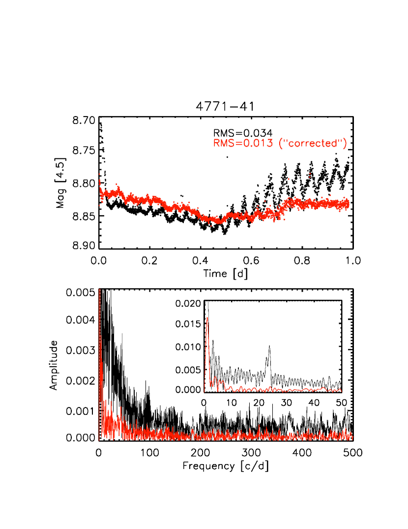
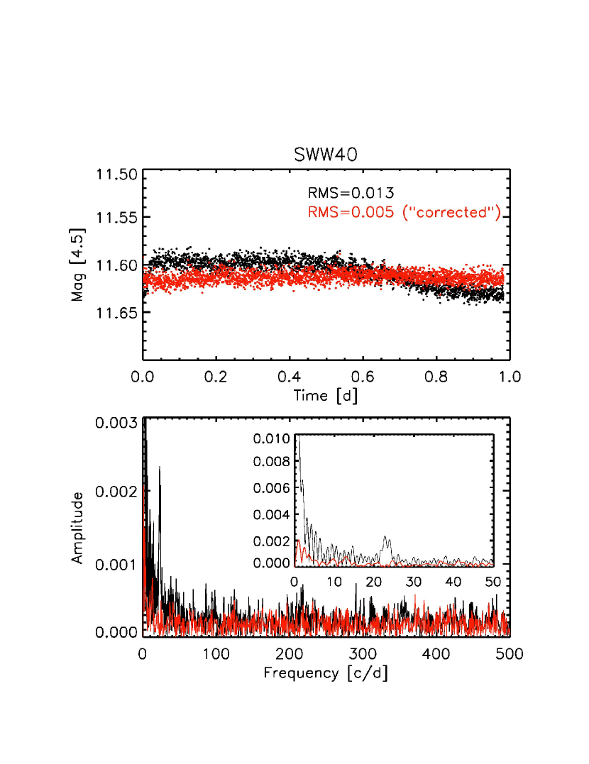
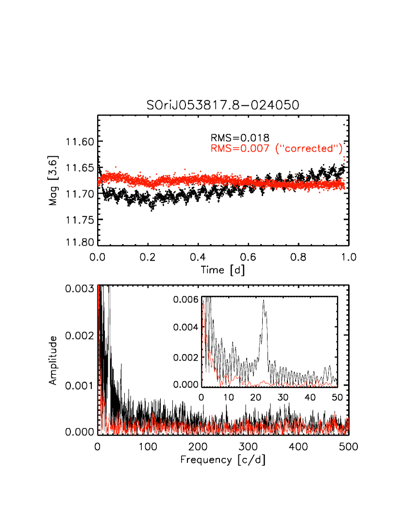
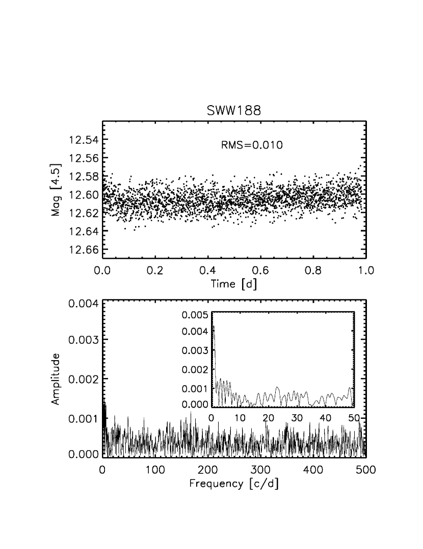
Figure 5.— Light curves and periodograms for all targets, in order of decreasing optical brightness. Object identifications are listed above each light curve, and the Spitzer band (3.6 or 4.5 $\mu$m) is noted in the y-axis label. Black indicates the raw light curve and periodogram, whereas red shows them after correction for intra-pixel sensitivity effects. Objects with no red points did not require correction. Periodogram frequencies are given in cycles per day. Insets show the same periodograms zoomed in to the low-frequency range where the signature of the pixel-phase oscillation is visible ($\sim$22-24 cd^-1).

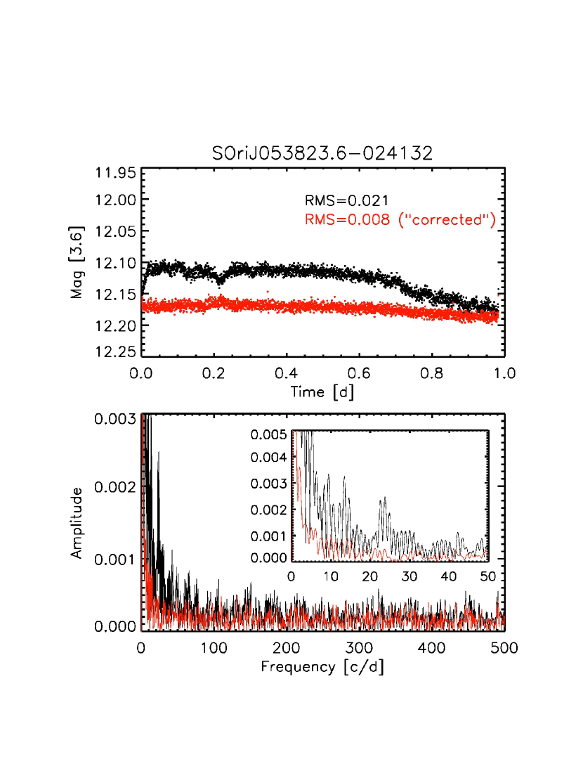
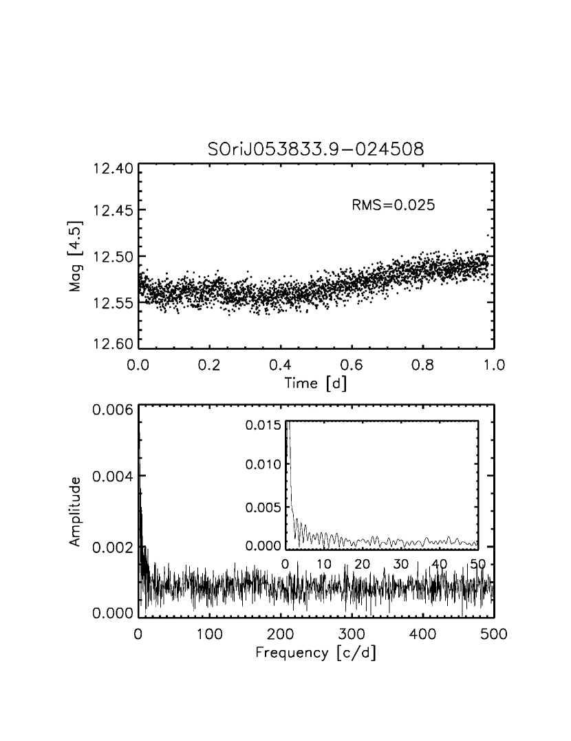
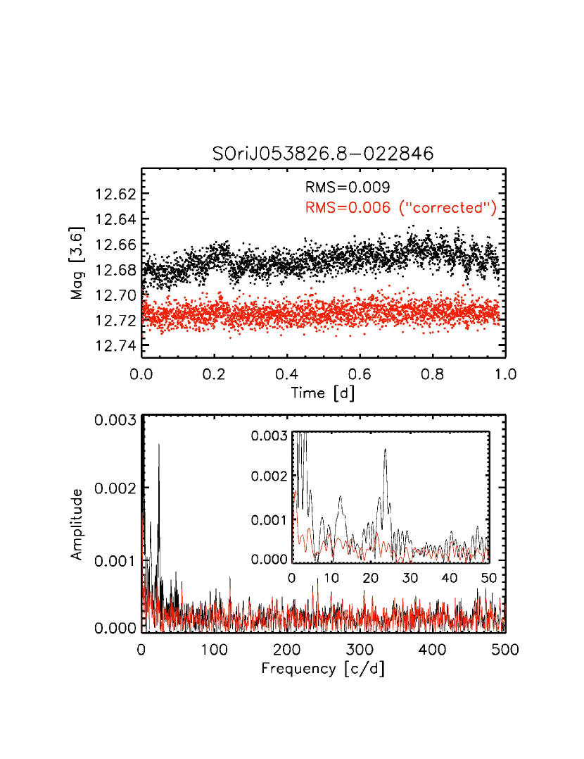
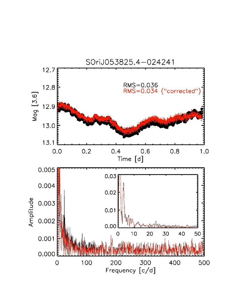
Figure 5.— (cont.)

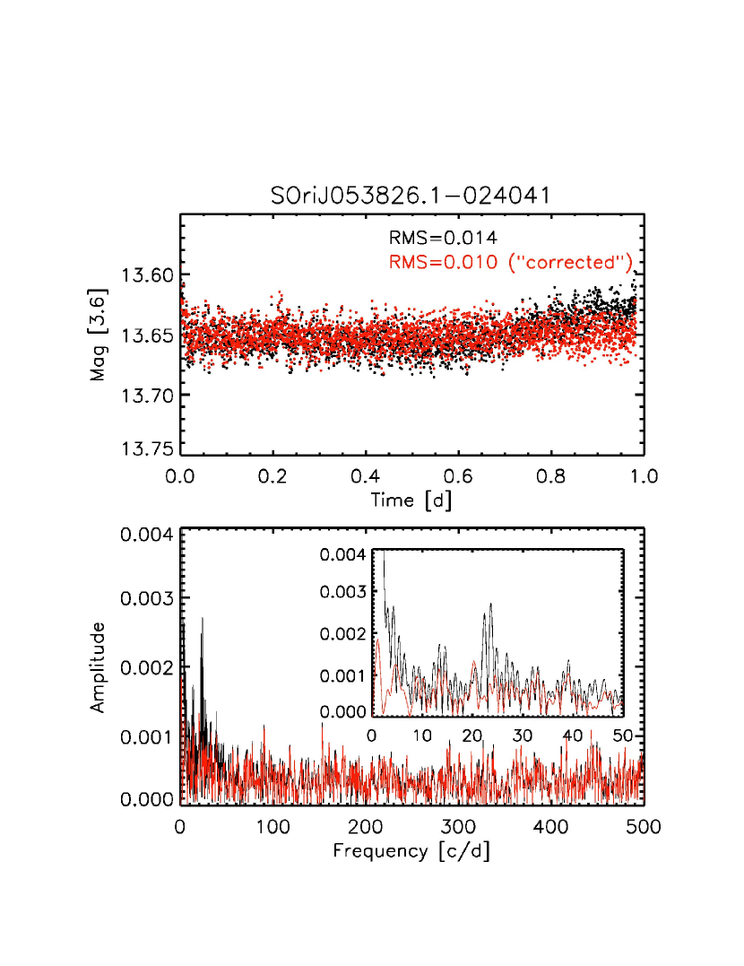
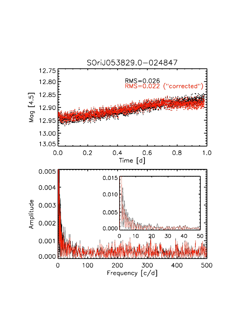
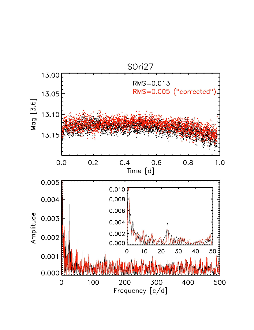
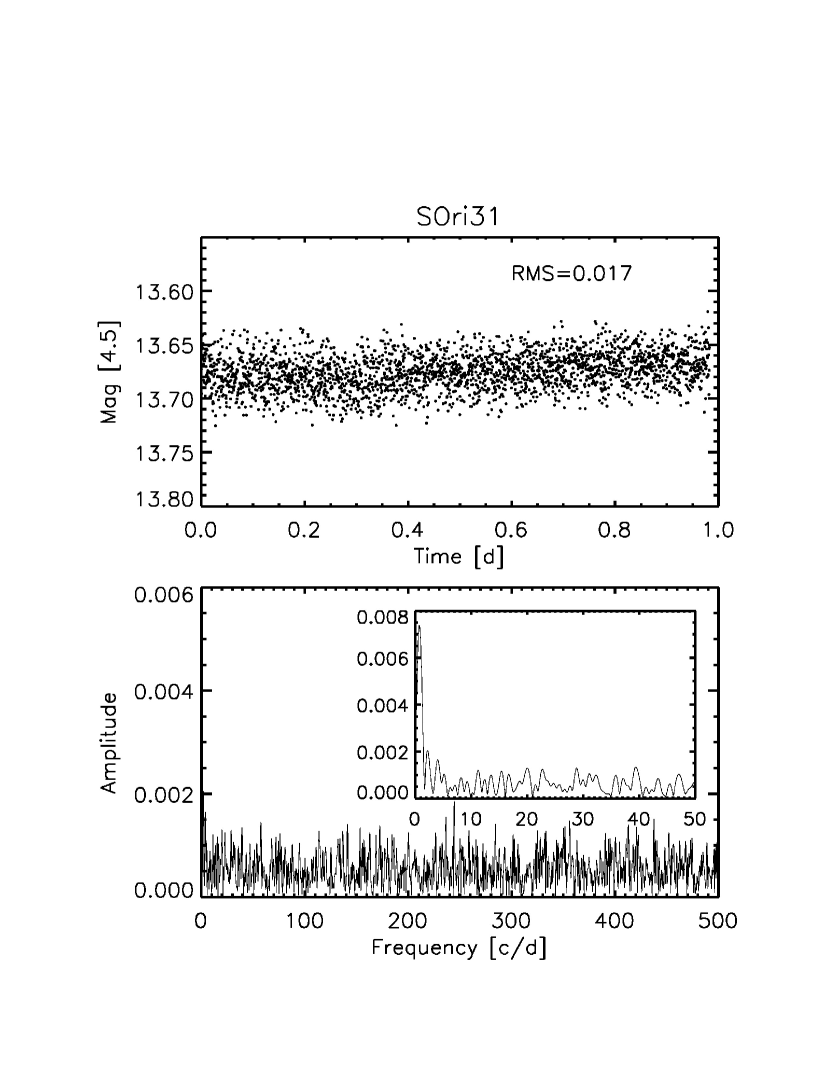
Figure 5.— (cont.)

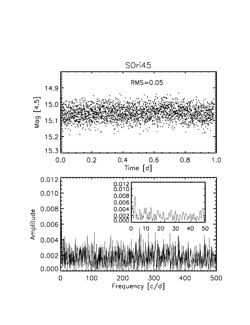
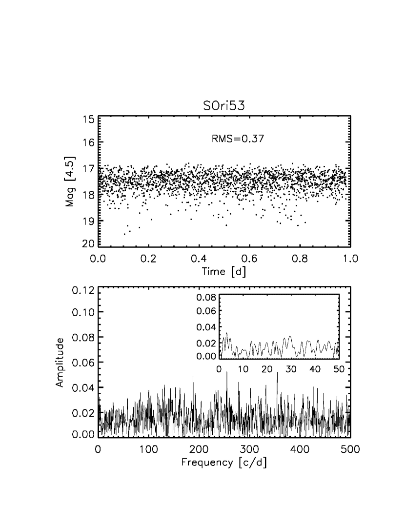
Figure 5.— (cont.)

Examination of the periodograms revealed that the pixel-phase correction process substantially lowered the noise level, enabling better sensitivity to periodicities outside the 1–1.1-hour range of the pixel-phase oscillation. The two exceptions were SOri 27 and 4771-41. The former was centered near the edge of two pixels, making a fit to the spatial distributions difficult without resorting to a more complex non-gaussian function. Object 4771-41 is exceedingly bright, and residual variability seen in the final light curve may be a figment of the correction process.

The majority of periodograms are relatively featureless, reflecting minimal variability in the input light curves. In the low-frequency region from one to several cd^-1, many of the periodograms steadily rise in a “1/$f$” fashion indicative of systematic or “red” noise trends (e.g., Press et al. 1992) close to the maximum timescale of one day. However, apart from one object (SOri J053825.4-024241), no potential periodic signals stand out high enough above the baseline. Here we have used a criterion of 4-$\sigma$, equivalent to 99.9% certainty, as explained in CH10. Since SOri J053825.4-024241 displays intrinsic aperiodic variability at the 10% level, and the putative 3.5 cd^-1 (or $\sim$9.6h) signal barely exceeds the detection threshold at S/N$\sim$4, it is unclear as to whether this is a true periodicity.

5.1. Prospects for pulsation

The lack of periodic signals in the 1–4-hour range suggests that none of the $\sigma$ Ori cluster members in our sample exhibits deuterium-powered pulsation at a level above several millimagnitudes. However, the strength of this conclusion depends on the likelihood that one or more targets fall on the PB05’s predicted pulsation instability strip. If we assume a distance of 350 pc for the $\sigma$ Ori cluster, then all seven BDs in the sample (S Ori J053825.4-024241, S Ori J053826.1-024041, S Ori 31, S Ori J053829.0-024847, S Ori 53, S Ori 27) may be on the instability strip, to within the uncertainties. If we instead adopt a distance of 440 pc, then the VLMS S Ori J053826.8-022846 becomes an additional candidate, whereas the position of S Ori 45 falls slightly off the strip. Thus one would naively expect that a handful of our targets have temperatures and luminosities consistent with those required for pulsational instability. Nevertheless, the significant size of the measurement uncertainties compared with the width of the strip must be taken into account.

To estimate the chance that in fact none of our sample have H-R diagram positions overlapping the instability strip, we adopt temperature-luminosity probability distributions for each object. We take the distributions to be two-dimensional asymmetric gaussians, normalized and centered at the adopted luminosities and temperatures. The gaussian widths are given by the associated 1-$\sigma$ uncertainties. The position of each target then corresponds to a probability that it is susceptible to pulsation, which we determine by integrating its distribution over the entire region of the instability strip. For objects on or very close to the strip, this value is $\sim$20-25%, whereas for the higher mass stars far from the strip it is close to zero. The probability that the position of a given object does not overlap with the instability strip then ranges from 75% to 100%. The product of these values over all targets provides an estimate of the chance that no pulsators would be present in our sample. For luminosities derived from $J$-band magnitudes and a cluster distance of 440 pc, this probability is 19%– small but certainly not negligible. Since systematic errors can significantly affect the result, we have also recalculated this value using both $I$-band-derived luminosities and the alternate distance of 350 pc. The different combinations yield probabilities from 23% to 32%. Turning these numbers around, there is a $\sim$70-80% chance that at least one object should exhibit pulsation based on its position within the instability strip, assuming that the theoretical calculations underpinning it (PB05) do not suffer from gross systematic errors.

In addition, the expectation value for the number of objects lying directly on the strip lies between one and two, depending on the choice of distance and $J$ or $I$ band magnitudes. Therefore if pulsation is operating at an observable level, we are likely to detect at least one instance of it. The fact that we also did not detect short-timescale variability in our larger ground-based sample (CH10) of BDs and VLMSs suggests that the lack of observable pulsation is a repeatable result and not the product of sample selection effects. Nevertheless, we caution that the small number of low-mass objects observed here leaves open the possibility that no true pulsation candidates were among our sample.

Assuming this is not the case, statistically we expect at least one object in our sample to be susceptible to pulsation. If so, the amplitude of this phenomenon appears to be too low to be observed in the infrared. To quantify the detection limit, we have fit power laws to each periodogram, tracing out the maximum amplitude level as a function of frequency. These curves, of form $A/(f+B)+C$ for frequency $f$ and constants $A$, $B$, and $C$, mark the highest amplitude signal observed for each object, whether real or noise. We display them in Fig. 6, where the procedure has been carried out on both the raw and pixel-phased corrected data.

Figure 6.— Limits on pulsation detection in the periodograms based on raw light curves. Solid red curves show the limits for objects on or near the instability strip, whereas grey dashed curves are for objects not expected to exhibit pulsation. The curve for S Ori 53 is off the chart at a uniform amplitude of 0.04 magnitudes. The dotted lines indicate the region of frequency space where we expect pulsation to occur (i.e., 1–4-hour periods). The left panel displays data before pixel-phase correction, and the right shows the final data after removal of pixel-phase oscillation trends. For the few objects that did not require these corrections, the curves derived directly from raw data are repeated.

For the majority of objects, we have detected no periodicities in the pulsation frequency range with amplitudes greater than several millimagnitudes. Brown dwarfs S Ori 45 and S Ori 53 are exceptions, as they have higher limits (0.005 and 0.04 magnitudes respectively in the 4.5 $\mu$m band) owing to their faintness and correspondingly high noise levels in both the light curves and periodograms. In addition, brown dwarf S Ori J053825.4-024241 has a higher limit for pulsation (0.004-0.007 magnitudes in the 3.6 $\mu$m band, depending on frequency) since it displays substantial intrinsic variability. The rest of our targets have maximum amplitudes in the periodogram of at most 0.002 to 0.003 magnitudes. This represents the threshold above which we detect no periodicities. We conclude that if deuterium-burning pulsation is present in any of our sources (apart from the three exceptions noted above), then its amplitude must be below this level.

5.2. SOriJ053825.4-024241: a high-amplitude variable brown dwarf

Among our sample, the substellar $\sigma$ Ori member SOriJ053825.4-024241 stands out as the lone target highly variable on timescales less than 24 hours. With a 3.6 $\mu$m band RMS of 0.035 magnitudes, this object has a peak-to-peak amplitude of 0.15 magnitudes. It displays variations about four times as large in the $I$-band, based on our longer timescale ground-based dataset (CH10). Other studies (Caballero et al. 2006) have indicated that SOriJ053825.4-024241 is actively accreting and has a disk (Hernández et al. 2007).

No previous infrared studies of brown dwarfs have uncovered aperiodic variability on such short timescales. However, variability of young stars at Spitzer wavelengths or of brown dwarfs in general with these amplitudes and on longer time scales is not unprecedented. The Young Stellar Object Variability (YSOVAR) project (Morales-Calderón 2011) campaign on young Orion Nebula Cluster stars (masses $\gtrsim$0.1 $M_{\odot}$) has also found substantial erratic variability in the 3.6 and 4.5 $\mu$m bands. Assessment of their data has shown that the aperiodic variables among the sample known to harbor disks display a range of variability RMS values centered on $\sim$0.03 magnitudes in the 3.6 $\mu$m band (Morales-Calderón 2011, private communication). Similar amplitude distributions were obtained using existing multi-epoch data with limited cadence in Taurus and Chamaeleon I by Luhman et al. (2008) and Luhman et al. (2010). The typical RMS of a few hundredths of a magnitude is quite consistent with the value that we have measured for S Ori J053825.4-024241. Morales-Calderón (2011) discuss the possible causes of the mid-infrared variability and surmise that many of their variables may be explained by variable obscuration by overdense regions in the inner disk, while others are caused by intrinsic changes in the inner disk emission itself. Either of these scenarios may apply to SOriJ053825.4-024241. In any case, hot accretion gas is likely too faint at infrared wavelengths to serve as the source of variability for this object.

To further explore the behavior of this BD on different timescales, we have performed an autocorrelation analysis. In addition to displaying quasi-periodicity patterns not picked up by the periodogram, it is useful in assessing the timescale on which the variability mechanism remains coherent. We have calculated an autocorrelation function based on the S Ori J053825.4-024241 light curve using both a standard, “biased” formula, as well as one that corrects for the finite data length. The standard autocorrelation function (ACF) is given by:

$$A(t)=\frac{1}{A(0)}\sum_{j=1}^{N-t/\Delta t}L(j)L(j+t/\Delta t),$$

where $L(j)$ are the light curve points, $\Delta t$ is the time spacing between datapoints (which must be uniform), $N$ is the total number of points, and the $A(0)$ factor in front in included so that at a time lag of zero, the ACF is completely correlated ($A(0)=1$).

To account for the fact that fewer points are available to calculate the ACF at longer lag times ($t>0.5$), we have produced another version- the “unbiased” ACF- in which the this roughly linear effect ($\sim N-t/\Delta t$)) has been divided out. In both cases, we have computed the autocorrelation via fourier transform of the power spectrum (as specified by the Wiener-Khinchin theorem; Wiener 1930, Khinchin 1934), since this is both faster and less prone to numerical inaccuracies.

Both versions of the ACF are plotted in Fig. 7. We find that the light curve is well correlated up to timescales of $\sim$0.15d, or 3.6h. At longer timescales, it also shows significant correlation due to the overall trend seen in the light curve; this is illustrated by the two peaks at $\sim$0.43d and $\sim$0.9d (the latter primarily in the unbiased ACF). We conclude that the variability mechanism is physically coherent on timescales of at least a few hours. The hypothesis of variable obscuration in association with the disk is qualitatively consistent if the scale of clumpiness and location of dust is such that fluctuations would pass by the face of the BD in several hours.

Figure 7.— Autocorrelation functions for SOriJ053825.4-024241. The solid line is the standard ACF, whereas the dashed line is the version that has been corrected for finite data length.

6. Comparison with optical data

Previously we observed a region including both Spitzer fields, using the CTIO 1.0-meter telescope (CH10). High cadence (every 10 minutes) data in the Cousins $I$ band and lower cadence (twice per night) data in $R$ was acquired over runs of 12 and 11 consecutive nights, respectively in 2007 and 2008. We identified a number of variable objects, both in the $\sigma$ Ori cluster and background field. Although the overall time baseline of the Spitzer observations is short compared to that of the ground-based campaign, we have searched for common variability in the two datasets.

A total of seven variable $\sigma$ Ori cluster members from the ground-based campaign fall in the fields of the Spitzer observations, as noted in Table 1. In the 4.5 $\mu$m field, S Ori J053833.9-024508 and 4771-41 were identified as aperiodic variables in the ground-based photometry. In addition, the BD S Ori 45 was identified as being periodic in the $I$-band, with a period of 7.2 hours and amplitude 0.034 magnitudes, whereas VLMS SWW40 was found to have a period of 4.47 days and amplitude 0.013 magnitudes. In the 3.6 $\mu$m field, the BD S Ori J053825.4-024241 was identified as an aperiodic variable, as discussed in $\S$5.2. Two additional variables were found be periodic in the $I$ band: S Ori J053823.6 ($P$=1.7d; $A$=0.017 mags) and S Ori J053817.8-024050 ($P$=2.4d; $A$=0.008 mags).

For those ground-based variables with brightness fluctuations on timescales longer than a day, we do not necessarily expect to observe variability in our shorter Spitzer dataset. Indeed, we do not recover periodic variability at great than the 1% level in any of the ground-based periodic variables. In addition to the shorter time baseline, it is possible that the non-simultaneity of observations and the different wavelengths make rotational spot modulation– the primary explanation for periodic variability in young VLMSs and BDs– unobservable in our light curves.

Several of the previously identified aperiodic variables, on the other hand, do appear to be variable at infrared wavelengths. The BD S Ori J053825.4-024241 displays relatively high amplitude erratic fluctuations (see $\S$5.2). Object 4771-41 shows residual variability after correction for the pixel-phase effect (light curve RMS of $\sim$0.01 versus $\sim$0.001 magnitudes), and S Ori J053833.9-024508 also displays variability at a significantly higher level than predicted by signal-to-noise estimates (light curve RMS of $\sim$0.05 versus $<$0.01 magnitudes). The RMS values in the Spitzer bands are similar to those found in the optical for S Ori J053825.4-024241 and S Ori J053833.9-024508, whereas they are roughly an order of magnitude lower for 4771-41. Thus the light curve of this latter object may exhibit residual pixel-phase effects, as opposed to real variability. However, for the other two aperiodic variables, the rough correspondence of RMS amplitudes in both the optical and infrared suggests that the variability mechanism may be relatively insensitive to wavelength.

Interestingly, object S Ori J053829.0-024847 displays substantial variability at 4.5 $\mu$m (an 0.06-magnitude drift over 24 hours), whereas it did not appear variable in our ground-based dataset. We suspect that the variability mechanism in this case was dormant during the optical observations, although its photometry could have been affected by a nearby neighbor on the array. Since this object exhibits an infrared excess (Hernández et al. 2007, Caballero et al. 2007), there is an additional possibility that the variability is associated with the disk and thus only visible in the near-infrared and at longer wavelengths.

In addition to the recovery of aperiodic variability in our $\sigma$ Ori cluster sample, we also re-identify a number of eclipsing binaries; further details on these field objects are provided in the appendix.

7. Conclusions

We have presented high-cadence infrared light curves of 14 low-mass $\sigma$ Orionis cluster members based on Warm Spitzer observations. The excellent precision of our photometry led to limits of 0.002–0.003 magnitudes on the amplitude of any deuterium-burning pulsation in these objects in the 3.6 and 4.5 $\mu$m bands. This result is consistent with our ground-based $I$-band findings, which revealed no periodicities with amplitudes greater than 0.01 magnitudes and timescales shorter than 7 hours among low-mass $\sigma$ Ori cluster members. In this work we have reduced the amplitude limit by an order of magnitude, albeit on a smaller sample of BDs and VLMSs. Notably, we also find little other variability on the $<$24-hour timescales probed by the data. The main exception was brown dwarf S Ori J053825.4-024241, which displays brightness variations of up to 0.1 magnitudes over the course of a day. The similarity of amplitudes in the infrared and optical suggests that obscuration by dust material in the surrounding disk provides a better explanation than does variable light scattering or accretion (e.g., van Boekel et al. 2010). We propose that a general lack of variability among young, low-mass cluster members may in fact be useful for future studies at infrared wavelengths, such as searches for planets around young BDs and VLMSs. Both transit detection and radial velocity measurements benefit from low levels of spot-related activity on short timescales.

We also emphasize that production of light curves devoid of the pixel-phase and other detector effects is difficult at present with Warm Spitzer data. While previous work has successfully identified low-amplitude planetary transit signatures in Spitzer light curves (e.g., Deming et al. 2011), the transit event represents only a small portion of these time series and hence systematic trends can be taken into account. When the entire light curve is instead the subject of interest, and the form of variability is unknown in advance, systematics are more difficult to model and remove. For future high-precision photometric time series work, we recommend further exploration of the sensitivity distribution within individual pixels, perhaps through even higher cadences that might provide more datapoints over a given time and thus greater spatial coverage within individual pixels.

Appendix

In addition to examining the light curves of the 14 $\sigma$ Ori cluster member targets, we also searched the entire 3.6 and 4.5 $\mu$m fields for serendipitous foreground and background variables. After producing light curves for all point sources with magnitudes less than $\sim 19.0$, we assessed their RMS spread as a function of brightness. Objects lying more than three standard deviations above the median trend were flagged as possible variables. We visually examined their light curves and disregarded those whose brightness fluctuations were clearly caused by pixel sensitivity effects. Four objects (other than BD 053825.4-024241; $\S$5.2) displayed conspicuous variability by these criteria; their light curves are presented in Fig. 8. For consistency with the other presented light curves, we show both the time series and their periodograms. We list the estimated period, which often does not correspond to the largest periodogram peak since this analysis method is relatively insensitive to the presence of secondary eclipses.

All four stars were also identified as variables in our $I$-band ground-based dataset (CH10); therefore, we refer to them by the same nomenclature. We have not rigorously fit eclipse profiles or other models to the data but present estimates ($\sim$10–20% accuracy) of their main parameters here:

CTIO J05381870-0246582 is an eclipsing binary system with an $I$-band depth of $\sim$0.45 magnitudes, and 4.5 $\mu$m depth of at least 1.2 magnitudes. The most likely period is $\sim$11.8 hours, or 5.9 hours if all of the eclipses are primary (the data are too noisy to to distinguish different depths in subsequent eclipses).

CTIO J05382129-0240318 also appears to be an eclipsing binary, with period $\sim$9.6 hours. This period is fully consistent with our ground-based data, for which we unfortunately reported an erroneous value (4.6 days instead of 9.5 hours). The 3.6 $\mu$m depth ($\gtrsim 1.3$ magnitudes) is significantly deeper than the $I$-band depth ($\sim$0.35 magnitudes).

2MASS J05382188-0241039 exhibits a slightly asymmetric periodic profile, reminiscent of an RR Lyrae star. Its period of 11.8h is also consistent with this type of pulsator. Since the timescale is so close to half a day, aliasing caused us to misidentify and report a 1.0d period for the ground-based data. The 3.6 $\mu$m peak-to-peak amplitude is $\sim$0.25 magnitudes, whereas the value at $I$ band is just over 0.6 magnitudes.

2MASS J05381949-0241224 also displays the characteristic shape of a close eclipsing binary, although there is slight decrease in its peak amplitude over 24 hours which may be attributed to systematic pixel sensitivity effects. The period is 2.8 or 5.6 hours, depending on whether alternating brightness dips are secondary eclipses. At $\sim$0.5 magnitudes, the peak-to-peak amplitude at 3.6 $\mu$m is about 20% smaller than that in the $I$ band.

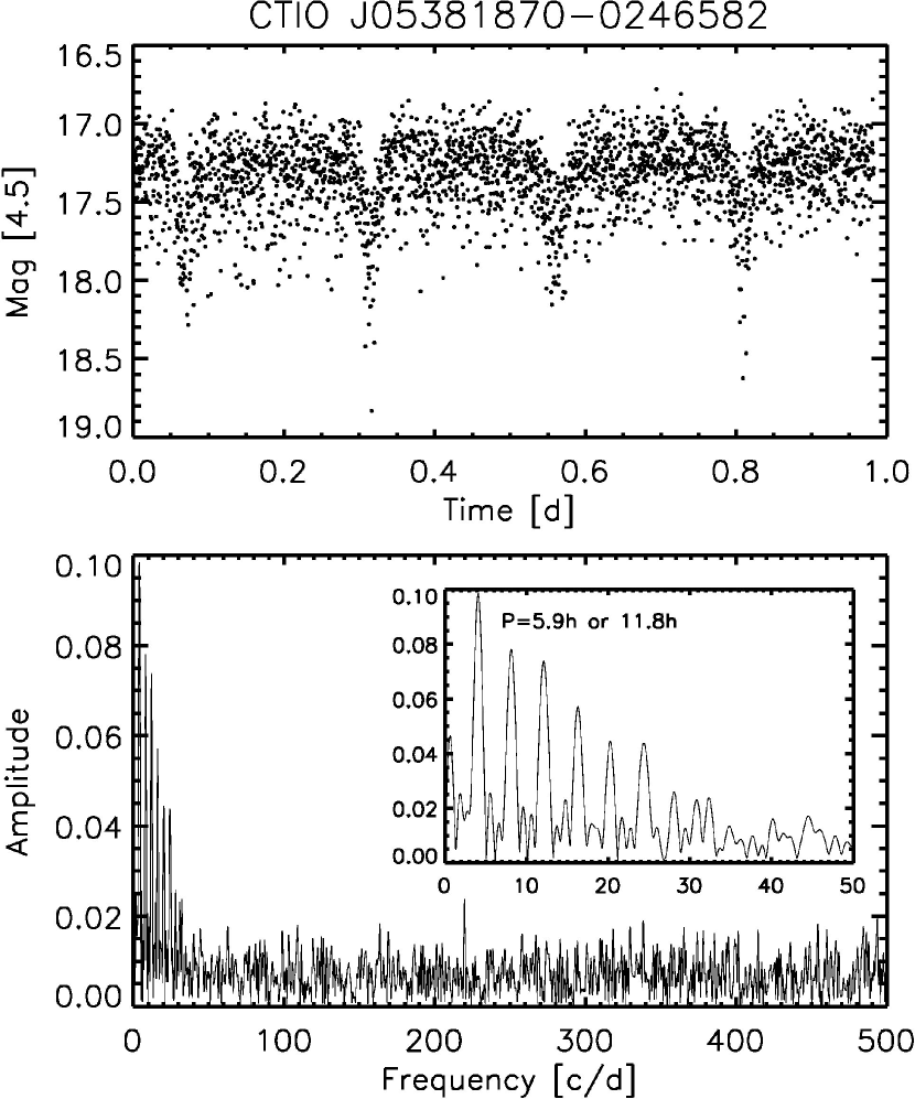
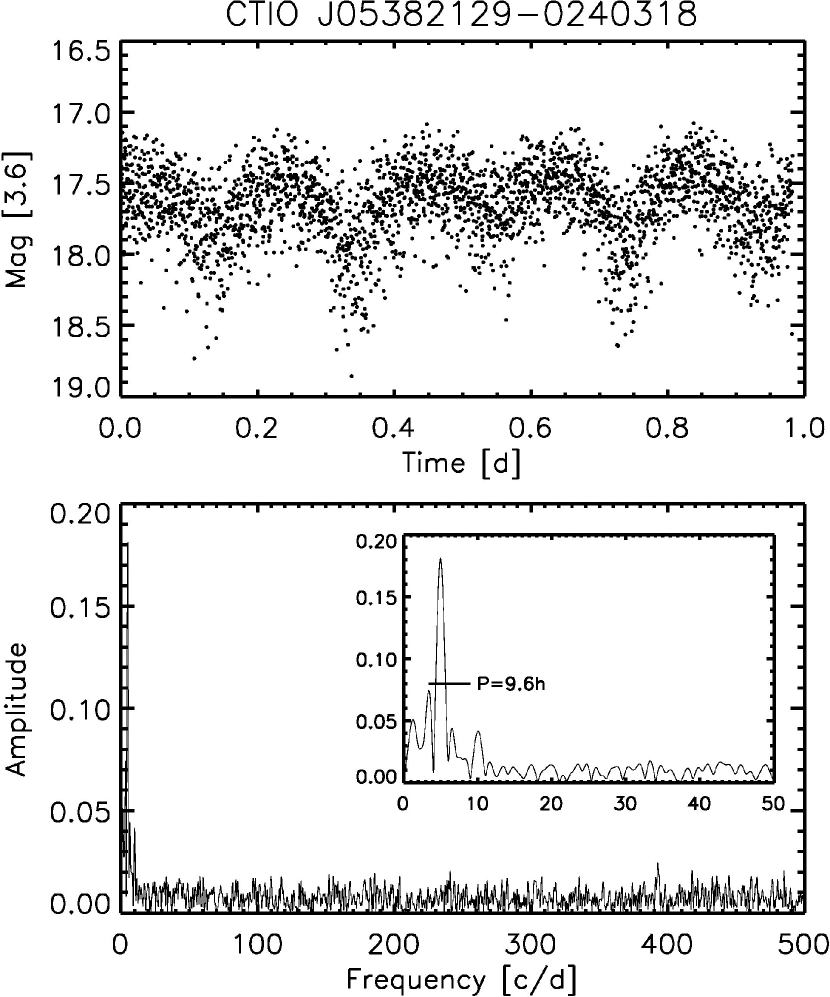
Figure 8.— Field variable stars. Light curves (top) and periodograms (bottom) are as in Fig. 5; estimated periods are marked near the corresponding frequency peaks.

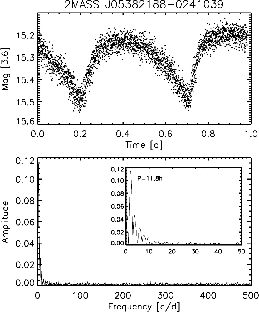
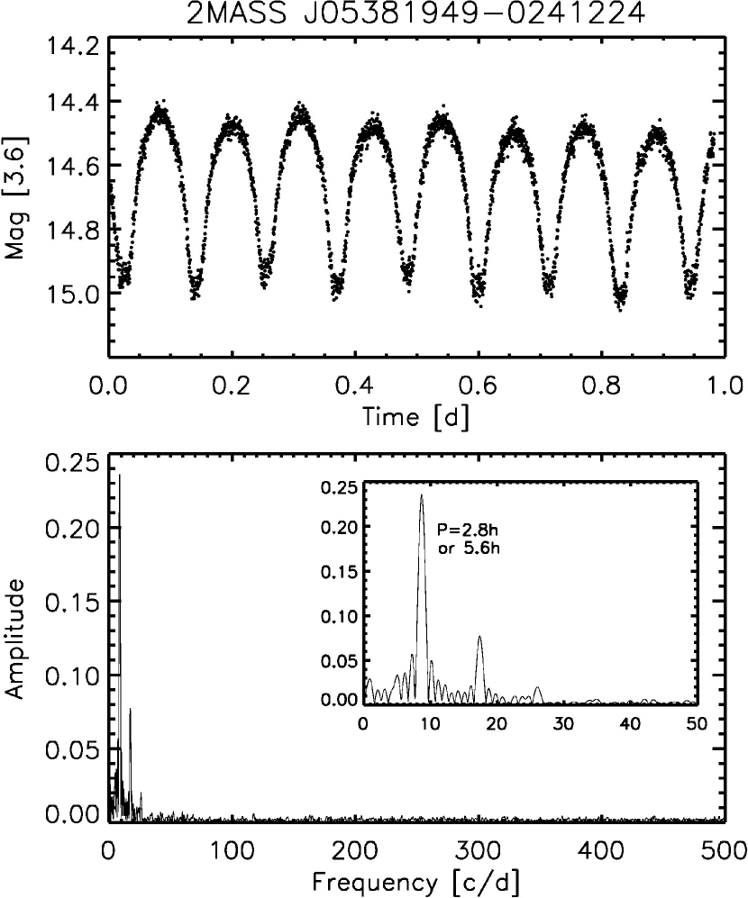
Figure 8.— (cont.)

References

- Bailer-Jones & Mundt (2001) Bailer-Jones, C. A. L., & Mundt, R. 2001, A&A, 367, 218
- Ballard et al. (2010) Ballard, S., Charbonneau, D., Deming, D., Knutson, H. A., Christiansen, J. L., Holman, M. J., Fabrycky, D., Seager, S., & A’Hearn, M. F. 2010, PASP, 122, 1341
- Baraffe et al. (1998) Baraffe, I., Chabrier, G., Allard, F., & Hauschildt, P. H. 1998, A&A, 337, 403
- Baraffe et al. (2003) Baraffe, I., Chabrier, G., Barman, T. S., Allard, F., & Hauschildt, P. H. 2003, A&A, 402, 701
- Barrado y Navascués et al. (2003) Barrado y Navascués, D., Béjar, V. J. S., Mundt, R., Martín, E. L., Rebolo, R., Zapatero Osorio, M. R., & Bailer-Jones, C. A. L. 2003, A&A, 404, 171
- Barrado y Navascués et al. (2001) Barrado y Navascués, D., Zapatero Osorio, M. R., Béjar, V. J. S., Rebolo, R., Martín, E. L., Mundt, R., & Bailer-Jones, C. A. L. 2001, A&A, 377, L9
- Béjar et al. (1999) Béjar, V. J. S., Zapatero Osorio, M. R., & Rebolo, R. 1999, ApJ, 521, 671
- Caballero (2008) Caballero, J. A. 2008, A&A, 478, 667
- Caballero et al. (2007) Caballero, J. A., Béjar, V. J. S., Rebolo, R., Eislöffel, J., Zapatero Osorio, M. R., Mundt, R., Barrado Y Navascués, D., Bihain, G., Bailer-Jones, C. A. L., Forveille, T., & Martín, E. L. 2007, A&A, 470, 903
- Caballero et al. (2006) Caballero, J. A., Martín, E. L., Zapatero Osorio, M. R., Béjar, V. J. S., Rebolo, R., Pavlenko, Y., & Wainscoat, R. 2006, A&A, 445, 143
- Cody & Hillenbrand (2010) Cody, A. M., & Hillenbrand, L. A. 2010, ApJS, 191, 389
- Deeming (1975) Deeming, T. J. 1975, Ap&SS, 36, 137
- Deming et al. (2011) Deming, D., Knutson, H., Agol, E., Desert, J., Burrows, A., Fortney, J. J., Charbonneau, D., Cowan, N. B., Laughlin, G., Langton, J., Showman, A. P., & Lewis, N. K. 2011, ApJ, 726, 95
- Fazio (2004) Fazio, G. G. e. a. 2004, ApJS, 154, 10
- Frasca et al. (2009) Frasca, A., Covino, E., Spezzi, L., Alcalá, J. M., Marilli, E., Fżrész, G., & Gandolfi, D. 2009, A&A, 508, 1313
- Hernández et al. (2007) Hernández, J., Hartmann, L., Megeath, T., Gutermuth, R., Muzerolle, J., Calvet, N., Vivas, A. K., Briceño, C., Allen, L., Stauffer, J., Young, E., & Fazio, G. 2007, ApJ, 662, 1067
- Jeffries et al. (2006) Jeffries, R. D., Maxted, P. F. L., Oliveira, J. M., & Naylor, T. 2006, MNRAS, 371, L6
- Khinchin (1934) Khinchin, A. Y. 1934, Mathematische Annelen, 109, 604
- Koldoba et al. (2008) Koldoba, A. V., Ustyugova, G. V., Romanova, M. M., & Lovelace, R. V. E. 2008, MNRAS, 388, 357
- Kraus & Hillenbrand (2007) Kraus, A. L., & Hillenbrand, L. A. 2007, AJ, 134, 2340
- Lodieu et al. (2009) Lodieu, N., Zapatero Osorio, M. R., Rebolo, R., Martín, E. L., & Hambly, N. C. 2009, A&A, 505, 1115
- Luhman (1999) Luhman, K. L. 1999, ApJ, 525, 466
- Luhman et al. (2008) Luhman, K. L., Allen, L. E., Allen, P. R., Gutermuth, R. A., Hartmann, L., Mamajek, E. E., Megeath, S. T., Myers, P. C., & Fazio, G. G. 2008, ApJ, 675, 1375
- Luhman et al. (2010) Luhman, K. L., Allen, P. R., Espaillat, C., Hartmann, L., & Calvet, N. 2010, ApJS, 186, 111
- Luhman et al. (2003) Luhman, K. L., Stauffer, J. R., Muench, A. A., Rieke, G. H., Lada, E. A., Bouvier, J., & Lada, C. J. 2003, ApJ, 593, 1093
- Morales-Calderón et al. (2006) Morales-Calderón, M., Stauffer, J. R., Kirkpatrick, J. D., Carey, S., Gelino, C. R., Barrado y Navascués, D., Rebull, L., Lowrance, P., Marley, M. S., Charbonneau, D., Patten, B. M., Megeath, S. T., & Buzasi, D. 2006, ApJ, 653, 1454
- Morales-Calderón (2011) Morales-Calderón, M. e. a. 2011, ApJ, 733, 50
- Orlando et al. (2010) Orlando, S., Sacco, G. G., Argiroffi, C., Reale, F., Peres, G., & Maggio, A. 2010, A&A, 510, A71+
- Palla & Baraffe (2005) Palla, F., & Baraffe, I. 2005, A&A, 432, L57
- Press et al. (1992) Press, W. H., Teukolsky, S. A., Vetterling, W. T., & Flannery, B. P. 1992, Numerical recipes: The art of scientific computing (Cambridge: Cambridge University Press)
- Scholz & Eislöffel (2004) Scholz, A., & Eislöffel, J. 2004, A&A, 419, 249
- Sherry et al. (2008) Sherry, W. H., Walter, F. M., Wolk, S. J., & Adams, N. R. 2008, AJ, 135, 1616
- Slesnick et al. (2006a) Slesnick, C. L., Carpenter, J. M., & Hillenbrand, L. A. 2006a, AJ, 131, 3016
- Slesnick et al. (2006b) Slesnick, C. L., Carpenter, J. M., Hillenbrand, L. A., & Mamajek, E. E. 2006b, AJ, 132, 2665
- van Boekel et al. (2010) van Boekel, R., Juhász, A., Henning, T., Köhler, R., Ratzka, T., Herbst, T., Bouwman, J., & Kley, W. 2010, A&A, 517, A16+
- Werner (2004) Werner, M. W. e. a. 2004, ApJS, 154, 1
- Wiener (1930) Wiener, N. 1930, Acta Mathematica, 55, 117
- Zapatero Osorio et al. (2003) Zapatero Osorio, M. R., Caballero, J. A., Béjar, V. J. S., & Rebolo, R. 2003, A&A, 408, 663