Distributed tracking control of leader-follower multi-agent systems under noisy measurement

Abstract

In this paper, a distributed tracking control scheme with distributed estimators has been developed for a leader-follower multi-agent system with measurement noises and directed interconnection topology. It is supposed that each follower can only measure relative positions of its neighbors in a noisy environment, including the relative position of the second-order active leader. A neighbor-based tracking protocol together with distributed estimators is designed based on a novel velocity decomposition technique. It is shown that the closed loop tracking control system is stochastically stable in mean square and the estimation errors converge to zero in mean square as well. A simulation example is finally given to illustrate the performance of the proposed control scheme.

[cor]Corresponding author: Jiangping Hu. Tel. +86-28-61831590. Fax +86-28-61831113.  and

1 Introduction

In recent years cooperative distributed control of multi-agent systems has been a research focus in control community. An important control strategy among many others is the leader-following coordination among a team of agents. The leader-follower approach has been widely used in many practical applications such as formation control in robotic systems (Wang P. K. C., (1991); Das,Fierro$,\&$Kumar, (2002)), unmanned aerial vehicle (UAV) formation (Vanek,Peni,et al., (2005); Anderson,Fidan,et al., (2008)), target tracking in sensor network (Gupta,Cao$,\&$Haering, (2008); Hu$,\&$Hu, (2008)), and so on.

The major issues addressed in the study of leader-follower multi-agent systems include the varieties of topological consensus conditions (Jadbabaie,Lin$,\&$Morse, (2003); Ren$,\&$Beard, (2005)), the roles of multiple leaders in guiding the followers (Lin,Francis$,\&$Maggiore, (2005); Shi$,\&$Hong, (2009)), the time-delayed control design (Hu$,\&$Hong, (2007); Lin,Jia, et al., (2008)), and the distributed estimation strategies (Fax$,\&$Murray, (2004); Hong,Hu$,\&$Gao, (2006)). A common feature of these existing works on distributed control for leader-follower multi-agent systems is that the measurement noises are not considered. However in practice,the measurements and information communication are always subject to noises and/or perturbations, such as sensor noise, channel fading, quantization errors, etc. More recently consensus control problems with measurement noises have been studied in Li$,\&$Zhang, (2009) and Huang$,\&$Manton, (2009) with the fixed and undirected network topology. Huang$,\&$Manton, (2009) proposed a consensus control for a leaderless multi-agent system with the first order discrete-time dynamics under noisy measurements and proved that the average consensus can be achieved in the sense of mean square by introducing a decreasing gain if the network topology is a strongly connected circulant graph. Li$,\&$Zhang, (2009) extended the result to the first order continuous-time average consensus problem and obtained a sufficient and necessary condition. To the best of our knowledge, there is no report in open literature on design of distributed control for a leader-follower multi-agent system with measurement noises and time-varying directed interconnection topology.

In this paper, we will consider a distributed control design for a leader-follower multi-agent system under partial and noisy measurements and time-varying directed network topology. A novel velocity decomposition technique, inspired by the stochastic approximation approach (Nevelson$,\&$Hasminskii, (1976)), and a distributed estimation algorithm for the velocity of the active leader have been proposed to deal with those partial and noisy measurements. It has been shown that the estimation is convergent in mean square and the resulting closed loop control system is stochastically stable in mean square.

The remainder of this paper is organized as follows. In Section 2, some concepts in algebraic graph theory are briefly reviewed and a leader-following problem is formulated. In Section 3, a tracking control along with a distributed estimation algorithm is firstly designed for the leader-follower multi-agent system based on the velocity decomposition technique. Then the stochastic stability of the closed-loop tracking error system is analyzed under switched directed topology. A numerical example is given to illustrate the distributed tracking control for the leader-follower multi-agent system in Section 4. Finally, some concluding remarks and future research directions are given in Section 5.

Throughout this paper, we will use the following notations. $I$ denotes an appropriate dimensioned identity matrix; $\mathbf{1}$ denotes a column vector with all ones. For a given matrix $A$, $A^{T}$ denotes its transpose; $tr(A)$ its trace; $\|A\|$ its Frobenius norm; $\lambda_{\rm max}(A)$ and $\lambda_{\rm min}(A)$ its maximum and minimum eigenvalues respectively. For a given set $S$, $\chi_{S}$ denotes the indicator function of $S$. $E[\cdot]$ is the expectation operator; $col(\cdot)$ denotes the concatenation. For any given real numbers $a$ and $b$, $a\wedge b$ denotes $min\{a,b\}$.

2 Problem formulation

2.1 Preliminaries

In order to describe the interconnection topology of a leader-follower multi-agent system, we need to introduce some preliminaries from algebraic graph theory Godsil$,\&$Royle, (2001).

Let $\mathcal{G}=(\mathcal{V},\mathcal{E})$ be a directed graph (or digraph for simplicity) consisting of a finite set of vertices $\mathcal{V}=\{0,1,...,n\}$ and a finite set of arcs $\mathcal{E}\subseteq\mathcal{V}\times\mathcal{V}$. The order of $\mathcal{G}$ is the number of vertices in $\mathcal{G}$ and denoted by $|\mathcal{G}|$. An arc of $\mathcal{G}$ is denoted by $(i,j)$, which starts from $i$ and ends on $j$ and represents the information flow from agent $j$ to agent $i$. A path in $\mathcal{G}$ is a sequence $i_{0},i_{1},\cdots,i_{q}$ of distinct vertices such that $(i_{j-1},i_{j})$ is an arc for $j=1,\cdots,q$. If there exists a path from vertex $i$ to vertex $j$, we say that vertex $j$ is reachable from vertex $i$. Furthermore, if there exists a path from every vertex to vertex $j$, then vertex $j$ is a globally reachable vertex of $\mathcal{G}$. A digraph $\mathcal{G}$ is strongly connected if there exists a path between any two distinct vertices. A digraph $\mathcal{G}^{f}$ is a subgraph of $\mathcal{G}$ if its vertex set $\mathcal{V}(\mathcal{G}^{f})\subseteq\mathcal{V}$, arc set $\mathcal{E}(\mathcal{G}^{f})\subseteq\mathcal{E}$ and every arc in $\mathcal{E}(\mathcal{G}^{f})$ has both end-vertices in $\mathcal{V}$. A subgraph $\mathcal{G}^{f}$ is an induced subgraph if two vertices of $\mathcal{G}^{f}$ are adjacent in $\mathcal{G}^{f}$ if and only if they are adjacent in $\mathcal{G}$. An induced subgraph $\mathcal{G}^{f}$ that is strongly connected and maximal (i.e., no more vertices can be added while preserving its connectedness) is called a strong component of $\mathcal{G}$. In this paper we will use the vertex set $\mathcal{V}(\mathcal{G}^{f})=\{1,\cdots,n\}$ of subgraph $\mathcal{G}^{f}$ to label the follower-agents. For a vertex $i$ of $\mathcal{G}^{f}$, we call $\mathcal{N}_{i}=\{j:(i,j)\in\mathcal{E}\}$ the neighbor set of vertex $i$. A nonnegative matrix $A=[a_{ij}]\in\mathbf{R}^{n\times n}$ is called an adjacency matrix of subgraph $\mathcal{G}^{f}$ if the element $a_{ij}$ associated with the arc $(i,j)$ is positive, i.e. $a_{ij}=1\Leftrightarrow(i,j)\in\mathcal{E}$. Moreover, we assume $a_{ii}=0$ for all $i\in\mathcal{V}$. Notice that the adjacency matrix $A$ may not be a symmetric matrix for a digraph. If $\sum\limits_{j=1}^{n}a_{ij}=\sum\limits_{j=1}^{n}a_{ji}$ for $i=1,\cdots,n,$ then the digraph $\mathcal{G}^{f}$ is called balanced. A diagonal matrix $D=diag\{d_{1},...,d_{n}\}\in\mathbf{R}^{n\times n}$ is called the degree matrix whose diagonal elements $d_{i}=\sum\limits_{j=1}^{n}a_{ij}$ for $i=1,...,n$. Then the Laplacian matrix of subgraph $\mathcal{G}^{f}$ is defined as

$$L=D-A,$$ (1)

which may not be a symmetric matrix either. By this definition every row sum of the Laplacian matrix $L$ is zero. Therefore, $L$ always has a zero eigenvalue corresponding to a right eigenvector $\textbf{1}=col(1,\cdots,1)\in\mathbf{R}^{n}$. Moreover, if subgraph $\mathcal{G}^{f}$ is balanced, $L$ has a zero eigenvalue corresponding to a left eigenvector $\textbf{1}\in\mathbf{R}^{n}$.

When the digraph $\mathcal{G}$ is used to describe the interconnection topology of a multi-agent system consisting of one active leader-agent and $n$ follower-agents, we can define a diagonal matrix $B=diag\{a_{10},\cdots,a_{n0}\}\in\mathbf{R}^{n}$ to be a leader adjacency matrix, where $a_{i0}=1$ if follower $i$ is connected to the leader across the communication link $(i,0)$, otherwise, $a_{i0}=0$.

If we define a new matrix $H=L+B\in\mathbf{R}^{n},$ the following lemma plays a key role in sequel.

Lemma 1.

(Hu$,\&$Hong, (2007)) The following statements are equivalent:

1. Vertex $0$ is a globally reachable vertex of digraph $\mathcal{G}$;

2. $H$ is a positive stable matrix whose eigenvalues have positive real-parts;

3. Furthermore, if $\mathcal{G}^{f}$ is balanced, $H+H^{T}$ is a symmetric positive definite matrix.

Remark 2.

The topology connectedness in the sense that vertex $0$ is a globally reachable vertex of digraph $\mathcal{G}$ implies that the information of the leader can be propagated over the multi-agent network. Obviously, this notion of connectedness is much weaker than the notion of strong connectedness.

For the purpose of modelling the time-variation of the interconnection topology $\mathcal{G}$ of the leader-follower multi-agent system, we adopt the following general assumptions:

• There exists a switching signal $\sigma:[t_{0},\infty)\rightarrow\mathcal{P}=\{1,2,\cdots,N\}$, which is piecewise-constant. Here, $N$ denotes the total number of all possible interconnection topologies of the multi-agent system and $t_{0}$ is the initial time.

• If the time interval $[t_{0},\infty)$ is constituted by an infinite sequence of bounded, non-overlapping, contiguous time-intervals $[t_{j},t_{j+1})$ for $j=0,1,\cdots$ with $t_{0}=0$, there exists a positive constant $\tau$ such that $t_{j+1}-t_{j}\geq\tau$. The number $\tau$ is called a dwell time.

Then during each time-interval $[t_{j},t_{j+1})$ the digraph $\mathcal{G}_{\sigma(t)}$ is time-invariant and denoted by $\mathcal{G}_{p}$ for some $p\in\mathcal{P}$.

2.2 Leader-following problem

In this paper we will study a distributed control design for a leader-follower multi-agent system with one active leader-agent (just called leader in sequel for simplicity and labeled 0) and $n$ cooperative follower-agents (just called followers in sequel for simplicity). Consider a tracking control problem for a multi-agent system where the followers are moving with the first-order dynamics

$$\dot{x}_{i}(t)=u_{i}(t),$$ (2)

for $i=1,\cdots,n$, and the dynamics of the leader is described by the second-order differential equation

$$\begin{cases}\dot{x}_{0}(t)=v_{0}(t),\\ \dot{v}_{0}(t)=a_{0}(t),\\ y_{0}(t)=x_{0}(t).\end{cases}$$ (3)

The variables $x_{i}(t),u_{i}(t)\in\mathbf{R}^{m}\;(i=1,\cdots,n)$ denote the states and inputs of $n$ followers respectively while $x_{0}(t),v_{0}(t)\in\mathbf{R}^{m}$ and $a_{0}(t)\in\mathbf{R}^{m}$ denote the position, the velocity and the acceleration of the the active leader respectively, and $y_{0}(t)$ is the only output. Here for notation simplicity let $m=1$.

It was assumed in most existing works that an information exchange between agents is perfect, that is, each agent can obtain the information of its neighbors precisely. In addition, it was assumed that the interconnection topology of the followers are undirected. However, these assumptions are not valid in most practical situations due to various reasons, such as sensor and/or communication constraints, link variations. Measurement noises and time-varying directed graph have to be considered for control of leader-follower multi-agent systems.

Since the velocity $v_{0}(t)$ of the active leader cannot be measured by followers, then each follower has to make estimation of $v_{0}(t)$ for control design by using the noisy measurements from its neighbors. Our objective is to design a distributed control for the leader-follower multi-agent system under partial and noisy measurements and time-varying directed interconnection topology so that each follower can track the active leader and the velocity estimation errors are convergent to zero in the sense of mean square, i.e.,

$$\lim\limits_{t\to\infty}E[(x_{i}(t)-x_{0}(t))^{2}] =0,$$ (4)

$$\lim\limits_{t\to\infty}E[(v_{i}(t)-v_{0}(t))^{2}] =0,$$

where $v_{i}(t)$ is the estimate of $v_{0}(t)$ for the $i$th follower. In this case, the closed loop system is said to be stochastically stable in mean square.

3 Distributed control of leader-follower system

In this section we will focus on designing a dynamic tracking control for the leader-follower multi-agent system such that the closed loop control system is stochastically stable in mean square.

The typical information available for each follower is its relative position with its neighbors. However as mentioned in section of introduction, the real information exchange among followers through a communication network is often subject to different kinds of constraints such as sensor noise, quantization errors, etc. In this case, the information available for the $i$th follower with respect to its neighbors can be described as:

$$z_{ij}(t)=a_{ij}(t)(x_{i}(t)-x_{j}(t)+\varrho_{ij}\omega_{ij}(t))\in\mathbf{R},$$ (5)

where $j\in\mathcal{N}_{i}(t)$ with $\mathcal{N}_{i}(t)$ being the neighbor set of follower $i$ at time $t$, $a_{ij}(t)$ is the connection weight between agent $i$ and agent $j$ at time $t$, $\omega_{ij}(t)$ is an independent normal white noise, $\varrho_{ij}\geq 0$ is the noise intensity.

It is noted that since only the relative noisy position measurements $z_{ij}(t)$ can be used for the $i$th follower, the construction of a distributed estimator and controller turns out to be much more challenging than that in Hong,Hu$,\&$Gao, (2006). To address the challenge, a novel decomposition scheme of the velocity $v_{0}(t)$ of the active leader is proposed as follows:

$$\begin{cases}v_{0}(t)=\alpha(t)\mathbf{v}_{0}(t),\\ \dot{\mathbf{v}}_{0}(t)=\mathbf{a}_{0}(t),\end{cases}$$ (6)

where $\mathbf{v}_{0}(t)$ is a continuous differentiable function called nominal velocity and $\alpha(t):[t_{0},\infty)\to(0,\infty)$ is a continuous differentiable function satisfying $\int_{t_{0}}^{\infty}\alpha(s)ds=\infty$ and $\int_{t_{0}}^{\infty}\alpha^{2}(s)ds<\infty$. In addition, $\alpha(t)$ has an upper bound $\mu$ in $[t_{0},\infty)$. We call $\mathbf{a}_{0}(t)$ the nominal acceleration. Then the relationship between the acceleration $a_{0}(t)$ and the nominal one $\mathbf{a}_{0}(t)$ can be expressed as

$$a_{0}(t)=\dot{\alpha}(t)\mathbf{v}_{0}(t)+\alpha(t)\mathbf{a}_{0}(t).$$ (7)

Notice that $\alpha(t)$ in the decomposition (6) can be easily found for a continuous differentiable function $v_{0}(t)$, for example, $\alpha(t)=\frac{1}{t+1}$ with its upper bound $\mu=1$ in time-interval $[0,\infty)$. In sequel we assume $\alpha(t)$ and $\mathbf{a}_{0}(t)$ are precisely known beforehand.

Remark 3.

Let $v_{i}(t)=\alpha(t)\mathbf{v}_{i}(t)$ be the estimate of $v_{0}(t)$ by the $i$th follower. If $\mathbf{v}_{i}(t)-\mathbf{v}_{0}(t)\to 0$, one has $v_{i}(t)-v_{0}(t)\to 0$ since $\alpha(t)$ has an upper bound $\mu$ during time-interval $[t_{0},\infty)$.

On the basis of the decomposition (6), for the $i$th follower with dynamics (2), we propose the following local dynamic control scheme with an estimator:

$$\begin{cases}u_{i}(t)=-k\alpha(t)\sum\limits_{j\in\mathcal{N}_{i}(t)}z_{ij}(t)+\alpha(t)\mathbf{v}_{i}(t),\\ \dot{\mathbf{v}}_{i}(t)=\mathbf{a}_{0}(t)-\gamma k\alpha(t)\sum\limits_{j\in\mathcal{N}_{i}(t)}z_{ij}(t),\end{cases}$$ (8)

where $\mathbf{v}_{i}(t)$ is an estimate of the nominal velocity $\mathbf{v}_{0}(t)$ for $i=1,\cdots,n,$ $0<\gamma<1,$ the gain constant $k>0$ is to be determined in sequel.

Remark 4.

It is noted that the estimator for the nominal velocity $\mathbf{v}_{0}(t)$ of the active leader is a distributed one based on measurements of relative positions of its neighbors. The rationale for the estimator is to collect the position information of the leader within the neighborhood of the $i$th follower during a time period and then make a tendency prediction of the trajectory of the leader with the gathered historical data through an integrator.

In the dynamic control (8) the neighbor set $\mathcal{N}_{i}(t)$ at time $t$ of the $i$th follower may include the active leader. We divide the neighbor set $\mathcal{N}_{i}(t)$ into two subsets as follows:

$$\mathcal{N}_{i}(t)=\mathcal{N}_{i}^{f}(t)\cup\mathcal{N}_{i}^{l}(t),i=1,\cdots,n,$$ (9)

where $\mathcal{N}_{i}^{f}(t)$ denotes the follower-neighbor set and $\mathcal{N}_{i}^{l}(t)$ denotes the leader-neighbor set of follower $i$. Then applying the dynamic control scheme (8) to system (2) yields:

$$\dot{x}_{i}(t)= -k\alpha(t)\{\sum\limits_{j\in\mathcal{N}_{i}^{f}(t)}a_{ij}(t)(x_{i}(t)-x_{j}(t))$$ (10)

$$+a_{i0}(t)(x_{i}(t)-x_{0}(t))\}-k\alpha(t)a_{i0}(t)\varrho_{i0}\omega_{i0}(t)$$

$$-k\alpha(t)\sum\limits_{j\in\mathcal{N}_{i}^{f}(t)}a_{ij}(t)\varrho_{ij}\omega_{ij}(t)+\alpha(t)\mathbf{v}_{i}(t),$$

$$\dot{\mathbf{v}}_{i}(t)= \mathbf{a}_{0}(t)-\gamma k\alpha(t)\{\sum\limits_{j\in\mathcal{N}_{i}^{f}(t)}a_{ij}(t)(x_{i}(t)-x_{j}(t))$$

$$+a_{i0}(t)(x_{i}(t)-x_{0}(t))\}-\gamma k\alpha(t)a_{i0}(t)\varrho_{i0}\omega_{i0}(t)$$

$$-\gamma k\alpha(t)\sum\limits_{j\in\mathcal{N}_{i}^{f}(t)}a_{ij}(t)\varrho_{ij}\omega_{ij}(t).$$

Let $a(i,\cdot)$ denote the $i$th row of the adjacency matrix $A=[a_{ij}]\in\mathbf{R}^{n\times n}$ of digraph $\mathcal{G}^{f}$. Denote $x=col(x_{1},\cdots,x_{n})\in\mathbf{R}^{n},\mathbf{v}=col(\mathbf{v}_{1},\cdots,\mathbf{v}_{n})\in\mathbf{R}^{n},$ $\omega_{0}=col(\omega_{10},\cdots,$ $\omega_{n0})\in\mathbf{R}^{n},$ $\omega_{i}=col(\omega_{i1},\cdots,\omega_{in})\in\mathbf{R}^{n}$ for $i=1,\cdots,n$ and $\omega=col(\omega_{0},\omega_{1},\cdots,\omega_{n})\in\mathbf{R}^{n(n+1)}$. Then system (10) can be rewritten in a compact form:

$$\begin{cases}\dot{x}=-k\alpha H_{\sigma}x+k\alpha B_{\sigma}\mathbf{1}x_{0}-k\alpha\Sigma_{\sigma}\omega+\alpha\mathbf{v},\\ \dot{\mathbf{v}}=\mathbf{a}_{0}\mathbf{1}-\gamma k\alpha H_{\sigma}x+\gamma k\alpha B_{\sigma}\mathbf{1}x_{0}-\gamma k\alpha\Sigma_{\sigma}\omega,\end{cases}$$ (11)

where $\sigma$ is the piecewise-constant switching signal, $H_{\sigma}=L_{\sigma}+B_{\sigma}$, $L_{\sigma}$ is the Laplacian matrix associated with the switched subgraph $\mathcal{G}_{\sigma}^{f}$,$B_{\sigma}$ is the leader adjacency matrix associated with the switched digraph $\mathcal{G}_{\sigma}$, $\Sigma_{0}=diag\{\varrho_{10},\cdots,\varrho_{n0}\},$ $\Sigma_{i}=diag\{\varrho_{i1},\cdots,\varrho_{in}\}$ for $i=1,\cdots,n$, and the matrix $\Sigma_{\sigma}$ is defined in equation (12).

$$\Sigma_{\sigma}= \begin{pmatrix}a_{10}\varrho_{10}&&&a_{11}\varrho_{11}&\cdots&a_{1n}\varrho_{1n}&&&&\\ &\ddots&&&\ddots&\ddots&\ddots&&&\\ &&a_{n0}\varrho_{n0}&&&&&a_{n1}\varrho_{n1}&\cdots&a_{nn}\varrho_{nn}\end{pmatrix}\in\mathbf{R}^{n\times(n(n+1))}$$ (12)

$$= [B_{\sigma}\Sigma_{0}\;\;diag\{a(1,\cdot)\Sigma_{1},\cdots,a(n,\cdot)\Sigma_{n}\}]\in R^{n\times n(n+1)}.$$

In order to show that all the followers can track the active leader, we firstly make two variable changes $\bar{x}=x-x_{0}\textbf{1}$ and $\bar{\mathbf{v}}=\mathbf{v}-\mathbf{v}_{0}\textbf{1}$. According to the spectrum properties of graph Laplacian matrix, $L_{\sigma}\mathbf{1}=0$ and then

$$-H_{\sigma}x+B_{\sigma}\mathbf{1}x_{0}=-H_{\sigma}\bar{x}.$$

With system (3) and (11), we have

$$\begin{cases}\dot{\bar{x}}=-k\alpha H_{\sigma}\bar{x}-k\alpha\Sigma_{\sigma}\omega+\alpha\bar{\mathbf{v}},\\ \dot{\bar{\mathbf{v}}}=-\gamma k\alpha H_{\sigma}\bar{x}-\gamma k\alpha\Sigma_{\sigma}\omega,\\ \end{cases}$$ (13)

which can be rewritten in a compact form:

$$\dot{\varepsilon}=F_{\sigma}\varepsilon+\Omega_{\sigma}\omega,$$ (14)

where $\varepsilon=\begin{pmatrix}\bar{x}\\ \bar{\mathbf{v}}\end{pmatrix},F_{\sigma}=\begin{pmatrix}-k\alpha H_{\sigma}&\alpha I\\ -\gamma k\alpha H_{\sigma}&0\end{pmatrix},$ and $\Omega_{\sigma}=\begin{pmatrix}-k\alpha\Sigma_{\sigma}\\ -\gamma k\alpha\Sigma_{\sigma}\end{pmatrix}.$

In sequel we will analyze the stochastic stability of system (14). Two cases: time-invariant leader-follower topology and time-varying leader-follower topology will be considered.

3.1 Time-invariant topology

When the leader-follower interconnection topology $\mathcal{G}_{\sigma(t)}$ is time-invariant, the subscript $\sigma(t)$ will be dropped.

Here we give a main result as follows.

Theorem 5.

If vertex $0$ is globally reachable in $\mathcal{G}$, then with the dynamic tracking control (8) each follower can track the active leader asymptotically in mean square, that is,

$$\lim\limits_{t\to\infty}E[(x_{i}(t)-x_{0}(t))^{2}]=0,$$

$$\lim\limits_{t\to\infty}E[(v_{i}(t)-v_{0}(t))^{2}]=0.$$

Proof: To facilitate analysis, we write system (14) in the form of It$\rm\hat{o}$ stochastic differential equation:

$$d\varepsilon=F\varepsilon dt+\Omega d\rm w,$$ (15)

where $\rm w(t)$ is an $n(n+1)$-dimensional standard Brownian motion.

Choose a nonnegative function

$$V(t)=\varepsilon^{T}(t)P\varepsilon(t),$$ (16)

where

$$P=\begin{pmatrix}\bar{P}&-\gamma\bar{P}\\ -\gamma\bar{P}&\bar{P}\end{pmatrix}$$ (17)

and $\bar{P}$ is a symmetric positive definite matrix satisfying $H^{T}\bar{P}+\bar{P}H=I_{n}$ which is well defined due to Lyapunov Theorem and Lemma 1.

It follows from the definition of $P$ in (17) and $F$ in (14) that

$$PF+F^{T}P=:-Q$$ (18)

$$=-\alpha(t)\begin{pmatrix}k(1-\gamma^{2})I_{n}&-\bar{P}\\ -\bar{P}&2\gamma\bar{P}\end{pmatrix}.$$

If we choose

$$k>\frac{\lambda_{\rm max}(\bar{P})}{2\gamma(1-\gamma^{2})},$$ (19)

according to Schur complement formula, it can be shown that $Q$ is positive definite.

By It$\rm\hat{o}$ formula, we have

$$dV(t)|_{(\ref{errci0})}= [\varepsilon^{T}(t)(PF+F^{T}P)\varepsilon(t)+tr(P\Omega\Omega^{T})]dt$$ (20)

$$+2\varepsilon^{T}(t)P\Omega d\rm w(t)$$

$$= [-\varepsilon^{T}(t)Q\varepsilon(t)+tr(P\Omega\Omega^{T})]dt$$

$$+2\varepsilon^{T}(t)P\Omega d\rm w(t)$$

$$\leq \frac{-\lambda_{\rm min}(Q)}{(1+\gamma)\lambda_{\rm max}(\bar{P})}\alpha(t)V(t)dt+\rho_{0}\alpha^{2}(t)dt$$

$$+2\varepsilon^{T}(t)P\Omega d\rm w(t),$$

where $\rho_{0}=n\lambda_{\rm max}(\bar{P})k^{2}(1-\gamma^{2})\max\limits_{\sigma\in\mathcal{P}}\|\Sigma_{\sigma}\|^{2}$.

For the third term in the last inequality of (20), we will prove that the mathematical expectation

$$E[\int_{t_{0}}^{t}\varepsilon^{T}(s)P\Omega d\rm w(s)]=0,$$ (21)

for all $t\geq t_{0}$.

For any $t_{0}\geq 0$, $T\geq t_{0}$, let $\tau_{\delta}^{t_{0}}=\inf\{t\geq t_{0}:V(t)\geq\delta\}$ where $\delta$ is a given positive number if $V(t)\geq\delta$ for some $t\in[t_{0},T]$; otherwise, $\tau_{\delta}^{t_{0}}=T$. From equation (20), one can get

$$E[V(t\wedge\tau_{\delta}^{t_{0}})\chi_{t\leq\tau_{\delta}^{t_{0}}}]-E[V(t_{0})]$$ (22)

$$\leq \frac{-\lambda_{\rm min}(Q)}{(1+\gamma)\lambda_{\rm max}(\bar{P})}\int_{t_{0}}^{t}\alpha(s)V(s\wedge\tau_{\delta}^{t_{0}}))\chi_{s\leq\tau_{\delta}^{t_{0}}}ds$$

$$+\rho_{0}\int_{t_{0}}^{t}\alpha^{2}(s)ds$$

$$\leq \rho_{0}\int_{t_{0}}^{T}\alpha^{2}(s)ds,$$

which implies that there exists a constant $\Delta_{t_{0},T}$ such that $E[V(t\wedge\tau_{\delta}^{t_{0}})\chi_{t\leq\tau_{\delta}^{t_{0}}}]\leq\Delta_{t_{0},T},\;\forall t\in[t_{0},T]$. Then, by Fatou lemma Chow$,\&$Teicher, (1997), we have

$$\sup\limits_{t_{0}\leq t\leq T}E[V(t)]\leq\Delta_{t_{0},T}.$$

Thus,

$$E[\int_{t_{0}}^{t}\alpha^{2}(s)V(s)ds]\leq\sup\limits_{t_{0}\leq t\leq T}E[V(t)]\int_{0}^{T}\alpha^{2}(s)ds<\infty.$$

In addition, we have

$$E[\int_{t_{0}}^{t}\|\varepsilon^{T}(s)P\Omega_{\sigma}\|^{2}ds]\leq\rho_{0}E[\int_{t_{0}}^{t}\alpha^{2}(s)V(s)ds].$$

By the It$\rm\hat{o}$ integral formula Friedman A., (1975), we have the equation (21).

Then based on equations (20) and (21), we have

$$E[V(t)]-E[V(t_{0})]$$

$$\leq \frac{-\lambda_{\rm min}(Q)}{(1+\gamma)\lambda_{\rm max}(\bar{P})}\int_{t_{0}}^{t}\alpha(s)E[V(s)]ds+\rho_{0}\int_{t_{0}}^{t}\alpha^{2}(s)ds.$$

Then, by the comparison theorem Michel$,\&$Miller, (1977), we have

$$E[V(t)]\leq E[V(t_{0})]\exp\{\frac{-\lambda_{\rm min}(Q)}{(1+\gamma)\lambda_{\rm max}(\bar{P})}\int_{t_{0}}^{t}\alpha(s)ds\}$$

$$+\rho_{0}\int_{t_{0}}^{t}\alpha^{2}(s)\exp\{\frac{-\lambda_{\rm min}(Q)}{(1+\gamma)\lambda_{\rm max}(\bar{P})}\int_{s}^{t}\alpha(\iota)d\iota\}ds$$

$$\leq E[V(t_{0})]\exp\{\frac{-\lambda_{\rm min}(Q)}{(1+\gamma)\lambda_{\rm max}(\bar{P})}\int_{t_{0}}^{t}\alpha(s)ds\}$$

$$+\rho_{0}\int_{t_{0}}^{t}\alpha^{2}(s)ds.$$

Therefore, when $t\to\infty,$ $\int_{t_{0}}^{t}\alpha(s)ds\to\infty,\int_{t_{0}}^{t}\alpha^{2}(s)ds\to 0$, and so $E[V(t)]\to 0$.

Since $V(t)\geq(1-\gamma)\lambda_{\rm min}(\bar{P})\|\varepsilon(t)\|^{2}$, one has

$$\lim\limits_{t\to\infty}E(x_{i}(t)-x_{0}(t))^{2}=0,$$

$$\lim\limits_{t\to\infty}E(\mathbf{v}_{i}(t)-\mathbf{v}_{0}(t))^{2}=0.$$

It then follows from $0\leq\alpha(t)\leq\mu$ that $\lim\limits_{t\to\infty}E(\alpha(t)\mathbf{v}_{i}(t)-v_{0}(t))^{2}=0$. The proof is thus completed.  

Remark 6.

From the proof of Theorem 5 it can be seen that the introduction of the gain function $\alpha(t)$ can ensure equation (21) and $E[V(t)]\to 0$ as $t\to\infty$. Thus the tracking result presented in this paper is much more improved in comparison with that in Hong,Hu$,\&$Gao, (2006) for the leader-follower multi-agent system with directed interconnection topology.

3.2 Time-varying topology

Now one is ready to present the following main result about leader-follower tracking control under time-varying interconnection topology.

Theorem 7.

If vertex $0$ is globally reachable in $\mathcal{G}_{\sigma}$ and $\mathcal{G}_{\sigma}^{f}$ is balanced during each time-interval $[t_{j},t_{j+1})$, then with the dynamic tracking control (8) each follower can track the active leader asymptotically in mean square.

Proof: Take a nonnegative function $V(t)=\varepsilon^{T}(t)P\varepsilon(t)$ with symmetric positive definite matrix

$$P=\left(\begin{array}[]{cc}I_{n}&-\gamma I_{n}\\ -\gamma I_{n}&I_{n}\end{array}\right).$$ (23)

It follows from the definition of $P$ in (23) and $F_{\sigma}$ in (14) that

$$PF_{\sigma}+F_{\sigma}^{T}P=:-Q_{\sigma}$$ (24)

$$=-\alpha(t)\begin{pmatrix}k(1-\gamma^{2})(H_{\sigma}+H_{\sigma}^{T})&-I_{n}\\ -I_{n}&2\gamma I_{n}\end{pmatrix}.$$

By assumptions in Theorem 7 and Lemma 1, $H_{\sigma}+H_{\sigma}^{T}$ is positive definite. If we choose

$$k>\frac{1}{2\gamma(1-\gamma^{2})\bar{\lambda}},$$ (25)

where $\bar{\lambda}=\min\limits_{\sigma\in\mathcal{P}}\{\lambda_{\sigma}:\;\mbox{eigenvalues of}\;H_{\sigma}+H_{\sigma}^{T}\}>0$, according to Schur complement formula, it can be shown that $Q_{\sigma}$ is positive definite.

The rest of the proof are similar to those in Theorem 5 by noting that $\mathcal{P}$ is a finite set, and hence omitted.  

Remark 8.

In Theorem 7, the condition that $\mathcal{G}_{\sigma}^{f}$ is balanced is a sufficient condition. The subsequent numerical example shows that this condition is not necessary for the mean square convergence of the tracking errors.

4 A simulation example

In this section a numerical example is given to illustrate the proposed dynamic tracking control algorithm. Consider a leader-follower multi-agent system with one active leader and three followers. Suppose that the leader-follower interconnection topology $\mathcal{G}_{\sigma}$ is time-varying with switching rule: $\mathcal{G}_{1},\mathcal{G}_{2},\mathcal{G}_{1},\mathcal{G}_{2},\cdots,$ where $\mathcal{G}_{1}$ and $\mathcal{G}_{2}$ are described in Fig. 1(a).

(a) $\mathcal{G}_{1}$ and $\mathcal{G}_{1}^{f}$

(b) $\mathcal{G}_{2}$ and $\mathcal{G}_{2}^{f}$

Figure 1: $\mathcal{V}=\{0,1,2,3\}$ and $\mathcal{V}(\mathcal{G}^{f})=\{1,2,3\}$

         

Then one has the following Laplacian matrices

$$L_{1}=\begin{pmatrix}1&-1&0\\ -1&1&0\\ 0&-1&1\end{pmatrix},L_{2}=\begin{pmatrix}1&-1&0\\ -1&1&0\\ 0&0&0\end{pmatrix},$$

and the leader adjacency matrices $B_{1}=diag\{1,0,0\}$ and $B_{2}=diag\{1,0,1\}$. It is not difficult to have the minimal eigenvalue $\bar{\lambda}=0.3187$ for $H_{1}=L_{1}+B_{1}$ and $H_{2}=L_{2}+B_{2}$.

In the control (8) we choose $\alpha(t)=\frac{1}{t+1}$, $\gamma=0.8$ and $k=6$. In addition, let the intensity $\varrho_{ij}=1$ when $a_{ij}=1$. For system (14), the initial value of $\varepsilon(t)$ is taken randomly as $col(2,1,-1,-0.2,-2,0.2)$. Then the tracking errors $\bar{x}_{1}(t),\bar{x}_{2}(t)$ and $\bar{x}_{3}(t)$ are shown in Fig. 2. It can be seen that the tracking control (8) ensures that the followers track the active leader under noisy measurements. Notice that even though digraph $\mathcal{G}_{1}^{f}$ is not balanced, the tracking errors still converge in mean square.

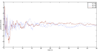
Figure 2: The evolution of tracking errors

5 Conclusions

In this paper we have studied the leader following problem of a multi-agent system with measurement noises and directed interconnection topology. The neighbor-based distributed control scheme with distributed estimators has been developed. Algebraic graph theory and stochastic analysis have been employed to analyze the mean square convergence of the tracking errors. One possible future research topic is to study the leader-following problem in a noisy environment when the dynamics of each agent is described by a more general linear system.

References

- Wang P. K. C., (1991) Wang P. K. C. (1991). Navigation strategies for multiple autonomous mobile robots moving in formation, J. Robot. Syst., vol. 8, no. 2, 177-195.
- Das,FierroKumar, (2002) Das A. K., Fierro R., Kumar V., et al. (2002). A vision-based formation control framework, IEEE trans. Robot. Autom., vol. 18, no. 5, 813-825.
- Vanek,Peni,et al., (2005) Vanek B., Peni T., Bokor J., Balas G. (2005). Practical approach to real-time trajectory tracking of UAV formations, in Proc. of American Control Conference, Oregon, 122-127.
- Anderson,Fidan,et al., (2008) Anderson B. D. O., Fidan B., Yu C., Walle D. (2008). UAV formation control: theory and application, Lecture Notes in Control and Information Sciences, Springer: Berlin, 371, 15-33.
- Gupta,CaoHaering, (2008) Gupta H., Cao X., Haering N. (2008). Map-based active leader-follower surveillance system, in Proc. of ECCV workshop on Multi-Camera and Multi-modal Sensor Fusion Algorithms and Applications, Marseille, France.
- HuHu, (2008) Hu J., Hu X. (2008). Optimal target trajectory estimation and filtering using networked sensors. Jr. Systems Science Complexity, vol. 21, 325-336.
- Jadbabaie,LinMorse, (2003) Jadbabaie A., Lin J., Morse A. S. (2003). Coordination of groups of mobile autonomous agents using nearest neighbor rules, IEEE Trans. on Automatic Control, vol. 48, no. 6, 988-1001.
- RenBeard, (2005) Ren W. Beard R. W. (2005). Consensus seeking in multiagent systems under dynamically changing interaction topologies, IEEE Trans. on Automatic Control, vol. 50, no. 5, 655-661.
- Lin,FrancisMaggiore, (2005) Lin Z., Francis B., Maggiore M. (2005). Necessary and sufficient graphical conditions for formation control of unicycles, IEEE Trans. on Automatic Control, vol. 50, no. 1, 121-127.
- ShiHong, (2009) Shi G., Hong Y. (2009). Global target aggregation and state agreement of nonlinear multi-agent systems with switching topologies, Automatica, vol. 45, no. 5, 1165-1175.
- HuHong, (2007) Hu J., Hong Y. (2007). Leader-following coordination of multi-agent systems with coupling time delays, Physica A, vol. 374, no. 2, 853-863.
- Lin,Jia, et al., (2008) Lin P., Jia Y., Du J., Yuan S. (2008). Distributed control of multi-agent systems with second-order agent dynamics and delay-dependent communications, Asian J. Control, vol. 10, no. 2, 254-259.
- FaxMurray, (2004) Fax A., Murray R. M., (2004). Information flow and cooperative control of vehicle formations. IEEE Trans. on Automatic Control, vol. 49, no. 9, 1465-1476.
- Hong,HuGao, (2006) Hong Y., Hu J.,, Gao L. (2006). Tracking control for multi-agent consensus with an active leader and variable topology, Automatica, vol. 42, no. 7, 1177-1182.
- LiZhang, (2009) Li T., Zhang J. F. (2009). Mean square average consensus under measurement noises and fxed topologies: necessary and sufficient conditions, Automatica, vol. 45, no. 8, 1929-1936.
- HuangManton, (2009) Huang M., Manton J. H. (2009), Coordination and consensus of networked agents with noisy measurement: stochastic algorithms and asymptotic behavior, SIAM Journal on Control and Optimization, vol. 48, no. 1, 134-161.
- GodsilRoyle, (2001) Godsil C., Royle G. (2001). Algebraic Graph Theory, New York: Springer-Verlag.
- NevelsonHasminskii, (1976) Nevelson M. B., Hasminskii R. Z. (1976). Stochastic Approximation and Recursive Estimation, Providence : American Mathematical Society.
- ChowTeicher, (1997) Chow Y. S., Teicher H. (1997). Probability theory: independence, interchangeability, martingales, New York: Springer.
- Friedman A., (1975) Friedman A. (1975). Stochastic differential equations and applications: Vol. 1, New York: Academic Press.
- MichelMiller, (1977) Michel A. N., Miller R. K. (1977) Qualitative analysis of large scale dynamical systems, New York: Academic Press.