All-order evaluation of weak measurements
— The cases of an operator ${\bf A}$ which satisfies the property ${\bf A}^{2}=1$ —

Abstract

Some exact formulae of the expectation values and probability densities in a weak measurement for an operator ${\bf A}$ which satisfies the property ${\bf A}^{2}=1$ are derived. These formulae include all-order effects of the unitary evolution due to the von-Neumann interaction. These are valid not only in the weak measurement regime but also in the strong measurement regime and tell us the connection between these two regime. Using these formulae, arguments of the optimization of the signal amplification and the signal to noise ratio are developed in two typical experimental setups.

I Introduction

Since the proposal of the weak measurement by Aharonov, Albert, and Vaidman (AAV) Y.Aharonov-D.Z.Albert-L.Vaidman-1988 in 1988, weak measurements have been investigated by many researchers. The idea of weak measurement has been used to resolve fundamental paradoxes in quantum mechanics such as Hardy’s paradox Y.Aharonov-A.Botero-S.Pospescu-B.Reznik-J.Tollaksen-2001 . In addition to many theoretical works on weak measurements, it is important to note that some experiments realized this weak measurement in different experimental setups N.W.M.Ritchie-J.G.Story-R.G.Hulet-1991 ; G.J.Pryde-J.L.O'Brien-A.G.White-T.C.Ralph-H.M.Wiseman-2005 ; O.Hosten-P.Kwiat-2008 ; P.B.Dixon-D.J.Starling-A.N.Jordan-J.C.Howell-2009 ; M.Iinuma-Y.Suzuki-G.Taguchi-Y.Kadoya-H.F.Hofmann-2011 . These experiments show that the weak measurement is also very useful for high-precision measurements. For example, Hosten and Kwiat O.Hosten-P.Kwiat-2008 used the weak measurement to observe a tiny spin Hall effect in light; Dixon et al. P.B.Dixon-D.J.Starling-A.N.Jordan-J.C.Howell-2009 ; D.J.Starling-P.B.Dixon-A.N.Jordan-J.C.Howell-2009 (DSJH) used the weak measurement to detect very small transverse beam deflections. The original AAV work Y.Aharonov-D.Z.Albert-L.Vaidman-1988 also includes the proposal of the application to the sequence of the Stern-Gerlach experiments for spin-1/2 particles. They claim that we can observe the spin of particles as a larger value than the range of its eigenvalues. This is called “weak-value amplification”. The above high-precision measurements using the weak measurement are due to the effect of this weak-value amplification.

Weak measurements are based on von-Neumann’s measurement theory J.von-Neumann-1932 in which the total system consists of the system to be measured and a detector to measure the system. Further, we specify the initial state (pre-selection) and the final state (post-selection) of the system. AAV also proposed the situation of the measurement, in which the initial variance in the momentum conjugate to the pointer variable of the detector is so small that the interaction between the system and the detector is very weak Aharonov-Vaidman-2007-update-review . Because of this weakness, the measurement proposed by AAV is called “weak measurement”. In the linear-order of the interaction between the system and detector, the outcome of the weak measurements is so-called “weak value”. The weak-value amplification is essentially due to the fact that the weak value of an quantum observable may become larger than eigenvalues of this observable when the pre- and the post-selection is nearly orthogonal. Due to the weakness of the interaction between the system and the detector, the measurement by a single ensemble is imprecise. However, as noted by Aharonov and Vaidman Aharonov-Vaidman-2007-update-review , the measurement become precise by a factor $\sqrt{N}$ through performing large $N$ ensemble experiments.

Measurements of arbitrary strength beyond the linear-order interaction has been first discussed by Aharonov and Botero Y.Aharonov-A.Botero-2005 in the context of the framework called “Quantum average of weak value.” In this framework, the strong measurement of a pointer variable can be regarded as quantum superpositions of weak measurements. They applied their framework to a specific case of a spin measurement. Furthermore, all-order effects of the unitary evolution due to the von-Neumann interaction between the system and the detector are also investigated by investigated by Di Lorenzo and Euges A.D.Lorenzo-J.C.Egues-2008 in AAV setup to clarify the detector dynamics in weak masurements.

More recently, Wu and Li S.Wu-Y.Li-2010 proposed the general formulation of the weak measurement which includes all-order effects of the unitary evolution due to the von-Neumann interaction between the system and the detector. Through this formulation, they took some higher-order effects into account when they computed the shift of pointer variables and pointed out that there is a overlap of the pre- and the post-selection at which the outcome of the weak measurement have the maximal amplification. However, since they did not take all higher-order effects into account, their claim on the maximal amplification is weak.

In this paper, we carry out the all-order evaluation of some expectation values of pointer variables after the post-selection based on the formulation proposed by Wu and Li S.Wu-Y.Li-2010 . Although the all-order evaluations of the expectation values in general weak measurement are difficult, these evaluations are possible if we concentrate only on the weak measurements for an operator ${\bf A}$ of the system which satisfies the property ${\bf A}^{2}=1$. Choosing the initial state of the detector as a zero mean-value Gaussian state, we derive some formulae of the expectation values and probability densities for the detector after the post-selection without any approximation. Through these formulae, we discuss the maximal amplification which suggested by Wu and Li.

Although our consideration is restricted only to the case of the weak measurement for an operator ${\bf A}$ which satisfies the property ${\bf A}^{2}=1$, this case includes many experimental setups. For example, the weak measurement of the spins of spin-1/2 particles, which was originally proposed by AAV Y.Aharonov-D.Z.Albert-L.Vaidman-1988 , is included since the Pauli spin matrices satisfy the property ${\bf A}^{2}=1$. The experiment by Hosten-Kwiat O.Hosten-P.Kwiat-2008 and the experimental setup by DSJH P.B.Dixon-D.J.Starling-A.N.Jordan-J.C.Howell-2009 are also included in our case, though there are some additional modification in their actual experimental setups. Thus, our consideration will be applicable to many experimental setups. Therefore, it is worthwhile to research the weak measurements for an operator ${\bf A}$ which satisfies the property ${\bf A}^{2}=1$.

Furthermore, we note that some experiments of weak measurement for an operator ${\bf A}$ which satisfies the property ${\bf A}^{2}=1$ are classified into two types: one is the weak measurements with a real weak value; and the other is those with a weak value of pure imaginary. A typical example of the weak measurement with a real weak value is the experimental setup of a spin-1/2 particle proposed by AAV Y.Aharonov-D.Z.Albert-L.Vaidman-1988 . On the other hand, a typical example of the weak measurement with a weak value of pure imaginary is the DSJH experiment P.B.Dixon-D.J.Starling-A.N.Jordan-J.C.Howell-2009 . We apply our results of all-order evaluations to these two specific experimental setups. Then, we discuss the optimizations of the expectation value of the pointer variable of the detector (i.e., the signal optimization) and the optimization of the signal to noise ratio (SNR). Through these applications, we concretely discuss the maximum amplification in the weak measurements.

Organization of this paper is as follows: In Sec. II, we briefly review the general formulation proposed by Wu and Li. In Sec. III, we summarize the formulae for some expectation values and probability densities which are derived from all-order evaluations through Wu-Li formulation. In Sec. IV, the application of our formulae to AAV setup is discussed. In Sec. V, we discuss the application of our formulae to DSJH setup, though the experimental setup in this paper is a simpler version of the original DSJH setup. Final section (Sec. VI) is devoted to the summary.

Throughout this paper, we use the natural unit $\hbar=1$.

II Wu-Li Formalism

Here, we review the description of weak measurements proposed by Wu and Li S.Wu-Y.Li-2010 . In Sec. II.1, we first review the general framework of the weak measurement following Ref. S.Wu-Y.Li-2010 . To carry out the analyses, we must treat two cases separately for a technical reason. One is the case where the initial and the final states of the system is not orthogonal, which is described in Sec. II.2. The other is the case where the initial and the final states of the system is orthogonal, which is described in Sec.II.3.

II.1 General framework

The total system we consider here is described by the density matrix $\rho=\rho_{s}\otimes\rho_{d}$. $\rho_{s}$ is the density matrix of the “system” which is a quantum system and we measure an observable ${\bf A}$ associated with this system. $\rho_{d}$ is the density matrix of the “detector” which interacts with the system through the von-Neumann interaction

$${\cal H}=g\delta(t-t_{0}){\bf A}\otimes p.$$ (1)

Here, $p$ is the conjugate momentum to the pointer variable $q$ of the detector, i.e., $[q,p]=i$. In the usual von-Neumann interaction (strong interaction), the eigenvalues of ${\bf A}$ appear in the pointer variable $q$ J.von-Neumann-1932 . Using these three elements, the weak measurement is carried out through the sequence of four measurements Y.Aharonov-D.Z.Albert-L.Vaidman-1988 . First three processes of these four measurements are called “pre-selection”, “weak interaction”, “post-selection”. The final one is the measurement of the detector pointer variable through any type of the measurement in quantum mechanics.

First, we prepare the initial state $\rho_{s}$ of the system through the projection measurement at $t<t_{0}$, which is called “pre-selection”. We also prepare the initial state of the detector $\rho_{d}$. After this pre-selection, the system and the detector interact with each other through the interaction Hamiltonian (1). The time evolution through this interaction is described by the evolution operator ${\cal U}=e^{-ig{\bf A}p}$ and the total density matrix $\rho$ evolves as

$$\rho^{\prime}={\cal U}\rho{\cal U}^{\dagger}=\rho+\sum_{n=1}^{+\infty}\frac{(-ig)^{n}}{n!}{\bf ad}^{n}p{\bf A}\circ\rho,$$ (2)

where ${\bf ad}^{n}$ for arbitrary operators $\Omega$ and $\Theta$ is recursively defined as

$${\bf ad}^{1}\Omega\circ\Theta := {\bf ad}\Omega\circ\Theta=\left[\Omega,\Theta\right],$$ (3)

$${\bf ad}^{n}\Omega\circ\Theta := {\bf ad}\Omega\circ({\bf ad}^{n-1}\Omega\circ\Theta)$$ (4)

$$= \left[\Omega,{\bf ad}^{n-1}\Omega\circ\Theta\right].$$

The prime in Eq. (2) denotes the operator after the interaction (1). The density matrix of the system after this interaction is given by

$$\rho^{\prime}_{s}={{\mbox{Tr}}}_{d}\rho^{\prime}=\rho_{s}+\sum_{n=1}^{+\infty}\frac{(-ig)^{n}}{n!}\langle p^{n}\rangle{\bf ad}^{n}{\bf A}\circ\rho_{s},$$ (5)

where ${{\mbox{Tr}}}_{d}$ means taking the trace of the detector density matrix and $\langle p^{n}\rangle:={{\mbox{Tr}}}_{d}(p^{n}\rho_{d})$. Equation (5) implies that the density matrix of the system hardly changes through the interaction with the detector if $g\sup\{\langle p^{n}\rangle^{1/n},n\in{{\mathbb{N}}}\}\ll 1$. Roughly speaking, this condition is regarded as $g\Delta p\ll 1$, where $(\Delta p)^{2}$ is the variance in $p$, and is interpreted that the interaction between the system and the detector in the measurement is “weak interaction”. After this interaction, we restrict the final state of the system by the projection operator $\Pi_{f}$: $\rho^{\prime}\rightarrow\rho^{\prime}\Pi_{f}$. This restriction is called “post-selection”. The density matrix of the detector after the post-selection is given by

$$\rho_{d}^{\prime}=\frac{{{\mbox{Tr}}}_{s}\rho^{\prime}\Pi_{f}}{{{\mbox{Tr}}}\rho^{\prime}\Pi_{f}},$$ (6)

where ${{\mbox{Tr}}}_{s}$ (Tr) means taking the trace of the system density matrix (the total density matrix).

Although $\rho_{s}$ and $\rho_{d}$ may describe mixed states of the system and the detector, we restrict our attention to pure states as the initial density matrices $\rho_{s}$ and $\rho_{d}$. We denote these initial density matrices as $\rho_{s}=|\psi_{i}\rangle\langle\psi_{i}|$ and $\rho_{d}=|\phi\rangle\langle\phi|$. Further, we also denote the projection operator for the post-selection by $\Pi_{f}:=|\psi_{f}\rangle\langle\psi_{f}|$. In this case, the normalization factor (${{\mbox{Tr}}}\rho^{\prime}\Pi_{f}$) of the density matrix of the detector after the post-selection is given by

$${{\mbox{Tr}}}\rho^{\prime}\Pi_{f} = \left|\langle\psi_{f}|\psi_{i}\rangle\right|^{2}+\sum_{n=1}^{+\infty}\frac{(-ig)^{n}\langle p^{n}\rangle}{n!}\sum_{k=0}^{n}(-1)^{k}{}_{n}C_{k}$$ (7)

$$\quad\quad\quad\quad\quad\times\langle\psi_{f}|{\bf A}^{n-k}|\psi_{i}\rangle\langle\psi_{i}|{\bf A}^{k}|\psi_{f}\rangle,$$

where $\langle p^{n}\rangle=\langle\phi|p^{n}|\phi\rangle$ and ${}_{n}C_{k}$ is the binomial coefficient.

To carry out the further analyses, the factor $\left|\langle\psi_{f}|\psi_{i}\rangle\right|$ plays an important role and separate treatments are required according to the fact whether $\left|\langle\psi_{f}|\psi_{i}\rangle\right|=0$ or not.

II.2 Non-orthogonal weak measurement $\left|\langle\psi_{f}|\psi_{i}\rangle\right|\neq 0$

Here, we consider the case where the pre- and post-selection are not orthogonal, i.e., $\left|\langle\psi_{f}|\psi_{i}\rangle\right|\neq 0$. In this case, the trace of the post-selected density matrix and the density matrix $\rho_{d}^{\prime}$ after the post-selection are given by

$${{\mbox{Tr}}}\rho^{\prime}\Pi_{f} =: \left|\langle\psi_{f}|\psi_{i}\rangle\right|^{2}{\cal Z},$$ (8)

$${\cal Z} = 1+\sum_{n=1}^{+\infty}\frac{(-ig)^{n}\langle p^{n}\rangle}{n!}$$

$$\quad\quad\times\sum_{k=0}^{n}(-1)^{k}{}_{n}C_{k}\langle{\bf A}^{n-k}\rangle_{w}\langle{\bf A}^{k}\rangle_{w}^{*},$$

(9)

$${\cal Z}\rho_{d}^{\prime} = \rho_{d}+\sum_{n=1}^{+\infty}\frac{(-ig)^{n}}{n!}\sum_{k=0}^{n}(-1)^{k}{}_{n}C_{k}$$

$$\quad\quad\quad\times\langle{\bf A}^{n-k}\rangle_{w}\langle{\bf A}^{k}\rangle_{w}^{*}p^{n-k}\rho_{d}p^{k},$$

where $\langle\cdot\rangle_{w}:=\langle\psi_{f}|\cdot|\psi_{i}\rangle/\langle\psi_{f}|\psi_{i}\rangle$.

When the wave function $\langle p|\phi\rangle$ is even in $p$, i.e., $\langle p^{n}\rangle=0$ for odd $n$, Wu and Li derived the formulae of the shifts in $q$ and $p$ as

$$\delta q = \frac{g\Re{\bf A}_{w}+g\Im{\bf A}_{w}\langle\left\{q,p\right\}\rangle}{1+g^{2}\langle p^{2}\rangle\left(\left|{\bf A}_{w}\right|^{2}-\Re\langle{\bf A}^{2}\rangle_{w}\right)},$$ (11)

$$\delta p = \frac{2g\Im{\bf A}_{w}\langle p^{2}\rangle}{1+g^{2}\langle p^{2}\rangle\left(\left|{\bf A}_{w}\right|^{2}-\Re\langle{\bf A}^{2}\rangle_{w}\right)},$$ (12)

where $\delta q:={{\mbox{Tr}}}(q\rho_{d}^{\prime})-{{\mbox{Tr}}}(q\rho_{d})$ and $\delta p:={{\mbox{Tr}}}(p\rho_{d}^{\prime})-{{\mbox{Tr}}}(p\rho_{d})$. In their derivation, they neglect terms of $O(g^{3})$ in the numerators and the denominators, but they do not expand the total expressions (11) and (12) in form of the power series of $g$. Although these treatments of $\delta q$ and $\delta p$ might be regarded as some renormalization technique, it is also true that the expressions (11) and (12) include only partial effects of higher order of $g$.

As pointed out by AAV Y.Aharonov-D.Z.Albert-L.Vaidman-1988 , weak values may become very large in the limit $\left|\langle\psi_{f}|\psi_{i}\rangle\right|\rightarrow 0$ ($\neq 0$). At the order of $O(g)$, the shifts (11) and (12) are proportional to the weak value $\langle{\bf A}\rangle_{w}$ R.Jozsa-2007 . This implies that the shifts (11) and (12) of order $O(g)$ may diverge in the limit $\left|\langle\psi_{f}|\psi_{i}\rangle\right|\rightarrow 0$. This is the essence of the weak value amplification. However, from the total expressions of Eqs. (11) and (12), Wu and Li suggested that, in the limit $\left|\langle\psi_{f}|\psi_{i}\rangle\right|\rightarrow 0$, these shifts decrease rapidly when $\left|{\bf A}_{w}\right|^{2}$ become comparable with $(g^{2}\langle p^{2}\rangle)^{-1}$. This arguments implies that, for a fixed $g^{2}\langle p^{2}\rangle$, there may exist a maximum shift of a pointer quantity, and an optimal overlap $\left|\langle\psi_{f}|\psi_{i}\rangle\right|$ to achieve the maximum shift. We call this overlap as the optimal pre-selection (or optimal post-selection).

Although Wu and Li claim is weak in the sense that they did not take all higher-order effects into account, in this paper, we show that their claim on the optimal pre-selection is essentially correct through the all-order evaluation of weak measurements for an operator ${\bf A}$ which satisfies the property ${\bf A}^{2}=1$.

II.3 Orthogonal weak measurement $\left|\langle\psi_{f}|\psi_{i}\rangle\right|=0$

Next, we consider the orthogonal case where $\left|\langle\psi_{f}|\psi_{i}\rangle\right|=0$. In this case, the original formalism of the weak measurement fails and the weak values are not defined. This is easily seen from the fact that the normalization factor ${\cal Z}$ defined by Eq. (8) is ill-defined. However, instead of ${\cal Z}$, Wu and Li defined ${\cal Z}_{o}$ by

$${{\mbox{Tr}}}\rho^{\prime}\Pi_{f}=:g^{2}\langle p^{2}\rangle\left|\langle\psi_{f}|{\bf A}|\psi_{i}\rangle\right|^{2}{\cal Z}_{o},$$ (13)

$${\cal Z}_{o} = 1+\sum_{n=1}^{+\infty}\frac{(-ig)^{n}}{n!}\frac{\langle p^{n+2}\rangle}{\langle p^{2}\rangle}$$

$$\quad\quad\times\sum_{k=0}^{n}(-1)^{k}{}_{n}\!C_{k}\langle{\bf A}^{n-k}\rangle_{ow}\langle{\bf A}^{k}\rangle_{ow}^{*},$$

where

$$\langle{\bf A}^{n}\rangle_{ow}:=\frac{\langle\psi_{f}|{\bf A}^{n+1}|\psi_{i}\rangle}{\langle\psi_{f}|{\bf A}(n+1)|\psi_{i}\rangle}.$$ (15)

Wu and Li called $\langle{\bf A}^{n}\rangle_{ow}$ defined by Eq. (15) as orthogonal weak values. The density matrix of the detector after the post-selection is given by

$${\cal Z}_{o}\langle p^{2}\rangle\rho_{d}^{\prime} = p\rho_{d}p$$ (16)

$$+\sum_{n=1}^{+\infty}\frac{(-ig)^{n}}{n!}\sum_{k=0}^{n}(-1)^{k}{}_{n}\!C_{k}\langle{\bf A}^{n-k}\rangle_{ow}\langle{\bf A}^{k}\rangle_{ow}^{*}$$

$$\quad\quad\quad\times p^{n-k+1}\rho_{d}p^{k+1}.$$

From this expression (16), Wu and Li claim that the orthogonal weak values (15) play the similar role to the original weak values in non-orthogonal case.

III All-order evaluation of weak measurements for an operator ${\bf A}$ which satisfies ${\bf A}^{2}=1$

Here, we evaluate the density matrix of the detector after the post-selection and some expectation values in the case for an operator ${\bf A}$ which satisfies the property ${\bf A}^{2}=1$ based on the Wu-Li formalism. In addition to the restriction of our consideration to the simple operator case, in this section, we assume that the initial state $\rho_{d}=|\phi\rangle\langle\phi|$ of the detector is zero mean-value Gaussian, i.e.,

$$\langle p|\phi\rangle=\left(\frac{1}{2\pi\langle p^{2}\rangle}\right)^{1/4}\exp\left[-\frac{p^{2}}{4\langle p^{2}\rangle}\right].$$ (17)

From this initial state of the detector, we can easily derive the properties of the initial state:

$$\langle p^{2n+1}\rangle=0,\quad\langle p^{2n}\rangle=(2n-1)!!\langle p^{2}\rangle^{n}.$$ (18)

As reviewed in the last section II, according to the norm $\left|\langle\psi_{f}|\psi_{i}\rangle\right|^{2}$, we have to treat the density matrix in different way. Therefore, we treat a non-orthogonal weak measurement and an orthogonal one, separately.

III.1 Non-orthogonal weak measurement $\left|\langle\psi_{f}|\psi_{i}\rangle\right|\neq 0$

When the initial state of the detector is zero mean-value Gaussian (17), the moments of $p$ are given by Eqs. (18). In this case, the normalization ${\cal Z}$ [Eq. (85)] is given by

$${\cal Z}=1+\frac{1}{2}\left(1-\left|\langle{\bf A}\rangle_{w}\right|^{2}\right)\left(e^{-s}-1\right),$$ (19)

where $s$ is a parameter defined by

$$s:=2g^{2}\langle p^{2}\rangle.$$ (20)

Similar calculations lead the expectation values of $p$ and $q$ after the post-selection

$$\frac{\langle q\rangle^{\prime}}{g} = \frac{\Re\langle{\bf A}\rangle_{w}}{{\cal Z}},$$ (21)

$$g\langle p\rangle^{\prime} = \frac{se^{-s}\Im\langle{\bf A}\rangle_{w}}{{\cal Z}}.$$ (22)

[Here, we denotes the expectation value of $*$ for the detector after the post-selection by $\langle*\rangle^{\prime}$. Fluctuations $\Delta q:=\sqrt{\langle(q-\langle q\rangle^{\prime})^{2}\rangle^{\prime}}$ and $\Delta p:=\sqrt{\langle(p-\langle p\rangle^{\prime})^{2}\rangle^{\prime}}$ in $p$ and $q$ after the post-selection are given by

$$\frac{(\Delta q)^{2}}{g^{2}} = \frac{1}{2s}+\frac{1}{2{\cal Z}}\left(1+\left|\langle{\bf A}\rangle_{w}\right|^{2}\right)$$ (23)

$$-\frac{\left(\Re\langle{\bf A}\rangle_{w}\right)^{2}}{{\cal Z}^{2}},$$

$$g^{2}(\Delta p)^{2} = \frac{s}{2}-\frac{s^{2}e^{-s}}{2{\cal Z}}\left(1-\left|\langle{\bf A}\rangle_{w}\right|^{2}\right)$$ (24)

$$-\frac{s^{2}e^{-2s}(\Im\langle{\bf A}\rangle_{w})^{2}}{{\cal Z}^{2}}.$$

Further, the probability densities in $p$-space and $q$-space are given by

$$\langle p|\rho_{d}^{\prime}|p\rangle = \left[2+\left(1-\left|\langle{\bf A}\rangle_{w}\right|^{2}\right)\left(\cos(2gp)-1\right)\right.$$ (25)

$$\;\;\left.+2\Im\langle{\bf A}\rangle_{w}\sin(2gp)\frac{}{}\right]\frac{\langle p|\rho_{d}|p\rangle}{2{\cal Z}},$$

$$\langle q|\rho_{d}^{\prime}|q\rangle = \left[\frac{}{}1-\left|\langle{\bf A}\rangle_{w}\right|^{2}\right.$$ (26)

$$\;\;\left.+\left(1+\left|\langle{\bf A}\rangle_{w}\right|^{2}\right)\cosh\left(\frac{2sq}{g}\right)\right.$$

$$\;\;\left.+2\Re\langle{\bf A}\rangle_{w}\sinh\left(\frac{2sq}{g}\right)\right]$$

$$\quad\quad\quad\quad\times\frac{e^{-s}\langle q|\rho_{d}|q\rangle}{2{\cal Z}}.$$

where $\langle p|\rho_{d}|p\rangle$ and $\langle q|\rho_{d}|q\rangle$ are Gaussian initial probability densities

$$\langle p|\rho_{d}|p\rangle = \sqrt{\frac{g^{2}}{\pi s}}\exp\left[-\frac{(gp)^{2}}{s}\right],$$ (27)

$$\langle q|\rho_{d}|q\rangle = \sqrt{\frac{s}{\pi g^{2}}}\exp\left[-s\left(\frac{q}{g}\right)^{2}\right].$$ (28)

The derivation of Eq. (26) is explained in Appendix A.1.

Here, we note that the parameter $s$ defined in Eq. (20) is a measure of the strength of the interaction. Usually, it is said that the interaction between the system and the detector is weak if the coupling constant $g$ is very small. On the other hand, in the weak measurement Aharonov-Vaidman-2007-update-review , it is said that the interaction between the system and the detector is weak if the initial variance of the pointer variable $q$ is very large, i.e., the variance in the conjugate momentum $p$ is very small. These two concepts of the “weakness” of the measurement are automatically represented by the single non-dimensional parameter $s$. We call $s$ as the coupling parameter, and say that the interaction between the system and the detector is weak if $s\ll 1$ and strong if $s\gg 1$.

We have to emphasize that our formulae shown here are the results from the all-order evaluation of $s$ and valid not only in the weak measurement regime $s\ll 1$ but also in the strong measurement regime $s\gg 1$. The results coincide with those of the measurement in the strong regime. This situation can be observed through the specific experimental setups discussed in Sec. IV.

Finally, we note that probability distributions for weak measurements (both in the strong and weak regime) are first discussed by Aharonov and Botero Y.Aharonov-A.Botero-2005 in the context of the framework called “Quantum averages of weak value” as mentioned in Sec. I. Of course, our formulae of the probability distribution shown in this paper are not general because we concentrate only on the case of an operator ${\bf A}$ which satisfies the property ${\bf A}^{2}=1$. However, as emphasize in Sec. I, many experimental setups are included in this special case and we have derived explicit simple analytic formulae for this special case. This is one of main points of this paper.

III.2 Orthogonal weak measurement $\left|\langle\psi_{f}|\psi_{i}\rangle\right|=0$

Now, we consider the orthogonal case where the pre-selected state and the post-selected state are orthogonal to each other, i.e., $\langle\psi_{f}|\psi_{i}\rangle=0$. As reviewed in Sec. II.3, the density matrix of the detector after the post-selection is given by Eq. (16). In the case of the weak measurements for the operator ${\bf A}$ with the property ${\bf A}^{2}=1$, the orthogonal weak values (15) are given by

$$\langle{\bf A}^{n}\rangle_{ow}=\left\{\begin{array}[]{ccc}\displaystyle\frac{1}{n+1}&\mbox{for}&n\;\;\mbox{is even},\\ 0&\mbox{for}&n\;\;\mbox{is odd}.\end{array}\right.$$ (31)

This expression implies that no information of ${\bf A}$ appears in the orthogonal weak measurement for an operator ${\bf A}$ with the property ${\bf A}^{2}=1$.

Through the Gaussian initial state (17) of the detector with the properties (18), the normalization constant ${\cal Z}_{o}$ defined by Eq. (LABEL:eq:S.Wu-Y.Li-2010-22) is given by

$${\cal Z}_{o} = \frac{4}{s}\left(1-e^{-s}-\frac{3}{4}s\right),$$ (32)

where the coupling parameter $s$ is defined in Eq. (20). The density matrix (16) of the detector after the post-selection is given by

$${\cal Z}_{o}\langle p^{2}\rangle\rho_{d}^{\prime} = p\rho_{d}p+\sum_{n=1}^{+\infty}\frac{(-ig)^{2n}}{(2n+2)!}\sum_{k=0}^{n}{}_{2n+2}C_{2k+1}$$ (33)

$$\quad\quad\quad\quad\quad\times p^{2n-2k+1}\rho_{d}p^{2k+1}.$$

In the case where the initial state of the detector is zero mean-value Gaussian (17), the expectation value of $p$ after the post-selection, which is evaluated in Appendix A.2, is trivial,

$$\langle p\rangle^{\prime}=0,$$ (34)

due to the properties (18). Further, in Appendix A.2, we also show that the expectation value of $q$ [Eq. (117)] after the post-selection also yields a trivial result

$$\langle q\rangle^{\prime}=0.$$ (35)

As shown in Appendix A.2, the fluctuations $\Delta p$ and $\Delta q$ in $p$ and $q$ of the detector after the post-selection are given by

$$g^{2}(\Delta p)^{2} = \frac{s}{2}\frac{1+(2s-1)e^{-s}}{4-3s-4e^{-s}}.$$ (36)

$$\frac{(\Delta q)^{2}}{g^{2}} = \frac{1}{2s}\frac{1-e^{-s}+4s}{4-4e^{-s}-3s}.$$ (37)

The probability densities in $p$-space and in $q$-space are given by

$$\langle p|\rho_{d}^{\prime}|p\rangle = \frac{1-\cos(2gp)}{2\left(4-4e^{-s}-3s\right)}\langle p|\rho_{d}|p\rangle,$$ (38)

$$\langle q|\rho_{d}^{\prime}|q\rangle = \frac{2e^{-s}\sinh^{2}\left(sq/g\right)}{4-4e^{-s}-3s}\langle q|\rho_{d}|q\rangle,$$ (39)

respectively. Here, $\langle p|\rho_{d}|p\rangle$ and $\langle q|\rho_{d}|q\rangle$ are the Gaussian initial probability densities (27) and (28), respectively. The derivations of these formulae are given in Appendix A.2.

Thus, both in the non-orthogonal weak measurements (Sec. III.1) and the orthogonal one (Sec. III.2), we explicitly derived the analytical expressions of the expectation values of $p$ and $q$, fluctuations in $p$ and $q$, and the probability distributions in $p$-space and in $q$-space for the detector only under two assumptions, i.e., the operator ${\bf A}$ for the system satisfies the property ${\bf A}^{2}=1$ and the initial state of the detector is zero mean-value Gaussian (17).

We note that the formulae (21) and (22) for the expectation values for $p$ and $q$ coincide with Eqs. (11) and (12), respectively, if we ignore the higher-order terms of than $O(g^{2})$. In this sense, equations (21) and (22) are all-order extension of Eqs. (11) and (12) derived by Wu and Li S.Wu-Y.Li-2010 . We also note that the expressions of Eqs. (21) and (22) are valid for arbitrary value of the coupling parameter $s$. Furthermore, the behaviors of Eqs. (21) and (22) are qualitatively same as those of Eqs. (11) and (12). Therefore, we may say that the claim on the optimal post-selection proposed by Wu and Li is essentially correct and mathematically justified by Eqs. (21) and (22).

In the following two sections, we apply the formulae summarized in this section to two specific experimental setups and examine the weak measurement of these two setups in detail. Since we already showed that the orthogonal weak measurement yields trivial results in the expectation value of $p$ and $q$, we concentrate only on the non-orthogonal weak measurement.

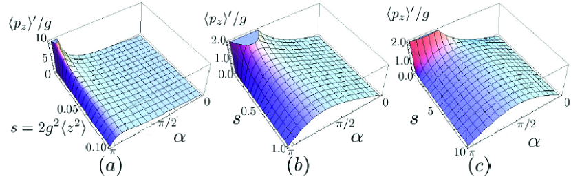
Figure 1: $\langle p_{z}\rangle^{\prime}/g$ is shown as a function of the coupling $s=2g^{2}\langle z^{2}\rangle$ and the pre-selection angle $\alpha$ in various range of $s$. (a) $s\in(0,0.1)$, (b) $s\in(0,1)$, (c) $s\in(0,10)$. From these figures, we can see that, for given coupling parameter $s$, there is a optimal pre-selection angle $\alpha$ such that the expectation value of $p_{z}$ is maximized.

IV Application to AAV setup

In this section, we apply our formulae derived in Sec. III to the AAV Y.Aharonov-D.Z.Albert-L.Vaidman-1988 setup. Through this application, we discuss the optimization of the expectation value of the signal and SNR.

IV.1 Setup of experiment

The experimental setup proposed by AAV Y.Aharonov-D.Z.Albert-L.Vaidman-1988 is the sequence of three Stern-Gerlach experiments for spin-1/2 particles.

The pre-selected state of the spin-1/2 particle is

$$|\uparrow_{\xi}\rangle=\frac{1}{\sqrt{2}}\left(\sqrt{1+\sin\alpha}|\uparrow_{z}\rangle+\sqrt{1-\sin\alpha}|\downarrow_{z}\rangle\right),$$ (40)

which is an eigenstate $\sigma_{\xi}|\uparrow_{\xi}\rangle=+|\uparrow_{\xi}\rangle$ of the operator $\sigma_{\xi}=\cos\alpha\sigma_{x}+\sin\alpha\sigma_{z}$.

The weak interaction in the weak measurement is described by the interaction Hamiltonian

$${\cal H}=-gz\otimes\sigma_{z}\delta(t-t_{0}),\quad g=\mu\left(\frac{\partial B_{z}}{\partial z}\right),$$ (41)

where $\mu$ is the magnetic moment of the spin-1/2 particle and $B_{z}$ is the $z$-component of the magnetic field. The pointer variable in this setup is $p_{z}$ which conjugate to $z$. We note that the operator ${\bf A}$ to be observed is the spin $z$-component of a spin-1/2 particle through the von-Neumann interaction (1), i.e.,

$${\bf A}=\sigma_{z}=|\uparrow_{z}\rangle\langle\uparrow_{z}|-|\downarrow_{z}\rangle\langle\downarrow_{z}|,$$ (42)

which satisfies the property ${\bf A}^{2}=1$. Then, we may apply our formulae provided in Sec. III.1. Comparing Eq. (41) with the interaction Hamiltonian (1), we find the correspondence of variables as

$$p\rightarrow-z,\quad q\rightarrow p_{z}.$$ (43)

The post-selection in this setup is

$$|\uparrow_{x}\rangle=\frac{1}{\sqrt{2}}\left(|\uparrow_{z}\rangle+|\downarrow_{z}\rangle\right)$$ (44)

which is an eigenstate $\sigma_{x}|\uparrow_{x}\rangle=+|\uparrow_{x}\rangle$ of the $x$-component $\sigma_{x}$ of the spin.

The weak value in this setup is given by

$$\langle{\bf A}\rangle_{w}=\frac{\langle\uparrow_{x}|\sigma_{z}|\uparrow_{\xi}\rangle}{\langle\uparrow_{x}|\uparrow_{\xi}\rangle}=\tan\frac{\alpha}{2},$$ (45)

where $\alpha$ is the pre-selection angle. We note that this weak value (45) is real.

IV.2 All-order expectation values and probability distribution

Here, we apply the formulae summarized in Sec. III.1 to the AAV setup. The normalization factor ${\cal Z}$ [Eq. (19)], is given by

$${\cal Z}=\frac{1+e^{-s}\cos\alpha}{1+\cos\alpha},$$ (46)

where $s$ is the coupling parameter [see Eq. (20)] defined by

$$s:=2g^{2}\langle z^{2}\rangle.$$ (47)

Expectation value of $p_{z}$ and $z$ are given by

$$\frac{\langle p_{z}\rangle^{\prime}}{g}=\frac{\sin\alpha}{1+e^{-s}\cos\alpha},\quad\langle z\rangle^{\prime}=0.$$ (48)

The expectation value of $\langle p_{z}\rangle^{\prime}/g$ is shown as a function of the coupling parameter $s$ and the pre-selection angle $\alpha$ in Fig. 1. In Fig. 1(a), we can see a pole at $(s,\alpha)=(0,\pi)$. Due to this pole, the weak value is amplified as pointed out by AAV. In the region $s\gg 1$, the expectation value (48) of $\langle p_{z}\rangle^{\prime}/g$ behaves $\langle p_{z}\rangle^{\prime}/g\sim\sin\alpha$. This behavior can be seen in Fig. 1(c). The qualitative difference between Eqs. (11)-(12) by Wu-Li and Eqs. (21)-(22) in this paper becomes large in the strong region $s\gg 1$.

Fluctuations $\Delta p_{z}$ and $\Delta z$ are given by

$$\frac{\left(\Delta p_{z}\right)^{2}}{g^{2}} = \frac{1}{2s}+\frac{\cos\alpha\left(\cos\alpha+e^{-s}\right)}{(1+e^{-s}\cos\alpha)^{2}},$$ (49)

$$g^{2}\left(\Delta z\right)^{2} = \frac{s}{2}-\frac{s^{2}e^{-s}\cos\alpha}{1+e^{-s}\cos\alpha}.$$ (50)

We also note that the first term in Eq. (49) [Eq. (50)] shows the initial variance in $p_{z}$ (in $z$). The remaining terms in Eqs. (49) and (50) are due to the pre-selection, weak interaction, and the post-selection.

The probability density of the detector after the post-selection in $p_{z}$-space is given by

$$\langle p_{z}|\rho_{d}^{\prime}|p_{z}\rangle = \frac{\cos\alpha+\cosh(2sp_{z}/g)+\sin\alpha\sinh(2sp_{z}/g)}{1+e^{-s}\cos\alpha}$$

$$\quad\times\exp[-s]\sqrt{\frac{s}{\pi g^{2}}}\exp\left[-s(p_{z}/g)^{2}\right].$$

Lorenzo and Egues A.D.Lorenzo-J.C.Egues-2008 also derived analytical formulae of the expectation of the pointer variable and the probability distribution in more complicated form. Their derivation is based on Born’s rule of the joint probability. Our results shown here are consistent with their results.

IV.3 Expectation value optimization

Figure 1 explicitly shows the existence of the ridge in the surface of the expectation value (48). This means that for a fixed coupling parameter $s$, there is the optimal pre-selection angle $\alpha$ at which the expectation value (48) is maximized. This was pointed out by Wu and Li S.Wu-Y.Li-2010 from the less accurate expression (11). On the other hand, we can accurately discuss this optimization of the expectation value from our exact expression (48). Here, we consider this optimization of the expectation value (48) in detail.

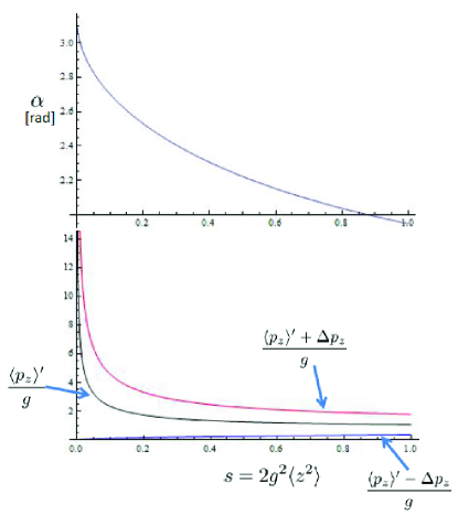
Figure 2: [Online Color] The optimal expectation-value line (52) [top panel], the expectation value $\langle p_{z}\rangle^{\prime}/g$ [Eq. (53)] and the fluctuation $\Delta p_{z}$ [Eq. (54)] in $p_{z}$ after the post-selection on the optimal line (52) [lower panel] are shown as functions of the coupling parameter $s$. We also show that $(\langle p_{z}\rangle^{\prime}\pm\Delta p_{z})/g$ in this lower panel. [The red line is $(\langle p_{z}\rangle^{\prime}+\Delta p_{z})/g$ and the blue line is $(\langle p_{z}\rangle^{\prime}-\Delta p_{z})/g$.] This figure shows that if we choose the small parameter of $s\ll 1$, we can accomplish the large expectation value of $\langle p_{z}\rangle^{\prime}/g\sim 1/\sqrt{2s}$, but the fluctuations in $p_{z}$ also amplified as $\Delta p_{z}/g\sim 1/\sqrt{2s}$.

To derive the points at which the expectation value is optimized, we consider the equation $\partial(\langle p_{z}\rangle^{\prime}/g)/\partial\alpha=0$. This equation yields

$$\cos\alpha=-e^{-s}.$$ (52)

We call the line which is expressed by Eq. (52) on the $(s,\alpha)$-plane as the optimal expectation-value line. On this optimal line, the expectation value of $p_{z}$ and the fluctuation $\Delta p_{z}$ in $p_{z}$ are given by

$$\frac{\langle p_{z}\rangle^{\prime}}{g} = \frac{1}{\sqrt{1-e^{-2s}}},$$ (53)

$$\frac{\Delta p_{z}}{g} = \frac{1}{\sqrt{2s}}.$$ (54)

Here, we note that the fluctuation $\Delta p_{z}$ (54) in $p_{z}$ coincides with that for the initial state of the detector. The optimal expectation-value line, the expectation value $\langle p_{z}\rangle^{\prime}$, and the fluctuation $\Delta p_{z}$ in $p_{z}$ on this optimal line are shown in Fig. 2.

The expectation value (53) of $p_{z}$ explicitly shows that we can accomplish the arbitrary large weak value amplification if we prepare the sufficiently small coupling parameter $s$. Actually, when $s\ll 1$, $\langle p_{z}\rangle^{\prime}\sim g/\sqrt{2s}=1/(2\sqrt{\langle z^{2}\rangle})$. Thus, the expectation value of $p_{z}$ can be very large if we choose the initial variance in $z$ is very small. This is just the weak value amplification proposed by AAV Y.Aharonov-D.Z.Albert-L.Vaidman-1988 .

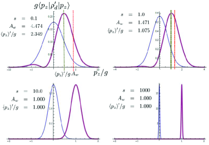
Figure 3: [Online Color] Probability distribution functions (55) in $p_{z}/g$-space on the optimal expectation-value line (52) with some coupling parameters $s$ are shown by the thick lines (red lines). We also plot the initial probability distribution $\sqrt{\frac{s}{\pi}}e^{-s(p_{z}/g)^{2}}$ with the same coupling parameter $s$ by the thin lines (blue lines). $s=0.1$ case corresponds to the weak measurement on the optimal expectation-value line (52). This shows that the peak of the probability distribution slightly deviates from the weak value $A_{w}$. $s=1.0$ case is still essentially same as $s=0.1$ case. $s=10$ and $s=1000$ cases correspond to the strong measurement case. These behaviors of the probability distribution (55) also well-describes the strong measurement regime $s\gg 1$.

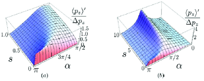
Figure 4: The signal to noise ratio (SNR) (56) is shown as a function of the coupling parameter $s$ and the pre-selection angle $\alpha$ : (a) $s\in(0,1)$ and $\alpha\in(\pi/2,\pi)$; (b) $s\in(0,10)$ and $\alpha\in(\pi,0)$. There is the ridge of the SNR from $(s,\alpha)=(0,\pi)$ to $(s,\alpha)=(+\infty,\pi/2)$. [We note that the direction of $s$-axes are opposite to those in Fig. 1.] The ridge around $\alpha=\pi/2$ is due to the strong measurement regime $s\gg 1$, which is due to the fact that $\alpha=\pi/2$ corresponds to the eigenstate $|\uparrow_{z}\rangle$ of the operator $\sigma_{z}$ with the eigenvalue $+1$. Together with Fig. (3), this shows the behavior of the SNR between the weak-measurement regime $s\ll 1$ and the strong-measurement regime $s\gg 1$.

On the optimal expectation-value line (52), the probability distribution (LABEL:eq:kouchan-A2is1-3.3.26-2) is given by

$$\langle p_{z}|\rho_{d}^{\prime}|p_{z}\rangle = \frac{\cosh(2sx)+\sqrt{1-e^{-2s}}\sinh(2sx)-e^{-s}}{1-e^{-2s}}$$ (55)

$$\quad\times\sqrt{\frac{s}{\pi g^{2}}}e^{-s(1+x^{2})},$$

where $x:=p_{z}/g$. This probability distribution on the optimal expectation-value line is shown in Fig. 3 with some coupling parameters $s$. In Fig. 3, $s=0.1$ case corresponds to the weak measurement on the optimal expectation-value line (52). This shows that the peak of the probability distribution slightly deviates from the weak value $A_{w}$ and the probability density after the post-selection is slightly different from the Gaussian profile I.M.Duck-P.M.Stevenson-E.C.G.Sudarshan-1989 . $s=1.0$ case is still essentially same as $s=0.1$ case. $s=10$ and $s=1000$ cases correspond to the strong measurement regime. On the optimal expectation-value line (52), $\alpha$ approaches to $\pi/2$ in the limit $s\rightarrow\infty$ and $\Delta p_{z}$ in Eq. (54) approaches to $0$. Here, we note that the pre-selected state with $\alpha=\pi/2$ corresponds to the eigenstate $|\uparrow_{z}\rangle$ of $\sigma_{z}$. In this case, we measure this eigenvalue $+1$ with small uncertainty. This situation is well-described by the behavior of the probability distribution with $s=1000$ in Fig. 3. Therefore, the probability distribution (55) well-describes not only in the weak measurement regime $s\ll 1$ but also in the strong measurement regime $s\gg 1$.

Although we have an arbitrary large expectation value (53) if we choose $s\ll 1$, small coupling parameter $s$ gives large variance in $p_{z}$, as shown in Eq. (54). Actually, fluctuation $\Delta p_{z}$ in Eq. (54) also behaves as $\Delta p_{z}=g/\sqrt{2s}=1/(2\sqrt{\langle z^{2}\rangle})$. Since the fluctuation $\Delta p_{z}$ is regarded as a noise in this weak measurement, this means that the SNR on the optimal expectation-value line (52) is $\langle p_{z}\rangle^{\prime}/\Delta p_{z}\sim 1$. Thus, we do not have a large SNR in the expectation-value (signal) optimization of the single particle experiment. Therefore, we consider the optimization of the SNR in the next subsection.

IV.4 SNR optimization

The expectation value $\langle p_{z}\rangle^{\prime}$ [Eq. (48)] and the fluctuation $\Delta p_{z}:=\sqrt{\langle(p_{z}-\langle p_{z}\rangle^{\prime})^{2}\rangle^{\prime}}$ [Eq. (49)] after the post-selection are regarded as the signal and a noise in the measurement of $p_{z}$. Therefore, in this section, we regard the ratio

$$\frac{\langle p_{z}\rangle^{\prime}}{\Delta p_{z}}=\frac{\sqrt{2s}\sin\alpha}{\sqrt{(1+e^{-s}\cos\alpha)^{2}+2s\cos\alpha\left(\cos\alpha+e^{-s}\right)}}$$

(56)

as the SNR and we consider the optimization of this SNR.

In Fig. 4, the behavior of the SNR (56) is shown as a function of the coupling parameter $s$ and the pre-selection angle $\alpha$ in two different ranges of $s$. We can see that there is the ridge of the SNR from the weak-measurement regime $(s,\alpha)=(0,\pi)$ to the strong-measurement regime $(s,\alpha)=(+\infty,\pi/2)$. In the strong-measurement regime, the fluctuation $\Delta p_{z}$ in $p_{z}$ after the post-selection behaves as $\Delta p_{z}\sim g/\sqrt{2s}=1/(2\sqrt{\langle z^{2}\rangle})$, i.e., $\Delta p_{z}$ approach to zero in the limit $s\rightarrow\infty$, while the signal $\langle p_{z}\rangle^{\prime}\sim g$ in this strong-measurement regime. Then, the SNR has the maximum at $\alpha=\pi/2$ in the strong-measurement regime $s\gg 1$. As in Fig. 3, Fig. 4 shows the behavior of the SNR between the weak-measurement regime $s\ll 1$ and the strong-measurement regime $s\gg 1$.

In the both of the weak measurement regime $s\ll 1$ and the strong measurement regime $s\gg 1$, Fig. 4 implies that, for a fixed coupling parameter $s$, there is an optimal pre-selection angle $\alpha$ which maximize the SNR. To seek this optimal pre-selection angle, we consider the equation $\partial(\langle p_{z}\rangle^{\prime}/\Delta p_{z})/\partial\alpha=0$. This equation yields

$$\cos^{2}\alpha+2\frac{\cosh s+se^{s}}{1+s}\cos\alpha+1=0.$$ (57)

Taking care of $\cos\alpha\leq 1$, we easily see that the solution to the optimal SNR equation (57) is given by

$$\cos\alpha = -\frac{\cosh s+se^{s}}{s+1}+\sqrt{\left(\frac{\cosh s+se^{s}}{s+1}\right)^{2}-1}$$ (58)

$$=: \cos\alpha_{\mbox{opt}}(s).$$

This solution $\alpha_{\mbox{opt}}(s)$ is the pre-selection angle $\alpha$ which optimizes the SNR (56) and represents the line on the $(s,\alpha)$-plane. We call this line as the optimal-SNR line. On this line, we can evaluate the optimally pre-selected SNR as

$$\left.\frac{\langle p_{z}\rangle^{\prime}}{\Delta p_{z}}(s,\alpha)\right|_{\mbox{opt}} = \frac{\langle p_{z}\rangle^{\prime}}{\Delta p_{z}}(s,\alpha_{\mbox{opt}}).$$ (59)

The optimal SNR line (58) on $(s,\alpha)$-plane and the optimally pre-selected SNR is shown in Fig. 5.

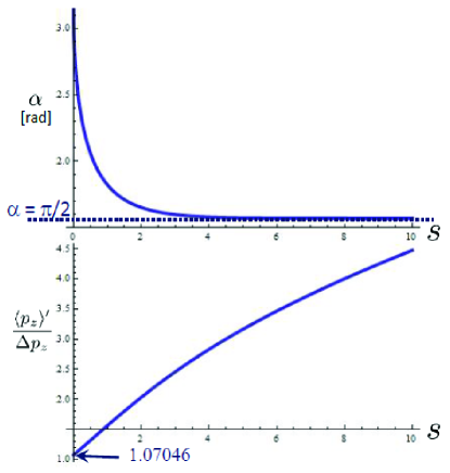
Figure 5: The optimal SNR line (upper panel) (58) on the $(s,\alpha)$-plane and the optimally pre-selected SNR (59) (lower panel) are shown. The optimally pre-selected SNR is a monotonically increasing function of $s$. In the strong-measurement regime $s\gg 1$, this SNR increases due to the fact that pre-selected state $\alpha=\pi/2$ is the eigenstate $|\uparrow_{z}\rangle$ of the operator $\sigma_{z}$. In the weak-measurement regime $s\ll 1$, the SNR cannot be larger than that in the strong-measurement regime but has the minimum value $\langle p_{z}\rangle^{\prime}/\Delta p_{z}\sim 1.07046$.

As shown in Fig. 5, in the strong-measurement regime $s\gg 1$, this SNR increases due to the fact that pre-selected state $\alpha=\pi/2$ is the eigenstate $|\uparrow_{z}\rangle$ of the operator $\sigma_{z}$. On the other hand, in the weak-measurement regime $s\ll 1$, the SNR cannot be larger than that in the strong-measurement regime but has the minimum value on the optimal SNR line. Actually, for $s\ll 1$, the asymptotic expansion of Eq. (59) yields

$$\frac{\langle p_{z}\rangle^{\prime}}{\Delta p_{z}} = \sqrt{\frac{2}{\sqrt{3}}}+\frac{1}{3}\sqrt{1+\frac{2}{\sqrt{3}}}s+O(s^{2}),$$ (60)

which is larger than $\sqrt{2/\sqrt{3}}\sim 1.0746$.

V Application to the simplified DSJH setup

In this section, we apply our formulae, which are summarized in Sec. III.1, to the simplified DSJH P.B.Dixon-D.J.Starling-A.N.Jordan-J.C.Howell-2009 setup. We discuss the optimization of the expectation value of transverse deflections of an optical beam in Sec. V.3 and the optimization of the SNR in Sec. V.4.

V.1 Simplified setup of experiment

The simplified version of the DSJH experiment is the measurement of the tiny tilt of the piezo-driven mirror in a Sagnac interferometer P.B.Dixon-D.J.Starling-A.N.Jordan-J.C.Howell-2009 . In Ref. P.B.Dixon-D.J.Starling-A.N.Jordan-J.C.Howell-2009 , they use the which-path information of a photon in the Sagnac interferometer, which is represented by the photon states $|\circlearrowright\rangle$ and $|\circlearrowleft\rangle$. Here, $|\circlearrowright\rangle$ ($|\circlearrowleft\rangle$) is the state of a photon which propagates along the clockwise (counter-clockwise) direction in the Sagnac interferometer. As the pre-selected state $|\psi_{i}\rangle$ of a photon, they choose

$$|\psi_{i}\rangle=\frac{1}{\sqrt{2}}\left(ie^{i\phi/2}|\circlearrowleft\rangle+e^{-i\phi/2}|\circlearrowright\rangle\right),$$ (61)

where $\phi$ is the phase difference of the states $|\circlearrowright\rangle$ and $|\circlearrowleft\rangle$ introduced by a Soleil-Babinet compensator.

The weak interaction in the weak measurement is described by the interaction Hamiltonian

$${\cal H}=kx\otimes{\bf A}\delta(t-t_{0}),$$ (62)

where $k$ is the momentum shift of the light path by the tilt of the piezo-driven mirror and $x$ represents the shift of the light image at the dark port of the interferometer. The quantum operator ${\bf A}$ in Eq. (62) is given by

$${\bf A}=|\circlearrowright\rangle\langle\circlearrowright|-|\circlearrowleft\rangle\langle\circlearrowleft|.$$ (63)

We note that the operator ${\bf A}$ satisfy the property ${\bf A}^{2}=1$. Then, we may apply our formulae given in Sec. III.

As the post-selection of a photon state, we choose the dark-port in the Sagnac interferometer

$$|\psi_{f}\rangle=\frac{1}{\sqrt{2}}\left(|\circlearrowleft\rangle+i|\circlearrowright\rangle\right),$$ (64)

and the weak value in this setup is given by

$$\langle{\bf A}\rangle_{w}=\frac{\langle\psi_{f}|{\bf A}|\psi_{i}\rangle}{\langle\psi_{f}|\psi_{i}\rangle}=-i\cot\frac{\phi}{2}.$$ (65)

where $\phi$ is the pre-selection angle in Eq. (61). We note that this weak value (65) is pure imaginary.

Comparing Eq. (62) with Eq. (1), we find the correspondence of variables as

$$p\rightarrow x,\quad q\rightarrow-p,\quad g\rightarrow k,$$ (66)

where new variables $x$ and $p$ satisfy the commutation relation $[x,p]=i$.

Although Dixon et al. modified the beam radius of the laser by lenses in Ref. P.B.Dixon-D.J.Starling-A.N.Jordan-J.C.Howell-2009 , we do not take account of the effect of this modification. This modification is not essential to the basic mechanism of the weak measurement. This is the reason why we call the “simplified” DSJH setup in this paper.

V.2 All-order expectation values and probability distribution

Here, we apply the formulae summarized in Sec. III.1 to the above simplified DSJH setup.

The normalization factor ${\cal Z}$ [Eq. (19)], is given by

$${\cal Z} = \frac{1-e^{-s}\cos\phi}{1-\cos\phi},$$ (67)

where $s$ is the coupling parameter [see Eq. (20)] defined by

$$s:=2k^{2}\langle x^{2}\rangle.$$ (68)

The expectation values of $x$ and $p$ after the post-selection are given by

$$k\langle x\rangle^{\prime}=-\frac{se^{-s}\sin\phi}{1-e^{-s}\cos\phi},\quad\langle p\rangle^{\prime}=0.$$ (69)

Fluctuations $\Delta x:=\sqrt{\langle(x-\langle x\rangle^{\prime})^{2}\rangle^{\prime}}$ and $\Delta p:=\sqrt{\langle(p-\langle p\rangle^{\prime})^{2}\rangle^{\prime}}$ in $x$ and $p$ are given by

$$k^{2}(\Delta x)^{2} = \frac{s}{2}+\frac{s^{2}e^{-s}\left(\cos\phi-e^{-s}\right)}{\left(1-e^{-s}\cos\phi\right)^{2}},$$ (70)

$$\frac{1}{k^{2}}(\Delta p)^{2} = \frac{1}{2s}+\frac{1}{1-e^{-s}\cos\phi}.$$ (71)

As in the case of AAV setup, the first term in Eq. (70) [Eq. (71)] shows the initial variance in $x$ (in $p$). The remaining terms in Eqs. (70) and (71) are due to the pre-selection, weak interaction, and the post-selection.

In Fig. 6, the expectation value $-k\langle x\rangle^{\prime}$ of Eq. (69) is shown as a function of the coupling parameter $s=2k^{2}\langle x^{2}\rangle^{\prime}$ and the pre-selection angle $\phi$.

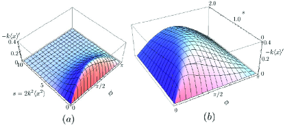
Figure 6: $-k\langle x\rangle^{\prime}$ [Eq. (69)] is shown as a function of the coupling $s=2k^{2}\langle x^{2}\rangle$ and the pre-selection angle $\phi$ in two ranges of $s$. (a) $s\in(0,10)$, (b) $s\in(0,2)$. For large $s$, the expectation value $-k\langle x\rangle^{\prime}$ decays exponentially. From these figures, we can see that, for a given coupling parameter $s$, there is a pre-selection angle $\phi$ such that the expectation value of $x$ is maximized.

In the simplified DSJH setup, the probability density in $x$-space is obtained from Eq. (25) as

$$\langle x|\rho_{d}^{\prime}|x\rangle = \frac{1-\cos(2kx-\phi)}{1-e^{-s}\cos\phi}\langle x|\rho_{d}|x\rangle,$$ (72)

where $\langle x|\rho_{d}|x\rangle$ is the initial probability density in $x$-space:

$$\langle x|\rho_{d}|x\rangle=\frac{k}{\sqrt{\pi s}}\exp\left[-\frac{k^{2}x^{2}}{s}\right].$$ (73)

V.3 Expectation value optimization

Here, we consider the optimization of the expectation value amplification in the simplified DSJH setup. From Fig. 6, we can see that the expectation value (69) exponentially decays in the strong measurement regime $s\gg 1$ (Fig. 6(a)). Furthermore, Fig. 6(b) also shows that, for a given coupling parameter $s$, there is a pre-selection angle $\phi$ such that the expectation value of $x$ is maximized. This is the optimal expectation value of $-k\langle x\rangle^{\prime}$ for a fixed coupling parameter $s$. To seek this optimal expectation value, we consider the equation $\partial(-k\langle x\rangle^{\prime})/\partial\phi=0$, which yields the equation

$$\cos\phi=e^{-s}.$$ (74)

This is the equation for the optimal expectation-value line on $(\phi,s)$-plane. On this optimal line, the expectation-value of $x$ and the fluctuation $\Delta x$ in $x$ are given by

$$k\langle x\rangle^{\prime} = -\frac{se^{-s}}{\sqrt{1-e^{-2s}}}=:k\langle x\rangle^{\prime}_{\mbox{opt}},$$ (75)

$$k\Delta x = \sqrt{\frac{s}{2}}.$$ (76)

We note that the variance [Eq. (76)] in $x$ after the optimal post-selection coincides with that of the initial state of the detector. The optimal expectation-value line (74) and the expectation value of $-k\langle x\rangle^{\prime}$ (75) on this optimal line is shown in Fig. 7.

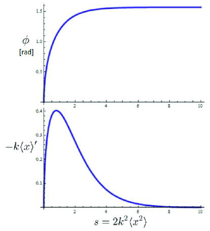
Figure 7: The optimal expectation-value line (74) (upper panel) and the expectation value of $-k\langle x\rangle^{\prime}$ (75) (lower panel) on this optimal line is shown as a function of the coupling parameter $s$. In the limit $s\rightarrow\infty$, the optimal pre-selection angle for expectation value approaches to $\phi\rightarrow\pi/2$. Further, on the optimal expectation-value line, the expectation value $-k\langle x\rangle^{\prime}$ has the maximum value at $s\sim 0.8$.

From Eq. (72), the probability density on the optimal expectation-value line (74) is given by

$$\langle x|\rho_{d}^{\prime}|x\rangle = \frac{1-e^{-s}\cos(2kx)-\sqrt{1-e^{-2s}}\sin(2kx)}{1-e^{-2s}}$$ (77)

$$\quad\quad\quad\times\frac{k}{\sqrt{\pi s}}\exp\left[-\frac{k^{2}x^{2}}{s}\right],$$

which is shown in Fig. 8. The $s=0.1$ case, which corresponds to the weak measurement on the optimal expectation-value line (74), shows that the peak of the probability distribution slightly deviates from the linear result $s\Im A_{w}$ given in Ref. P.B.Dixon-D.J.Starling-A.N.Jordan-J.C.Howell-2009 , and that the probability density after the post-selection is slightly different from the Gaussian distribution. When the coupling parameter $s$ is large, many peaks appear in the probability density in $x$-space and the expectation value $\langle x\rangle^{\prime}$ after the post-selection approaches to zero due to the contribution of these many peaks.

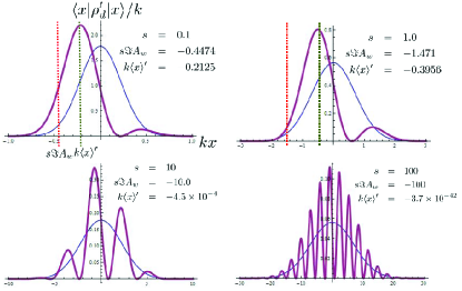
Figure 8: [Online Color] Probability distribution functions (77) in $x$-space on the optimal expectation-value line (74) with some coupling parameters $s$ are shown by the thick line (red line). We also plot the initial probability distribution $\langle x|\rho_{d}\rangle/k$ in Eq. (73) with the same coupling parameter $s$ by the thin lines (blue lines). The $s=0.1$ case corresponds to the weak measurement on the optimal expectation-value line (74). This shows that the peak of the probability distribution slightly deviates from the linear result $s\Im A_{w}$. The $s=1.0$ case is still essentially same as $s=0.1$ case. The maximal expectation value ($s=s_{m}\sim 0.8$) is obtained around this parameter. The $s=10$ and $s=1000$ cases correspond to the strong measurement case.

In the limit $s\rightarrow\infty$, the optimal expectation-value line approaches to $\phi\rightarrow\pi/2$. Further, we have to note that, on the optimal expectation-value line, the expectation value $-k\langle x\rangle^{\prime}$ has the maximum value at $s\sim 0.8$. This is maximal value of $-k\langle x\rangle^{\prime}$ on whole $(\phi,s)$-plane. To seek this maximum point, we consider the equation $\partial(k\langle x\rangle^{\prime}_{\mbox{opt}})/\partial s=0$. The solution $s=s_{m}$ to this equation is derived from the equation

$$1-s_{m}-e^{-2s_{m}}=0.$$ (78)

The numerical value of $s_{m}$ is $s_{m}\simeq 0.79681$. Therefore, the expectation value satisfy the inequality

$$-k\langle x\rangle^{\prime}\leq\left.-k\langle x\rangle^{\prime}_{opt}\right|_{s=s_{m}}\simeq 0.402371.$$ (79)

At this maximum point, the optimal pre-selection angle $\phi_{m}$ is determined by $\cos\phi_{m}=e^{-s_{m}}$, which yields $\phi_{m}\simeq 1.103$ rad $\simeq 63.2^{\circ}$. We also note that the expectation value $\langle x\rangle^{\prime}$ at the maximum point $s=s_{m}$ itself is proportional to $k^{-1}$. Therefore, we can obtain the large expectation value $\langle x\rangle^{\prime}$ if we have a small coupling constant $k$ in the interaction Hamiltonian (62).

If we evaluate the amplification factor ${\cal A}$ by following to the discussion by Dixon et al. P.B.Dixon-D.J.Starling-A.N.Jordan-J.C.Howell-2009 , the amplification factor is given by ${\cal A}=|\langle x\rangle^{\prime}|/\delta$. Here, $\delta=kl_{md}/k_{0}$ is the unamplified deflection without the interferometer. The unamplified deflection in their experiment is $\delta\sim 3$ $\mu$m. On the other hand, from Eq. (79), we obtain $|\langle x\rangle^{\prime}_{opt}|_{s=s_{m}}|\simeq 0.4/k$ at the maximum point $s=s_{m}$. Since $k\sim 2\times 10^{-5}$ $\mu$m^-1 in their experiment, the maximal amplification is estimated as ${\cal A}_{max}\sim 600$.

However, since the definition of $s$ is given by Eq. (68) and the fluctuation $\sqrt{\langle x^{2}\rangle}$ of the initial variance is regarded as the beam radius, $s_{m}\sim 0.8$ corresponds to $\sqrt{\langle x^{2}\rangle}\sim 0.63\times(1/k)$. The optimal beam radius in their setup is given by $\sqrt{\langle x^{2}\rangle}\sim 3$ cm from Eq. (79). On the other hand, the maximum expectation value $-\langle x\rangle^{\prime}\sim 0.4\times(1/k)\sim 2$ cm. For one-photon case, the SNR at the maximal point $s=s_{m}$ is given by $|\langle x\rangle^{\prime}|/\Delta x\sim 0.6$, which is independent of the coupling constant $k$ in the interaction Hamiltonian. For this reason, in Sec. V.4, we consider the optimization of this SNR.

V.4 SNR optimization

As in the case of the AAV setup, we consider the optimization of the SNR. From Eqs. (69) and (70), the SNR is given by

$$\frac{\left|\langle x\rangle^{\prime}\right|}{\Delta x}=\frac{\sqrt{2s}e^{-s}\sin\phi}{\sqrt{\left(1-e^{-s}\cos\phi\right)^{2}+2se^{-s}\left(\cos\phi-e^{-s}\right)}}.$$

(80)

The behavior of this SNR on $(\phi,s)$-plane is shown in Fig. 9, which indicates that the SNR (80) in the simplified DSJH setup is maximized only in the weak measurement regime $s<1$.

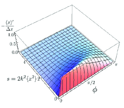
Figure 9: The signal to noise ratio (SNR) (80) in simplified DSJH setup are shown as a function of the coupling parameter $s$ and the pre-selection angle $\phi$. This shows that the SNR in this setup have the peak only in the weak measurement regime $s<1$.

To carry out the optimization of the SNR (80), we consider the equation $\partial(|\langle x\rangle^{\prime}|/\Delta x)/\partial\phi=0$, which yields

$$\cos^{2}\phi+2\frac{(\cosh s-se^{-s})}{s-1}\cos\phi+1=0.$$ (81)

The solution $\phi=\phi_{\mbox{opt}}$ to Eq. (81) is given by

$$\cos\phi_{\mbox{opt}}(s) := -\frac{\cosh s-se^{-s}}{s-1}$$

$$+\frac{\sqrt{(\cosh s-se^{-s})^{2}-(s-1)^{2}}}{s-1},$$

Equation (LABEL:eq:Dixon-et-al-2009-kouchan-62-a) describes the optimal line on $(\phi,s)$-plane. On this optimal line, the optimal SNR is given by

$$\left.\frac{\left|\langle x\rangle^{\prime}\right|}{\Delta x}\right|_{\mbox{opt}}:=\left.\frac{\left|\langle x\rangle^{\prime}\right|}{\Delta x}\right|_{\phi=\phi_{\mbox{opt}}}.$$ (83)

Along the optimal line [Eq. (LABEL:eq:Dixon-et-al-2009-kouchan-62-a)], the optimized SNR is shown in Fig. 10. The optimal SNR (83) is a monotonically decreasing function of $s$. Further, only in the region $s<0.15$, the optimal SNR (83) can be larger than unity. Actually, for $s\ll 1$, the asymptotic behavior of the optimal SNR (83) is given by

$$\left.\frac{\left|\langle x\rangle^{\prime}\right|}{\Delta x}\right|_{\mbox{opt}} = \sqrt{\frac{2}{\sqrt{3}}}-\frac{1}{3}\sqrt{1+\frac{2}{\sqrt{3}}}s+O(s^{2})$$ (84)

$$< \sqrt{\frac{2}{\sqrt{3}}},$$

where $\sqrt{2/\sqrt{3}}\simeq 1.0746$. Thus, we have shown that the upper limit of the SNR in the simplified DSJH setup for the single photon case is of the order of unity.

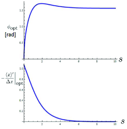
Figure 10: The optimal-SNR pre-selection angle $\phi_{\mbox{opt}}$ [the solution to Eq. (LABEL:eq:Dixon-et-al-2009-kouchan-62-a)] (upper panel) and the optimized SNR (83) (lower panel) in simplified DSJH setup are shown as a function of the coupling parameter $s$. This shows that the SNR in this setup have the peak only in the weak measurement regime $s<1$. The maximum SNR is of the order of unity in the single photon case.

VI Summary

In summary, after reviewing the formulation by Wu and Li S.Wu-Y.Li-2010 , we derived some formulae for the weak measurement of the operator ${\bf A}$ which satisfies the property ${\bf A}^{2}=1$ through their formulation. We have to emphasize that our formulae are based on the exact evaluation of the formulation of Wu and Li. In the derivation of these formulae, we assume that the initial state of the detector is zero mean-value Gaussian. We note that we do not use any additional condition to derive these formulae. Our formulae are valid not only in the weak measurement regime but also in the strong measurement regime. Due to this fact, we could clarify the connection between the strong measurement regime and the weak measurement regime.

We applied our formulae to two experimental setups. One is the experiment of the weak measurement using spin-1/2 particles, which was proposed in AAV original paper of the weak measurement Y.Aharonov-D.Z.Albert-L.Vaidman-1988 . The other is the simplified version of the optical experiment in the Sagnac interferometer (simplified DSJH setup) by Dixon et al. P.B.Dixon-D.J.Starling-A.N.Jordan-J.C.Howell-2009 . These two experimental setups are typical experiments of the weak measurements. The weak value is real in the AAV setup, while it is pure imaginary in the simplified DSJH setup. In these setups, we have two control parameters. One is the pre-selection angles in these experiment and the other is the coupling parameter $s$ defined by Eq. (20). We discussed the behavior of the expectation values of the detector variables in the whole range of these two parameters.

In both setups of AAV and DSJH, we found that for a fixed coupling parameter $s$, there exits the pre-selection (or post-selection) which maximize the expectation values of variables for the detector or the SNR. The precise estimation of this optimal pre-selection (or post-selection) is possible through the exact expression of the expectation values summarized in this paper. This is the main results of this paper. The existence of this optimal pre-selection (or post-selection) comes from the fact that we specify the subensemble of system through the post-selection in weak measurements. Since the post-selection is the restriction of the system ensemble, the density matrix of the detector after the postselection is renormalized by this restriction. This is the essential reason of the appearance of the normalization factor ${\cal Z}$ in Eq. (9). The behavior of the normalization factor ${\cal Z}$ leads the existence of this optimal pre-selection (or post-selection).

Furthermore, we showed that the optimized SNR is order of unity in the weak measurement regime for the single particle (or photon) experiment in both experimental setups. To improve this SNR, we have to consider the large $N$ ensemble of particles (or photons). Due to this large $N$ ensemble, the SNR is improved by the factor $\sqrt{N}$ as proposed by Aharonov and Vaidman Aharonov-Vaidman-2007-update-review . In particular, the photon number is very large in the experiments using the laser beam (for example, the experiment by Dixon et al. P.B.Dixon-D.J.Starling-A.N.Jordan-J.C.Howell-2009 ). For this reason, the large SNR should be obtained in the actual experiments.

Finally, we have to emphasize that many other experiments are also categorized into the case of ${\bf A}^{2}=1$ and the initial Gaussian state of the detector. For example, the experiment by Iinuma et al. M.Iinuma-Y.Suzuki-G.Taguchi-Y.Kadoya-H.F.Hofmann-2011 corresponds to the experiment to measure the operator ${\bf A}$, which satisfies ${\bf A}^{2}=1$, with a real weak value. They experimentally confirmed the formula (21). The experiment by Hosten and Kwiat O.Hosten-P.Kwiat-2008 corresponds to the experiment of the operator ${\bf A}$, which satisfies ${\bf A}^{2}=1$, with a weak value of pure imaginary. Thus, we may say that there are many experiments to which our formulae are applicable. Of course, in some actual experiments, there are some complexity which we did not take into account in this paper. For example, the modification of the beam radius by lenses in DSJH experiment P.B.Dixon-D.J.Starling-A.N.Jordan-J.C.Howell-2009 was not included in our treatment. Furthermore, we might have to care about the validity of the von-Neumann interaction model (41) in real experiments. Although there are some issues to be taken into account when we apply our arguments to specific experiments, we expect that our exact expressions of some expectation values in a weak measurement will be useful to understand experimental results or to propose some new experimental setups.

Appendix A Derivations of formulae

In this appendix, we show the derivations of the formulae summarized in Sec. III. Our derivation use the Wu-Li formulation S.Wu-Y.Li-2010 reviewed in Sec. II. Since their formulation requires the separate treatments according to the norm of the pre- and post-selected states, we first consider, in Sec. A.1, the non-orthogonal case in which the pre- and post-selection is not orthogonal. Then, in Sec. A.2, we consider the case where the pre- and post-selected states is orthogonal.

A.1 Non-orthogonal case

When the norm $\left|\langle\psi_{f}|\psi_{i}\rangle\right|$ is non-vanishing, the density matrix after the post-selection is given by Eq. (LABEL:eq:detector-density-matrix-after-PS). Only through the property ${\bf A}^{2}=1$, the normalization factor ${\cal Z}$ and the density matrix $\rho_{d}^{\prime}$, which are given by Eqs. (9) and (LABEL:eq:detector-density-matrix-after-PS), are reduced to the following series

$${\cal Z} = 1+\frac{1}{2}\sum_{n=1}^{+\infty}\frac{(-i2g)^{2n}}{(2n)!}\langle p^{2n}\rangle\left(1-\left|\langle{\bf A}\rangle_{w}\right|^{2}\right)+i\sum_{n=0}^{+\infty}\frac{(-i2g)^{2n+1}}{(2n+1)!}\langle p^{2n+1}\rangle\Im\langle{\bf A}\rangle_{w},$$ (85)

$$\rho_{d}^{\prime} = {\cal Z}^{-1}\left[\rho_{d}+\sum_{n=1}^{+\infty}\frac{(-ig)^{2n}}{(2n)!}\left(\sum_{k=0}^{n}{}_{2n}C_{2k}p^{2n-2k}\rho_{d}p^{2k}-\left|\langle{\bf A}\rangle_{w}\right|^{2}\sum_{k=0}^{n-1}{}_{2n}C_{2k+1}p^{2n-2k-1}\rho_{d}p^{2k+1}\right)\right.$$ (86)

$$\quad\quad\quad\left.+\sum_{n=0}^{+\infty}\frac{(-ig)^{2n+1}}{(2n+1)!}\left(\langle{\bf A}\rangle_{w}\sum_{k=0}^{n}{}_{2n+1}C_{2k}p^{2n+1-2k}\rho_{d}p^{2k}-\langle{\bf A}\rangle_{w}^{*}\sum_{k=0}^{n}{}_{2n+1}C_{2k+1}p^{2n-2k}\rho_{d}p^{2k+1}\right)\right].$$

From this density matrix (86), we can evaluate the expectation values of $p$, $q$, $p^{2}$, and $q^{2}$ after the post-selection as follows

$${\cal Z}\langle p\rangle^{\prime} = \langle p\rangle+\frac{1}{2}\left(1-\left|\langle{\bf A}\rangle_{w}\right|^{2}\right)\sum_{n=1}^{+\infty}\frac{(-i2g)^{2n}}{(2n)!}\langle p^{2n+1}\rangle+i\Im\langle{\bf A}\rangle_{w}\sum_{n=0}^{+\infty}\frac{(-i2g)^{2n+1}}{(2n+1)!}\langle p^{2n+2}\rangle,$$ (87)

$${\cal Z}\langle q\rangle^{\prime} = \langle q\rangle+g\left(\Re\langle{\bf A}\rangle_{w}+\Im\langle{\bf A}\rangle_{w}\langle(qp+pq)\rangle\right)+\frac{1}{2}i\Im\langle{\bf A}\rangle_{w}\sum_{n=1}^{+\infty}\frac{(-i2g)^{2n+1}}{(2n+1)!}\langle qp^{2n+1}+p^{2n+1}q\rangle$$ (88)

$$+\frac{1}{4}\left(1-\left|\langle{\bf A}\rangle_{w}\right|^{2}\right)\sum_{n=1}^{+\infty}\frac{(-4g^{2})^{n}}{(2n)!}\langle qp^{2n}+p^{2n}q\rangle,$$

$${\cal Z}\langle p^{2}\rangle^{\prime} = \langle p^{2}\rangle+\frac{1}{2}\left(1-\left|\langle{\bf A}\rangle_{w}\right|^{2}\right)\left(\sum_{n=1}^{+\infty}\frac{(-i2g)^{2n}}{(2n)!}\langle p^{2n+2}\rangle\right)+i\Im\langle{\bf A}\rangle_{w}\left(\sum_{n=0}^{+\infty}\frac{(-i2g)^{2n+1}}{(2n+1)!}\langle p^{2n+3}\rangle\right),$$ (89)

$${\cal Z}\langle q^{2}\rangle^{\prime} = \langle q^{2}\rangle+g\left(2\Re\langle{\bf A}\rangle_{w}\langle q\rangle+\Im\langle{\bf A}\rangle_{w}\langle q^{2}p+pq^{2}\rangle\right)+\frac{g^{2}}{2}\left(2\left|\langle{\bf A}\rangle_{w}\right|^{2}-\left(1-\left|\langle{\bf A}\rangle_{w}\right|^{2}\right)\langle q^{2}p^{2}+p^{2}q^{2}\rangle\right)$$ (90)

$$+\frac{1}{2^{2}}\left(1-\left|\langle{\bf A}\rangle_{w}\right|^{2}\right)\sum_{n=2}^{+\infty}\frac{(-i2g)^{2n}}{(2n)!}\left(\langle q^{2}p^{2n}+p^{2n}q^{2}\rangle+\frac{1}{2}(2n)(2n-1)\langle p^{2n-2}\rangle\right)$$

$$+\frac{i}{2}\Im\langle{\bf A}\rangle_{w}\sum_{n=1}^{+\infty}\frac{(-2ig)^{2n+1}}{(2n+1)!}\left(\langle q^{2}p^{2n+1}+p^{2n+1}q^{2}\rangle+\frac{1}{2}(2n+1)(2n)\langle p^{2n-1}\rangle\right)$$

where $\langle*\rangle^{\prime}:={{\mbox{Tr}}}_{d}\left(*\rho_{d}^{\prime}\right)$. Further, the probability densities $\langle p|\rho_{d}^{\prime}|p\rangle$ in $p$-space and $\langle q|\rho_{d}^{\prime}|q\rangle$ in $q$-space are given by

$${\cal Z}\langle p|\rho_{d}^{\prime}|p\rangle = \left[1+\frac{1}{2}\left(1-\left|\langle{\bf A}\rangle_{w}\right|^{2}\right)\left(\cos(2gp)-1\right)+\Im\langle{\bf A}\rangle_{w}\sin(2gp)\right]\langle p|\rho_{d}|p\rangle,$$ (91)

$${\cal Z}\langle q|\rho_{d}^{\prime}|q\rangle = \left|\langle q|\phi\rangle\right|^{2}+{\cal I}+{\cal J},$$ (92)

where ${\cal I}$ and ${\cal J}$ are defined by

$${\cal I} := \sum_{n=1}^{+\infty}\frac{g^{2n}}{(2n)!}\left\{\sum_{k=0}^{n}{}_{2n}C_{2k}\left(\frac{\partial^{2n-2k}}{\partial q^{2n-2k}}\langle q|\phi\rangle\right)\left(\frac{\partial^{2k}}{\partial q^{2k}}\langle q|\phi\rangle\right)^{*}\right.$$ (93)

$$\quad\quad\quad\quad\quad\quad\quad\quad\quad\quad\left.+\left|\langle{\bf A}\rangle_{w}\right|^{2}\sum_{k=0}^{n-1}{}_{2n}C_{2k+1}\left(\frac{\partial^{2n-2k-1}}{\partial q^{2n-2k-1}}\langle q|\phi\rangle\right)\left(\frac{\partial^{2k+1}}{\partial q^{2k+1}}\langle q|\phi\rangle\right)^{*}\right\},$$

$${\cal J} := -\sum_{n=0}^{+\infty}\frac{g^{2n+1}}{(2n+1)!}\left\{\langle{\bf A}\rangle_{w}\sum_{k=0}^{n}{}_{2n+1}C_{2k}\left(\frac{\partial^{2n+1-2k}}{\partial q^{2n+1-2k}}\langle q|\phi\rangle\right)\left(\frac{\partial^{2k}}{\partial q^{2k}}\langle q|\phi\rangle\right)^{*}\right.$$ (94)

$$\quad\quad\quad\quad\quad\quad\quad\quad\left.+\langle{\bf A}\rangle_{w}^{*}\sum_{k=0}^{n}{}_{2n+1}C_{2k+1}\left(\frac{\partial^{2n-2k}}{\partial q^{2n-2k}}\langle q|\phi\rangle\right)\left(\frac{\partial^{2k+1}}{\partial q^{2k+1}}\langle q|\phi\rangle\right)^{*}\right\}.$$

When the initial state of the detector is zero-mean value Gaussian (17), the moments of $p$ are given by Eqs. (18). In this case, the normalization ${\cal Z}$ [Eq. (85)] is given by Eq. (19). Similar calculations with the properties

$$\langle(qp^{n}+p^{n}q)\rangle = 0\quad\mbox{for}\quad n\geq 1,$$ (95)

$$\langle q^{2}p^{2n}+p^{2n}q^{2}\rangle = -\frac{2n-1}{2}\frac{(2n-1)!!}{(2a)^{n-1}},$$ (96)

$$\langle q^{2}p+pq^{2}\rangle = \langle q^{2}p^{2n+1}+p^{2n+1}q^{2}\rangle$$ (97)

$$= 0,\quad\mbox{for}\quad n\geq 1$$

of the zero mean-value Gaussian state lead to the expectation values of $p$ and $q$ [Eq. (21) and (22)] after the post-selection and the variances in $p$ and $q$ [Eq. (23) and (24)] after the post-selection. We also note that the derivation of the probability density (25) in $p$-space is straight forward, while the derivation of Eq. (26) is non-trivial. Therefore, we only explain the derivation Eq. (26).

The initial state $\langle q|\phi\rangle$ of the detector is derived from the Fourier transformation of Eq. (17):

$$\langle q|\phi\rangle = \left(\frac{s}{\pi g^{2}}\right)^{1/4}\exp\left[-\frac{s}{2}\left(\frac{q}{g}\right)^{2}\right].$$ (98)

From the definition of the Hermite polynomial I.S.Gradshteyn-I.M.Ryzhik-2000 :

$$H_{n}(x):=(-1)^{n}e^{x^{2}/2}\frac{d^{n}}{dx^{n}}(e^{-x^{2}/2}),$$ (99)

we easily obtain

$$\frac{\partial^{n}}{\partial q^{n}}\langle q|\phi\rangle=(-g)^{-n}s^{n/2}H_{n}\left(\frac{\sqrt{s}q}{g}\right)\langle q|\phi\rangle.$$ (100)

This formula (100) is used to evaluate the derivative of the initial wave function (98) in Eqs. (93) and (94).

To evaluate $\langle q|\rho_{d}^{\prime}|q\rangle$ through Eq. (92), we first consider the second term ${\cal I}$ in Eq. (92):

$${\cal I} = \langle q|\rho_{d}|q\rangle\sum_{n=1}^{+\infty}\frac{s^{n}}{(2n)!}\left\{\sum_{k=0}^{n}{}_{2n}C_{2k}H_{2n-2k}\left(\frac{\sqrt{s}q}{g}\right)H_{2k}\left(\frac{\sqrt{s}q}{g}\right)\right.$$ (101)

$$\quad\quad\quad\quad\quad\quad\quad\quad\quad\quad\left.+\left|\langle{\bf A}\rangle_{w}\right|^{2}\sum_{k=0}^{n-1}{}_{2n}C_{2k+1}H_{2n-2k-1}\left(\frac{\sqrt{s}q}{g}\right)H_{2k+1}\left(\frac{\sqrt{s}q}{g}\right)\right\}$$

Here, we note that the Hermite polynomial (99) is an even function of $x$ if the index $n$ is even and an odd function of $x$ if the index $n$ is odd I.S.Gradshteyn-I.M.Ryzhik-2000 , i.e.,

$$H_{2n}(-x)=H_{2n}(x),$$ (102)

$$H_{2n+1}(-x)=-H_{2n+1}(x),$$ (103)

$$H_{2k}(0)=(-1)^{k}(2k-1)!!,\;\;H_{2k+1}(0)=0.$$ (104)

Further, we also note the sum rule of the Hermite polynomial I.S.Gradshteyn-I.M.Ryzhik-2000 :

$$H_{n}(x+y)=\frac{1}{2^{n/2}}\sum_{r=0}^{n}{}_{n}C_{r}H_{n-r}(\sqrt{2}x)H_{r}(\sqrt{2}y).$$

(105)

Through these formulae (102)–(105), we easily obtain

$$\sum_{r=0}^{k}{}_{2k}C_{2r}H_{2k-2r}(\sqrt{2}x)H_{2r}(\sqrt{2}x)$$

$$= 2^{k-1}\left(H_{2k}(2x)+(-1)^{k}(2k-1)!!\right),$$

$$\sum_{r=0}^{k-1}{}_{2k}C_{2r+1}H_{2k-2r-1}(\sqrt{2}x)H_{2r+1}(\sqrt{2}x)$$

$$= 2^{k-1}\left(H_{2k}(2x)-(-1)^{k}(2k-1)!!\right),$$

$$\sum_{r=0}^{k}{}_{2k+1}C_{2r}H_{2k+1-2r}(\sqrt{2}x)H_{2r}(\sqrt{2}x)$$

$$= 2^{k-1/2}H_{2k+1}(2x),$$

$$\sum_{r=0}^{k}{}_{2k+1}C_{2r+1}H_{2k-2r}(\sqrt{2}x)H_{2r+1}(\sqrt{2}x)$$

$$= 2^{k-1/2}H_{2k+1}(2x).$$ (109)

Through the formulae (A.1)–(109), Eq. (101) is given by

$${\cal I} = \frac{1}{2}\left|\langle q|\phi\rangle\right|^{2}\left[\sum_{n=0}^{+\infty}\frac{(2s)^{n}}{(2n)!}H_{2n}\left(\frac{\sqrt{2s}q}{g}\right)\right.$$

$$\quad\quad\quad\quad\quad\left.+\left(1-\left|\langle{\bf A}\rangle_{w}\right|^{2}\right)e^{-s}-2\right.$$

$$\quad\quad\quad\quad\quad\left.+\left|\langle{\bf A}\rangle_{w}\right|^{2}\left(\sum_{n=0}^{+\infty}\frac{(2s)^{n}}{(2n)!}H_{2n}\left(\frac{\sqrt{2s}q}{g}\right)\right)\right].$$

Here, we note the formulae I.S.Gradshteyn-I.M.Ryzhik-2000 :

$$\sinh(tx) = e^{t^{2}/2}\sum_{n=0}^{\infty}H_{2n+1}(x)\frac{t^{2n+1}}{(2n+1)!},$$ (111)

$$\cosh(tx) = e^{t^{2}/2}\sum_{n=0}^{\infty}H_{2n}(x)\frac{t^{2n}}{(2n)!}.$$ (112)

Through the formula (112),

$${\cal I} = \left|\langle q|\phi\rangle\right|^{2}e^{-s}\left[\cosh^{2}\left(\frac{sq}{g}\right)-e^{s}\right.$$ (113)

$$\quad\quad\quad\quad\quad\quad\left.+\left|\langle{\bf A}\rangle_{w}\right|^{2}\sinh^{2}\left(\frac{sq}{g}\right)\right].$$

Using Eq. (111), the similar evaluation of the final term ${\cal J}$ in Eq. (92) yields

$${\cal J} = \left|\langle q|\phi\rangle\right|^{2}\Re\langle{\bf A}\rangle_{w}e^{-s}\sinh\left(\frac{2sq}{g}\right).$$ (114)

Through Eqs. (113) and (114), we can evaluate Eq. (92) and the probability density in $q$-space is given by Eq. (26) with the initial probability density in $q$-space (28).

A.2 Orthogonal case

In the orthogonal weak measurements $\langle\psi_{f}|\psi_{i}\rangle=0$, the orthogonal weak value is trivial as shown in Eq. (31). Through the orthogonal weak value (31), the normalization constant ${\cal Z}_{o}$ defined by Eq. (LABEL:eq:S.Wu-Y.Li-2010-22) is given by

$${\cal Z}_{o} = 1+2\sum_{n=1}^{+\infty}\frac{(-4g^{2})^{n}}{(2n+2)!}\frac{\langle p^{2n+2}\rangle}{\langle p^{2}\rangle}.$$ (115)

The density matrix of the detector after the post-selection is given by Eq. (33).

The expectation value of $p$, $q$, $p^{2}$, and $q^{2}$ after the post-selection are evaluated as

$${\cal Z}_{o}\langle p^{2}\rangle\langle p\rangle^{\prime} = {\cal Z}_{o}\langle p^{2}\rangle{{\mbox{Tr}}}\left(p\rho_{d}^{\prime}\right)$$ (116)

$$= \langle p^{3}\rangle+2\sum_{n=1}^{+\infty}\frac{(-i2g)^{2n}}{(2n+2)!}\langle p^{2n+3}\rangle,$$

$${\cal Z}_{o}\langle p^{2}\rangle\langle q\rangle^{\prime} = {\cal Z}_{o}\langle p^{2}\rangle{{\mbox{Tr}}}\left(q\rho_{d}^{\prime}\right)$$ (117)

$$= \frac{1}{2}\langle qp^{2}+p^{2}q\rangle$$

$$+\sum_{n=1}^{+\infty}\frac{(-i2g)^{2n}}{(2n+2)!}$$

$$\quad\quad\times\langle qp^{2n+2}+p^{2n+2}q\rangle,$$

$${\cal Z}_{o}\langle p^{2}\rangle\langle p^{2}\rangle^{\prime} = {\cal Z}_{o}\langle p^{2}\rangle{{\mbox{Tr}}}\left(p^{2}\rho_{d}^{\prime}\right)$$ (118)

$$= \langle p^{4}\rangle+2\sum_{n=1}^{+\infty}\frac{(-4g^{2})^{n}}{(2n+2)!}\langle p^{2n+4}\rangle,$$

$${\cal Z}_{o}\langle p^{2}\rangle\langle q^{2}\rangle^{\prime} = {\cal Z}_{o}\langle p^{2}\rangle{{\mbox{Tr}}}\left[q^{2}\rho_{d}^{\prime}\right]$$ (119)

$$= 1+\frac{1}{2}\langle q^{2}p^{2}+p^{2}q^{2}\rangle$$

$$+\frac{1}{2}\sum_{n=1}^{+\infty}\frac{(-4g^{2})^{n}}{(2n+2)!}\left(2\langle q^{2}p^{2n+2}+p^{2n+2}q^{2}\rangle\right.$$

$$\quad\quad\quad\left.+(2n+2)(2n+1)\langle p^{2n}\rangle\right).$$

From the density matrix (33), we can directly obtain the probability density in $p$-space as

$$\langle p|\rho_{d}^{\prime}|p\rangle=\frac{1}{{\cal Z}_{o}\langle p^{2}\rangle}\frac{1}{4g^{2}}\left(1-\cos(2gp)\right)\langle p|\rho_{d}|p\rangle.$$ (120)

On the other hand, we also obtain the probability density in $q$-space as

$${\cal Z}_{o}\langle p^{2}\rangle\langle q|\rho_{d}^{\prime}|q\rangle = \langle q|p\rho_{d}p|q\rangle+\sum_{n=1}^{+\infty}\frac{(-ig)^{2n}}{(2n+2)!}\sum_{k=0}^{n}{}_{2n+2}C_{2k+1}\langle q|p^{2(n-k)+1}\rho_{d}p^{2k+1}|q\rangle.$$ (121)

since we choose the initial state of the detector as a pure state $\rho_{d}=|\phi\rangle\langle\phi|$, Eq. (121) yields

$$\langle q|\rho_{d}^{\prime}|q\rangle = \frac{1}{{\cal Z}_{o}\langle p^{2}\rangle}\left[\left(\frac{\partial}{\partial q}\langle q|\phi\rangle\right)\left(\frac{\partial}{\partial q}\langle q|\phi\rangle\right)^{*}\right.$$ (122)

$$\quad\quad\quad\quad\left.+\sum_{n=1}^{+\infty}\frac{g^{2n}}{(2n+2)!}\sum_{k=0}^{n}{}_{2n+2}C_{2k+1}\left(\frac{\partial^{2(n-k)+1}}{\partial q^{2(n-k)+1}}\langle q|\phi\rangle\right)\left(\frac{\partial^{2k+1}}{\partial q^{2k+1}}\langle q|\phi\rangle\right)^{*}\right].$$

When the initial state of the detector is Gaussian (17), we use Eqs. (18) and (95)–(97). Then, the expectation values of $p$ and $q$ after the post-selection are trivial as shown in Eqs. (34) and (35). Since the expectation values of $p$ and $q$ after the post-selection vanish, the expectation values of $p^{2}$ and $q^{2}$ themselves represent the variances in $p$ and $q$ after the post-selection. Then we obtain Eqs. (36) and (37). Furthermore, the probability density (120) in $p$-space trivially yields Eq. (38). However, the expression of the probability density (39) in $q$-space requires the non-trivial derivation from Eq. (122). Therefore, we briefly explain the derivation of Eq. (39) below.

Since our initial state of the detector is a zero mean-value Gaussian (98), we also apply the formula (100). Substituting Eq. (100) into Eq. (122), we obtain

$${\cal Z}_{o}\langle p^{2}\rangle\langle q|\rho_{d}^{\prime}|q\rangle = \left|\langle q|\phi\rangle\right|^{2}\frac{s^{2}q^{2}}{g^{4}}$$ (123)

$$+\left|\langle q|\phi\rangle\right|^{2}\frac{s}{g^{2}}\sum_{n=1}^{+\infty}\frac{s^{n}}{(2n+2)!}\sum_{k=0}^{n}{}_{2n+2}C_{2k+1}H_{2n-2k+1}\left(\frac{\sqrt{s}q}{g}\right)H_{2k+1}\left(\frac{\sqrt{s}q}{g}\right).$$

Through formulae (112) and (A.1), the calculations similar to the derivation (26) yields (39).

References

- (1) Y. Aharonov, D. Z. Albert, and L. Vaidman, Phys. Rev. Lett. 60 (1988), 1351.
- (2) Y. Aharonov, A. Botero, S. Pospescu, B. Reznik, and J. Tollaksen, Phys. Lett. A 301 (2002), 130; J. S. Lundeen and A. M. Steinberg, Phys. Rev. Lett. 102 (2009), 020404; K. Yokota, T. Yamamoto, M. Koashi, and N. Imoto, New J. Phys. 11 (2009), 033011.
- (3) N. W. M. Ritchie, J. G. Story, and R. G. Hulet, Phys. Rev. Lett. 66 (1991), 1107.
- (4) G. J. Pryde, J. L. O’Brien, A. G. White, T. C. Ralph, H. M. Wiseman, Phys. Rev. Lett. 94 (2005), 220405.
- (5) O. Hosten and P. Kwiat, Science 319 (2008), 787; K.J.Resch, Science 319 (2008), 733.
- (6) P. B. Dixon, D. J. Starling, A. N. Jordan, and J. C. Howell, Phys. Rev. Lett. 102 (2009), 173601; J. C. Howell, D. J. Starling, P. B. Dixon, P. K. Vudyasetu, and A. N. Jordan, Phys. Rev. A 81 (2010), 033813.
- (7) D. J. Starling, P. B. Dixon, A. N. Jordan, and J. C. Howell, Phys. Rev. A 80 (2009), 041803(R).
- (8) M. Iinuma, Y. Suzuki, G. Taguchi, Y. Kadoya, and H. F. Hofmann, New J. Phys. 13 (2011), 033041.
- (9) J. von Neumann: Mathematical Foundations of Quantum Mechanics (Princeton Univ. Press, Princeton, NJ, 1955).
- (10) Y. Aharonov and L. Vaidman, Lec. Notes Phys. 734 (2008), 399; and reference therein.
- (11) Y. Aharonov and A. Botero, Phys. Rev. A 72 (2005), 052111.
- (12) A. Di Lorenzo and J. C. Egues, Phys. Rev. A 77 (2008), 042108.
- (13) S. Wu and Y. Li, Phys. Rev. A 83 (2011), 052106. [arXiv:1010.1155v1[quant-ph]].
- (14) R. Jozsa, Phys. Rev. A 76 (2007), 044103.
- (15) I.M. Duck, P. M. Stevenson, and E. C. G. Sudarshan, Phys. Rev. D40 (1989), 2112.
- (16) I. S. Gradshteyn and I. M. Ryzhik, “Table of Integrals, Series, and Products Sixth Edition”, (Edited by A. Jeffrey and D. Zwillinger, Translated from the Russian by Scripta Technica, Inc., Academic Press, 2000)