The molecular distribution of the IRDC $\rm{G}351.77-0.51$

Abstract

Context. Infrared dark clouds are massive, dense clouds seen in extinction against the IR Galactic background. Many of these objects appear to be on the verge of star and star cluster formation.

Aims. Our aim is to understand the physical properties of IRDCs in very early evolutionary phases. We selected the filamentary IRDC $\rm{G}351.77-0.51$, which is remarkably IR quiet at 8$\mu$m.

Methods. As a first step, we observed mm dust continuum emission and rotational lines of moderate and dense gas tracers to characterise different condensations along the IRDC and study the velocity field of the filament.

Results. Our initial study confirms coherent velocity distribution along the infrared dark cloud ruling out any coincidental projection effects. Excellent correlation between MIR extinction, mm continuum emission and gas distribution is found. Large-scale turbulence and line profiles throughout the filament is indicative of a shock in this cloud. Excellent correlation between line width, and MIR brightness indicates turbulence driven by local star formation.

1 Introduction

Although the majority of stars, especially massive stars, are observed to form in clusters (Testi et al., 1997, 1999; Lada & Lada, 2003; de Wit et al., 2004), our understanding of star formation is mainly based on studies of nearby star-forming regions that mostly give birth to isolated low-mass stars. On the other hand, little is known about the formation of clusters and of stars in clusters. Naturally, studies of clusters should begin by understanding their youngest evolutionary phases. However, the youngest (proto)clusters would still be deeply embedded within their natal dense clouds, thus obscured from view except at far IR/millimetre wavelengths. Due to the coarse angular resolution of millimetre observations, studies of deeply embedded (proto)clusters have so far focused on the nearest star forming regions in Ophiuchus (Motte et al., 1998; Johnstone et al., 2004; André et al., 2007), Perseus (Johnstone et al., 2010) and Serpens (Testi & Sargent, 1998; Testi et al., 2000; Olmi & Testi, 2002). These regions, however, do not form massive stars and rich clusters and it is therefore necessary to extend these studies to more distant massive star-forming regions. Observational studies of the initial conditions for the formation of massive clusters have so far been very limited (e.g. Molinari et al., 1998, 2002; Beuther & Schilke, 2004) but will soon find a new renaissance with the high angular resolution and sensitivity offered by the Atacama Large Millimeter/submillimeter Array (ALMA).

Infrared dark clouds (IRDCs) are ideal candidates for studying the earliest phases of the formation of clusters. They were discovered as dark patches in the sky at IR wavelengths against the bright Galactic background during mid-IR imaging surveys with the Infrared Space Observatory (ISO, Perault et al., 1996) and the Mid-course Space Experiment (MSX, Egan et al., 1998). Their spatial coincidence with emission from molecular lines and dust indicates that they consist of dense molecular gas and dust of a few $10^{5}$ cm^-3 density (Carey et al., 1998, 2000). Temperatures in these clouds are low enough (10–20 K, Pillai et al., 2006a) that they do not radiate significantly even at mid-IR wavelengths: of the 190 dust cores in IRDCs surveyed by Rathborne et al. (2010) only 93 have detectable emission at 24$\mu$m.

The formation mechanism of IRDC is still a matter of debate (Myers, 2009). Recent results (e.g., Jiménez-Serra et al., 2010; Hernandez & Tan, 2011) may support models of filament formation from converging flows. However, there is still no solid conclusion about their origin. Tan (2007) suggests that IRDC may contain the sites of future massive star and star cluster formation, since their densities and mass surface densities are similar to regions known to be undergoing such formation activity. Indeed, emerging evidence suggests that the earliest phases of the formation of high-mass star and cluster are occurring within these clouds (e.g., Pillai et al., 2006b; Rathborne et al., 2006). Studies of IRDCs have often focused on sources that already have intense star formation activity and are therefore in late protostellar evolutionary phases (e.g., Pillai et al., 2006b; Rathborne et al., 2008). However, to address questions related to the formation of clusters, and of the single stars in them, studies of earlier evolutionary phases with no or modest star formation are needed.

The IRDC under investigation in this paper is at Galactic coordinates $(l,b)$=$(351^{\circ}.77,-00^{\circ}.51)$, and was identified by Simon et al. (2006) in the 8$\mu$m data from the MSX satellite as $\rm{G}351.77-0.51$ (hereafter G351.77). G351.77 appears as a filament of dust, which is seen in absorption against the mid-IR background of our Galaxy (see Fig. 1) up to 24$\mu$m (Carey et al., 2009) and in emission in the millimetre range (Faúndez et al., 2004). Following Motte et al. (2007), we used the 8$\mu$m MSX image as a starting point to infer the stellar activity of the filament. G351.77 is remarkably quiet at this wavelength: emission is detected towards five positions in the filament, three of them being close to the bright IR source IRAS 17233$-$3606. Compact emission is detected in more sensitive Spitzer images towards other positions in the filament (see Sect. 3). IRAS 17233$-$3606 lies near one end of the filament. This source shows several signs of active massive star formation: different authors (Caswell et al., 1980; Fix et al., 1982; Menten, 1991) detected very intense H₂O, OH, and CH₃OH masers, while Leurini et al. (2008, 2009) report the discovery of bipolar outflows originating in the vicinity of IRAS 17233$-$3606 and a molecular spectrum typical of hot molecular cores near massive young stellar objects. If IRAS 17233$-$3606 is part of the molecular environment of G351.77, the distance of G351.77 would be relatively close, since studies of IRAS 17233$-$3606 locate it at $D\leq 1$ kpc (see Leurini et al., 2011, and reference therein). The near distance would imply that high linear resolution observations could be performed even with single-dish radio telescopes whose typical angular resolutions are not better than $10\arcsec$, corresponding to 0.05 pc at 1 kpc. In addition, given its low declination, G351.77 would be an ideal candidate for high angular resolution observations with ALMA to study the earliest stages of formation of massive stars and stellar cluster, and to investigate the content of low- and intermediate-mass star formation in IRDCs.

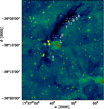
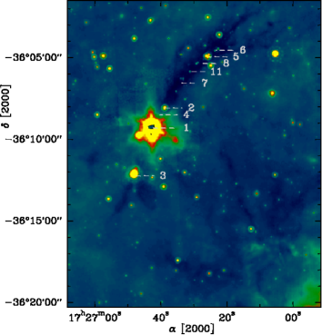
Figure 1: Image of the 8$\mu$m (left) and 24$\mu$m (right) emission from Spitzer of the molecular cloud $\rm{G}351.77-0.51$. The numbers label the 870$\mu$m dust continuum clumps found by the CLUMPFIND procedure and discussed in the text (see Table 3).

2 Observations

2.1 APEX observations

The Large Apex BOlomoter CAmera (LABOCA, Siringo et al., 2009) was used to observe the continuum emission at 870$\mu$m towards the dust filament G351.77. The FWHM beam size of APEX at 870$\mu$m is $\sim 19\aas@@fstack{\prime\prime}2$. The data are part of the ATLASGAL survey of the Galactic plane (Schuller et al., 2009). Observations were done with fast-scanning, linear, on-the-fly maps in total-power mode (i.e. without chopping secondary). Details on the data reduction are given in Schuller et al. (2009). In particular, the subtraction of correlated skynoise results in a filtering of uniform extended emission on scales larger than $\sim$2.5^′; compact or filamentary sources should not be strongly affected, though. For a detailed discussion of filtering of extended structures, we refer to Belloche et al. (2011). The calibration of the LABOCA data relies on opacity correction based on skydips and on observations of planets as primary calibrators and of well-known, bright, compact sources as secondary calibrators. As a result, the photometric uncertainty is of the order of 10%.

Table 1: Summary of the parameters of the APEX and MOPRA line observations.

Setup	Tuning Frequency	Telescope	Beam	$\Delta\rm{v}$
	(MHz)		($\arcsec$)	(km s-1)
N2H+ (1–0)	93173.5	MOPRA	$35\aas@@fstack{\prime\prime}0$	0.1
13CO-C18O (2–1)	219980.0	APEX	$28\aas@@fstack{\prime\prime}4$	0.17
C17O (2–1)	224700.0	APEX	$27\aas@@fstack{\prime\prime}8$	0.16

Observations in ¹³CO, C¹⁸O and C¹⁷O $(2-1)$ towards selected positions in G351.77 were performed during the science verification programme (project number 081.F-9805(A)) of the APEX-1 receiver on APEX in 2008 June (19 and 25) and August (21, 30 and 31). The observations in June were performed under mediocre weather conditions (with 2–3 mm precipitable water vapour), yielding system temperatures of 240-400 K. The observations in August were, on the other hand, performed under excellent atmospheric transmissions (down to 0.4 mm precipitable water vapour), yielding system temperatures of 160-210 K. The observed transitions and basic observational parameters are summarised in Table 1.

For the observations, we used the APEX facility FFT spectrometer (Klein et al., 2006). The ¹³CO and C¹⁸O $(2-1)$ transitions were covered in one frequency setup, with the APEX-1 receiver tuned to 219.98 GHz in the lower side band. A second frequency setup was used to cover the C¹⁷O $(2-1)$ line, with the APEX-1 receiver tuned to 224.7 GHz in the lower side band. For both setups, we performed long integration observations on selected positions (Table 2). For the ¹³CO–C¹⁸O setup, we observed an additional strip of five points (($20\arcsec$,$-20\arcsec$), ($10\arcsec$,$-10\arcsec$), ($0\arcsec$,$0\arcsec$), ($-10\arcsec$,$10\arcsec$), and ($-20\arcsec$,$20\arcsec$)), centred on the position G351.62 of Table 2. For both frequency setups, data were taken in the position-switching mode, with a reference position $(600\arcsec,0\arcsec)$ in horizontal coordinates from the targets.

We used a main-beam efficiency of 0.75 to convert antenna temperatures into main-beam temperatures. A detailed description of APEX and of its performance is given by Güsten et al. (2006).

Table 2: Positions observed with APEX

Position	R.A. [J2000]	Dec. [J2000]	Setup
Clump-1a	17:26:42.30	-36:09:18.23	13CO-C18O, C17O
Clump-2	17:26:38.79	-36:08:05.53	13CO-C18O, C17O
Clump-3	17:26:47.33	-36:12:14.37	13CO-C18O, C17O
Clump-4	17:26:40.30	-36:08:29.63	13CO-C18O
Clump-5	17:26:25.25	-36:04:57.03	13CO-C18O, C17O
Clump-6	17:26:23.25	-36:04:32.74	13CO-C18O
Clump-7	17:26:34.78	-36:06:34.22	13CO-C18O, C17O
Clump-8	17:26:28.26	-36:05:21.34	13CO-C18O
Clump-9b	17:25:31.96	-36:22:15.70	13CO-C18O, C17O
Clump-10c	17:26:06.66	-36:22:09.63	13CO-C18O, C17O
Clump-12b	17:25:31.97	-36:21:21.05	13CO-C18O
G351.62	17:26:34.80	-36:17:41.00	13CO-C18O

• IRAS 17233–3606

• Clump-9 and 12 are offset from IRAS 17221–3619

• IRAS 17227–3619

2.2 MOPRA observations

The observations were carried out with the ATNF Mopra telescope on 2007 June 30 under clear sky conditions. Two adjacent fields were observed in $220\times 220$ arcsec² on-the-fly maps for 30 minutes each. The HEMT receiver was tuned to 92.2 GHz and the MOPS spectrometer was used in narrow band mode to cover the 8 GHz bandwidth of the receiver with about 0.1 km/s velocity resolution. The beam size at these frequencies is about 35 arcsec. The system temperature was 175 K. Pointing was checked and corrected with line pointings on the SiO maser source AH Sco.

Initial processing of the data was done using the ATNF tools livedata and gridzilla and included the subtraction of the off signal, the calibration to T${}_{a}^{*}$ units, the baseline subtraction and the gridding. To convert antenna to main beam brightness temperature, we corrected the data for an antenna efficiency of 0.5. Details on antenna efficiency in the 3mm band is given by Ladd et al. (2005). The data was then exported to MIRIAD and GILDAS for further processing.

3 IR emission

Figures 1 and 1 show G351.77 at 8 and 24$\mu$m, respectively, from the GLIMSPE and MIPSGAL surveys of the Galactic plane (Benjamin et al., 2003; Carey et al., 2009). The filament is dark at both wavelengths except for bright emission associated with IRAS 17233–3606 (dust condensation 1, hereafter clump 1) and with the dust condensation 3 (clump 3) to the south of IRAS 17233–3606 (see Table 3). Additionally, weak emission, which is still compact in most of the cases, is detected at several positions along the filament at both wavelengths. Compact emission at 24$\mu$m is an indicator of active star formation, since this emission traces warm dust heated as material accretes from a core onto a central protostar. To search for evidence of outflow activity from young stellar objects, we also checked the 4.5$\mu$m map of the region made with the Spitzer InfraRed Array Camera (IRAC). Extended green emission (4.5$\mu$m) is clearly associated only with the outflows originating in IRAS 17233–3606 (Leurini et al., 2009). A jet-like feature extends from IRAS 17233–3606 into the dark filament. More compact emission at 4.5$\mu$m is also detected towards three additional positions in G351.77 (clumps 2, 3, and 5).

A larger map of the region in the IRAC 8$\mu$m image reveals a complex picture: extended emission along a semicircular structure is detected opposite to G351.77. Moreover, the map is dominated by the infrared source IRAS 17221–3619, which is associated with bubble CS84 of the catalogue of Churchwell et al. (2007), and belongs to a second circular structure seen in emission in the mid-IR (Fig. 3). Several dark patches are seen at 8$\mu$m and 24$\mu$m, two of them being the IRDCs $\rm{G}351.62-0.58$ and $\rm{G}351.77-0.60$ (see Fig. 3 and Table 2) identified in the catalogue of Simon et al. (2006).

4 Continuum emission at 870$\mu$m

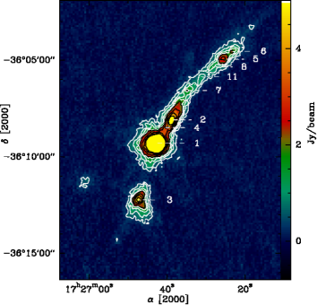
Figure 2: LABOCA map of the 870$\mu$m dust continuum emission from the IRDC G351.77–0.51. The white contours are from 5$\sigma$ (0.425 Jy/beam) to 2 Jy/beam in steps of 5$\sigma$; the black contours are from 2  Jy/beam to 5 Jy/beam in steps of 10$\sigma$. The numbers label the clumps found by the CLUMPFIND procedure and discussed in the text (see Table 3).

The continuum emission at 870$\mu$m probes cold dust. Therefore, it can be used to locate dense compact clumps, potential sites of star and cluster formation. Given the linear resolution of our LABOCA map ($19\aas@@fstack{\prime\prime}2\sim 0.1$ pc at 1 kpc), our data are sensitive to dust clumps possibly associated with cluster formation (Williams et al., 2000; Testi et al., 2000; Olmi & Testi, 2002).

Our LABOCA map of $\rm{G}351.77$ reveals extended continuum dust emission that matches the morphology of the mid-IR extinction extremely well (Figs. 2 and 3). The IRDC $\rm{G}351.77-0.60$ coincides with the $6\sigma$ LABOCA emission on the east of IRAS 17233–3606 (Fig. 3). On larger scales, the emission extends over a curved structure (Fig. 3), which includes the IRDC $\rm{G}351.62-0.58$ (see previous section) associated with our position G351.62, and the sources IRAS 17227–3619 and IRAS 17221–3619 (see Table 2). A second, intense peak of continuum emission is found opposite to IRAS 17233–3606, on its west. This emission is, however, associated with the IR source IRAS 17220–3609, whose molecular lines have a velocity of $-98.5$ km s^-1 (Bronfman et al., 1996), which implies a kinematic distance of 10 kpc (Faúndez et al., 2004). Since IRAS 17233–3606 has a velocity of $-3.4$ km s^-1, the two sources are unlikely to be physically related. We conclude that IRAS 17220–3609 is projected close to the line of sight of IRAS 17233–3606, but it is much further away from the Sun, so we did not include IRAS 17220–3609 in our following analysis.

No continuum emission at 870$\mu$m is associated with the semicircular structure opposite to G351.77 seen at 8$\mu$m (Fig. 3), hence probably due to low density gas not sampled by our observations. Since our molecular line follow-up observations were only performed toward peaks of emission at 870$\mu$m, we do not have any information on the velocity field of this structure and we cannot determine whether it is physically associated with G351.77 or not.

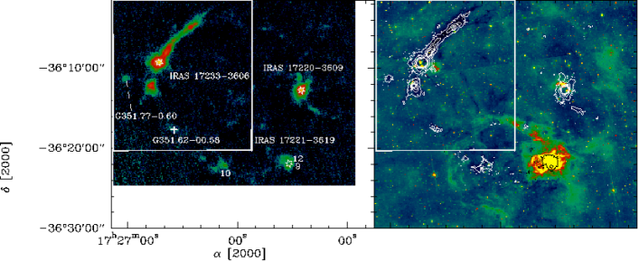
Figure 3: Left: Continuum emission at 870$\mu$m of the environment around $\rm{G}351.77-0.51$. The numbers label the clumps found by the CLUMPFIND algorithm outside the region plotted in Fig. 1. The white cross marks the position G351.62, the stars the IRAS sources found in the region. Right: Image of the emission at 8$\mu$m of the molecular environment around $\rm{G}351.77-0.51$. The white (and black for IRAS 17221–3619) contours show the emission at 870$\mu$m from 0.255 (3 $\sigma$) to 4 Jy/beam in step of 10 $\sigma$. In both panels, the white box outlines the region plotted in Fig. 1.

4.1 Identification of the clumps

Table 3: Results of the CLUMPFIND calculations

Clump	$S_{\nu}$	$F_{\nu}$	$\theta_{x}^{\mathrm{a}}$	$\theta_{y}^{\mathrm{a}}$	$\theta^{\mathrm{b}}$	IRc
	[Jy]	[Jy/beam]	[$\arcsec$]	[$\arcsec$]	[$\arcsec$]
$\rm{G}351.77-0.51$
1	159.4	54.2	43.6	38.5	41.1	$8,24\mu$m
2	29.7	6.2	31.6	46.7	39.3	$8,24\mu$m
3	24.9	5.2	31.5	49.6	40.7	$8,24\mu$md
4	16.1	4.0	46.9	25.2	36.5	e
5	9.3	3.1	18.8	20.9	19.8	$8,24\mu$m
6	6.1	2.3	21.5	19.3	20.4	$24\mu$m
7	8.7	2.1	33.0	41.5	37.3
8	4.6	1.5	17.5	20.5	19.1	$24\mu$m
11	3.2	1.1	20.6	22.7	21.7	$8,24\mu$m
other positions
9	4.8	1.5	28.9	21.1	25.1	$8,24\mu$m
10	2.7	1.2	23.1	12.4	18.2	$8,24\mu$m
12	5.0	1.0	46.9	21.5	34.8	$8,24\mu$m

• deconvolved ${{\it FWHM}_{x}}$ and ${{\it FWHM}_{y}}$

• deconvolved geometric mean of ${{\it FWHM}_{x}}$ and ${{\it FWHM}_{y}}$

• association with IR emission

• the IR source is offset from the mm source

• position contaminated by the emission from IRAS 17233–3606

To identify clumps in the millimetre continuum emission and define their properties, we used a two-dimensional variation of the clump-finding algorithm CLUMPFIND developed by Williams et al. (1994). The algorithm works by effectively contouring the data at a multiple of the rms noise of the map, then searching for peaks of emission to locate the clumps, and finally following the clump profile down to lower intensities. The advantage of this method is that it does not a priori assume any shape for the clumps. However, since the contouring levels are chosen by hand, the algorithm does not take any emission into account below the user-selected threshold. Recently, Pineda et al. (2009) have outlined some weaknesses of the method, which may lead to erroneous mass functions for crowded regions. Nevertheless, the CLUMPFIND algorithm may still be useful for studying the structure of one cloud as in our case. We set the threshold level to 5$\sigma$.

The procedure calculates the peak position, the full width at half maximum not corrected for beam size for the x-axis, ${{\it FWHM}_{x}}$, and for the y-axis, ${{\it FWHM}_{y}}$, and the total flux density integrated within the clump boundary within the threshold level.

We identified twelve clumps in the 870$\mu$m continuum emission over the region shown in Fig. 3. The centroid coordinates delivered by CLUMPFIND are given in Table 2. Other results of the CLUMPFIND analysis are given in Table 3 where we also indicate whether clumps are associated with continuum emission at 8 and 24$\mu$m, either point-like or diffuse. We interpret the detection of a compact 24$\mu$m source in all clumps of G351.77 except clumps 4 and 7 as a confirmation of the validity of the method used for identifying clumps in the region. While clump 7 is clearly detected as a secondary peak of emission at 870$\mu$m, clump 4 does not look like a clumpy structure at visual inspection, and could be an example of ’pathological’ features created by CLUMPFIND in case of significant emission found between prominent clumps (see Goodman et al., 2009). Additionally, we note that clump 1 is associated with the active massive star-forming region IRAS 17233–3606 discussed above, and that clumps 9 and 12 are associated with the infrared source IRAS 17221–3619, which hosts an Hii region (e.g., Martín-Hernández et al., 2003) surrounding an IR star cluster candidate (Borissova et al., 2006) associated with bubble CS84.

Table 4: Physical parameters of the clumps derived from the LABOCA emission.

Clump	$M_{\rm{10K}}$	$M_{\rm{25K}}$	$M_{\rm{35K}}$	$N_{{\rm{H}_{2}},{\rm 10K}}$	$N_{{\rm{H}_{2}},{\rm{25K}}}$	$N_{{\rm{H}_{2}},{\rm 35K}}$	$n_{{\rm{H}_{2}},{\rm 10K}}$	$n_{{\rm{H}_{2}},{\rm{25K}}}$	$n_{{\rm{H}_{2}},{\rm 35K}}$
	[$M_{\odot}$]	[$M_{\odot}$]	[$M_{\odot}$]	[$10^{22}$ cm-2]	[$10^{22}$ cm-2]	[$10^{22}$ cm-2]	[$10^{5}$ cm-3]	[$10^{5}$ cm-3]	[$10^{5}$ cm-3]
$\rm{G}351.77-0.51$
1	2964	664	428	460	103	66	108	24	16
2	552	124	80	52	12	8	23	5	3
3	463	104	67	44	10	6	17	4	3
4	300	67	43	34	8	5	16	3	2
5	173	39	25	27	6	4	56	13	8
6	113	25	16	19	4	3	34	7	5
7	161	36	23	18	4	3	8	2	1
8	85	19	12	13	3	2	31	7	4
11	60	13	9	10	2	1	15	3	2
other positions
9	89	20	13	13	3	2	14	3	2
10	51	11	7	10	2	1	21	5	3
12	94	21	14	9	2	1	6	1	1

4.2 Mass estimate

The masses of the clumps given in Table 4 are derived by assuming that the continuum emission at 870$\mu$m is optically thin:

$$M_{tot}=\frac{d^{2}F_{\nu}}{\kappa_{\nu}B_{\nu}(T_{d})}$$ (1)

where $F_{\nu}$ is the integrated flux, $d$ the distance of the source, $\kappa$ the dust opacity, and $B(T_{d})$ is the Planck function for a black body of dust temperature $T_{d}$, all for a frequency of $\sim 340$ GHz. For the dust opacity, we adopted a value of 0.0182 cm² g^-1 (from Table 1, Col. 5 of Ossenkopf & Henning, 1994). This agrees with recent measurements of dust opacities at 850 and 450$\mu$m from Shirley et al. (2011) in the low-mass Class 0 core B335.

From the line observations performed towards the dust filament of G351.77, we confirm that IRAS 17233–3606 belongs to the same molecular environment of the infrared dark cloud G351.77 (see Sect. 5). We assume a distance of 1 kpc in the following calculations. Our mass estimates would be a factor of 2 smaller for a distance of 700 pc (see Sect. 1), corresponding to the smallest distance of IRAS 17233–3606 reported in the literature (Miettinen et al., 2006). We also computed beam-averaged H₂ volume densities assuming that the clumps have spherical symmetry and a mean molecular weight per hydrogen molecule, $\mu_{\rm H_{2}}$, of 2.8 (see discussion in Kauffmann et al. 2008). From previous line observations, we know that clump 1 (IRAS 17233–3606) harbours a hot core (Leurini et al., 2008), while our current data towards the other clumps do not reveal any rich molecular spectrum indicative of hot core activity, i.e., an embedded central heating source. Ammonia (1,1) and (2,2) observations with the Parkes telescope (Wienen et al. in prep.) of three positions along the filament (clump 1, 2, and 3) infer temperatures of $<$20 K on an angular size of $\sim 1\arcmin$. Except for clump 1, which hosts the hot core associated with IRAS 17233–3606, we believe that temperatures of 10–25 K are appropriate for the dust in the clumps in G351.77 where only point-like emission is detected at 24$\mu$m. We computed masses, column densities, and densities of all clumps also for $T_{d}=35$ K for consistency with Sect. 5.2. Results can be easily scaled to higher temperatures: compared to the values given for $T_{d}=35$ K, estimates are a factor $\sim 1.5$ smaller for $T_{d}=50$ K, likely to be an upper limit to the temperature of the dust for IRAS 17233–3606 at the resolution of the data. For $T=25$ K, the lowest mass derived from our analysis for the clumps in G3512.77 is 13 $M_{\odot}$ (clump 11), while all other clumps have masses of several tens of solar masses. As a result, G351.77 has the potential of forming intermediate to high-mass stars or clusters of low-mass stars in several positions along the filament.

5 Emission from CO isotopologues

5.1 Velocity field

To derive the velocity of each clump, we used the optically thin C¹⁷O $(2-1)$ line (see Sect. 5.2). The C¹⁸O $(2-1)$ transition was used for the positions that are not observed in C¹⁷O (see Table 2). Both transitions were detected towards all positions towards which they were observed. To derive the parameters of the C¹⁷O line, we used the HFS method in CLASS. A Gaussian fit was applied to the C¹⁸O and ¹³CO $(2-1)$ lines, although their spectra show more complex velocity structures. The ¹³CO line often shows evidence of non-Gaussian wings and multiple peaks. These are probably due to self absorption, as the optical thinner C¹⁸O and C¹⁷O transitions peak at the velocity of the dip in the ¹³CO spectrum. Negative features at other velocities are most likely due to emission in the reference positions used during the observations. However, in the clumps that were observed in all three isotopologues, no absorption feature is detected in the C¹⁷O spectrum. Therefore we believe that our results (based on the analysis of the C¹⁷O spectra, see Sect. 6.1) are not affected by this problem. The spectra of all clumps are shown in Figs. 4 and 5, while the results of the fit are listed in Table 5.

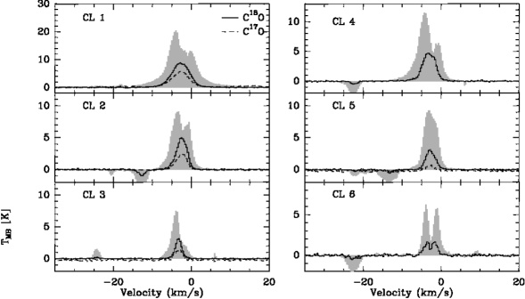
Figure 4: In grey, spectra of ¹³CO (2–1) of clumps 1, 2, 3, 4, 5 and 6. The solid and dashed spectra are C¹⁸O (2–1), and C¹⁷O (2–1) respectively.

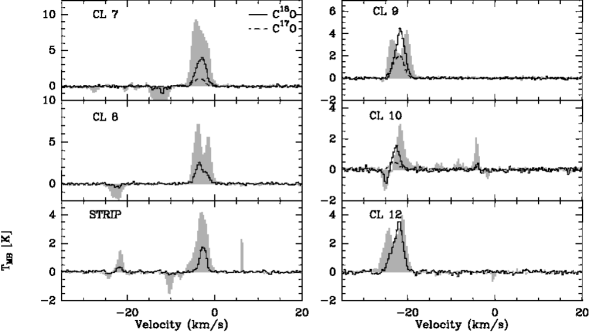
Figure 5: In grey, spectra of ¹³CO (2–1) of clumps 7, 8, 9, 10, 12 and position G351.62. The solid and dashed spectra are C¹⁸O (2–1), and C¹⁷O (2–1) respectively.

From the analysis of the velocity field, we found two different molecular components along the ring of dust detected at $870\leavevmode\nobreak\ \mu$m, and all clumps along the infrared dark cloud G351.77 are at velocities $-3$ km s^-1, including clump 3, immediately south of IRAS 17233–3606 (clump 1). We confirm the $5\sigma$ dust continuum detection at the position G351.62 $(\alpha_{2000}=17^{h}26^{m}34^{s}.80,\delta_{2000}=-36^{\circ}17^{\prime}41\aas@@fstack{\prime\prime}00)$ to be due to dense material, since both ¹³CO $(2-1)$ and C¹⁸O $(2-1)$ are detected at that position, with a velocity similar to that of G351.77. Clumps 9 and 12 (see Fig. 3) have velocities around $-22$ km s^-1. Moreover, at three positions (clump 3, clump 10, and G351.62) two velocity components are detected in emission, in ¹³ CO $(2-1)$ at clumps 3 and 10, and in ¹³ CO $(2-1$) and C¹⁸O $(2-1)$ at all five points across the position G351.62. The two velocity components (clump 3: $-3.2$ and $-24.5$ km s^-1; clump 10: $\sim-4.0$ and $-21.5$ km s^-1; G351.62: $-2.6$ and $-21.9$ km s^-1) belong to the same molecular environment of the infrared dark cloud G351.77 and to that of clumps 9 and 12. On clump 4, the feature at $\rm{v}_{LSR}-3.2$ km s^-1 shows non-Gaussian blue-shifted wings; on clump 10, the feature at $-21.5$ km s^-1 also has non Gaussian red-shifted wings.

Table 5: Line parameters of the C¹⁷O and C¹⁸O$(2-1)$ transitions. The symbol – means that the line was not observed.

Clump	$\rm{v}_{\rm LSR}$	$\Delta\rm{v}$	$\int T_{\rm mb}\delta\rm{v}$a	$\rm{v}_{\rm LSR}$	$\Delta\rm{v}$	$\int T_{\rm mb}\delta\rm{v}$
	[km s-1]	[km s-1]	[K km s-1]	[km s-1]	[km s-1]	[K km s-1]
	C17O			C18O
1b	$-2.51\pm 0.04$	$5.0\pm 0.1$	$32.1\pm 0.5$	$-2.65\pm 0.02$	$5.68\pm 0.04$	$84.0\pm 0.5$
2	$-2.21\pm 0.02$	$2.4\pm 0.1$	$8.4\pm 0.1$	$-2.28\pm 0.02$	$3.33\pm 0.06$	$21.3\pm 0.3$
3	$-2.95\pm 0.06$	$1.4\pm 0.2$	$4.2\pm 0.2$	$-3.16\pm 0.02$	$2.17\pm 0.05$	$10.1\pm 0.2$
4	–	–	–	$-3.16\pm 0.02$	$3.66\pm 0.06$	$20.8\pm 0.3$
5	$-2.6\pm 0.1$	$2.2\pm 0.3$	$2.3\pm 0.2$	$-2.66\pm 0.03$	$2.82\pm 0.07$	$11.7\pm 0.3$
6c	–	–	–	$-2.5\pm 0.1$	$4.0\pm 0.3$	$6.9\pm 0.4$
7	$-3.35\pm 0.03$	$1.9\pm 0.2$	$3.52\pm 0.07$	$-3.19\pm 0.05$	$2.6\pm 0.1$	$12.1\pm 0.4$
8d	–	–	–	$-3.39\pm 0.05$	$2.5\pm 0.1$	$6.8\pm 0.3$
9	$-21.80\pm 0.02$	$1.94\pm 0.09$	$6.33\pm 0.08$	$-21.70\pm 0.02$	$2.43\pm 0.05$	$14.9\pm 0.3$
10	$-22.80\pm 0.07$	$2.1\pm 0.2$	$1.39\pm 0.08$	$-22.67\pm 0.08$	$1.9\pm 0.2$	$4.5\pm 0.3$
12e	–	–	–	$-22.27\pm 0.04$	$3.1\pm 0.1$	$11.1\pm 0.3$
G351.62f	–	–	–	$-2.58\pm 0.03$	$1.66\pm 0.07$	$4.2\pm 0.2$
	–	–	–	$-22.0\pm 0.1$	$1.3\pm 0.2$	$0.8\pm 0.1$

Uncertainties are the errors in the Gaussian and/or HFS fit, and do not include calibration uncertainties.

• the C¹⁷O$(2-1)$ integrated intensity has been calculated from a Gaussian fit.

• the C¹⁸O$(2-1)$ line has a non Gaussian red- and blue-shifted emission.

• the C¹⁸O$(2-1)$ line has a double peak profile. The fit was performed with one component

• the C¹⁸O$(2-1)$ line has a non Gaussian red-shifted emission.

• the C¹⁸O$(2-1)$ line has a non Gaussian blue-shifted emission.

• the C¹⁸O$(2-1)$ line has two velocity components (as well as the ¹³CO $(2-1)$ transition); the one at $\rm{v}_{\rm LSR}=-2.6$ has non Gaussian blue-shifted emission.

5.2 Column density estimate

From the integrated intensity of the C¹⁷O $(2-1)$ line, or alternatively from the C¹⁸O $(2-1)$ transition for those sources not observed in C¹⁷O, we can derive the beam-averaged column density of CO, assuming a given abundance of CO relative to its rarer isotopologues ($X_{{}^{16}{\rm O}/^{18}{\rm O}}\sim 560$, $X_{{}^{16}{\rm O}/^{17}{\rm O}}\sim 1800$, Wilson & Rood, 1994), and a given excitation temperature. Although the HFS method in CLASS infers the opacities for each components of the hyperfine structure of a transition, the results are very uncertain for overlapping components. This is the case for the C¹⁷O $(2-1)$ line, where the largest separation in velocity between the different components is $\sim 2.4$ km s^-1 and lines have typical widths of $\sim 2$ km s^-1.

We therefore computed the C¹⁷O column density under the assumption that the $(2-1)$ line is optically thin and that the gas is in LTE (Caselli et al., 2002). Hofner et al. (2000) found rotational temperatures for C¹⁷O between 16 and 41 K in a sample of ultra-compact HII regions. Therefore, we computed column densities for $T_{\rm{ex}}=10,25$ and 35 K. The partition function $Q(T_{\rm ex})$ was estimated as $Q(T_{\rm ex})=\alpha T^{\beta}$, where $\alpha$ and $\beta$ are the best-fit parameters from a fit to the partition function obtained from CDMS catalogue (Müller et al., 2001) at different excitation temperatures in the range 10–500 K. The values of $Q(T_{\rm ex})$ at 10, 25, and 35 K are 3.8, 9.4, and 13.2, respectively for C¹⁷O, 3.9, 9.6 and 13.5 for C¹⁸O. The results are given in Tables 6 and 7. The uncertainties are statistical errors based on the fit (see Table 5) and do not take the uncertainties on the excitation temperature into account. We refer the reader to Sect. 6.1 where the effect of an uncertain excitation temperature on column density is considered when estimating molecular abundances. Moreover, the column densities derived for the two isotopologues of CO can be lower limits to the real values in case the lines are optically thick.

For the C¹⁸O$(2-1)$ line we can verify if the assumption of optically thin emission is correct for those clumps that have been observed in both isotopologues. The expected ratio $R^{18,17}$ between the integrated intensities of the two transitions should be similar to the canonical value of 3.65 (Penzias, 1981; Wilson & Rood, 1994) for the abundance of C¹⁸O relative to C¹⁷O. We found $R^{18,17}>3$ for clumps 7 and 10, while clumps 1, 2, 3, and 9 have values of $\sim 2.5$, which implies that the C¹⁸O $(2-1)$ transition is partially optically thick. In addition, clump 5 has $R^{18,17}\sim 5.3$, which could imply that the two isotopologues may have different excitations or extent of emission. We therefore conclude that the column densities derived from the C¹⁸O transition are likely lower limits to the real values.

6 Emission from N₂H⁺

The lower excitation lines of N₂H⁺ have been shown to be excellent tracers of cold and dense gas (Tafalla et al. 2004, Bergin et al. 2002). With the goal of deriving the properties of the dense gas, we mapped the infrared dark patch of G351.77 in N₂H⁺ (1 – 0). As expected, dust and N₂H⁺ integrated emission correlate very well (see Fig. 6). Though the resolution of the MOPRA data is approximately two times lower than that of our dust continuum data, at least three bright cores can be identified along the filament. These coincide with the dust clumps labelled 1, 2, and 5. Clumps 4, 6, 7, and 8 are also associated with prominent N₂H⁺ emission, although not clearly resolved into cores. Clump 11 is associated with a ridge of low-level N₂H⁺ emission, consistent with the low dust mass of this clump.

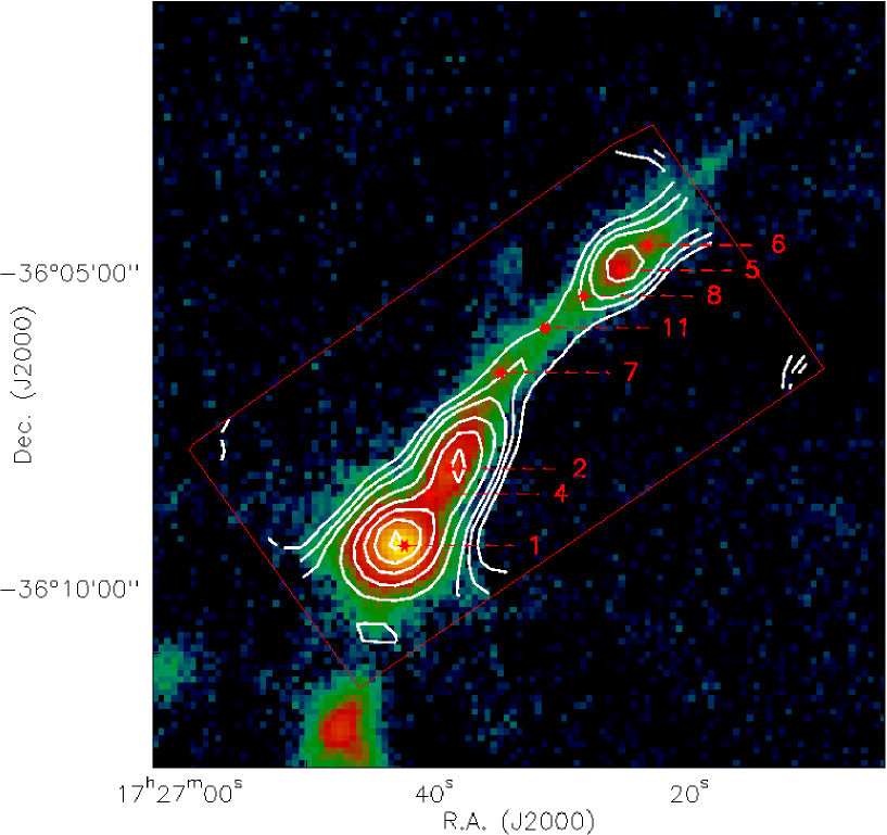
Figure 6: MOPRA N₂H⁺ moment zero map in contours overlaid on the LABOCA 870$\mu$m emission. The red rectangle shows the approximate area mapped with MOPRA. Clump labelling is the same as adopted through out the text. The contours have been chosen to start at 3 $\sigma$, 5 $\sigma$ in steps of 3 $\sigma$ where $\sigma=1.4\leavevmode\nobreak\ {\rm Jy\leavevmode\nobreak\ kms^{-1}}$.

The interaction of the molecular electric field gradient and the electric quadrupole moments of the nitrogen nuclei (I=1) leads to hyperfine structure and a splitting of the N₂H⁺ $(1-0)$ transition into seven components. The large line widths often attributed to the high level of turbulence in high-mass star-forming regions, lead to blending and result in three blended groups (one main and two satellites). As in the case of C¹⁷O, the CLASS HFS method has been used to fit the line profile. Thus, we can accurately determine the line optical depth, excitation temperature, line width, and LSR velocity. These parameters were determined for the four clumps averaged over the MOPRA beam of 35″. Subsequently, we determined the line column density following Caselli et al. (2002). The spectra of the three clumps are shown in Fig. 7, while the line parameters are tabulated in Table 8. The heavy blending of hyperfine components means less stringent constraints on the optical depth and excitation temperature. In particular, the optical depth for clump 1 derived from the HFS method in CLASS is unexpectedly low (0.2) with $>50$% error.  The fit to the hyperfine structure is as good for a range in optical depth, $0.2<\tau_{\rm tot}<1$. Hence, in Table 8 we give the range in column densities, abundance and abundance ratio bracketing $\tau_{\rm tot}=0.2$ and $\tau_{\rm tot}=1$. Fits for $\tau_{\rm tot}>1$ were poorer and discarded.

Figure 7: Spectra of N₂H⁺ 1–0 of clumps 1, 2, and 5 (clumps identified by CLUMPFIND). The black lines in each spectrum mark the seven hyperfine components.

Table 6: Column densities of C¹⁷O.

Clump	$N_{\rm{C^{17}O}}$
	($10^{15}$ cm-2)
	$T_{\rm{ex}}=10$ K	$T_{\rm{ex}}=25$ K	$T_{\rm{ex}}=35$ K
1	$38.8\pm 0.6$	$35.6\pm 0.6$	$41.3\pm 0.6$
2	$10.2\pm 0.1$	$9.3\pm 0.1$	$10.8\pm 0.1$
3	$5.1\pm 0.2$	$4.7\pm 0.2$	$5.4\pm 0.3$
5	$2.8\pm 0.2$	$2.6\pm 0.2$	$3.0\pm 0.3$
7	$4.25\pm 0.08$	$3.91\pm 0.08$	$4.5\pm 0.1$
9	$7.7\pm 0.1$	$7.03\pm 0.09$	$8.1\pm 0.1$
10	$1.7\pm 0.1$	$1.54\pm 0.09$	$1.8\pm 0.1$

Table 7: Column densities of C¹⁸O.

Clump	$N_{\rm{C^{18}O}}$
	($10^{15}$ cm-2)
	$T_{\rm{ex}}=10$ K	$T_{\rm{ex}}=25$ K	$T_{\rm{ex}}=35$ K
1	$104.0\pm 0.6$	$97.5\pm 0.6$	$113.4\pm 0.7$
2	$26.4\pm 0.4$	$24.7\pm 0.3$	$29.6\pm 0.4$
3	$12.5\pm 0.2$	$11.7\pm 0.2$	$13.6\pm 0.3$
4	$25.6\pm 0.3$	$24.1\pm 0.3$	$28.1\pm 0.4$
5	$14.5\pm 0.5$	$13.6\pm 0.5$	$15.8\pm 0.5$
6	$8.5\pm 0.5$	$8.0\pm 0.5$	$9.3\pm 0.5$
7	$15.0\pm 0.5$	$14.0\pm 0.5$	$16.3\pm 0.5$
8	$8.4\pm 0.4$	$7.9\pm 0.3$	$9.2\pm 0.4$
9	$18.4\pm 0.4$	$17.3\pm 0.3$	$20.1\pm 0.5$
10	$5.6\pm 0.4$	$5.2\pm 0.3$	$6.1\pm 0.5$
12	$13.7\pm 0.4$	$12.9\pm 0.3$	$15.0\pm 0.5$
G351.62	$5.2\pm 0.2$	$4.9\pm 0.2$	$5.7\pm 0.3$
	$1.0\pm 0.1$	$0.9\pm 0.1$	$1.1\pm 0.1$

6.1 CO–${\rm N_{2}H^{+}}$ enhancement

For reasons not yet fully understood, ${\rm N_{2}H^{+}}$ (along with ammonia), unlike CO, is resistant to depletion in very dense and cold cores (Öberg et al., 2005). However, internal heating re-introduces CO to the gas phase. Since CO is one of the main destroyers of ${\rm N_{2}H^{+}}$ in the gas phase (e.g., Aikawa et al., 2001), the abundance of N₂H⁺ decreases when protostellar/cluster formation heats up the envelope to sufficiently high temperatures, releasing the frozen out CO. The ratio of the observed CO-to-${\rm N_{2}H^{+}}$ abundance should thus reflect this chemistry. Hence, this differential depletion of the two species might therefore be used as a chemical clock to assess the evolutionary status of the clumps along the filament.

After smoothing the LABOCA data to the same resolution as the ${\rm N_{2}H^{+}}$ and C¹⁷O data, we estimated the molecular abundances of the two species and the relative abundance of C¹⁷O to N₂H⁺. Results are tabulated in Table 8. For this, we used the C¹⁷O column density assuming an excitation temperature of 20 K. Based on the absence/presence of MIR emission, hence on stellar content, we expected a significant spread in relative abundance between the clumps. Indeed, the ${\rm N_{2}H^{+}}$ column density correlates well with the MIR brightness with the column density increasing from clumps 5 to 1.

The ratio of ${\rm C^{17}O}$ and ${\rm N_{2}H^{+}}$ abundance is visualised in Fig. 6. To do this, we have taken the CO and N₂H⁺ abundance uncertainties into account. The statistical uncertainties based on fits to the line profile is sufficient for N₂H⁺. However for CO, while the errors on the fit to line profile is only a few percent, the unknown CO excitation temperature, $T_{ex_{\rm{CO}}}$, makes it the most significant parameter for estimating the uncertainties. We therefore vary the excitation temperature between 15 and 25 K and refer to Table 6 for extremes in ${\rm C^{17}O}$ column densities. For the densities observed in the cloud ($>10^{5}$  cm³), $T_{ex_{\rm{CO}}}$ must be very close to the gas temperature. Based on ammonia (1,1) and (2,2) observations with the Parkes telescope towards clumps 1, 2, and 3, Wienen et al. (in prep.) find a temperature of $<$20 K. For clumps 2 and 5, we thus adopt a reasonable temperature range of 10 K to 25 K to calculate the column densities. The mean of the largest difference in ${\rm C^{17}O}$ column densities at these very different temperatures (Table 6) is then considered as a conservative upper limit for the error on the ratio. A higher temperature extreme of 35 K is adopted for clump 1 which hosts the hot core associated with IRAS 17233–3606.

Uncertainties in the beam filling factor of N₂H⁺ and C¹⁷O is an additional source of error. For the C¹⁷O abundance, we expect a value close to 1 for the C¹⁷O column density (because of the low critical density of the line), and also for the H₂ column density given the size estimates obtained in Sect. 4.1; however, since we are limited by our single pointing measurements for CO and poor resolution for N₂H⁺, the respective beam filling factor remains unknown. For the N₂H⁺ abundance, dust emission and N₂H⁺ have very similar distributions. Also, the significant differences in source sizes extracted from our higher resolution dust observations (see Table 3) indicate that beam dilution might play a role. The abundance ratio decreases from 437/214 (clump 1) to 93 for clump 5 from the brightest end of the filament to the other end; however, based on the uncertainties discussed above, the observed differences in abundance ratio cannot be ascertained. The filament has an average ${\rm N_{2}H^{+}}$ abundance (over the three clumps) of 2.0$\times 10^{-10}$ relative to H₂. The derived column density and abundance is consistent with those found in other infrared dark clouds (Ragan et al. 2006; Sakai et al. 2008).

Table 8: ${\rm{N_{2}H^{+}}}$ 1–0 line parameters.

Clump	$\rm{v}_{\rm LSR}$	$\Delta\rm{v}$	$\tau_{\rm tot}$	$T_{\rm EX}$	$N_{\rm{N_{2}H^{+}}}$	$\chi_{\rm{N_{2}H^{+}}}$	$\chi_{\rm{C^{17}O}}$	$\chi_{\rm{C^{17}O}}$/$\chi_{\rm{N_{2}H^{+}}}$
	[km s-1]	[km s-1]		[K]	[1013 cm-2]	[10-10]	[10-8]
1	-3.7 (0.04)	4.55 (0.06)	0.2 - 1	11.7 - 37.3	5.5 - 11.3	0.83 - 1.68	3.6	214 - 437
2	-2.9 (0.01)	3.06 (0.05)	1.05 (0.02)	9.2 (0.4)	2.5 (0.2)	2.3	7.1	307
5	-2.2 (0.04)	3.36 (0.09)	1.41 (0.40)	6.1 (1.1)	1.8 (0.8)	3.7	3.4	93

Note $\tau_{\rm tot}$ is the sum of the peak optical depth of the seven hyperfine components, $\chi_{\rm{N_{2}H^{+}}}$ ($\chi_{\rm{C^{17}O}}$) is the N₂H⁺ (${\rm{C^{17}O}}$) abundance.

The fairly constant CO abundance over clumps with very distinct levels of star formation suggests that processes other than desorption of CO might affect the ${\rm N_{2}H^{+}}$ chemistry. In a CS and ${\rm N_{2}H^{+}}$ study of a small sample of dense cores in high-mass star-forming regions, Pirogov et al. (2007) briefly explore alternate pathways for the dissociative recombination of ${\rm N_{2}H^{+}}$ other than the standard channel with $\rm N_{2}$ as the end product (Geppert et al. 2004). However, these pathways may not be dominant, as previously thought (Adams et al. 2009), and new chemical models are required to explain this. Observationally, HCO⁺/H¹³CO⁺ distribution and abundance might help us in fully ruling out the role of CO desorption.

6.2 N₂H⁺ line width and velocity field

We have analysed the line width and velocity fields from the N₂H⁺ 3-D data, and the results are shown in Fig. 8. For these, we have considered only pixels corresponding to N₂H⁺ integrated intensity $>3\sigma$.

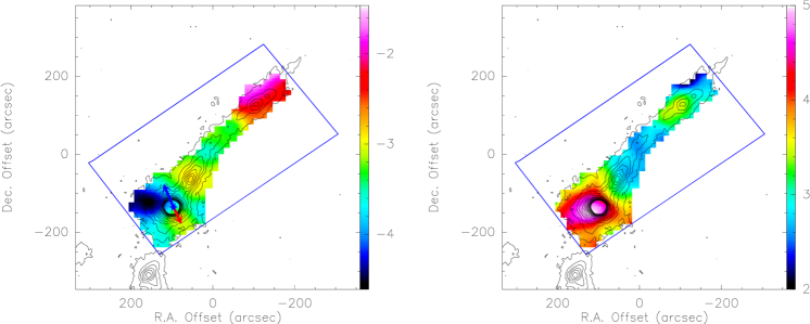
Figure 8: Left Panel: MOPRA N₂H⁺ velocity distribution with dust continuum LABOCA 870$\mu$m emission in contours. Red and blue arrows indicate the rough direction of the red and blue CO outflow lobes detected towards IRAS 17233–3606 respectively. Right Panel: MOPRA N₂H⁺ line width distribution (FWHM) with dust continuum LABOCA 870$\mu$m emission in contours. In both maps, background image units are in ${\rm kms^{-1}}$, and only those pixels that correspond to N₂H⁺ integrated intensity ${\rm>2.4Jy\leavevmode\nobreak\ kms^{-1}}$ have been considered significant.

Four clumps are identified in the first moment map (see Fig. 8, left panel). These have small differences in velocities compared to their line widths (Fig. 8, right panel). The velocity distribution for clump 1 is likely complicated by the intense star formation activity. If the filament were to be part of a shell-like structure (or if it were rotating), one would expect a clear linear velocity gradient from one end of the filament to the other. Most of the extended gas appears to be at a velocity of $-3.4\leavevmode\nobreak\$kms^-1, which we take to be the velocity of the ambient medium. Clumps 2 and 5 are separated by this lower density extended medium, contrary to a linear velocity gradient (see Sect. 7). A projection effect where clumps 2 and 5 are coincidentally aligned along a ring also seems unlikely given that there is no obvious kink in the velocity field.

Of particular interest are two striking features in the velocity map; (i) a large-scale ($\approx 1$ parsec) NE–SW velocity gradient of more than 1.6 ${\rm kms^{-1}}$ associated with the hot core in IRAS 17233–3606 (clump 1), and (ii) a smaller scale velocity gradient ($\approx 0.6$ parsec) in the northern clump (clumps 5, 6). Both velocity gradients are perpendicular to the filament, but in different directions. Interestingly, the NE(blue)-SW(red) gradient towards the hot core correlates well with the direction and kinematics of the CO outflows (Leurini et al., 2008, 2009). Although N₂H⁺ is seldom associated with outflows, the interactions of outflow shocks with the molecular envelope (traced by N₂H⁺) could explain such a gradient towards the hot core (clump 1) as detected in the same transition towards the class 0 object IRAM 04191+1522 by Lee et al. (2005). The axis of the outflow (shown in Fig. 8) would favour this shock scenario. This would also explain the very broad lines ($\approx 5$ ${\rm kms^{-1}}$) observed towards the hot core. Such broadening away from the mm core has also been observed in lower excitation NH₃ lines in low- and high-mass star-forming regions (Bachiller et al., 1993; Zhang et al., 1999; Beuther et al., 2007). A large-scale infall motion would also account for the observed velocity gradient. This large-scale infall is often observed in regions of high-mass star formation (Purcell et al., 2006).

The velocities at the peak positions between the northern and southern clumps differ by at least $>1.6$ ${\rm kms^{-1}}$. This is comparable to the average velocity dispersion (see Fig. 8 right panel, and Table 8) of the clumps within the filament. At this rate, the clumps would separate out on a scale of 1.6 pc in 1 Myrs.

The line width distribution shown in Fig. 8 might reflect differences in the evolutionary status of the clumps along the filament. As expected, the hot core (clump 1) exhibits the broadest line, and the rest of the filament (clumps 2, 5, and the rest of the cloud) has roughly similar line widths with a slightly higher peak towards clump 5. Clump 5 is associated with a stronger 8$\mu$m emission than clump 2; however, in all cases the line width is highly supersonic.

Given the line width and the extent of the cloud in projection, we can derive the crossing time. Thus the observed turbulents motions within the arc of filament would provide an upper limit to its lifetime of less than 1 Myr.

Unlike CO and its isotopologues studied here, the N₂H⁺ transition has a high critical density ($>10^{5}$  cm³). Therefore, in spite of the lower resolution of the N₂H⁺ data, we are selectively probing the dense gas, and not the envelope; i.e., line width-size relation does not necessarily apply. This might have the important implication that, although local star formation might be the cause of the exceptional line broadening in clumps 1 and 5, an external agent might be the cause of the line broadening along the whole filament. Interestingly, evidence of large-scale shocks, maybe remnants of the IRDC formation process, were found by Jiménez-Serra et al. (2010) towards IRDC G035.39–00.33. The present data set is insufficient to properly address this scenario. Future higher angular resolution observations capable of resolving the dense cores structures will allow us to test this scenario.

7 Discussion

Recently, Rathborne et al. (2010) have studied a sample of 38 IRDCs in continuum emission at submillimetre and mid– to far–IR wavelengths. They found that only a fifth of their clumps have 8$\mu$m emission, while almost half of them have a 24$\mu$m point source. In the case of G351.77, the majority of identified dust clumps are associated with emission at 24$\mu$m, suggesting that star formation is going on along the full extent of the filament. This is also confirmed by H₂ observations at 2.12$\mu$m which detected weak outflows along the full extent of the filament (Stanke et al. in prep.). The higher detection rate of 24$\mu$m compact sources in G351.77 compared to the sample studied by Rathborne et al. (2010) could be due to higher sensitivity to low-luminosity objects, given the closer distance of G351.77 ($D\leq 1$ kpc) compared to the typical distance ($\sim$4 kpc) of the IRDCs of Rathborne et al. (2010).

The velocity structure detected in N₂H⁺ shows very strong gradients towards individual clumps. This might indicate a general infall within the individual clumps (which might harbour a protocluster) or shocks in molecular envelopes. The line widths are highly supersonic and might also indicate the presence of such shocks.

The 8$\mu$m map (Fig. 3) shows emission along a semi-shell like structure, which is reminiscent of bubbles of gas and dust detected around expanding Hii regions (e.g., Elmegreen, 1998; Deharveng et al., 2003, 2005, 2010). These structures are potential candidates of star formation triggered by massive stars. The continuum emission at 870$\mu$m is also shaped along a semicircular structure. Therefore a tempting explanation for the broad line profiles associated with dust clumps in G351.77 is shock compression due to expansion of Hii regions on pre-existing gas. This could also be the triggering event for the intense star formation activity shown by several molecular outflows along the whole G351.77 (Stanke et al. in prep). We searched the SIMBAD database for all astronomical objects contained in a circle of 0.5^∘ diameter with clump 7 (in the middle of the dark filament) at its centre, but could not identify any obvious source of trigger. In particular, the only cm continuum sources in the region found in the NVSS catalogue (Condon et al., 1998) are associated with IRAS 17233–3606 and IRAS 17221–3619. From the velocity field derived from the CO observations, we know that the LABOCA semicircular structure is associated with molecular gas at two different velocities, one at $\sim-3$ km s^-1 (IRAS 17233–3606, G351.77 and clump 3), the other at $\sim-22$ km s^-1 (IRAS 17221–3619, IRAS 17227–3619 and the position G351.62). The near kinematic distance of IRAS 17221–3619 and IRAS 17227–3619 is $\sim 3.6$ kpc ($D_{\rm FAR}\sim 13$ kpc), while the two velocity components of the position G351.62 correspond to kinematic distances of $\sim 600$ pc and $\sim 3.6$ kpc ($D_{\rm FAR}\sim 16$ and 13 kpc, respectively), derived by using the rotation curve of Brand & Blitz (1993). For IRAS 17227–3619, Peeters et al. (2002) derived a kinematic distance of 3.4 kpc based on IR recombination lines, while Borissova et al. (2006) estimated distances between 1.9 and 3.2 kpc based on H- and K-band spectra of the source. Thus, the semicircular structure detected at 870$\mu$m in the LABOCA map is likely a projection effect of two different molecular clouds. However, from our pointed CO observations we can neither infer the true distribution of the two cloud complexes nor verify whether the western half circle, delineated by diffuse 8$\mu$m emission (see Sect. 3), is connected to one of these two clouds.

8 Conclusions

In summary, we have characterised the G351.77 dense filament in thermal dust continuum, N₂H⁺ $(1-0)$ and CO (various isotopologues at low excitation) emission. The molecular line emission traces the thermal dust continuum very well. Three main clumps in N₂H⁺ and eight clumps (at higher resolution) in the dust continuum were observed. These clumps also have associated emission from CO isotopologues. We analysed the integrated intensity, velocity, and line width distribution along the filament. The column density and mass of the clumps were also derived. The velocity structure shows very strong gradients across two clumps (1 and 5). This might indicate either a global infall within the individual clumps (which might harbour a protocluster) or shocks in molecular envelopes due to outflow-envelope interaction. All the clumps have supersonic line widths. Such supersonic line widths along the filament might also indicate the presence of shocks. Clearly, the most evolved clump is the hot core that shows (i) the brightest MIR emission, (ii) broadest line width, (iii) largest velocity gradient, and the (iv) most massive and dense core. Most mm clumps have a mass $>10$ $M_{\odot}$.

Our study shows that G351.77 has ongoing star formation in different evolutionary stages along the filament. Therefore, given the relatively close distance of this object compared to typical sites of massive star formation, G351.77 is an ideal target for investigating the role of IRDCs in the early phases of the formation of massive stars and stellar clusters, and for studying the population of low-mass stars in these objects.