Mitsui model with diagonal strains: A unified description of external pressure effect and thermal expansion of Rochelle salt NaKC₄H₄O${}_{6}\cdot 4$H₂O

Abstract

We elaborate a modification of the deformable two-sublattice Mitsui model of [Levitskii R.R. et al., Phys. Rev. B. 2003, 67, 174112] and [Levitskii R.R. et al., Condens. Matter Phys., 2005, 8, 881] that consistently takes into account diagonal components of the strain tensor, arising either due to external pressures or due to thermal expansion. We calculate the related to those strains thermal, piezoelectric, and elastic characteristics of the system. Using the developed fitting procedure, a set of the model parameters is found for the case of Rochelle salt crystals, providing a satisfactory agreement with the available experimental data for the hydrostatic and uniaxial pressure dependences of the Curie temperatures, temperature dependences of spontaneous diagonal strains, linear thermal expansion coefficients, elastic constants $c_{ij}^{E}$ and $c_{i4}^{E}$, piezoelectric coefficients $d_{1i}$ and $g_{1i}$ ($i=1,2,3$). The hydrostatic pressure variation of dielectric permittivity is described using a derived expression for the permittivity of a partially clamped crystal. The dipole moments and the asymmetry parameter of Rochelle salt are found to increase with hydrostatic pressure.

Rochelle salt, thermal expansion, hydrostatic pressure, uniaxial pressure, Mitsui model 65.40.De, 77.80.B-, 77.65.Bn, 65.40.Ba, 77.22.Ch

Abstract

Запропоновано модифiкацiю деформiвної двопiдґраткової моделi Мiцуї робiт [Levitskii R.R. et al, Phys. Rev. B. 2003, 67, 174112] та [Levitskii R.R. et al., Condens. Matter Phys., 2005, 8, 881], яка послiдовно враховує дiагональнi компоненти тензора деформацiй, що виникають пiд дiєю зовнiшнiх тискiв чи внаслiдок теплового розширення. Розраховано пов’язанi з цими деформацiями тепловi, п’єзоелектричнi та пружнi характеристики системи. Використовуючи запропоновану схему, для кристалiв сеґнетової солi знайдено такий набiр параметрiв теорiї, що забезпечує задовiльне узгодження з експериментальними даними для залежностей температур Кюрi вiд гiдростатичного та одновiсних тискiв, а також температурних залежностей теплових деформацiй, лiнiйних коефiцiєнтiв теплового розширення, пружних сталих $c_{ij}^{E}$ i $c_{i4}^{E}$, п’єзоелектричних коефiцiєнтiв $d_{1i}$ i $g_{1i}$ ($i=1,2,3$). Залежностi дiелектричної проникностi вiд гiдростатичного тиску описано за допомогою отриманого в роботi виразу для проникностi частково затиснутого кристалу. Виявлено, що дипольнi моменти та параметр асиметрiї в сеґнетовiй солi зростають з гiдростатичним тиском.

сеґнетова сiль, теплове розширення, гiдростатичний тиск, одновiсний тиск, модель Мiцуї

1 Introduction

The Mitsui model [1] (two-sublattice Ising model with asymmetric potentials) has been originally proposed for description of the reentrant phase behavior in Rochelle salt crystals. It considers the motion of certain ordering units in two interpenetrating sublattices of asymmetric double-well potentials. The model with certain modifications is also applicable to several other ferroelectrics [2], like those of the Rochelle salt type (deuterated and ammonium-doped [3] Rochelle salt at least at low doping ), RbHSO₄ type [4, 5], AgNa(NO${}_{2})_{2}$ (SSN [6, 7]), SASD type [8] (NaNH₄SO₄$\cdot$2H₂O and NaNH₄SeO₄$\cdot$2H₂O), etc.

Very often, inclusion of deformational effects into the Mitsui model is indispensable for a proper description of the system behavior even at ambient pressure. Thus, a strong piezoelectricity associated with polarization $P_{1}$ and shear strain $\varepsilon_{4}$ essentially affects the dynamic dielectric response of Rochelle salt due to the effect of crystal clamping by the high-frequency measuring field. The conventional Mitsui model yields a qualitatively incorrect behavior of the relaxation time and dynamic dielectric permittivity near the Curie temperatures. This problem is resolved [9] by taking into account the piezoelectric coupling with $\varepsilon_{4}$, also permitting to describe the phenomena of piezoelectric resonance and sound attenuation [10].

The sequence of phase transitions observed in NH₄HSO₄ crystals can be described within the mean field approximation for the Mitsui model only with temperature dependent interaction constants [5]. It means that one must take into account the effect of thermal expansion, which is, ultimately, a deformational effect.

Since high pressure studies are the only means to continuously vary the system geometrical parameters, such as the orientation angles of atomic groups that form the dipole moments, interatomic distances, hydrogen bonds parameters, etc, as well as the interparticle interactions, and other parameters of the system, they can provide a valuable information on the mechanism of the phase transitions in ferroelectric crystals. A better insight is obtained if the effects of hydrostatic and various uniaxial and biaxial pressures are explored. Irrespectively of the crystal symmetry, these pressures produce diagonal components of the lattice strain tensor $\varepsilon_{i}$ ($i=1,2,3$). In low-symmetry systems, shear strains $\varepsilon_{j}$ ($j=4,5,6$) can be induced as well. The diagonal strains also arise due to the thermal expansion of the crystals.

Nowadays, Rochelle salt [11, 12, 13, 14] and other crystals [15] described by the Mitsui model often serve as test materials for experiments with nanosize phenomena. Properties of the ferroelectric nano-inclusions in a solid matrix are strongly affected by surface tension and thermal mismatch stresses. Thus, radial stresses in the plane perpendicular to spontaneous polarization arise in Rochelle salt nanorods grown in pores of alumina films [11, 12], inducing diagonal strains only. A phenomenological theory of ferroelectric properties of such nanorods was presented in [16].

The simplest way to incorporate an external pressure into a spin model is to consider its parameters (interaction constants) phenomenologically as linear functions of pressure. This approach has been used for different versions of the Mitsui model to describe the hydrostatic pressure variation of the transition temperatures in Rochelle salt [17] and SASD [18]. However, to describe a uniaxial stress dependence of $T_{\rm C}$ in the same way, one would have to find new values of the fitting parameters for each stress direction. A unified model description of hydrostatic and uniaxial pressure effects, and, at the same time, the crystal thermal expansion at ambient pressure, with a single set of the fitting parameters is possible if we include into the model the lattice diagonal strains, instead of the pressures. Such a microscopic-like model of bulk crystals that includes the diagonal strains will be very helpful when one develops a model description of the above mentioned nanocrystal behavior.

The goal of the present paper is to develop a modification of the deformable Mitsui model with the shear strain $\varepsilon_{4}$ [9], which would also take into account the diagonal components of the lattice strain tensor. The first attempt to create such a modification was made in [19]. The interaction constants and the asymmetry parameter were taken to be linear functions of the diagonal strains. Expressions for the piezoelectric and elastic characteristics of Rochelle salt, associated with these strains, have been obtained. However, all actual calculations were performed in the approximation of zero thermal strains; the external hydrostatic or uniaxial pressure effect was not considered, and the fitting procedure was inappropriate. Here we shall use the model of [19] and take into account the thermal expansion strains properly. We shall develop a consistent fitting procedure, free from the drawbacks of the previous [19] calculations, allowing us to obtain the above mentioned unified description of high pressure effects, thermal expansion, as well as physical properties of Rochelle salt associated with the diagonal strains.

Bulk Rochelle salt undergoes two second-order phase transitions at $T_{\rm C1}=255$ K and $T_{\rm C2}=297$ K, with the intermediate ferroelectric phase. Spontaneous polarization $P_{1}$ is directed along the $a$ axis, accompanied by spontaneous shear strain $\varepsilon_{4}$ in the $bc$ plane. The crystal is orthorhombic (space group $P2_{1}2_{1}2_{1}$) in the paraelectric phases and monoclinic ($P2_{1}11$) in the ferroelectric phase. As it follows from the analysis of symmetry elements of its point group 222 and of the uniaxial pressure point group $\infty/mmm$, no uniaxial or biaxial pressure applied along the orthorhombic crystallographic axes of a Rochelle salt crystal changes its symmetry. Neither do the hydrostatic pressure or thermal expansion of the crystal.

The mechanism of phase transitions in Rochelle salt remains rather obscure. According to the most recent measurements [20, 21], the largest displacements at a ferroelectric phase transition are undergone by the O₈, O₉, O₁₀ oxygens. It appears that the dipoles of the Mitsui model, moving in the double-well potentials, should plausibly be associated with the OH₉ and OH₁₀ groups. Their motion, coupled with displacive vibrations of OH₈ groups seems to be responsible for the phase transitions, as well as for the spontaneous polarization. It would be interesting to elucidate the pressure variation of the dipole moments, as well as of the asymmetry parameters of the double-well potentials. This can shed some light on the details of the transition mechanism.

The set of experimental data for Rochelle salt, used for verification of the present modification of the Mitsui model, includes the hydrostatic pressure dependences of transition temperatures [22, 23] and dielectric permittivity [23], the uniaxial [24, 25] and biaxial [26] pressure dependences of the Curie temperatures. Related to the diagonal strains, components of piezoelectric (e.g. $d_{1i}$, $i=1,2,3$) and elastic ($c_{i4}$) tensors [27, 28, 29], appearing in the ferroelectric phase only, should be also described by the model. The other characteristics, included into the fitting, are thermal expansion coefficients and dilatations [30, 31], as well as the diagonal-strain-related elastic constants[32] $c_{ij}$ or compliances $s_{ij}$ ($i,j=1,2,3$).

We introduce the diagonal strains $\varepsilon_{1}$, $\varepsilon_{2}$, $\varepsilon_{3}$ into the two-sublattice Mitsui model with the shear strain $\varepsilon_{4}$ [9] in the manner it was done in [19]. In section 2 we make a further modification of the model by taking into account the host lattice contributions into the thermal expansion. Section 3 contains the obtained expressions for thermal, elastic, dielectric, and piezoelectric characteristics. In section 4 we propose a new fitting procedure. Using the found set of the fitting parameters for the Rochelle salt crystals, we show that the developed theory is capable of describing the entire complex of the phenomena, related to the diagonal strains: thermal expansion, temperature behavior of monoclinic piezoelectric and elastic characteristics, hydrostatic, uniaxial, and biaxial pressure dependences of the Curie temperatures in Rochelle salt. The behavior of the dielectric permittivity under hydrostatic pressure is described using the derived expression for the permittivity of a partially clamped crystal.

2 System thermodynamics in the presence of diagonal strains

We consider an orthorhombic piezoelectric crystal in the paraelectric phase, to which an external hydrostatic or uniaxial or biaxial (along the crystallographic axes) pressure can be applied. All these pressures produce diagonal strains $\varepsilon_{i}$ ($i=1,2,3$); these strains are also present due to the thermal expansion. Paraelectric piezoelectricity is associated with the shear strain $\varepsilon_{4}$. The Rochelle salt symmetry is presumed having the spontaneous polarization directed along the $a$ axis and coupled to the strain $\varepsilon_{4}$.

We start with the modified two-sublattice Mitsui model with a piezoelectric coupling to the shear strain $\varepsilon_{4}$ and with the diagonal strains [9, 19]. A unit cell of the model consists of two dipoles (two sublattices), oppositely oriented along the $a$-axis (the axis of spontaneous polarization); they are compensated in the paraelectric phases and get non-compensated in the ferroelectric phase. The actual unit cell of a real Rochelle salt crystal is twice as large and contains four dipoles. At the transition to the monoclinic phase the angle between the $b$ and $c$ axes changes from $\pi/2$ to $\pi/2-\varepsilon_{4}$. The diagonal strains $\varepsilon_{1}$, $\varepsilon_{2}$, $\varepsilon_{3}$ describe the relative changes in the lattice constants $a$, $b$, and $c$, respectively, due to thermal expansion or under pressure.

In the mean field approximation, the model Hamiltonian reads [9]

$$\hat{H}_{\mathrm{m}}=NU_{\mathrm{seed}}+\frac{N}{8}J(\eta_{1}^{2}+\eta_{2}^{2})+\frac{N}{4}K\eta_{1}\eta_{2}-\sum\limits_{q}\Bigl{[}E(1)\frac{\sigma_{q1}}{2}-E(2)\frac{\sigma_{q2}}{2}\Bigr{]},$$ (1)

where $\eta_{f}\equiv\langle\sigma_{qf}\rangle$; $N$ is the number of the unit cells; $J$, $K$ are the Fourier-transforms (at ${\bf k}=0$) of the constants of interaction between pseudospins belonging to the same and to different sublattices, respectively.

The phenomenological part of the Hamiltonian $U_{\mathrm{seed}}$ is a ‘‘seed’’ energy of the host lattice of heavy ions which forms the asymmetric double-well potentials for the pseudospins. For the case of Rochelle salt symmetry in presence of diagonal strains, shear strain $\varepsilon_{4}$, and field $E_{1}$, it reads

$${U_{\mathrm{seed}}}=\frac{v_{0}}{2}c_{44}^{E0}\varepsilon_{4}^{2}-{v_{0}}e_{14}^{0}\varepsilon_{4}E_{1}-\frac{v_{0}\varepsilon_{0}}{2}\chi_{11}^{\varepsilon 0}E_{1}^{2}+\frac{v_{0}}{2}\sum_{i,j=1}^{3}c_{ij}^{E0}\varepsilon_{i}\varepsilon_{j}-v_{0}\sum_{ij=1}^{3}c_{ij}^{E0}\alpha_{i}^{0}(T-T_{i}^{0})\varepsilon_{j}\,.$$ (2)

Here $\varepsilon_{0}$ is the vacuum permittivity; $v_{0}$ is the unit cell volume of the model. The three first terms in $U_{\mathrm{seed}}$ are the elastic, piezoelectric, and electric contributions due to the shear strain $\varepsilon_{4}$ and longitudinal electric field $E_{1}$. Two last terms are related to the diagonal strains. Here $c_{44}^{E0}$, $c_{ij}^{E0}$, $e_{14}^{0}$ are the ‘‘seed’’ constants describing the phenomenological contributions of the crystal lattice into the corresponding observed quantities $c_{44}^{E}$, $c_{ij}^{E}$, and $e_{14}$. In fact, the index $E$ in $c_{ij}^{E0}$ is redundant, as the difference between the observed $c_{ij}^{E}$ and $c_{ij}^{P}$ at $i,j=1,2,3$ is negligible. The ‘‘seed’’ quantities are zeros if the corresponding observed quantities are zeros in the most symmetric phase (orthorhombic in the case of Rochelle salt).

The last term, absent in the earlier model [19], is the contribution of the host lattice into the energy of thermal expansion. $\alpha_{i}^{0}$ are the ‘‘seed’’ thermal expansion coefficients; $T_{i}^{0}$ are the temperatures at which the components of this contribution vanish. It is known that the thermal strains can be set to be equal to zero at any arbitrary temperature $T_{0}$ (the reference point for thermal expansion). This can be achieved by choosing the values of $T_{i}^{0}$ accordingly; they will differ from $T_{0}$ due to the pseudospin system contributions to the thermal expansion. To take into account the ‘‘seed’’ contribution of the host lattice is indispensable for a proper description of thermal expansion.

The coefficients

$$E(1)=\frac{1}{2}J\eta_{1}+\frac{1}{2}K\eta_{2}+\Delta-2\psi_{4}\varepsilon_{4}+\mu_{1}E_{1},\qquad E(2)=\frac{1}{2}J\eta_{2}+\frac{1}{2}K\eta_{1}-\Delta-2\psi_{4}\varepsilon_{4}+\mu_{1}E_{1}$$ (3)

in (1) are the local mean fields acting on pseudospins of the first and second sublattices in the $q^{\mathrm{th}}$ unit cell. The parameter $\Delta$ describes the asymmetry of the double well potential; $\mu_{1}$ is the effective dipole moment. The model parameter $\psi_{4}$ describes the internal field created by the piezoelectric coupling with $\varepsilon_{4}$ and essentially determines the piezoelectric and elastic characteristics associated with the shear strain $\varepsilon_{4}$ [9, 19]. It is also assumed that a longitudinal electric field $E_{1}$ is applied.

$$J\pm K=J_{0}\pm K_{0}+2\sum\limits_{i=1}^{3}{\psi_{i}^{\pm}\varepsilon_{i}}\,,\quad$$ (4)

as well as the asymmetry parameter

$$\Delta=\Delta_{0}+\sum\limits_{i=1}^{3}{\psi_{3i}\varepsilon_{i}}$$ (5)

are taken to be linear functions of the diagonal strains [19]. Here $\psi_{3i}^{\pm}$ are introduced simply as the expansion coefficients. However, for $J$ and $K$ such an expansion is equivalent to taking into account the electrostrictive coupling with the diagonal strains. For $\Delta$ it implicitly describes the changes in the asymmetry parameter due to the changes produced by external pressure or thermal expansion in the interatomic distances and in the geometric parameters of the potential, like the distance between the potential wells, etc. The parameters $\psi_{3i}$, are analogous to the deformational potentials $2\gamma=\partial\Delta/\partial\varepsilon$ introduced in the Anderson-Halperin-Varma-Phillips [33, 34] model of two-level systems with asymmetric double-well potentials in order to describe ultrasound attenuation and thermal conductivity in amorphous solids at very low temperatures.

The thermodynamic potential of the considered model is obtained within the mean field approximation in the following form

$$g_{2E}(p_{i},T)=U_{\mathrm{seed}}+\frac{J+K}{4}\xi^{2}+\frac{J-K}{4}\sigma^{2}-\frac{2\ln 2}{\beta}-\frac{1}{\beta}\ln\cosh\frac{\gamma+\delta}{2}\cosh\frac{\gamma-\delta}{2}+v_{0}\sum_{i=1}^{4}p_{i}\varepsilon_{i}\,,$$ (6)

where $\beta=1/k_{\mathrm{B}}T$, $k_{\mathrm{B}}$ is the Boltzmann constant, and

$$\gamma=\beta\left(\frac{J+K}{2}\xi-2\psi_{4}\varepsilon_{4}+\mu_{1}E_{1}\right),\qquad\delta=\beta\left(\frac{J-K}{2}\sigma+\Delta\right).$$

Here $p_{1}=p_{2}=p_{3}=p_{\mathrm{h}}$ for hydrostatic pressure; $p_{1}\neq 0$ and $p_{2}=p_{3}=0$ for the uniaxial pressure applied along the axis $a$, etc. The shear pressure $p_{4}$ is introduced formally, in order to find the elastic and piezoelectric characteristics associated with it; after that it is put equal to zero.

We introduced the following linear combinations of the mean pseudospin values

$$\xi=\frac{1}{2}(\eta_{1}+\eta_{2}),\qquad\sigma=\frac{1}{2}(\eta_{1}-\eta_{2});$$

$\xi$ is the parameter of ferroelectric ordering in the system. The parameters $\xi$ and $\sigma$ are determined from the saddle point of the thermodynamic potential (6): a minimum of $g_{2E}$ with respect to $\xi$ and a maximum with respect to $\sigma$ are realized at equilibrium. The corresponding equations are

$$\xi=\frac{\sinh\gamma}{\cosh\gamma+\cosh\delta}\,,\qquad\sigma=\frac{\sinh\delta}{\cosh\gamma+\cosh\delta}\,.$$ (7)

3 Physical characteristics of Rochelle salt related to diagonal strains

Using the following thermodynamic relations

$$\frac{1}{v}\left({\frac{\partial g_{2E}}{\partial\varepsilon_{i}}}\right)_{E1}=0,\qquad-\frac{1}{v}\left({\frac{\partial g_{2E}}{\partial E_{1}}}\right)_{\sigma}=P_{1}\qquad(i=1\div 4),$$

where $v=v_{0}(1+\sum_{i=1}^{3}\varepsilon_{i})$ is the pressure and temperature dependent unit cell volume, and retaining only linear in $\varepsilon_{i}$ terms in the ‘‘seed’’ contributions, we obtain expressions for strains and polarization

$$\varepsilon_{i}=-\sum\limits_{j=1}^{3}s_{ij}^{E0}p_{j}+\alpha_{i}^{0}(T-T_{i}^{0})+\frac{1}{2v_{0}}\sum_{j=1}^{3}s_{ij}^{E0}(\psi_{j}^{+}\xi^{2}+\psi_{j}^{-}\sigma^{2}+2\psi_{3j}\sigma),\quad({i}=1\div 3),$$ (8)

$$\varepsilon_{4}=-\frac{p_{4}}{c_{44}^{E0}}+\frac{e_{14}^{0}}{c_{44}^{E0}}E_{1}-\frac{2\psi_{4}}{v_{0}c_{44}^{E0}}\xi\,,$$ (9)

$$P_{1}=e_{14}^{0}\varepsilon_{4}+\varepsilon_{0}\chi_{11}^{\varepsilon 0}E_{1}+\frac{\mu_{1}}{v}\xi\,.$$ (10)

Here $s_{ij}^{E0}$ are the elements of the matrix inverse to the matrix of ‘‘seed’’ elastic constants $c_{ij}^{E0}$.

Two first terms in equation (8) represent the host system contributions into the Hooke’s law and thermal expansion with regular pressure and temperature behavior. The sum in equation (8) gives the pseudospin subsystem contributions into the strains, having anomalous behavior in the ferroelectric phase. The second term in equation (8) was absent in the previous model [19].

From equations (8)–(10) we can derive expressions for other characteristics related to the diagonal strains. Thus, the coefficients of linear thermal expansion are obtained in a rather cumbersome form

$$\alpha_{i} = \left(\frac{\partial\varepsilon_{i}}{\partial T}\right)_{\mathrm{p}}=\sum_{k=1}^{3}B_{ik}\Bigg{\{}\alpha_{k}^{0}+\frac{1}{2v_{0}T(\varphi_{2}-\Lambda\varphi_{3})}$$ (11)

$${}\times\sum_{j=1}^{3}s_{kj}^{E0}\left[\psi_{j}^{+}\xi(\lambda_{2}\delta-\varphi_{3}\gamma)+(\psi_{j}^{-}\sigma+\psi_{3j})(\lambda_{2}\gamma-\tilde{\varphi}_{5}\delta)\right]\Bigg{\}},$$

where

$$\hat{B}=\left[\hat{I}+\hat{s}^{E0}\hat{\tilde{c}}\right]^{-1},$$

$$\tilde{c}_{jk}=-\frac{\beta}{2v_{0}(\varphi_{2}-\Lambda\varphi_{3})}\Bigl{\{}(\psi_{i}^{+}\varphi_{4j}+\psi_{j}^{+}\varphi_{4i})\xi-\psi_{i}^{+}\psi_{j}^{+}\xi^{2}\varphi_{3}+(\psi_{i}^{-}\sigma+\psi_{3i})(\psi_{j}^{-}\sigma+\psi_{3j})\tilde{\varphi}_{5}\Bigr{\}},$$

$$\tilde{\varphi}_{5}=\lambda_{1}-\left[\frac{\beta(K+J)}{4}+\Lambda\right](\lambda_{1}^{2}-\lambda_{2}^{2});$$

$\hat{I}$ is a unit matrix. The other notations are

$$\varphi_{4i}=\psi_{i}^{+}\xi\varphi_{3}-\left({\psi_{i}^{-}\sigma+\psi_{3i}}\right)\lambda_{2}\,,$$

$$\varphi_{2}=1-\frac{\beta J}{2}\lambda_{1}-\beta^{2}\frac{K^{2}-J^{2}}{16}(\lambda_{1}^{2}-\lambda_{2}^{2}),\qquad\varphi_{3}=\lambda_{1}+\frac{\beta(K-J)}{4}(\lambda_{1}^{2}-\lambda_{2}^{2}),$$

$$\lambda_{1}=1-\xi^{2}-\sigma^{2},\qquad\lambda_{2}=2\xi\sigma,\qquad\Lambda=\frac{2\beta\psi_{4}^{2}}{v_{0}c_{44}^{E0}}\,.$$

Alternatively, the coefficients of thermal expansion can be found by numerical differentiation of equation (8) for the strains $\varepsilon_{i}$ with respect to temperature; the results, of course, coincide. The coefficients $\alpha_{i}$ are expected to have small anomalies at the Curie temperatures [31, 30].

The molar specific heat at constant pressure of the model is obtained from the molar entropy

$$S\!=\!-\frac{N_{\mathrm{A}}}{2}\Bigl{(}\frac{\partial g_{1E}(\varepsilon_{i},T)}{\partial T}\Bigr{)}_{\varepsilon_{i}}\!\!=\frac{v_{0}N_{\mathrm{A}}}{2}\sum_{ij=1}^{3}c_{ij}^{E0}\alpha_{i}^{0}\varepsilon_{j}+\frac{R}{2}\left(2\ln 2+\ln\cosh\frac{\gamma+\delta}{2}\cosh\frac{\gamma-\delta}{2}-\gamma\xi-\delta\sigma\right)\!,$$

where $g_{1E}(\varepsilon_{i},T)=g_{2E}(\sigma_{i},T)-v_{0}\sum_{i}p_{i}\varepsilon_{i}$; $R$ is the universal gas constant, and $N_{\mathrm{A}}$ is the Avogadro constant. Thus, the molar specific heat of the model is

$$c_{\mathrm{p}} = T\left(\frac{\partial S}{\partial T}\right)_{\mathrm{p}}=\frac{v_{0}N_{\mathrm{A}}T}{2}\sum_{ij=1}^{3}c_{ij}^{E0}\alpha_{i}^{0}\alpha_{j}+\frac{R}{4(\varphi_{2}-\Lambda\varphi_{3})}\left\{(\lambda_{2}\delta-\varphi_{3}\gamma)\left(\gamma+\xi\sum_{i=1}^{3}\frac{\alpha_{i}}{k_{\mathrm{B}}}\psi_{i}^{+}\right)\right.$$ (12)

$${}\left.-(\lambda_{2}\gamma-\tilde{\varphi}_{5}\delta)\left[\delta-\sum_{i=1}^{3}\frac{\alpha_{i}}{k_{\mathrm{B}}}(\psi_{i}^{-}\sigma+\psi_{3i})\right]\right\}.$$

As we shall see, it has small anomalies at the transition points. To obtain the total specific heat of a crystal that can be compared to experimental data, we have to add to equation (12) a regular term linear in temperature (within the considered temperature range) that would correspond to a contribution of lattice vibrations not taken into account within our model. Thus,

$$c_{\mathrm{p}}^{\mathrm{tot}}=c_{\mathrm{p}}+c_{\mathrm{vibr}}\,,\qquad c_{\mathrm{vibr}}=A+BT;$$ (13)

the coefficients $A$ and $B$ will be specified by fitting equation (13) to experimental data. Often, an inverse procedure is performed, when a regular linear contribution is subtracted from the experimental data; the obtained result is then compared with the theoretical specific heat of the ordering subsystem.

The other found characteristics are, in particular, the elastic constants at constant electric field ($i,j=1,2,3$)

$$c_{ij}^{E} = -\Bigl{(}\frac{\partial p_{i}}{\partial\varepsilon_{j}}\Bigr{)}_{E,T}$$ (14)

$$= c_{ij}^{E0}-\frac{\beta}{2v_{0}\varphi_{2}}\Bigl{[}(\psi_{i}^{+}\varphi_{4j}+\psi_{j}^{+}\varphi_{4i})\xi-\psi_{i}^{+}\psi_{j}^{+}\xi^{2}\varphi_{3}+(\psi_{i}^{-}\sigma+\psi_{3i})(\psi_{j}^{-}\sigma+\psi_{3j})\varphi_{5}\Bigr{]},$$

$$c_{i4}^{E} = \frac{\beta\psi_{4}}{v_{0}}\frac{\varphi_{4i}}{\varphi_{2}},$$ (15)

as well as the monoclinic piezoelectric coefficients

$$e_{1i}=\left(\frac{\partial P_{1}}{\partial\varepsilon_{i}}\right)_{E_{1},T}=\frac{\mu_{1}}{v}\left(\frac{\beta\varphi_{4i}}{2\varphi_{2}}-\frac{\xi}{1+\sum_{i=1}^{3}\varepsilon_{i}}\right),$$

$$d_{1i}=\left(\frac{\partial\varepsilon_{i}}{\partial E_{1}}\right)_{p_{i},T}=\sum\limits_{j=1}^{4}{s_{ij}^{E}e_{1j}}\,,$$ (16)

where $s_{ij}^{E}$ is the matrix of elastic compliances, inverse to the matrix of elastic constants $c_{ij}^{E}$, and

$$\varphi_{5}=\lambda_{1}-\frac{\beta(K+J)}{4}\left(\lambda_{1}^{2}-\lambda_{2}^{2}\right).$$

The other piezoelectric and elastic characteristics are

$$h_{1i}=-\left(\frac{\partial E_{1}}{\partial\varepsilon_{i}}\right)_{P_{1}}=\frac{e_{1i}}{\varepsilon_{0}\chi_{11}^{\varepsilon}}\,,\qquad g_{1i}=-\left(\frac{\partial E_{1}}{\partial p_{i}}\right)_{P_{1}}=\frac{d_{1i}}{\varepsilon_{0}\chi_{11}^{\sigma}}\,,\qquad c_{ij}^{P}=\left(\frac{\partial p_{i}}{\partial\varepsilon_{j}}\right)_{P,T}=c_{ij}^{E}+e_{1i}h_{1j}\,.$$

Here,

$$\chi_{11}^{\varepsilon}=\frac{1}{\varepsilon_{0}}\left(\frac{\partial P_{1}}{\partial E_{1}}\right)_{\varepsilon}=\chi_{11}^{\varepsilon 0}+\frac{\beta\mu_{1}^{2}}{2v\varepsilon_{0}}\frac{\varphi_{3}}{\varphi_{2}}$$ (17)

is the dielectric susceptibility of a clamped crystal, and

$$\chi_{11}^{\sigma}=\frac{1}{\varepsilon_{0}}\left(\frac{\partial P_{1}}{\partial E_{1}}\right)_{\mathrm{p}}=\chi_{11}^{\sigma 0}+\frac{\beta(\mu_{1}^{\prime})^{2}}{2v\varepsilon_{0}}\frac{\displaystyle\varphi_{3}}{\displaystyle\varphi_{2}-\Lambda\varphi_{3}}+\frac{1}{\varepsilon_{0}}\sum\limits_{i=1}^{3}{e_{1i}d_{1i}}$$ (18)

is the static dielectric susceptibility of a mechanically free crystal [19]. Here we introduce the following notations

$$\quad{\mu_{1}^{\prime}}={\mu_{1}}-{2}\psi_{4}d_{14}^{0}\,,\qquad d_{14}^{0}=\frac{e_{14}^{0}}{c_{44}^{E0}}\,,\qquad\chi_{11}^{\sigma 0}=\chi_{11}^{\varepsilon 0}+\frac{1}{\varepsilon_{0}}e_{14}^{0}d_{14}^{0}\,.$$

In paraelectric phases, this expression for the free susceptibility coincides with that obtained within the modified Mitsui model without thermal strains [10]. The sum ${\varepsilon_{0}^{-1}}\sum e_{1i}d_{1i}\,$, different from zero in the ferroelectric phase and not exceeding 5% of the total susceptibility, was absent in the earlier model.

As one can easily verify, monoclinic quantities $e_{1i}$, $d_{1i}$, $h_{1i}$, $g_{1i}$, $c_{i4}^{E}$, $c_{i4}^{P}$ ($i=1,2,3)$ differ from zero only at non-zero polarization, in agreement with the symmetry considerations.

The temperature of the second order phase transition is determined from the condition that dielectric susceptibility of a free crystal $\chi_{11}^{\sigma}$ diverges at $T\to T_{\rm C}$. From equation (18) and using equation (7) we obtain

$$\cosh^{2}\left(\frac{J-K}{4k_{\mathrm{B}}T_{\rm C}}\sigma_{\mathrm{c}}+\frac{\Delta}{2k_{\mathrm{B}}T_{\rm C}}\right)=\frac{K+J}{4k_{\mathrm{B}}T_{\rm C}}+\frac{2\psi_{4}^{2}}{v_{0}c_{44}^{E0}k_{\mathrm{B}}T_{\rm C}}\,,$$ (19)

where the model parameters $J$, $K$, $\Delta$ are taken at $T_{\rm C}$, being renormalized by diagonal strains according to equation (4).

Equation (19) is valid both for the ambient pressure case and for the stressed crystal. It can be rewritten in the two following convenient forms:

$$\sigma_{\mathrm{c}}=\sqrt{1-\frac{k_{\mathrm{B}}T_{\rm C}}{\frac{K+J}{4}+\frac{2\psi_{4}^{2}}{v_{0}c_{44}^{E0}}}}\,,$$ (20)

which gives an explicit expression for $\sigma$ at the transition points, and

$$\sum_{i}\delta_{3i}\varepsilon_{ci}+\sigma_{\mathrm{c}}\sum_{i}\psi_{i}^{-}\varepsilon_{ci}=-\Delta_{0}-\frac{J_{0}-K_{0}}{2}\sigma_{\mathrm{c}}+2k_{\mathrm{B}}T_{\rm C}{\rm Arccosh}{\sqrt{\frac{K+J}{4k_{\mathrm{B}}T_{\rm C}}+\frac{2\psi_{4}^{2}}{v_{0}c_{44}^{E0}k_{\mathrm{B}}T_{\rm C}}}}\,,$$

useful in the fitting procedure. Here $\varepsilon_{ci}$ are the strains at the Curie temperature.

4 Numerical calculations

4.1 Fitting procedure

The model parameters must provide a fit of the theory to the experimental data for the following characteristics: the Curie temperatures at ambient pressure $T_{{\rm C}k}$ ($k=1,2$ in Rochelle salt) and their hydrostatic and uniaxial pressure slopes $\partial T_{{\rm C}k}/\partial p_{\mathrm{h}}$ and $\partial T_{{\rm C}k}/\partial p_{j}$, the temperature curves of thermal expansion strains $\varepsilon_{i}$, linear thermal expansion coefficients, monoclinic piezomodules $g_{1i}$, and elastic constants $c_{ij}$ and $c_{i4}$ ($i,j=1,3$). Simultaneously we check for an agreement with experiment for the quantities previously described [9, 10] by the modified Mitsui model without thermal strains, such as spontaneous polarization, static free and clamped dielectric susceptibilities $\chi_{11}^{\sigma,\varepsilon}$, piezomodule $d_{14}$, specific heat, elastic constant at constant field $c_{44}^{E}$, as well as microwave dielectric permittivity $\varepsilon_{11}(\nu,T)$. A detailed analysis of the effect of diagonal strains on the physical characteristics of Rochelle salt associated with the shear strain $\varepsilon_{4}$ will be given elsewhere.

The adopted values of the model parameters are given in table 1; details of the fitting procedure are described below.

Table 1: The model parameters used for description of Rochelle salt.

$\bar{a}_{0}$	$\bar{b}_{0}$	$J_{0}/k_{\mathrm{B}}$	$K_{0}/k_{\mathrm{B}}$	$\Delta_{0}/k_{\mathrm{B}}$	$\psi_{4}/k_{\mathrm{B}}$	$\mu_{1}^{0}$	$k_{\mathrm{T}}$	$e_{14}^{0}$	$\chi_{11}^{\sigma 0}$
		(K)				($10^{-30}$ C$\cdot$m)	(K${}^{-1})$	C/m2
0.3162	0.662	764.63	1476.46	745.14	$-750$	$8.7$	$-0.0008$	0.033	10.1
$\psi_{1}^{+}/k_{\mathrm{B}}$	$\psi_{2}^{+}/k_{\mathrm{B}}$	$\psi_{3}^{+}/k_{\mathrm{B}}$	$\psi_{1}^{-}/k_{\mathrm{B}}$	$\psi_{2}^{-}/k_{\mathrm{B}}$	$\psi_{3}^{-}/k_{\mathrm{B}}$	$\psi_{31}/k_{\mathrm{B}}$	$\psi_{32}/k_{\mathrm{B}}$	$\psi_{33}/k_{\mathrm{B}}$
(K)
$-13000$	$-12000$	$-9850$	$10614$	$13537$	$1080$	$-12125$	$-15993$	$-6043$
$\alpha_{1}^{0}$	$\alpha_{2}^{0}$	$\alpha_{3}^{0}$	$T_{1}^{0}$	$T_{2}^{0}$	$T_{3}^{0}$
($10^{-5}$ K-1)			(K)
5.800	3.353	4.333	238.35	185.32	311.71
$c_{11}^{E0}$	$c_{12}^{E0}$	$c_{13}^{E0}$	$c_{22}^{E0}$	$c_{23}^{E0}$	$c_{33}^{E0}$	$c_{44}^{E0}$
($10^{10}$ N/m2)
2.842	1.794	1.541	4.219	2.031	3.987	1.18

The temperature variation of the order parameter $\xi$ is determined by numerical minimization of the thermodynamic potential (6); $\sigma$ is found from equation (7); the strains are determined from equations (8) and (9). As the reference point for thermal expansion (where $\varepsilon_{i}=0$ at $p_{i}=0$) we chose the upper transition temperature $T_{\rm C2}=297$ K. This condition allows us to express $T^{0}_{i}$ from equation (8) via $\alpha_{i}^{0}$, $\psi_{i}^{-}$, and $\psi_{3i}$. Strictly speaking, $T^{0}_{i}$ are not the fitting parameters of the model, since the reference point can be chosen arbitrarily. At 308 K and at ambient pressure, the lattice constants are [35] $a=11.927$ Å, $b=14.292$ Å, $c=6.225$ Å.

The ‘‘seed’’ linear thermal expansion coefficients $\alpha_{i}^{0}$ were chosen to yield the thermal strains $\varepsilon_{i}$ at $T_{\rm C1}$ equal to $\alpha_{i}^{275}(T_{\rm C1}-T_{\rm C2})$, where $\alpha_{i}^{275}$ are the experimental [31] values of the expansion coefficients in the middle of the ferroelectric phase (at 275 K).

Special care has been taken that below 20 kbar for the hydrostatic pressure and below 200 bar for uniaxial or biaxial pressures and between 0 and 350 K, no additional phase transition takes place in the system, apart from those taking place at ambient pressure.

The number and (if any) temperature and order of the phase transitions for the Mitsui model without thermal strains are usually analyzed in terms of the dimensionless variables $\bar{a}$ and $\bar{b}$

$$\bar{a}=\frac{K-J}{K+J+\frac{8}{v_{0}}\psi_{4}^{2}s_{44}^{E0}}\,,\qquad\bar{b}=\frac{8\Delta}{K+J+\frac{8}{v_{0}}\psi_{4}^{2}s_{44}^{E0}}$$ (21)

and the dimensionless transition temperature

$$\bar{t}^{0}_{\mathrm{c}}=\frac{4k_{\mathrm{B}}T_{\rm C}}{K+J+\frac{8}{v_{0}}\psi_{4}^{2}s_{44}^{E0}}\,.$$ (22)

The phase diagram of the conventional (undeformable) Mitsui model in the $(\bar{a},\bar{b})$ plane [36, 37, 38] shows the regions with different numbers and types of the phase transitions; its topology is not changed by inclusion of the shear strain $\varepsilon_{4}$. It has been found that only in a very narrow region of the $(\bar{a},\bar{b})$ plane, the system undergoes two second order phase transitions with the intermediate ferroelectric phase.

In the presence of diagonal strains, $\bar{a}$ and $\bar{b}$ become functions of temperature and pressure. In the fitting procedure we shall deal with the values of $\bar{a}$ and $\bar{b}$ at the upper Curie temperature and at ambient pressure $\bar{a}_{0}$ and $\bar{b}_{0}$. Absence of additional phase transitions at the chosen values of the model parameters is verified directly, by calculating the order parameter at all temperatures between 0 and 350 K and at pressures below 25 kbar (hydrostatic) or 200 bar (uniaxial). The values of $\bar{a}_{0}$ and $\bar{b}_{0}$ should be from the same region of the $(\bar{a},\bar{b})$ phase diagram of the undeformable Mitsui model that yield two second order phase transitions. With decreasing $\bar{a}_{0}$, the maximal values of spontaneous polarization, spontaneous strain $\varepsilon_{4}$, and anomalous parts of diagonal strains increase. We choose the value of $\bar{a}_{0}$ that gives the best agreement with experiment for these characteristics. Once the values of $\bar{a}_{0}$, $\bar{b}_{0}$, $\psi_{4}$, and $c_{44}^{E0}$ are chosen, we are in a position to find $J_{0}$, $K_{0}$, and $\Delta_{0}$, using equations (20), (21), and (22).

The parameters $c_{44}^{E0}$, $\psi_{4}$, and $\mu_{1}$ are varied around their values obtained in the previous study [9] in order to get the best fit for spontaneous polarization $P_{1}$, piezoelectric coefficient $d_{14}$, static free and clamped $\chi_{11}^{\sigma,\varepsilon}$ dielectric susceptibilities and dynamic dielectric permittivity $\varepsilon_{11}(\nu,T)$. The dipole moment $\mu_{1}$ is assumed to decrease linearly with an increasing temperature as

$$\mu_{1}=\mu_{1}^{0}\left[1+k_{\mathrm{T}}(T-T_{\rm C2})\right].$$

The values of $\mu_{1}^{0}$ and $k_{\mathrm{T}}$ are given in table 1.

We require that the theoretical values of the elastic constants $c_{ij}^{E}$ ($i,j=1,3$) at $T_{\rm C2}$ should coincide with their experimental values [39], available for 307 K (this is a reasonable approximation due to a very weak temperature dependence of $c_{ij}^{E}$). Thus, we can easily determine $c_{ij}^{E0}$ using equation (14).

It is required that the best possible description of experimental [24, 25] uniaxial pressures dependence of the two Curie temperatures should be obtained. To this end, at the chosen $a_{0}$, $b_{0}$, $\psi_{4}$, $c_{44}^{E0}$, $\psi^{+}_{i}$, the six parameters $\psi^{-}_{i}$ and $\psi_{3i}$ are determined from six linear equations (3) written at $T_{{\rm C}k}^{i}=T_{{\rm C}k}^{0}+(\partial T_{{\rm C}k}/\partial p_{i})p_{i}$ ($k=1,2$ and $i=1,2,3$) at $p_{i}=100$ bar and combined with equation (20). The slopes $\partial T_{{\rm C}k}/\partial p_{i}$ were varied around their experimental values[24]. The strains at the Curie temperatures were approximated as

$$\varepsilon_{cl}(T_{{\rm C}k}^{i})=\alpha_{l}^{275}(T_{{\rm C}k}^{i}-T_{\rm C2}^{0})-s_{li}^{E0}p_{i}$$

during the fitting. The obtained values of $\delta^{-}_{i}$ and $\psi_{3i}$ were found to be independent of the used values of $p_{i}$.

One of $\psi_{i}^{+}$ parameters, say, $\psi_{3}^{+}$, can be determined from the condition that the lower Curie temperature should be $T_{{\rm C}1}=255$ K. For the two remaining parameters $\psi_{1}^{+}$ and $\psi_{2}^{+}$ there is the condition that the two calculated transition temperatures at hydrostatic pressure of 1 kbar and the lower transition temperature at 20 kbar would be in agreement with the experimental data [22, 23]. However, the dependences of the transition temperatures on uniaxial pressures and on the hydrostatic pressure are not completely independent, (this will be discussed later). Therefore, normally $\psi_{1}^{+}$ and $\psi_{2}^{+}$ can be varied continuously in certain ranges and provide correct theoretical dependences $T_{{\rm C}k}(p_{\mathrm{h}})$ at given $\bar{a}_{0}$, $\bar{b}_{0}$ and $\psi_{4}$. From these ranges we should select the values which yield the best fit for the temperature curves of the piezoelectric coefficients $g_{1i}$, anomalous parts of thermal strains $\varepsilon_{si}$ in the ferroelectric phase, and thermal expansion coefficients $\alpha_{i}$. It should be mentioned, however, that a perfect fit both for $g_{1i}$ ([27]) and $\varepsilon_{si}$ ([31]) cannot be obtained simultaneously, so a certain compromise has to be made.

A criterion to make an unambiguous choice of the theory parameters hardly exists. Since the chosen set of $\psi_{3i}^{\pm}$ is not unique, it is not possible to precisely establish the temperature and pressure variation of the interaction constants. However, the overall tendency is such that the hydrostatic compression enhances the asymmetry parameter $\Delta$, as well as the constants of interactions between the pseudospins within the same and in different sublattices. Pressure slopes of $\Delta$, $J$, and $K$ are very sensitive to the choice of $\bar{b}_{0}$ at given $\bar{a}_{0}$, while the observable quantities are not that much sensitive. The average slopes are about 1–3%/kbar for $J$ and 4.5–7%/kbar for $\Delta$ and $K$. This issue will be explored in more detail elsewhere.

4.2 Thermal expansion and specific heat

The temperature dependence of the diagonal strains $\varepsilon_{i}$ caused by thermal expansion of a crystal in the absence of external pressures is plotted in the inset to figure 2.

The experimental points, obtained from the data for thermal dilatations [31], are well described by the proposed theory.

Figure 1: Anomalous parts of thermal diagonal strains of Rochelle salt as functions of temperature: 1, $\square$: $\varepsilon_{s1}$; 2, $\bigcirc$: $\varepsilon_{s2}$; 3, $\bigtriangleup$: $\varepsilon_{s3}$. Inset: total strains as functions of temperature: 1, $\square$: $\varepsilon_{1}$; 2, $\bigcirc$: $\varepsilon_{2}$; 3, $\bigtriangleup$: $\varepsilon_{3}$ Lines: a theory; symbols: experimental points taken from [31].

Figure 2: Coefficients of linear thermal expansion of Rochelle salt as functions of temperature. 1, $\square$, $\blacksquare$: $\alpha_{1}$; 2, $\bigcirc$, $\bullet$: $\alpha_{2}$; 3, $\bigtriangleup$, $\blacktriangle$: $\alpha_{3}$. Lines: a theory. Open and closed symbols are experimental points taken from [31] and from [40], respectively.

In the ferroelectric phase, the $\varepsilon_{i}(T)$ curves have small bucklings (anomalous parts) caused by electrostrictive coupling to spontaneous polarization. In order to extract these anomalous parts of the diagonal strains, Imai [31] extrapolated the measured temperature curves of the strains from the paraelectric phases onto the ferroelectric phase and subtracted them from the total measured strains. With the same purpose, we calculate some hypothetical paraelectric strains $\varepsilon_{i}^{\mathrm{h}}$ (coinciding in the paraelectric phases with the actual strains $\varepsilon_{i}$) from equation (8) by putting $\xi=0$ at all temperatures and determining $\sigma$ from equation (7), and find the spontaneous strains as $\varepsilon_{si}=\varepsilon_{i}-\varepsilon_{i}^{\mathrm{h}}$. The obtained results are shown in the major part of figure 2. As one can see, at the adopted values of the model parameters, the theory well reproduces the asymmetric shape of the $\varepsilon_{s3}(T)$ curve, but underestimates the magnitude of $\varepsilon_{s1}$ and $\varepsilon_{s2}$. The agreement can be improved by choosing different values of the model parameters, but the agreement with $g_{1i}(T)$ will be spoiled.

The corresponding linear thermal expansion coefficients are shown in figure 2. The theoretical and experimental values of their jumps at the Curie temperatures are summarized in table 2.

Table 2: The calculated jumps of the thermal expansion coefficients and specific heat at Curie temperatures. The values in parentheses are experimental data of [31].

	$\Delta\alpha_{1}$	$\Delta\alpha_{2}$	$\Delta\alpha_{3}$	$\Delta c_{\mathrm{p}}$
	($10^{-6}$K${}^{-1})$			(J/mol K)
$T_{\rm C1}$	–6.0 (–7.0)	3.0 (3.5)	3.7 (4.5)	0.74
$T_{\rm C2}$	4.7 (7.1)	–2.1 (–3.7)	–1.1 (–2.0)	1.09

We have a fairly good agreement with experiment [31] for $\alpha_{1}$ and $\alpha_{3}$, both for the signs and for the values of the coefficient anomalies at the transition points, as well as for the temperature slope of the curves in the ferroelectric phase. The agreement is worse for $\alpha_{2}$. It should be noted that the experimental behavior of $\alpha_{2}(T)$ is somewhat different from that of $\alpha_{1}$ and $\alpha_{3}$, with a marked decrease below the lower Curie temperature and a large difference between the coefficient values in the two paraelectric phases. No perceptible temperature variation in the ferroelectric phase was experimentally detected, also in contrast with the $\alpha_{1}$ and $\alpha_{3}$ behavior. The theoretical temperature curve of $\alpha_{2}(T)$ is very much like that of $\alpha_{3}$ and qualitatively similar to that of $\alpha_{1}$. The theoretical $\alpha_{2}$ in the upper paraelectric phase well accords with the single experimental value of [40] obtained from the synchrotron radiation Renninger scan, although the reported error of these measurements is so large that the values of [31] also fall in this error range (see figure 2).

Figure 3: Specific heat of Rochelle salt as a function of temperature. Lines: a theory. Solid line: this work; dashed line: the modified Mitsui model without the thermal strains [9]. Symbols: experimental points taken from [43].

Figure 3 shows that the present model yields a better agreement with experimental data for the small anomalies of specific heat of Rochelle salt at the Curie points than it was obtained with the earlier model [9], especially for the magnitude of the upper anomaly. The regular contribution of lattice vibrations was taken to be $c_{\mathrm{vibr}}=105.845+0.855T$ (J/mol K) for the present model and $103.456+0.944T$ (J/mol K) for the previous model.

The calculated values of the specific heat jumps are given in table 2. We obtain positive anomalies at both transition points, in accordance with the most recent measurements [43]. The jumps were defined as the differences between the ferroelectric and paraelectric values of specific heat or expansion coefficients at the Curie points.

4.3 Diagonal-strain-related piezoelectric and elastic constants

Figure 5 shows temperature dependences of piezoelectric constants $g_{1i}$. As one can see, a fairly good agreement with experiment is obtained, including the opposite signs of $g_{11}$ and of $g_{12}$ and $g_{13}$, asymmetric shape of $g_{13}(T)$ dependence, as well as the interception of the $g_{12}$ and $g_{13}$ curves near the lower Curie point. The overall behavior of $g_{1i}(T)$ is similar to that of $\varepsilon_{si}(T)$.

Figure 4: Piezoelectric constants of Rochelle salt as functions of temperature at $E_{1}=5$ kV/cm: 1, $\square$: $g_{11}$; 2, $\bigcirc$: $g_{12}$; 3, $\bigtriangleup$: $g_{13}$. Lines: a theory; symbols: experimental points taken from [27].

Figure 5: Elastic constants $c_{24}^{E}+c_{34}^{E}$ and $c_{24}^{P}+c_{34}^{P}$ of Rochelle salt as functions of temperature at $E_{1}=500$ V/cm. Lines: a theory; symbols: experimental points taken from [29].

We do not depict the calculated elastic constants $c_{ij}^{E}$ and $c_{ij}^{P}$ ($i,j=1,2,3$), as they are practically temperature independent between 230 and 330 K. A very small variation can be detected in the ferroelectric phase for $c_{ij}^{E}$, with the difference between $c_{ij}^{E}$ and constant $c_{ij}^{P}$ being less than 1% of $c_{ij}^{E}$ at most. The maximal values of monoclinic constants $c^{E}_{i4}$ are more than by one order of magnitude smaller than $c_{ij}^{E}$. The shape of the experimental $c_{24}^{E}+c_{34}^{E}$ vs $T$ curve is qualitatively reproduced by the proposed model, as seen in figure 5. A quantitative agreement with experiment is reasonable.

The coefficients of piezoelectric strain $d_{1i}$ are shown in figure 6 at zero and high bias fields $E_{1}$. The data of [27] were extracted from the given therein values of the $d_{11}g_{11}$ product and of $g_{11}$. In absence of external field $d_{1i}$ actually diverges at the Curie temperatures, due to the term proportional to $s_{44}^{E}$ in equation (16); the bias field smears out these anomalies and lowers the peaks of the coefficients. A good agreement with the experimental points is obtained.

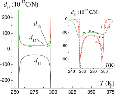
Figure 6: Piezoelectric coefficients $d_{1i}$ of Rochelle salt as functions of temperature. The inset: $d_{11}$ as a function of temperature at different fields $E_{1}$ (kV/cm): 1, 0; 2, $\bigtriangleup$: 0.304; 3, $\blacksquare$: 5. Lines: a theory; symbols: experimental points taken from [27] ($\blacksquare$) and [28] ($\bigtriangleup$).

4.4 Hydrostatic pressure effects

Below we shall discuss how the high-pressure effects are described by the proposed modification of the Mitsui model. Figure 7 shows the calculated hydrostatic pressure dependence of the Curie temperatures. The proposed theory reproduces the experimentally observed linear increase of both Curie temperatures with pressure at its low values, as well as the increase of $\partial T_{\rm C1}/\partial p_{\mathrm{h}}$ at higher pressures. The calculated slopes are 3.7 K/kbar at low pressures and 4.3 K/kbar above 12 kbar.

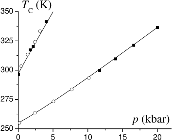
Figure 7: Hydrostatic pressure dependence of the Curie temperatures of Rochelle salt. Lines: a theory; open and closed symbols: experimental points taken from [22] and [23].

To describe the pressure variation of the static permittivity we need to make some changes in the theory parameters. The above given value of $\mu_{1}$ provides a roughly equal fit to many different experimental data for $\chi_{11}^{\sigma}$ in paraelectric phases at atmospheric pressure. However, the sample to sample variation of permittivity at ambient pressure reaches 10% even in good samples [42] and is much larger in samples with defects. This is comparable with the changes in the Curie constants produced by hydrostatic pressure [23, 9] below 10 kbar. Thus, it seems impossible to try to describe these fine high-pressure effects, using for a non-deformed crystal the averaged value of $\mu_{1}$ given in table 1. Instead, we shall determine separate values of $\mu_{1}$, which provide the best fit to the experimental data for static permittivity obtained in [23] and in [41] at each pressure considered therein. Thus, the possible pressure variation of the effective dipole moment $\mu_{1}$ can be inferred.

The measurements, reported both in [23] and in [41], revealed a decrease of the peak value of permittivity at a lower Curie temperature with increasing pressure. This is attributed [23] to a partial clamping of the samples due to the increased viscosity of the pressure-transmitting fluid and suppression of the piezoelectric shear strain $\varepsilon_{4}$. To calculate the dielectric permittivity of a partially clamped crystal we assume that the clamping caused by the viscous fluid under hydrostatic pressure is uniform throughout the crystal sample. We assume that, at least, the part of shear strain $\varepsilon_{4}$ induced by the measuring electric field (normally at 1 kHz) is smaller than the one given by equation (9). The total strain is then equal to

$$\varepsilon_{4}=\varepsilon_{s4}+k\left(\frac{e_{14}^{0}}{c_{44}^{E0}}E_{1}-\frac{2\psi_{4}}{vc_{44}^{E0}}\xi_{i}\right).$$ (23)

Here $\varepsilon_{s4}$ is a spontaneous part of the strain; $\xi_{i}$ is the field-induced part of the order parameter.

The introduced phenomenological coefficient $0<k<1$ describes the extent to which the external pressure suppresses the shear strain $\varepsilon_{4}$: the cases $k=0$ and $k=1$ correspond to the totally clamped and free crystals, respectively. Values of $k$ are, naturally, pressure and temperature dependent and are different for experimental setups with different pressure-transmitting liquids. Thus, the level of clamping at $T_{\rm C1}$ was apparently much higher in the experimental setup of [41] than in [23], possibly because the corresponding temperatures are lower, and the viscosity of pressure-transmitting liquid is higher (benzine and silicone oil [41] vs pentane isopentane mixture [23]).

Substituting equation (23) into equation (10) we obtain the corresponding polarization. Differentiating it with respect to $E_{1}$, taking into account equation (7) and neglecting variation of diagonal strains with the field, we get the dielectric susceptibility of a partially uniformly clamped crystal

$$\chi_{11}^{k}=\chi_{11}^{k0}+\frac{\beta(\mu_{1}^{k})^{2}}{2v\varepsilon_{0}}\frac{\varphi_{3}}{\varphi_{2}-k\Lambda\varphi_{3}}\,,$$ (24)

where

$$\chi_{11}^{k0}=\chi_{11}^{\varepsilon 0}+\frac{k}{\varepsilon_{0}}e_{14}^{0}d_{14}^{0}\,,\qquad\mu_{1}^{k}=\mu_{1}-2k\psi_{4}d_{14}^{0}\,.$$

From equation (24) in the limiting cases $k=0$ and $k=1$ we obtain susceptibilities of totally clamped and free (in the paraelectric phases) crystals. In the ferroelectric phase, a more accurate expression for susceptibility should also contain terms like $\sum{e_{1i}d_{1i}}$, albeit small, produced by contributions of diagonal strains. In this subsection these contributions will be neglected, and permittivity will be calculated using equation (24).

The temperature curve of dielectric permittivity near the lower Curie point at atmospheric pressure presented in [23] appears to be drawn qualitatively. In the fitting procedure we relied on the data of [3] for these temperatures. Near the upper Curie point, the data of [23] and [3] agree fairly well.

Comparison of the calculated temperature dependences of the permittivity with experimental data is given in figures 8 and 9. A fairly good description of the experiment in paraelectric phases is obtained at a proper choice of $k$ and $\mu_{1}$ values. The disagreement at 2.2 and 4.1 kbar in figure 9 is due to the mismatch between the calculated and experimental Curie temperatures at these pressures. The disagreement observed in the ferroelectric phase is due to the essential domain contributions to the permittivity, not included into the present model.

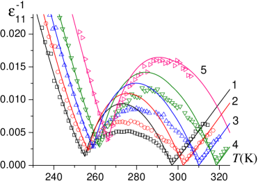
Figure 8: The temperature dependence of the inverse static permittivity of Rochelle salt at different values of hydrostatic pressure $p_{\mathrm{h}}$ (kbar): 1, $\square$: 0; 2, $\bigcirc$: 0.5; 3, $\triangle$: 1.2; 4, $\nabla$: 2; 5, $\vartriangleright$: 3.2. Lines: a theory; symbols: experimental points taken from [41].

To fit the data of [41] the coefficient $k$ is taken to be 1 at 297 K (a free crystal). At 255 K we use the following values of $k$: 0.65, 0.4, 0.25, 0.2 at 0, 0.5, 1.2, 2.0 kbar, respectively. A linear interpolation between these values at 255 K and 1 at 297 K is used. For 3.2 kbar we use $k=0$ at 265 K and 1 at 297 K, also with a linear interpolation for the intermediate temperatures. For the data of [23] we use $k=0.9$ above 11.7 kbar for the lower Curie temperature.

The pressure and temperature variation of the dipole moment $\mu_{1}$ is more complicated and contradictory. First, to fit the experimental data of [41] for permittivity at ambient pressure we have to assume that $\mu_{1}$ increases with temperature; whereas for the data of [23], [3] it should be assumed to decrease with increasing temperature, but slower than it was given in table 1.

To fit the permittivity points at high pressures we need to assume that the pressure dependence of $\mu_{1}$ is opposite to its temperature dependence: if it decreases with increasing temperature, then it increases with pressure and vice versa. Thus, for the data of [23] we use the following dependence

$$\mu_{1}=\mu_{1}^{0}\left[1+k_{\mathrm{T}}\left(T-T_{\rm C2}^{0}\right)\right]\left(1+k_{\mathrm{p}}p\right)$$

with $\mu_{1}^{0}=8.94\cdot 10^{-30}$ C$\cdot$m and $k_{\mathrm{T}}=-0.001$ K^-1. The pressure coefficient $k_{\mathrm{p}}$ was $0.03$ kbar^-1 for pressures below 5 kbar and 0 above 10 kbar.

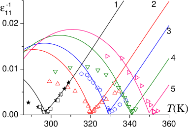
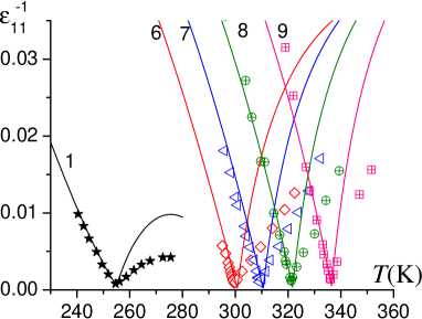
(a)

(b)

Figure 9: (Color online) The temperature dependence of the inverse static permittivity of Rochelle salt near the upper (left) and lower (right) Curie points. The values of hydrostatic pressure are: 1, $\bigstar$, $\square$: 0; 2, $\triangle$: 2.2; 3, $\bigcirc$: 3; 4, $\triangledown$ : 4.1; 5, $\vartriangleright$: 5; 6, $\diamond$: 11.6; 7, $\vartriangleleft$: 14; 8, $\bigoplus$: 16.6; 9, $\boxplus$: 20. Symbols are experimental points taken from [3] ($\bigstar$) and [23] (other symbols). Lines: a theory.

This behavior is quite unusual since the dipole moments are expected to be reduced by hydrostatic pressure or by decreasing temperature due to the overall reduction of interatomic distances. The increase of $\mu_{1}$ with hydrostatic pressure can be explained with the help of a certain assumption used in constructing the spatial four-sublattice model of Rochelle salt [44]. It states that the dipole moments in it are actually the 3D vectors, which are not oriented along the $a$-axis like in the two-sublattice model. Their projections on the $b$ and $c$ axes are different from zero, but compensated at all temperatures, unless an electric field perpendicular to spontaneous polarization is applied. The $a$-projections are the dipole moments of a two-sublattice Mitsui model, compensated in paraelectric phases. It may be assumed that hydrostatic pressure rotates the spatial dipoles in such a way that their projections on the $a$-axis (and $\mu_{1}$) increase. This increase is fast at low pressures and slows down above 10 kbar, possibly because the dipoles are already oriented along the $a$-axis.

To fit the data of [41] we use $\mu_{1}^{0}=1.0\cdot 10^{-30}$ C$\cdot$m, $k_{\mathrm{T}}=0.003$ K^-1, and $k_{\mathrm{p}}=-0.012$ kbar^-1. This is consistent with the picture when pressure and temperature affect the dipole moment $\mu_{1}$ in the opposite ways. The measurements [41] of humidity (extreme drying and wetting) effect on the permittivity of Rochelle salt have shown that in strongly wet samples the permittivity increases significantly as compared to the permittivity of normal samples, especially in the upper paraelectric phase. It appears that the samples used in the hydrostatic pressure studies [41] were moderately wet. On the other hand, a decrease of $\mu_{1}$ with increasing temperature (like in [23, 42, 3]) seems to be an intrinsic behavior of normal Rochelle salt samples. To explain the increase of $\mu_{1}$ with temperature in wet samples we can assume that due to the excess of water, the crystal conductivity increases, thus increasing the dielectric permittivity, especially at high temperatures where the mobility of charge carriers is very high.

4.5 Uniaxial pressures effects

To get a clearer picture of the uniaxial pressure effect on the Curie temperature and dielectric permittivity, it is useful to analyze it within the phenomenological approach. We start with the thermodynamic potential

$$\frac{G_{1}}{V}=-\frac{1}{2}\sum_{ij=1}^{3}s_{ij}p_{i}p_{j}-\frac{s_{44}^{P}}{2}p_{4}^{2}-P_{1}\sum_{i=1}^{3}M_{1i4}p_{i}p_{4}+g_{14}P_{1}p_{4}+P_{1}^{2}\sum_{i=1}^{3}Q_{1i}p_{i}+\frac{1}{2}\alpha P_{1}^{2}+\frac{1}{4}\beta P_{1}^{4}\,,$$

(where $s^{P}_{i4}=M_{1i4}P_{1}$ are the elastic compliances, and the $M_{1i4}$ are simply the proportionality coefficients between $s^{P}_{i4}$ and polarization. Also, $Q_{1i}$ are the electrostriction constants; $\alpha=\alpha_{\mathrm{T}}(T-T_{\rm C2}^{0})$ or $\alpha=\alpha_{\mathrm{T}}(T_{\rm C1}^{0}-T)$, $\beta$ are the coefficients of the Landau expansion). Hence, one gets the following expressions for the temperature and magnitude of the permittivity maxima

$$T^{\mathrm{max}}_{1,2}=T_{\rm C1,2}^{0}\pm\frac{2}{\alpha_{\mathrm{T}}}\sum_{i=1}^{3}Q_{1i}p_{i}+\frac{3}{4}\frac{(4\beta)^{1/3}}{\alpha_{\mathrm{T}}}\left(E_{1}-\sum_{ij=1}^{3}M_{1i4}p_{i}p_{4}+g_{14}p_{4}\right)^{2/3},$$

$$\varepsilon_{\mathrm{max}}^{-1}=\frac{3}{2}(4\beta)^{1/3}\left(E_{1}-\sum_{ij=1}^{3}M_{1i4}p_{i}p_{4}+g_{14}p_{4}\right)^{2/3}.$$ (25)

In the absence of the fields conjugate to the order parameter ($E_{1}$ and $p_{4}$), the $T^{\mathrm{max}}_{1,2}$ correspond to the phase transition temperatures. As one can see, in this approximation the uniaxial and hydrostatic ($p_{\mathrm{h}}=p_{1}=p_{2}=p_{3}$) pressures lead to linear shifts of the Curie temperatures, where the permittivity still diverges. In combination with the shear pressure $p_{4}$ they smear the transitions, shift the permittivity maxima, and lower the peaks height. It also follows from equation (4.5) that if $p_{4}=0$

$$\frac{\partial T_{{\rm C}k}}{\partial p_{\mathrm{h}}}=\sum_{j=1}^{3}\frac{\partial T_{{\rm C}k}}{\partial p_{j}}\,.$$ (26)

In table 3 we summarize the experimental data on the uniaxial pressure slopes of the transition temperatures of Rochelle salt and present our results obtained within the herein developed modification of the Mitsui model. The data of [25] are estimated from the presented therein $\varepsilon_{11}(T)$ curves, each being measured at a single value of $p_{i}$ near the upper Curie temperature.

Table 3: Uniaxial pressure derivatives of the transition temperatures of Rochelle salt (in K/kbar).

	[24]	[25]	[26]	this work
$\partial T_{\rm C1}/\partial p_{1}$	–29			–26.6
$\partial T_{\rm C1}/\partial p_{2}$	15			14.8
$\partial T_{\rm C1}/\partial p_{3}$	17			18.0
$\partial T_{\rm C1}/\partial(p_{2}+p_{3})$			$30\pm 2$	34.0
$\partial T_{\rm C2}/\partial p_{1}$	35	35.6		32.9
$\partial T_{\rm C2}/\partial p_{2}$	–16	–18		–16.5
$\partial T_{\rm C2}/\partial p_{3}$	–8	–6.7		–8.5
$\partial T_{\rm C2}/\partial(p_{2}+p_{3})$			$-22\pm 1$	–26.2

The theory and experiment for the uniaxial pressures agree within 10%, which is close to the experimental error [24]. The theoretical dependence of the Curie temperatures on the biaxial pressure $p_{2}+p_{3}$ is a little stronger than the experimental one. Also it can be noticed that equation (26) is not fulfilled.

Independent measurements [26, 41, 25] of dielectric susceptibility of Rochelle salt under different uniaxial and biaxial pressures revealed a decrease of the peak values of susceptibility at the Curie points as well as smearing out of the peaks. These effects are enhanced with increasing pressures.

A uniform partial clamping of samples by an apparatus creating the uniaxial pressures can explain the observed lowering of the peaks, but not the smearing of the transitions. As an intrinsic phenomenon, both these effects can be caused by application of an external field conjugate to the order parameter: the electric field $E_{1}$ directed along the axis of spontaneous polarization or the shear stress $\sigma_{4}$, that is, by the field which induces polarization $P_{1}$ in the paraelectric phases. In an ideal experiment, no uniaxial or biaxial pressure applied along the orthorhombic crystallographic axes should act in this way, because piezoelectric coefficients associated with these pressures are zeros outside the ferroelectric phase.

It appears that the observed smearing of the anomalies is an artefact caused by experimental errors. We can think of the following factors that in a real experiment can lead to the smearing.

• Stress inhomogeneity. Even a weak inhomogeneity of the applied pressure, partial clamping/sample end constraints, surface irregularity result in a non-uniform strain distribution over the crystal sample; thus, in different parts of the sample the phase transition is shifted to different temperatures. The higher is pressure, the larger is the difference between these temperatures, and the more diffuse is the transition, exactly as observed in [41].

• Stray shear stress $\sigma_{4}$, whose effect would be enhanced by its combination with the uniaxial pressures $p_{i}$, as it follows from equation (4.5). The stress $\sigma_{4}$ can arise even at a slight misorientation of the samples, as a component of the uniaxial loading intended to create $p_{2}$ or $p_{3}$ pressures. There can also occur built-in local shear stresses $\sigma_{4}$ caused by sample defects, e.g. dislocations.

There will be too much uncertainty if we try to take the effect of these factors into account in the theory. Thus, we shall not attempt to describe the behavior of the static dielectric susceptibility in uniaxially stressed Rochelle salt crystals.

5 Concluding remarks

We proposed a generalization of the deformable Mitsui model [9], which along with the piezoelectric shear strain $\varepsilon_{4}$ takes into account the diagonal strains $\varepsilon_{1}$, $\varepsilon_{2}$, and $\varepsilon_{3}$ as well. In contrast to the previous attempt [19], in order to incorporate the diagonal strains into this model, the thermal expansion is consistently taken into account.

In the mean field approximation we find polarization and the strains, as well as thermal, elastic, and piezoelectric characteristics related to diagonal strains. For the case of Rochelle salt we suggest an elaborated fitting procedure and choose the set of the model parameter values, providing as good as possible consistent description of all these characteristics, as well as of external hydrostatic and uniaxial pressure effects.

The expression for susceptibility of a partially clamped crystal is derived in order to describe the behavior of the observed susceptibility of Rochelle salt under hydrostatic pressure near the lower Curie point. By fitting the theoretical curves to the experimental points, the pressure variation of the effective dipole moment $\mu_{1}$ is estimated. An increase of $\mu_{1}$ with hydrostatic pressure at low pressures and a decrease with increasing temperature seem to be an intrinsic behavior for this crystal. The interaction constants and the asymmetry parameter were found to increase with hydrostatic pressure too. This is consistent with the picture, where the dipole moments in Rochelle salt are 3D vectors [44], assuming they rotate under pressure in such a way that their projection on the $a$-axis increases.

Apart from Rochelle salt, the developed modification of the model with appropriate changes can be used for consideration of the pressure effects and thermal expansion in other ferroelectric crystals described by the Mitsui model. The fitting procedure, however, for each such crystal will require extensive experimental data; further measurements will, therefore, be necessary.

The presented model and the found values of its parameters are a good starting point for developing a model description of ferroelectricity in nanosize inclusions of compounds, to which the Mitsui model is applicable, grown in a porous matrix [11, 13, 14].

Модель Мiцуї з дiагональними деформацiями: об’єднаний опис впливу зовнiшнiх тискiв i теплового розширення в сеґнетовiй солi NaKC₄H₄O${}_{6}\cdot 4$H₂O А.П. Моїнаlabel1, Р.Р. Левицькийlabel1, I.Р. Зачекlabel2

label1Iнститут фiзики конденсованих систем НАН України, 79011 Львiв, вул. Свєнцiцького, 1 label2 Нацiональний унiверситет “Львiвська полiтехнiка”, 79013 Львiв, вул. С. Бандери, 12

References

- [1] Mitsui T., Phys. Rev., 1958, 111, 1259; \bibdoi10.1103/PhysRev.111.1259.
-
[2]
Vaks V.G., Zinenko V.I., Schneider V.E., Sov. Phys. Uspekhi, 1983, 26, 1059;
\bibdoi10.1070/PU1983v026n12ABEH004584. -
[3]
Schneider U., Lunkenheimer P., Hemberger J., Loidl A.,
Ferroelectrics, 2000, 242, 71;
\bibdoi10.1080/00150190008228404. - [4] Aleksandrov K.S., Anistratov A.T., Ferroelectrics, 1976, 12, 191; \bibdoi10.1080/00150197608241423.
- [5] Blat D.Kh., Zinenko V.I., Fiz. Tverd. Tela (Leningrad), 1976, 18, 3599.
- [6] Watarai S., Matsubara T., J. Phys. Soc. Jpn., 1978, 45, 1807; \bibdoi10.1143/JPSJ.45.1807.
- [7] Watarai S., Matsubara T., Sol. State Comm., 1980, 35, 619; \bibdoi10.1016/0038-1098(80)90595-5.
- [8] Korynevskii N.A., Ferroelectrics, 2002, 268, 207; \bibdoi10.1080/00150190211058.
-
[9]
Levitskii R.R., Zachek I.R., Verkholyak T.M., Moina A.P., Phys. Rev. B, 2003, 67, 174112;
\bibdoi10.1103/PhysRevB.67.174112. -
[10]
Moina A.P., Levitskii R.R., Zachek I.R., Phys. Rev. B, 2005,
71, 134108;
\bibdoi10.1103/PhysRevB.71.134108. - [11] Yadlovker D., Berger S., Phys. Rev. B, 2005, 71, 184112; \bibdoi10.1103/PhysRevB.71.184112.
- [12] Yadlovker D., Berger S., J. Electroceram., 2007, 22, 281.
- [13] Baryshnikov S.V., Charnaya E.V., Stukova E.V., Milinskii A.Yu., Cheng Tien, Fiz. Tverd. Tela, 2010, 52, 1347 [Phys. Solid State 52, 1444 (2010); \bibdoi10.1134/S1063783410070206].
- [14] Cheng Tien, Charnaya E.V., et al., J. Phys.: Condens. Matter, 2008, 20, No. 21, 215205; \bibdoi10.1088/0953-8984/20/21/215205.
- [15] Niznansky D., Plocek J., Svobodova M., Nemec I., Rehspringer J.-L., Vanek P., Micka Z., J. Sol-Gel Sci. Technol., 2003, 26, 447; \bibdoi10.1023/A:1020702005541.
-
[16]
Morozovska A.N., Eliseev E.A., Glinchuk M.D., Phys. Rev. B, 2006, 73, 214106;
\bibdoi10.1103/PhysRevB.73.214106. - [17] Levitskii R.R., Moina A.P., Andrusyk A.Ya., Slivka A.G., Kedyulich V.M., J. Phys. Stud., 2008, 12, 2603.
- [18] Lipinski I.E., Kuriata J., Korynevskii N.A., Ferroelectrics, 2005, 317, 115.
- [19] Levitskii R.R., Zachek I.R., Moina A.P., Condens. Matter Phys., 2005, 8, 881.
- [20] Suzuki E., Shiozaki Y., Phys. Rev. B, 1996, 53, 5217; \bibdoi10.1103/PhysRevB.53.5217.
-
[21]
Hlinka J., Kulda J., Kamba S., Petzelt J., Phys. Rev. B, 2001, 63, 052102;
\bibdoi10.1103/PhysRevB.63.052102. - [22] Bancroft D., Phys. Rev., 1938, 53, 587; \bibdoi10.1103/PhysRev.53.587.
- [23] Samara G.A., J. Phys. Chem. Solids, 1965, 26, 121; \bibdoi10.1016/0022-3697(65)90079-X.
- [24] Imai K., J. Phys. Soc. Jpn., 1975, 39, 868; \bibdoi10.1143/JPSJ.39.868.
- [25] Unruh H.-G., Müser H.E., Ann. Phys., 1967, 474, 28; \bibdoi10.1002/andp.19674740105.
- [26] Mori K., Hayashi M., J. Phys. Soc. Jpn., 1972, 33, 1396; \bibdoi10.1143/JPSJ.33.1396.
- [27] Schmidt G., Z. Angew. Phys., 1961, 161, 579; \bibdoi10.1007/BF01341554.
- [28] Fotchenkov A.A., Sov. Phys. Crystallogr., 1960, 5, 390.
- [29] Sailer E., Unruh H.-G., Ferroelectrics, 1976, 12, 285; \bibdoi10.1080/00150197608241452.
-
[30]
Wlodarz M., Bronowska W., Dziedzic J., Ferroelectr. Lett., 1988,
9, 83;
\bibdoi10.1080/07315178808200706. - [31] Imai K., J. Phys. Soc. Jpn., 1976, 41, 2005; \bibdoi10.1143/JPSJ.41.2005.
- [32] Numerical Data and Functional Relationships in Science and Technology, eds. Hellwege K.-H. and Hellwege A.M. Landolt-Bornstein, New Series. Group III: Crystal and Solid State Physics, Vol. 16, Pt. b. Springer-Verlag, Berlin, 1982.
- [33] Anderson P.W., Halperin B.I., Varma C.M., Philos. Mag., 1972, 25, 1; \bibdoi10.1080/14786437208229210.
- [34] Phillips W.A., J. Low Temp. Phys., 1972, 7, 351; \bibdoi10.1007/BF00660072.
- [35] Bronowska W.J., J. Appl. Crystallogr., 1981, 14, 203; \bibdoi10.1107/S0021889881009114.
- [36] Vaks V.G., Introduction into Microscopic Theory of Ferroelectrics. Nauka, Moscow, 1973 (in Russian).
- [37] Levitskii R.R., Verkholyak T.M., Kutny I.V., Hil I.G. Preprint arXiv:cond-mat/0106351 (unpublished).
- [38] Dublenych Yu.I., Condens. Matter Phys., 2011, 14, 23603; \bibdoi10.5488/CMP.14.23603.
- [39] Berlincourt D.A., Curran D.R., Jaffe H. – In: Physical Acoustics, Vol. 1, Part A, p. 169–270, ed. W.P. Mason. Academic Press, New York, 1964.
- [40] dos Santos A., de Menezes A.S., Sasaki J.M., Cardoso L.P., Acta Crystallogr., Acta Crystallogr., Sect. A: Found. Crystallogr., 2008, 64, C544.
- [41] Slivka A.G., Kedyulich V.M., Levitskii R.R., Moina A.P., Romanyuk M.O., Guivan A.M., Condens. Matter Phys., 2005, 8, 623.
- [42] Sandy F., Jones R.V., Phys. Rev., 1968, 168, 481; \bibdoi10.1103/PhysRev.168.481.
- [43] Tatsumi M., Matsuo T., Suga H., Seki S., J. Phys. Chem. Solids, 1978, 39, 427; \bibdoi10.1016/0022-3697(78)90084-7.
- [44] Stasyuk I.V., Velychko O.V., Ferroelectrics, 2005, 316, 51; \bibdoi10.1080/00150190590963138.