Partner Selection
in Indoor-to-Outdoor Cooperative Networks:
an Experimental Study

Abstract

In this paper, we develop a partner selection protocol for enhancing the network lifetime in cooperative wireless networks. The case-study is the cooperative relayed transmission from fixed indoor nodes to a common outdoor access point. A stochastic bivariate model for the spatial distribution of the fading parameters that govern the link performance, namely the Rician K-factor and the path-loss, is proposed and validated by means of real channel measurements. The partner selection protocol is based on the real-time estimation of a function of these fading parameters, i.e., the coding gain. To reduce the complexity of the link quality assessment, a Bayesian approach is proposed that uses the site-specific bivariate model as a-priori information for the coding gain estimation. This link quality estimator allows network lifetime gains almost as if all K-factor values were known. Furthermore, it suits IEEE 802.15.4 compliant networks as it efficiently exploits the information acquired from the receiver signal strength indicator. Extensive numerical results highlight the trade-off between complexity, robustness to model mismatches and network lifetime performance. We show for instance that infrequent updates of the site-specific model through K-factor estimation over a subset of links are sufficient to at least double the network lifetime with respect to existing algorithms based on path loss information only.

I Introduction

Wireless sensor networks (WSN) are the enabling technology for home and building automation [1, 2]. The main obstacle in the development of WSNs is the cost of battery replacement, which becomes even more pronounced for indoor-to-outdoor (I2O) communication with its larger transmit powers requirements. In this paper we aim at designing a medium access control (MAC) protocol for I2O WSNs that minimizes the maximum transmit energy so as to prolong the network lifetime [3].

Transmit energy can be reduced by implementing advanced cooperative relaying strategies [4], that efficiently exploit the inherent spatial diversity of a distributed radio channel. Selecting the partner for each node [5] is the most crucial task in the coordination phase of any cooperative technique [6]. Partner selection is either based on instantaneous or average channel quality indicators of the links [7, 8]. Additional knowledge on macroscopic features such as the network topology [9] and a parametric characterization of the fading channel, e.g., a path-loss model [10], can be also exploited.

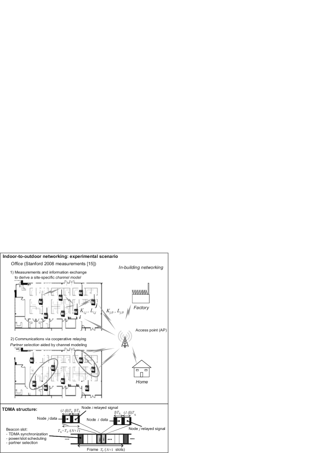
Figure 1: Top: general indoor networking scenario and the specific I2O office radio measurement plan in [15]; indoor nodes are allowed to support the estimation of a site-specific stochastic channel model (1), and to engage in cooperative transmission to the access point (2). Bottom: TDMA framing structure inspired to the IEEE 802.15.4 beacon mode.

In this paper we focus on the transmission from several indoor static nodes in a single-floor office or factory to a common outdoor access point (AP), as outlined in Fig. 1 (top). Nodes are permitted to engage in cooperative transmissions by amplifying and forwarding (AF) [11] the signals received from the partner nodes. We are interested to develop a partner selection scheme that maximizes the network lifetime under reliability and rate constraints that are identical for all nodes. We propose an original approach where the partner selection is aided by the knowledge of a site-specific multi-link stochastic channel model. The network employs a time division multiple access (TDMA) scheme inspired by the IEEE 802.15.4 access protocol in “beacon mode” [12], as depicted in Fig. 1 (bottom).

In [7] selection cooperation based on instantaneous channel state information (CSI) has been introduced. For large networks such an approach requires the exchange of large amounts of CSI within the coherence time of the fading channel. To reduce the transmission overhead, here we are interested to employ long-term channel properties for the partner selection stage. This approach has been used by the pairing protocol in [8], which is based on the path loss values. This is a very practical choice, as e.g. in the IEEE 802.15.4 standard a received signal strength indicator (RSSI) is available [13]. However, an indication of the randomness of the fading is also required for assessing the quality of a link. This randomness can be assessed by the Rician K-factor, as shown by physical fading channel modeling [14].

Contributions of this work

(i) We design a MAC protocol where the AP assigns the partner and transmission resources to each node based on information about the path loss and the Rician K-factor, extending the method of [8]. For this protocol we provide a performance assessment in terms of network lifetime, utilizing realistic I2I/I2O channel models.

(ii) We propose an empirical, but analytically tractable, stochastic model for the characterization of the two fading parameters, namely, the path loss and the Rician K-factor for the links in an indoor network with fixed nodes. The two parameters are modeled jointly generalizing existing scalar models, e.g., [14]. The so-called bivariate channel model is drawn and validated using the multi-link channel measurement data [15].

(iii) For low-power operation of a cooperative WSN, we propose a procedure where (1) the K-factor is estimated on a small number of nodes with a slow update cycle: this distributed information is conveyed to the central coordinator in order to update the bivariate model parameters; (2) the estimation of the link-quality for each transmission is based on the local average RSSI and the regularly updated bivariate channel model as common a priori information. We compare the performance of this approach with the one where both the path-loss and the K-factor are permanently re-estimated for each transmission.

II System Model

The scenario under study consists of $N$ battery-powered indoor nodes that communicate with a common AP located outdoors. The nodes transmit during a communication session. In each session, the AP is acting as the centralized coordinator for assigning the cooperating partners, configuring the time-slot assignments and radio-frequency (RF) transmit powers. Complex base-band notation is used to model the wireless link between node $i\in\{1,\ldots,N\}$ and node $j\in\{0,\ldots,N\}$, with node $j=0$ referring to the AP. The received signal at node $j$ is $y_{i,j}=h_{i,j}x_{i}+n_{j}$ where $h_{i,j}$ is the frequency-flat complex channel coefficient, $x_{i}$ is the symbol transmitted by node $i$ with transmit power $\rho_{i}$, $n_{j}$ is additive symmetric complex white Gaussian noise with variance $\sigma^{2}$. The instantaneous signal-to-noise ratio (SNR) for from node $i$ to $j$ is modeled as

$$\gamma_{i,j}=\left(\rho_{i}/\sigma^{2}\right)\left|h_{i,j}\right|^{2}.$$ (1)

The square fading envelope $\left|h_{i,j}\right|^{2}$ is constant for the whole codeword duration (block fading) and varies from codeword to codeword according to the Rician distribution [16], such that $L_{i,j}=-\left(\mathbb{E}\left[\left|h_{i,j}\right|^{2}\right]\right){}_{\mathrm{dB}}$ denotes the path loss in dB and $K_{i,j}=\left(\left|\mathbb{E}\left[h_{i,j}\right]\right|^{2}\right){}_{\mathrm{dB}}-\left(\mathrm{var}\left[h_{i,j}\right]\right){}_{\mathrm{dB}}$ denotes the Rician K-factor in dB. The term path loss, used for indicating $L_{i,j}$, includes the large-scale shadow fading and the static component of the small-scale fading as detailed in Sect. III-A. The block fading assumption motivates the use of outage probability and it is confirmed by channel measurements (see [15]).

II-A Medium Access Control and Node Coordination

The transmission is organized into frames of duration $T_{\mathrm{F}}$, further divided into $N+1$ subframes for time division multiple access (TDMA), as shown in Fig. 1 (bottom). A unique subframe of duration $T_{\mathrm{S}}=T_{\mathrm{F}}/(N+1)$ is assigned to each node by the AP. The AP also provides the reference clock to all the nodes, the grouping decisions and access coordination (e.g., power and time slots allocation) through a periodic beacon transmission [12].

Let $\left(i,j\right)$ be a pair of cooperating nodes, to accommodate cooperative transmission each subframe assigned to any of these two nodes is further subdivided into two slots. As depicted in Fig. 1, for node $i$ the first slot spans a fraction $\beta_{i}=\beta$ of the subframe duration and it is used to transmit the node $i$ data. The second slot with duration $\left(1-\beta_{i}\right)T_{\mathrm{S}}=\left(1-\beta\right)T_{\mathrm{S}}$ is reserved for helping the assigned partner node $j$. In a specular way, the first and second slots of the subframe assigned to node $j$ span, respectively, the fractions $\beta_{j}=1-\beta$ (for node-$j$ data) and $\left(1-\beta_{j}\right)=\beta$ (for forwarding node-$i$ data). The AP optimally combines the noisy replicas of the signals coming from the two nodes for data detection.

II-B Outage Probability Modeling

For point-to-point transmission the outage probability is $P_{\mathrm{out}}^{\textrm{dir}}=\Pr[\gamma_{i,j}<\gamma_{\mathrm{th}}^{\mathrm{dir}}],$ where the SNR threshold $\gamma_{\mathrm{th}}^{\mathrm{dir}}=\left(2^{R}-1\right)/\Gamma$ , $R$ is the spectral efficiency measured in bit/channel use. The gap $0\leq\Gamma\leq 1$ can be varied by changing modulation/coding format and targeted bit error rate (BER) level (see [17] and references therein). The outage probability is assessed according to the models in [18], here adapted to the considered scenario.

For the Rician fading model, the outage probability for node $i$ communicating directly with any node $j$ can be parametrized in terms of the so-called coding gain $c_{i,j}$

$$P_{\mathrm{out}}^{\textrm{dir}}\approx\frac{\gamma_{\mathrm{th}}^{\mathrm{dir}}\sigma^{2}}{c_{i,j}\rho_{i}}\text{,}$$ (2)

where $\approx$ indicates that the equality holds asymptotically for high SNR. The coding gain $c_{i,j}$ depends on the K-factor $K_{i,j}$ and the path loss $L_{i,j}$ according to:

$$c_{i,j}=\frac{e^{\theta(K_{i,j})}}{\theta\left(L_{i,j}\right)\left[1+\theta\left(K_{i,j}\right)\right]}.$$ (3)

For convenience of notation we introduce the function $\theta(\cdot)=10^{(\cdot)/10}$ with inverse $\theta^{-1}(\cdot)=10\log_{10}(\cdot)$ (recall that $K_{i,j}$ and $L{}_{i,j}$ have been defined in dB).

To model the performance of cooperative transmission of node $i$ with the help of node $j$ (here $j\neq 0$), we consider the AF relaying scheme as it has a simple architecture that facilitates practical implementation. Node $j$ periodically overhears the signal transmitted by the partner node $i$ and amplifies-and-forwards it towards the AP [11]. The amplification is based on a variable gain approach, where the power amplification gain $a_{j}=\rho_{j}/\left[\sigma^{2}(\gamma_{i,j}+1)\right]$ is dynamically adjusted to the instantaneous SNR $\gamma_{i,j}$. Note that the node must maintain a constant transmit power $\rho_{j}$ for the whole assigned subframe, i.e. also during the relaying phase, so as to avoid amplifier non-linearities by switching the power level. Recalling that the AP optimally combines the two noisy replicas of the source signal, the effective SNR

$$\gamma_{(i,j),0}=\gamma_{i,0}+\left(\frac{1}{\gamma_{i,j}}+\frac{1}{\gamma_{j,0}}+\frac{1}{\gamma_{i,j}\gamma_{j,0}}\right)^{-1}.$$ (4)

The outage probability for cooperative transmission

$$P_{\mathrm{out}}^{\mathrm{coop}}=\Pr[\gamma_{(i,j),0}<\gamma_{\mathrm{th}}^{\mathrm{coop}}]\approx\frac{1}{2}\left(\frac{\gamma_{\mathrm{th}}^{\mathrm{coop}}\sigma^{2}}{c_{(i,j),0}\rho_{(i,j),0}}\right)^{d_{(i,j),0}},$$ (5)

with $\gamma_{\mathrm{th}}^{\mathrm{coop}}=\left(2^{R/\beta_{i}}-1\right)/\Gamma$. The spectral efficiency $R$ is now multiplied by $1/\beta_{i}$ to guarantee the same efficiency as for the non-cooperative case. Notice that this assumption implies that the low-power radio transceiver is designed to support multiple data rates [19]. Also, we select the same gap $\Gamma$ for all rates. Terms $\rho_{(i,j),0}$, $c_{(i,j),0}$ and $d_{(i,j),0}$ denote the effective power, coding gain, and diversity order for the cooperative link $(i,j),0$, respectively. For Rician fading, it is $d_{(i,j),0}=2$, $\rho_{(i,j),0}=\sqrt{\rho_{i}\rho_{j}}$ , and

$$c_{(i,j),0}=\left[\frac{1}{c_{i,0}}\left(\frac{1}{c_{i,j}}+\frac{1}{c_{j,0}}\right)\right]^{-\frac{1}{2}},$$ (6)

where the coding gains depend on the K-factors and the path loss values, as in (3).

II-C Energy Consumption Modeling

The transmit power is designed so that the outage probability at the AP is lower or equal to $p$. The corresponding energy consumption for node $i$ during one frame is derived below.

No-cooperation – From (2), the transmit power at node $i$ scales as

$$\rho_{i}\approx\frac{\gamma_{\mathrm{th}}^{\mathrm{dir}}\sigma^{2}}{c_{i,0}}\frac{1}{p}.$$ (7)

The average energy expenditure for node $i$ can thus be modeled as

$$E_{i}=\rho_{i}T_{\text{S}}+E_{\text{RX}}\frac{T_{\text{S}}}{T_{\mathrm{F}}}+E_{\text{P}},$$ (8)

where $E_{\text{RX}}$ is the energy consumption for receiving during the beacon slot only, and $E_{\text{P}}$ is the energy consumption for basic processing.

AF cooperation – For a small enough outage probability $p$, it can be shown that the minimum transmit power levels for paired nodes $(i,j)$ are

$$\rho_{i}=\rho_{j}=\rho_{(i,j),0}=\kappa(\hat{\mathrm{\beta}})\sigma^{2}/\sqrt{2p},$$ (9)

with $\kappa(\beta)=\max\left[\left(2^{R/\beta}-1\right)/\left(\Gamma c_{\left(i,j\right),0}\right),\>\left(2^{R/(1-\beta)}-1\right)/\left(\Gamma c_{\left(j,i\right),0}\right)\right]$. The subframe fraction $\beta$ for the $i$-th node message is selected so as to minimize $\rho_{(i,j),0}$:

$$\hat{\beta}\approx\frac{1}{2}-\frac{\log_{2}(\lambda)}{8R},$$ (10)

with $\lambda=\sqrt{\frac{1+c_{i,0}/c_{i,j}}{1+c_{j,0}/c_{i,j}}}$ . The notation $\approx$ indicates that the scaling law is valid for $\log_{2}(\lambda)\ll R$ (i.e., $\lambda\simeq 1$). The proofs of (9) and (10) are given in Appendix A.

Notice that using (10) for $\lambda>1$ (i.e., $c_{i,0}>c_{j,0}$), then $\hat{\beta}<1/2$ as the largest slot is reserved for helping the partner $j$ that experiences more severe fading conditions. On the other hand, if $c_{i,j}\gg\max\left[c_{i,0},\,c_{j,0}\right]$, the slots have equal length, $\hat{\beta}\approx 1/2$. Notice that the choice $\beta=1/2$ is relevant also because it models a practical system optimized for two data rates [19], i.e., the lower for no-cooperation and the higher for cooperation.

The average consumed energy for node $i$ cooperating with partner $j$ is then

$$E_{(i,j),0}^{\mathrm{AF}}=\rho_{(i,j),0}T_{\text{\text{S}}}+E_{\text{RX}}(2-\beta)\frac{T_{\text{S}}}{T_{\mathrm{F}}}+(1+\upsilon_{\text{AF}})E_{\text{P}},$$ (11)

with $\upsilon_{\text{AF}}>0$ accounting for the energy consumption for the partner signal amplification. The transmit power $\rho_{(i,j),0}$ for source and relay nodes are chosen as in (9).

III Wireless Channel Characterization

In this section we present a framework for modeling and estimating channel quality metrics for the links of the cooperative network. The final aim is to provide metrics to be used at the MAC layer for relay selection.

In Sect. III-A we propose a stochastic general model of the two fading parameters $(L_{i,j},K_{i,j})$, which includes as particular cases some models previously proposed in the literature (see e.g. [14, 20]). In Sect. III-B, the model is validated and discussed using experimental data collected by an I2I/I2O measurement campaign, with indoor nodes deployed over an office environment. The study will also provide a reliable simulation environment for assessing the performance of partner selection algorithms in Sect. V. Given the a-priori knowledge of the model, in Sect. III-C we propose a Bayesian method for the estimation of the coding gain $c_{i,j}$ starting from the path loss observation.

III-A Bivariate Model for the Large-Scale Fading Parameters

We consider a fading channel $h_{i,j}$ between any two nodes $\left(i,j\right)$ of the static network. Link indexes $\left(i,j\right)$ will be omitted when not needed, to simplify the notation. It is important to highlight that, differently from mobile scenarios, here the deterministic channel gain $\mu_{h}=E\left[h_{i,j}\right]$ accounts for the effects of fixed scattering/absorbing objects which determine the so-called static multipath component. On the other hand, temporal fading - with variance $\mathrm{\sigma_{h}^{2}=var}\left[h_{i,j}\right]$ - is due only to some moving scatterers/absorbers in the environment. As assumed in Sect. II, this results in a Rician distribution with parameters $L=-\theta^{-1}(\sigma_{h}^{2}+|\mu_{h}|^{2})$ and $K=\theta^{-1}(|\mu_{h}|^{2}/\sigma_{h}^{2})$ (recall that $\theta(\cdot)$ is the inverse of the transformation to dB). The multipath configuration changes rapidly with the node locations, thus leading to fast variations of the Rician factor $K$ and the path-loss $L$ over the space. The objective of this section is the definition of a model to describe the variations of such parameters from link to link.

Let $\mathbf{x}=[K\,\,L]^{\textrm{T}}$ be the vector collecting the two fading parameters for a generic link. We model the variations of $\mathbf{x}$ according to a bivariate Gaussian random variable (bivariate model). We assume that $\mathbf{x}$ is Gaussian distributed, $\mathbf{x}\sim\mathcal{N}\left(\mu_{\mathrm{\mathbf{x}}},\mathbf{C}\right)$, with a mean $\mu_{\mathrm{\mathbf{x}}}(D)=[\mu_{\mathrm{K}}(D)\,\,\mu_{\mathrm{L}}(D)]^{\mathbf{\mathsf{\textrm{T}}}}$ depending on the link distance $D$ and a spatially invariant covariance matrix

$$\mathbf{C}=\mathbb{\left[\begin{array}[]{cc}\mbox{$\textrm{$\sigma_{\mathrm{K}}^{2}$}$}&\varphi\sigma_{\mathrm{K}}\mbox{$\sigma_{L}$}\\ \varphi\mbox{$\sigma_{\mathrm{K}}$\mbox{$\sigma_{L}$}}&\mbox{$\sigma_{L}^{2}$}\end{array}\right]},$$ (12)

The correlation coefficient $\varphi=\mathbb{E}\left[\left(K-\mu_{\mathrm{K}}(D)\right)\left(L-\mu_{\mathrm{L}}(D)\right)\right]/(\sigma_{\mathrm{K}}\mbox{$\sigma_{L}$})$ models the mutual dependence between the K-factor and the path loss experienced over the same link. A metric, that will be relevant in partner selection analysis in Sect. IV, is the probability density function (pdf) of the K-factor conditioned on the path loss, $\mathrm{p}\left(K|L\right)=\mathcal{N}(\mu_{\mathrm{K|L}},\mbox{ }\sigma_{\mathrm{K|L}}^{2})$, with mean

$$\mu_{\mathrm{K|L}}\mathrm{\mathbb{=E}}\left[K|L\right]=\mu_{\mathrm{K}}(D)+\frac{\textrm{$\sigma_{\mathrm{K}}$}}{\sigma_{\mathrm{L}}}\varphi\left(L-\mu_{\mathrm{L}}(D)\right)$$ (13)

and variance $\mbox{ }\sigma_{\mathrm{K|L}}^{2}=\mathrm{var}\left[K|L\right]=(1-\varphi^{2})\sigma_{\mathrm{K}}^{2}.$

The parameters of the bivariate model can be tuned for different propagation scenarios, e.g. I2I and I2O, as done in the following.

III-B Experimental Calibration of the Bivariate Model and Analysis of Spatial Coherence

In this section, we describe the calibration of the model parameters $\mathbf{\mathbf{\mu}}_{\mathbf{x}}(D)$ and $\mathbf{C}$ on the I2I and I2O propagation scenarios in Fig. 1. We use the multi-link channel measurements [15] at 2.45 GHz, but also existing models whenever the data is not sufficient. It is important to mention that the fading in the experiment is caused not only by walking people but also by moving metallic objects. This contributes to determine harsh I2O propagation conditions. The 70 MHz band of the channel is divided into 60 subbands, each corresponding to a flat fading subchannel. As mentioned in Sect. III-A, in contrast to mobile scenarios, the small-scale temporal fading has a different origin compared to the small-scale fading in the spatial and spectral domains. Hence, $K_{i,j}$ and $L_{i,j}$ are estimated independently in each subband.

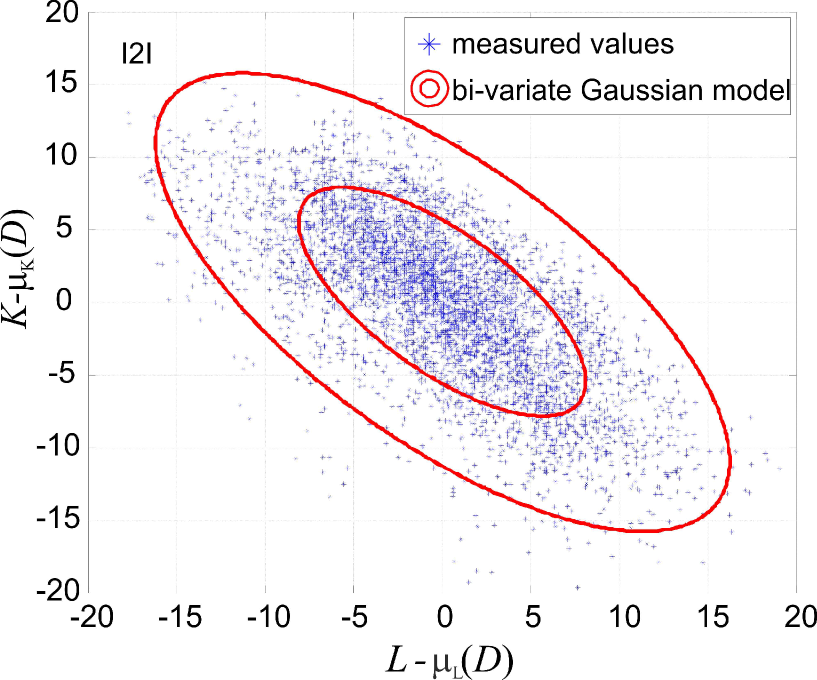
Figure 2: Measured I2I path loss and K-factor values minus the respective distance-dependent means. The equidensity contours of the zero-mean bivariate Gaussian distribution are depicted at one and two standard deviations from the mean, containing 62% and 98% of the points respectively.

I2I channel model – The vector function $\mathbf{\mathbf{\mu}}_{\mathbf{x}}(D)$ is estimated by performing linear least squares regressions of $K$ and $L$ over the corresponding distances $D$ in logarithmic scale. The covariance $\mathbf{C}$ is then obtained by computing variances and covariances on the sets of data $\left\{K-\mu_{\mathrm{K}}(D)\right\}$ and $\left\{L-\mu_{\mathrm{L}}(D)\right\}$. The $l_{\infty}$ norm of the error between the theoretic cumulative density function (cdf) of $\left\{K-\mu_{\mathrm{K}}(D)\right\}$ and $\left\{L-\mu_{\mathrm{L}}(D)\right\}$ and the empirical one is 0.04, showing a very good fit. This is apparent in Fig. 2, where the equidensity contour lines of the bivariate distribution of $(K-\mu_{\mathrm{K}}(D),L-\mu_{\mathrm{L}}(D))$ are shown together with the respective measured values.

I2O channel model – According to the urban micro-cell scenario B4 in [21], the propagation on the link $\left(i,0\right)$ is modeled as the combination of three main contributions: (i) the indoor propagation from the node to the nearest wall to the BS $\left(i\mathrm{,Wall}\right)$; (ii) the propagation through the wall; (iii) the outdoor propagation from the wall to the BS $\left(\mathrm{Wall}\mathrm{,0}\right)$. The overall link path loss $L_{i,0}$ and K-factor $K_{i,0}$ are modeled as

$$L_{i,0}=L_{i\mathrm{,Wall}}+L_{\mathrm{Wall}}+L_{\mathrm{Wall}\mathrm{,0}},\;\;K_{i,0}=K_{i\mathrm{,Wall}}+K_{\mathrm{Wall}\mathrm{,0}}.$$ (14)

Notice that the wall contribution has no effects on $K_{i,0}$. The value chosen for the wall contribution is $L_{\mathrm{Wall}}=14\mathrm{dB}$ (neglecting the angle of the propagation path with respect to the wall [21]). The specific value will not affect the performance comparison of the algorithms presented in Sect. V. The outdoor parameters $\left(L_{\mathrm{Wall}\mathrm{,0}},K_{\mathrm{Wall}\mathrm{,0}}\right)$ modeling adheres to [20, (4) and (9)]. The indoor parameter $L_{i\mathrm{,Wall}}$ is modeled according to [21, Table 4-4]. The bivariate model $(L_{i\mathrm{,Wall}},K_{i\mathrm{,Wall}})$ and the corresponding indoor correlation value are obtained by a simple manipulation of the model for $L_{i\mathrm{,Wall}}$ in [21, Table 4-4], using the line slope and the error variance of the least squares linear regression of $K$ over the corresponding $L$ in the available I2O measurements. Numerical details are provided in Table 1.

The normal distribution of $K\mid L$ has been assumed by several studies in the literature (see, e.g., [20, 16, 14]) to model the residuals of the linear least square regression of $K$ over $L$. Here, instead, we have directly tested the bivariate normal distribution of $\left\{K-\mu_{\mathrm{K}}(D)\right\}$ and $\left\{L-\mu_{\mathrm{L}}(D)\right\}$ via a 2-D fitting of the cdf. In this way, we have also highlighted the strong (negative) correlation between $\left\{K-\mu_{\mathrm{K}}(D)\right\}$ and $\left\{L-\mu_{\mathrm{L}}(D)\right\}$, also observed experimentally in our study (see the values detailed in Table 1). In contrast to line-of-sight mobile scenarios, in our case the static multipath component in $\mu_{h}$ mainly contributes to the negative correlation $\varphi$. Consider e.g. two links $(i,j_{1})$ and $(i,j_{2})$, with nodes $j_{1}$ and $j_{2}$ closely located, i.e., with distance in the order of the carrier wavelength $\lambda$ ($D_{i,j_{1}}\approx D_{i,j_{2}}$). Even if the two links are likely to experience the same channel shadowing, average fading conditions $\mu_{\mathrm{\mathbf{x}}}(D)$, and degree of temporal variations $\mathrm{\sigma_{h}^{2}}$, the two links still experience different multipath configurations and thus different values for the static multipath component in $\mu_{h}$. The variation on $\mu_{h}$ affects with opposite sign the path-loss and the K-factor, thus, a strong negative correlation is observed.

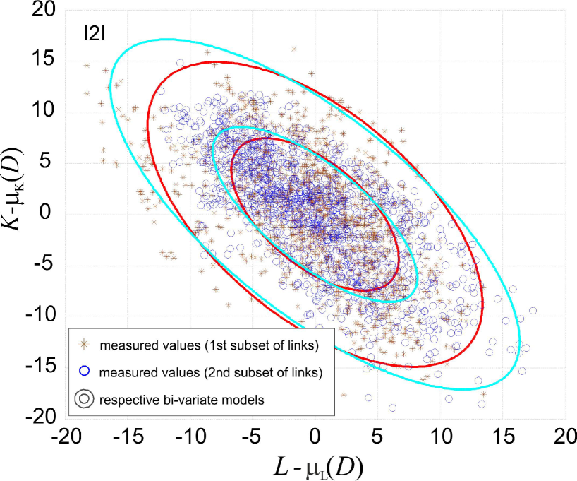
Figure 3: Measured I2I path loss and K-factor values minus the respective distance-dependent means for the first and for the second subset of links, estimated at two different time after 10 seconds, respectively.

Spatial coherence of the models – We use the available measurement data to empirically assess the spatial coherence of the I2I bivariate model. We first estimate the model from the measurements over 16 links during the first $1/3$ of the total experiment duration (32s). The model is again estimated from a disjoint set of 16 links measured during the last $1/3$ of the total experiment duration. We observe that the model based on the first subset of links can predict with extremely high accuracy the mean values $\mu_{\mathrm{\mathbf{x}}}(D)$ as modeled from the second subset of links. Fig. 3 shows the measured $\left(L-\textrm{$\mathcal{\mathcal{\mu_{\mathrm{L}}}}(D)$},K-\mathrm{\textrm{$\mathcal{\mu_{\mathrm{K}}}(D)$}}\right)$ values for the two subsets of links and the corresponding bivariate Gaussian contour lines. The depicted bivariate models are strongly matching as the covariance matrices $\mathbf{C}$ are practically the same. Due to the common underlying physical mechanism, it is realistic to assume that similar results are valid for the indoor propagation model $(L_{i\mathrm{,Wall}},K_{i\mathrm{,Wall}})$ in the I2O case. Finally, the outdoor $\left(L_{\mathrm{Wall}\mathrm{,0}},K_{\mathrm{Wall}\mathrm{,0}}\right)$ values, similarly to the wall penetration loss $L_{\mathrm{Wall}}$, are not changing over the links and time in the considered I2O scenario (so as to model a common stationary outdoor propagation scenario). As analyzed in Sect. V-C, these conclusions suggest that the model parameters can be extracted efficiently employing just a small subset of nodes.

III-C Link Quality Estimators

In indoor environments, it is likely to incur into a link that exhibits both a large average RSSI and, yet, a high packet loss rate [13]. In these scenarios, accurate link quality estimation should include a measure of the fluctuations of the received power. Based on the physical fading channel modeling, several works propose ways to assess the randomness of a link via the online estimation of its K-factor. However, it is not trivial to predict the physical layer performance, or even to draw MAC layer decisions directly using the estimated K-factor.

Let us instead consider the problem of the estimation of the coding gain (3). It is convenient to re-write the coding gain in dB scale as:

$$c=\underbrace{\Upsilon\theta(K)-\theta^{-1}\left[1+\theta(K)\right]}_{\varsigma(K)}-L,$$ (15)

where $\Upsilon=10\log_{10}(e)$. The term $\varsigma(K)$ measures the additional information provided by the coding gain in Rician fading $\left(\theta(K)>0\right)$ with respect to path-loss information only.

Most commercial RF transceivers designed for low-power wireless applications [22, 19] provide information about the received signal strength from which the path-loss $L$ can be easily inferred [13]. A straightforward method to estimate $c$ would then be to calculate also the K-factor and to adopt the formula (3). We refer to this estimate as direct estimate $\hat{c}_{i,j}^{\mathrm{K}}$. Accurate, but complex, estimators are proposed, e.g., in [23]. The most accurate estimator requires the knowledge of the fading phase. On the other hand, for non-coherent transmissions as in current implementation of IEEE 802.15.4 radios, the ratio between the squared mean and the variance of the fading envelopes can be also used to estimate the K-factor. Nevertheless, the estimation of small K-factor values ($K<3$dB) becomes very inaccurate [24].

Here, to reduce the estimation complexity, we propose to estimate $c$ only from the path loss $L$ by exploiting the a-priori information on the statistics of $c|L$ derived from the bivariate model. We assume the stationarity and the perfect knowledge of the parameters $\mu_{\mathrm{\mathbf{x}}}(D)$ and $\mathbf{C}$ introduced above. It is important to stress that the model knowledge is available only if the nodes are cooperating to exchange the information required to extract the model parameters. The assumption of model knowledge is therefore realistic in the considered network.

Bayesian estimation of the link quality $c$ based on the observation of $L$ requires the computation of the a-posteriori pdf $\mathrm{p}(c|L)$. This pdf can be approximated by observing that for $\Upsilon\theta(K)\gg\theta^{-1}\left[1+\theta(K)\right]$ it is $\varsigma(K)\approx\Upsilon\theta(K)$ and the link-quality indicator (15) reduces to $c\approx\Upsilon\theta(K)-L$. Recalling that $K$ conditioned on the observed $L$ is Gaussian distributed, $K\thicksim\mathcal{N}\left(\mu_{\mathrm{K|L}},\mbox{ }\sigma_{\mathrm{K|L}}^{2}\right)$, it follows that $c$ is shifted log-normal distributed with pdf [25]:

$$\begin{array}[]{l}\mathrm{p}(c|L)\simeq\left[\left(\frac{c+L}{\Upsilon}\right)\sqrt{2\pi\sigma_{\mathrm{K|L}}^{2}}\right]^{-1}\exp\left(-\frac{1}{2\sigma_{\mathrm{K|L}}^{2}}\left[\theta^{-1}\left(\frac{c+L}{\Upsilon}\right)-\mu_{\mathrm{K|L}}\right]^{2}\right)u(c+L),\end{array}$$ (16)

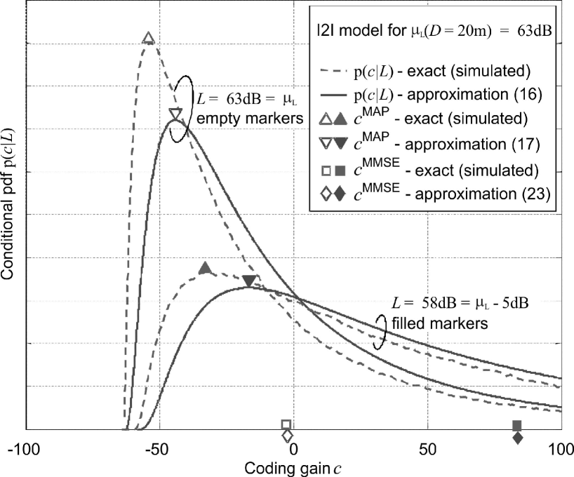
Figure 4: Conditional pdf $\mathrm{p}\left(c|L\right)$, both exact (simulated) and approximated (analytical). The respective link quality estimators $\hat{c}_{i,j}^{\mathrm{MAP}}$ and $\hat{c}_{i,j}^{\mathrm{MMSE}}$ are also depicted for two values of observed path loss $L$ (empty markers for $L=63\mathrm{dB}$ and filled markers for $L=58\mathrm{dB}$).

where $u(x)$ is the unitary step function. The approximation is corroborated by a numerical analysis in Fig. 4, where the true and the approximated pdfs are shown for two values of the path loss $L$ of one I2I link, simulated according to the model calibration in Sect. III-B.

Based on the a-posteriori pdf, we derive the maximum a posteriori (MAP) estimator of the link quality $c$. The MAP estimator, $\hat{c}^{\mathrm{MAP}}=\arg\underset{c}{\max}\left[\mathrm{p}(c|L)\right]$, is approximated by the mode value of the shifted log-normal distribution (16) which yields [25]:

$$\begin{array}[]{l}\hat{c}^{\mathrm{MAP}}\approx\Upsilon\theta\left(\mu_{\mathrm{K|L}}-\frac{\sigma_{\mathrm{K|L}}^{2}}{\Upsilon}\right)-L\end{array}.$$ (17)

A minimum mean square error (MMSE) estimator $\hat{c}^{\mathrm{MMSE}}$ is also provided in Appendix B. The MAP and MMSE estimators are depicted, by empty markers for $L=63\mathrm{dB}$, and by filled ones for $L=58\mathrm{dB}$ in Fig. 4, together with the corresponding pdfs. The figure shows that the approximations of the pdfs and of the estimators are tight to the exact ones, and behave similarly with varying path loss value.

IV Partner Selection Strategies

In this section, the problem we tackle is how to select the partner for the nodes that are tasked to communicate to the outdoor AP. The final goal is to minimize the maximum energy consumed among them. The AP selects the partners (relays) based on long-term link quality metrics and not on the instantaneous channel gains, as proposed and studied in the literature (e.g., in [7]). The optimal min-max pairing is found in Sect. IV-A that allows also for configurations with un-paired nodes. To lower the complexity and the amount of signaling, a worst-link-first (WLF) algorithm is then described in Sect. IV-B. Although the structure of the WLF algorithm is simple and resembles the one in [8] - with a modification for odd number of nodes - the proposed performance analysis diverges substantially for the I2I/I2O fixed links considered in our experimental scenario (see Sect. III). Given that the distributed wireless links can be modeled by Rician fading with different K-factors, the first key idea is that the AP uses the coding gain and not the path loss as decision metric in the WLF algorithm. Secondly, the Bayesian estimators derived in Sect. III-C provide a representation of the link quality to be used by the AP to finalize the partner selection.

IV-A Problem Definition and Optimal Solver

We define the set of candidate pairing sets $\mathcal{P}$, such that one set $\xi\in\mathcal{P}$ contains up to $\left\lfloor N/2\right\rfloor$ disjoint pairs of cooperative nodes: $\xi=\left\{(i,j),(k,h),...,(f,g)\right\}.$ All the non-paired nodes belong to the set of single nodes $\mathcal{S_{\xi}}=\left\{q,s,\ldots,z\right\}$, such that $2\left|\mathcal{\xi}\right|+\left|\mathcal{S_{\xi}}\right|=N$ (where $\left|\cdot\right|$ denotes the cardinality of the set). Given the candidate pairing set $\xi$ and the corresponding single node set $\mathcal{S_{\xi}}$, the maximum energy consumed by a node in the network is $E^{\mathrm{max}}(\xi)=\max[\max\limits_{(i,j)\in\xi}E_{(i,j),0}^{\mathrm{max}},\;\max\limits_{q\in\mathcal{S_{\xi}}}E_{q}]$, where $E_{(i,j),0}^{\mathrm{max}}=\max[E_{(i,j),0},\,E_{(j,i),0}]$ is the maximum energy for the pair $(i,j)$ for a given relaying protocol, with $E_{(i,j),0}$ defined by (11). The optimal pairing $\hat{\xi}$ is the solution to

$$\hat{\xi}=\arg\min_{\xi\in\mathcal{P}}E^{\mathrm{max}}(\xi)$$ , (18)

where we assume that all nodes have the same rate $R$ and outage probability $p$ constraints.

The problem (18) can be formulated as a special case of the weighted matching problem on the non-bipartite graph $\mathcal{G=}(\mathcal{X},\mathcal{E})$ [26]. The set of vertices $\mathcal{X}$ corresponds to the set of nodes $\left\{1,\ldots,N\right\}$, which are fully connected by the set of undirected edges $\mathcal{E}=\left\{e_{i,j}:\>\left(i,j\in\mathcal{X}\right)\>\&\>\left(i\leq j\right)\right\}$. The loops $e_{i,j=i}$ can be regarded as edges $e_{i,\bar{i}}$, where the virtual vertex $\bar{i}$ of the extended graph is connected only to $i$. The weights $w\left(e_{i,j<i}\right)=E_{(i,j),0}^{\mathrm{max}}$ and $w\left(e_{i,j=i}\right)=E_{i}$ are associated to all the edges and loops, respectively. The optimal pairing algorithm removes at each iteration the maximum weighted edge of the extended graph (as done in [27] for a max-min problem on the bipartite graph) and checks the existence of a weighed matching solution in the remaining graph using Gabow’s algorithm [26, Ch. 11], which was instead proposed in [8] for minimizing the sum of the energies consumed at the nodes in one iteration only. It can be shown that the above algorithm reaches the solution in $O\left(N^{5}\right)$ computational time. Notice that the algorithm is centralized and requires the AP to know all the inter-node link qualities for computing $c_{\left(i,j\right),0}$.

IV-B Worst-Link-First Coding-Gain Based (WLF-CG) algorithm

The WLF algorithm is a suboptimal protocol for node pairing that allows to reduce the complexity to $O\left(N^{2}\right)$. The conventional WLF algorithm (referred to as WLF path-loss-based, WLF-PL) is based on the information of second order statistics of the fading link [8], i.e. the path loss $L_{i,j}$. We propose a WLF method based on the coding gain (WLF-CG).

Link quality estimation – Before pairing decisions can take place, each node $i$ locally acquires an estimate of the link qualities for all I2I links $\hat{c}_{i,j}$ to the candidate partners and the I2O link towards the AP $\hat{c}_{i,0}$. Link quality estimator options $\hat{c}_{i,j}^{\mathrm{K}}$, $\hat{c}_{i,j}^{\mathrm{MAP}}$, and $\hat{c}_{i,j}^{\mathrm{MMSE}}$ (in dB) have been discussed in Sect. III-C. The WLF-PL algorithm uses $\hat{c}_{i,j}=-L_{i,j}$.

Protocol structure – The algorithm is composed of two phases:

1) Candidate partner set discovery – Each node $i$ performs link quality estimation $\hat{c}_{i,0}$ for the I2O channel exploiting the periodic transmission of beacon subframes from the AP as probing signals to be used for channel parameter estimation. The link qualities $\hat{c}_{i,j}$ measured from all neighboring nodes over I2I links are estimated based on the signals overheard from the potential partners. The difference $\hat{c}_{i,j}-\hat{c}_{i,0}$ is compared at each node $i$ to a common threshold $\tau$ in order to guarantee the condition $\theta(\hat{c}_{i,j})\gg\theta(\hat{c}_{i,0})$. If $\hat{c}_{i,j}-\hat{c}_{i,0}>\tau$ then node $j$ becomes a candidate partner for node $i$. Given the I2O link quality estimation $\hat{c}_{i,0}$, the threshold $\tau$ is centrally designed such that the probability of finding no candidate partners among the $N-1$ potential candidates $\prod_{j=1,j\neq i}^{N}\left[1-\Pr\left(c_{i,j}>\hat{c}_{i,0}+\tau|L_{i,j}\right)\right]$ is small enough, where $\Pr\left(c_{i,j}>\hat{c}_{i,0}+\tau|L_{i,j}\right)$ can be estimated using (16). The evaluation of the optimal value for the threshold $\tau$ is carried out in the case-study outlined in Sect. V. The candidate partners set $\mathcal{C_{P}}(i)=\{j\,:\,\hat{c}_{i,j}-\hat{c}_{i,0}>\tau\}$ is finally communicated to the AP from each node $i$, using the assigned subframe.

2) Assignment algorithm at the AP – At each iteration the AP selects the worst-uplink node $i$ with link quality $\hat{c}_{i,0}<\hat{c}_{k,0}\mbox{ }$,$\forall k\neq i$, and, if possible, assigns it to the best-uplink candidate partner $j$, such that

$$j=\arg\max_{j\in\mathcal{C_{P}}(i)}\mbox{ }\hat{c}_{j,0}$$ (19)

Nodes $i$ and $j$ are paired and disregarded in the next iterations, unless $\mathcal{C_{P}}(i)$ is empty. In the latter case, node $i$ is left un-paired in the final configuration.

For an odd number of nodes $N$ the preliminary step is to leave the best-uplink node un-paired, then the partner assignment follows as above for the remaining $N-1$ nodes.

V Experimental Assessment of Partner Selection in the I2O Environment

In what follows, we provide numerical simulations on the performance of the partner selection algorithms (Sect. IV) and of the Bayesian link quality estimation methods (Sect. III-C). The network setup is outlined in Fig. 1, $N$ nodes are randomly distributed in a $25\mathrm{m}\times 25\mathrm{m}$ indoor environment, while the AP is placed outdoors $50\mathrm{m}$ away from the nearest wall. For each random topology of the network, K-factor and path loss values are generated independently for all links according to the respective I2I and I2O models detailed in Sect. III-B. The performance results are expressed in terms of lifetime gain $\mathbb{E}[E^{\mathrm{max}}(\xi_{\mathrm{ref}})]/\mathbb{E}[E^{\mathrm{max}}(\hat{\xi})]$, defined as the ratio between the maximum energies (averaged over $5\times 10^{4}$ random topologies) consumed among the nodes according to two different pairing strategies: the reference protocol with pairing solution $\xi_{\mathrm{ref}}$ and the proposed protocol with pairing solution $\hat{\xi}$. Note that the largest values of $E^{\mathrm{max}}(\xi_{\mathrm{ref}})$ and of $E^{\mathrm{max}}(\hat{\xi})$ highlight the lifetime gain in scenarios where the I2O channel conditions are worst. In the examples, the energies consumed for reception $E_{\text{RX}}$ and for basic processing $E_{\text{p}}$ are neglected. According to the I2O modeling in Sect. III, it is likely that $c_{i,j}\gg\max\left[c_{i,0},\,c_{j,0}\right]$. From (10), the optimal choice for slot duration is $\beta_{i}=\beta_{j}=1/2$. We set $\Gamma=1$, as this assumption has no relevant impact on the performance comparisons in the examples. The target outage probability is $p=10^{-3}$ for all the nodes with spectral efficiency $R=1\,\mathrm{bps/Hz}$.

In Sect. V-A, we provide numerical simulations for the WLF-CG lifetime performance. In Sect. V-B, the impact of the proposed link quality estimation is evaluated and compared to the case where a noisy estimation of the K-factor is obtained from training. Finally, in Sect. V-C, the proposed pairing algorithm performance is discussed in presence of imperfect modeling of the channel.

V-A WLF-CG Protocol Performance

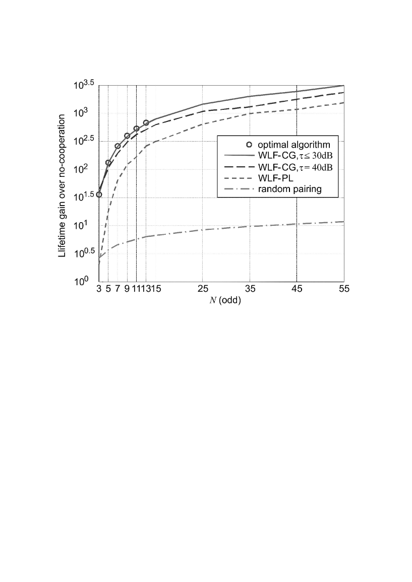
Figure 5: Cooperative transmission lifetime gain over no-cooperation with different partner selection strategies and varying number of transmitting nodes $N$ (odd values). The WLF-CG uses threshold values $\tau=\{30\mathrm{dB},40\mathrm{dB}\}$ for $\hat{c}_{i,j}-\hat{c}_{i,0}$ in the candidate partner set discovery phase. The conservative choice $\tau=-\infty$ is used for the WLF-PL.

We first evaluate the performance of the WLF-CG algorithm assuming that the link qualities $c_{i,j}$ are perfectly known at the respective nodes $i=\{1,\ldots,N\}$ and $j=\{0,\ldots,N\}$. Fig. 5 shows the lifetime gain of AF cooperation compared to no-cooperation, i.e. $\xi_{\mathrm{ref}}=\oslash$ is the empty pairing set and $\hat{\xi}$ is the pairing set obtained according to a partner selection strategy. A random pairing strategy is also considered for comparison where all nodes are disjointly paired with a random choice of the partner. For odd $N$, the optimal pairing algorithm in Sect. IV-A, the random pairing strategy, the WLF-PL algorithm, and the proposed WLF-CG are compared. The candidate partner conditions (see Sect. IV-B) $c_{i,j}\gg c_{i,0}$ and $L_{i,j}\ll L_{i,0}$ for the WLF-CG and the WLF-PL, respectively, are almost always guaranteed for each pair of nodes, in particular it is $\Pr\left(c_{i,j}>c_{i,0}+\tau\right)\simeq 1$ and $\Pr\left(L_{i,j}<L_{i,0}-\tau\right)\simeq 1$ for $\tau\leq 30\mathrm{dB}$. For the propagation environment under consideration, the simulations show that partner selection performance get worse when choosing $\tau\geq 40\mathrm{dB}$. The exploitation of the knowledge of the K-factor is revealed crucial: the WLF-CG algorithm increases the lifetime from a factor of 20 for $N=3$ to a factor of 2 for $N=55$ compared to the WLF-PL. This results from the fact that the WLF-CG algorithm allows for a more efficient exploitation of the available diversity, as if the optimal algorithm in Sect. IV-A were applied. The remarkable gains over no-cooperation and over the random pairing denote a large degree of spatial redundancy provided by the multi-link channel, i.e., the path loss and K-factor values exhibit significant variations over the space.

V-B Impact of Link Quality Estimation on WLF-CG

The optimality of the WLF-CG pairing strategy relies on the accuracy of coding gain (link quality) estimation. This motivates a closer study to identify the most suitable estimator and to quantify the benefits provided by the knowledge of the distributed channel model. Here, we assume that only the path loss $L$ is perfectly known.

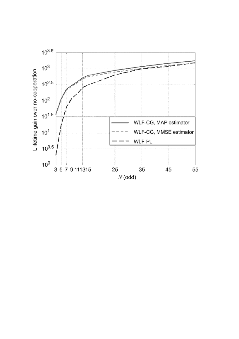
Figure 6: The lifetime gains of the WLF-CG algorithm based on $\hat{c}_{i,j}^{\mathrm{MAP}}$ and $\hat{c}_{i,j}^{\mathrm{MMSE}}$ over no-cooperation, compared to that of WLF-PL, with varying number of transmitting nodes $N$ (odd values).

Link quality estimation from the path loss $\hat{c}_{i,j}=\left\{\hat{c}_{i,j}^{\mathrm{MAP}},\hat{c}_{i,j}^{\mathrm{MMSE}}\right\}$ – The WLF-CG algorithm can capitalize from the available site-specific channel characterization. Fig. 6 shows the energy gains of cooperation over no-cooperation for varying number of cooperating nodes $N$. The estimators $\hat{c}_{i,j}^{\mathrm{MAP}}$ and $\hat{c}_{i,j}^{\mathrm{MMSE}}$ are used, exhibiting equivalent performance: notably, the lifetime gain over the WLF-PL ranges between factors 2 ($N=15$) and 20 ($N=3$). These gains are similar to those obtained in the case where $c_{i,j}$ are perfectly known (see Fig. 5). Thus, the proposed Bayesian estimation of $c$ is revealed useful to guarantee significant lifetime benefits in the considered network settings.

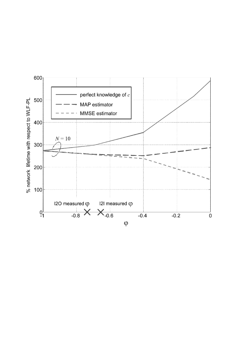
Figure 7: Lifetime performance of the WLF-CG algorithm, also with MAP and MMSE estimators, compared in percentage to the one of the WLF-PL (100% means equal performance). The correlation $\varphi$ between path loss and K-factor as defined in (12) is varying and is assumed equal for both the I2I links and the indoor component of the I2O links. As practical reference, the cross markers highlight the values $\varphi=-0.66$ and $\varphi=-0.74$, i.e., the correlation observed in the I2I and in the indoor component of the I2O measurements, respectively.

In Fig. 7 we evaluate how the WLF-CG lifetime gain scales with the correlation $\varphi$ between the path loss and the K-factor for $N=10$. The correlation $\varphi$ (assumed equal for both the I2I links and the indoor component of the I2O links) varies arbitrarily from $-1$ to $0$, whereas the other channel parameters conform to the values in Table 1. When the link quality $c$ is known, the lifetime gain increases as $\varphi$ gets closer to 0: this is the case where the knowledge of the K-factor becomes in theory most beneficial. Instead, the WLF-CG algorithm based on $\hat{c}_{i,j}^{\mathrm{MAP}}$, and $\hat{c}_{i,j}^{\mathrm{MMSE}}$ is shown not to be sensitive within realistic variations $-0.8<\varphi<-0.5$, as it improves always by a factor 2.5 the lifetime obtained by employing the WLF-PL. It is interesting to observe that $\hat{c}_{i,j}^{\mathrm{MAP}}$ performs better than $\hat{c}_{i,j}^{\mathrm{MMSE}}$ for $\varphi>-0.4$, as it is more conservative in predicting the worst-uplink link quality, which dominates the lifetime performance. Indeed, it can be verified that $\hat{c}_{i,j}^{\mathrm{MAP}}\leq\hat{c}_{i,j}^{\mathrm{MMSE}}$.

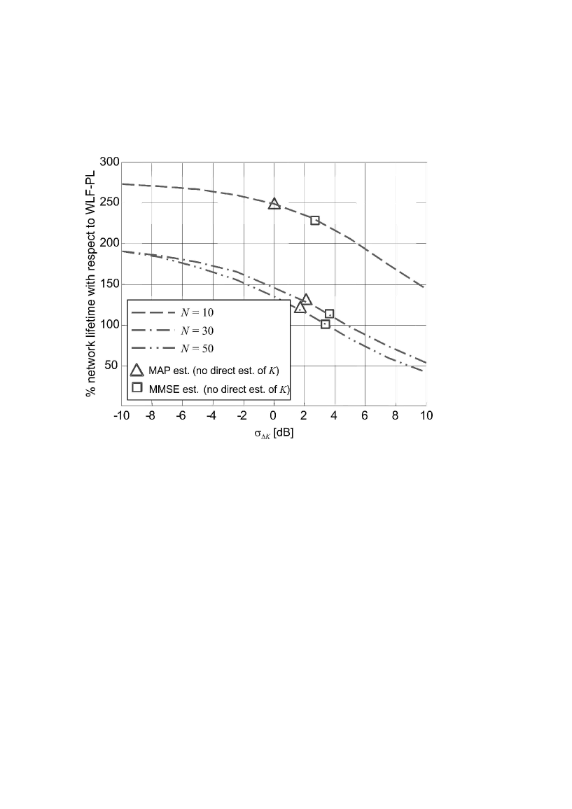
Figure 8: WLF-CG lifetime compared in percentage to WLF-PL, with varying K-factor estimation MSE. The lifetime performance of the WLF-CG algorithm based on $\hat{c}_{i,j}^{\mathrm{MAP}}$ and $\hat{c}_{i,j}^{\mathrm{MMSE}}$ are also marked on the respective curves for comparison.

Link quality estimation from both path loss and K-factor $\hat{c}_{i,j}=\hat{c}_{i,j}^{\mathrm{K}}$ – The estimator of the K-factor can be obtained from the complex fading realizations or the corresponding squared envelope values (acquired from RSSI measurements) [23]. As discussed in Sect. III-C, depending on the choice of the estimator, various trade-offs between accuracy and complexity can be obtained. Here, we prefer not to consider any specific estimator $\hat{K}$, but we rather model the estimation noise $\theta\left(\hat{K}\right)-\theta\left(K\right)$ as zero-mean Gaussian, where the pdf is truncated in order to keep $\theta\left(\hat{K}\right)$ positive. Fig. 8 shows the lifetime gain of the WLF-CG algorithm with the direct estimate $\hat{c}_{i,j}=\hat{c}_{i,j}^{\mathrm{K}}$ over the WLF-PL, with varying root mean squared error (RMSE) $\sigma_{\bigtriangleup K}=\sqrt{\mathbb{E}\left[\left|\theta\left(\hat{K}\right)-\theta\left(K\right)\right|^{2}\right]}$. Remarkably, for $N=10$ and $\sigma_{\bigtriangleup K}\leq 5\mathrm{\mathrm{d}B}$ the lifetime is at least doubled. Notice that $\hat{c}_{i,j}^{\mathrm{MAP}}$ outperforms $\hat{c}_{i,j}^{\mathrm{MMSE}}$, resulting in lifetime gains as if $\hat{c}_{i,j}^{\mathrm{K}}$ were employed with $\sigma_{\bigtriangleup K}=0\mathrm{\mathrm{d}B}$, and $3\mathrm{\mathrm{d}B}$, respectively. The estimator of $\hat{c}_{i,j}^{\mathrm{K}}$ is revealed robust for partner selection for a small number of cooperating nodes $N$. Instead, for larger number of nodes $N\geq 30$, the lifetime is doubled only for $\sigma_{\bigtriangleup K}\leq-10\mathrm{\mathrm{d}B}$, while the WLF-CG is even outperformed by the WLF-PL for $\sigma_{\bigtriangleup K}>6\mathrm{dB}$.

V-C Impact of Imperfect Model Knowledge

We consider a protocol where a set of $N_{1}$ nodes is used in a prior communication session to update the channel model, as shown in Fig. 1. In a later communication session, $N_{2}$ different nodes are then tasked to transmit to the AP. The impairment of the model knowledge is due to the limited number of the $(K,L)$ regression points used in the prior session to estimate the model, i.e., $(N_{1}^{2}-N_{1})/2$ points for the I2I model and $N_{1}$ points for the I2O model. Thus, the accuracy of the proposed Bayesian link quality estimation improves for increasing $N_{1}$, at the expense of spectral and computational power efficiency. This trade-off is assessed in the following. We focus on the MAP estimator $\hat{c}_{i,j}^{\mathrm{MAP}}$, that was shown to have better performance compared to $\hat{c}_{i,j}^{\mathrm{MMSE}}$ in the above evaluations.

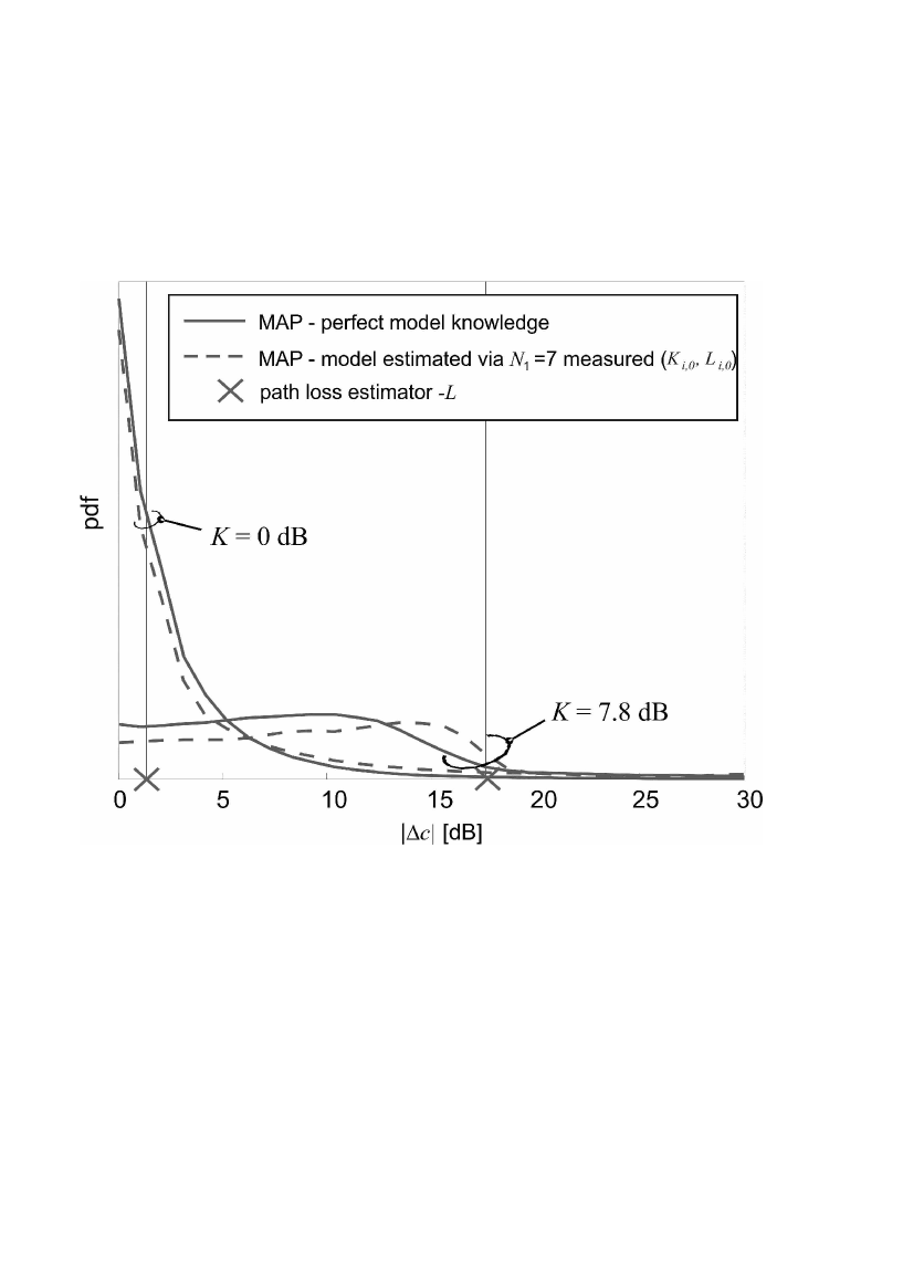
Figure 9: I2O coding gain absolute estimation error $\left|\Delta c\right|=\left|\hat{c}_{i,0}-c_{i,0}\right|$ pdf for the estimator $\hat{c}_{i,0}=\hat{c}_{i,0}^{\mathrm{MAP}}$ with perfect model knowledge (solid lines) compared to that with the model estimated via $N_{1}=7$ points ($L_{i,0}$,$K_{i,0}$) observed in the previous communication session (dashed lines). Also the estimation error $\varsigma(K)=c_{i,0}+L_{i,0}$ in the WLF-PL is depicted for the considered values of the K-factor $K_{i,0}=\{0\mathrm{dB},7.8\mathrm{dB}\}$, i.e., $\theta(K_{i,0})=\{1,6\}$.

Fig. 9 shows the pdfs of the I2O coding gain estimation absolute error in dB $\Delta_{c}=|\hat{c}_{i,0}-c_{i,0}|$ for the estimator $\hat{c}_{i,0}^{\mathrm{MAP}}$ with perfect (solid lines) and imperfect model knowledge derived via $N_{1}=7$ nodes (dashed lines) for $K_{i,0}=\{0\mathrm{dB},7.8\mathrm{dB}\}$. Notably, the absolute error pdfs are very similar, although the bivariate model is estimated by only 7 spatially distinct measurements of $(K_{i,0},L_{i,0})$. As expected, the mean points of $\Delta_{c}$ in the considered range of K-factor values, i.e., >0dB and <7.8dB, are smaller than the absolute error of the link quality estimator used in the WLF-PL, i.e., $\varsigma(K)=c_{i,0}+L_{i,0}$ (depicted by the cross markers).

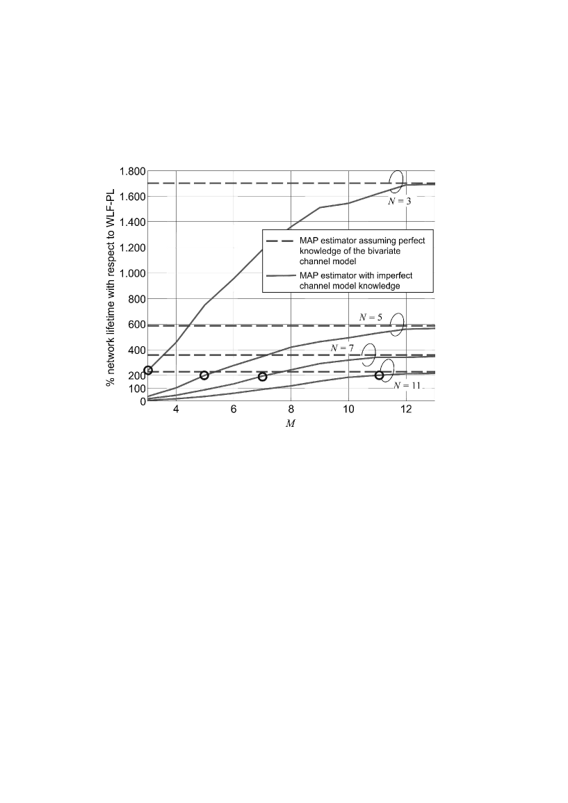
Figure 10: WLF-CG lifetime with MAP link-quality estimator $\hat{c}_{i,j}^{\mathrm{MAP}}$ compared in percentage to WLF-PL, with varying number of nodes $N_{1}$ involved in the the estimation the bivariate channel model during the previous communication session. The lifetime gains of the WLF-CG algorithm based on $\hat{c}_{i,j}^{\mathrm{MAP}}$ with perfect model knowledge are also depicted with dashed lines as upper bound. Performance for different values of communicating nodes $N_{2}$ in the current session are depicted. The circle markers highlight the performance for $N_{1}=N_{2}$.

Fig. 10 plots the network lifetime gains of the WLF-CG that uses $\hat{c}_{i,j}=\hat{c}_{i,0}^{\mathrm{MAP}}$ over the WLF-PL with varying number of the nodes $N_{1}$ employed for the parameter extraction. The performance with perfect model knowledge is also depicted as upper bound. It is revealed that, for $3<N_{2}<11$, the proposed WLF-CG algorithm outperforms the WLF-PL, by at least doubling the network lifetime for $N_{1}\geq N_{2}$ (as highlighted by circle markers).

VI Concluding Remarks

We have designed an efficient partner selection protocol for cooperative wireless access from fixed indoor nodes to an outdoor AP through AF relaying. Given that the considered links can be modeled by Rician fading, we have proposed a partner selection algorithm that adopts the coding gain - a function of the path loss and K-factor - as link quality metric for pairing the nodes. The proposed approach implies an additional computational cost due to the estimation of the K-factor, but provides a network lifetime increase by factors ranging from 2 to 20 compared to the conventional algorithm based on path loss information only.

Analyzing measurement data from a channel sounding campaign at 2.4GHz we were able to characterize the path loss and the K-factor with a Gaussian bivariate model. From this bivariate model a novel link quality indicator is derived that does not require a permanent re-estimation of the K-factors. This is the Bayesian estimate of the coding gain, where the path loss is the observed variable (inferred through RSSI readings) and the channel model is the a-priori information. The novel metric improves remarkably the partner selection performance almost as if full knowledge of the K-factors were available.

Furthermore, the analysis on the measurement data reveals the high degree of spatial coherence of the model. Hence, we have proposed a protocol with two phases: (i) for a long time period (within the stationarity time interval of the model) low-complexity communication sessions take place, where the link qualities are inferred through path loss measurements and the a-priori information of the channel model; (ii) for a short time period, a more complex communication session occurs, where a set of nodes estimate also the K-factors in order to update the site-specific channel model. Numerical results show a good trade-off between performance and robustness. In particular, the proposed protocol allows to double the network lifetime compared to the conventional algorithm, also in presence of modeling mismatches.

Appendix A

For Rician fading where $\rho_{(i,j),0}=\sqrt{\rho_{i}\rho_{j}}$ and $d_{(i,j),0}=2$, the target outage probability $p$ constrains the powers $\rho_{i}$ and $\rho_{j}$ over the two slots such that repetition based coding prescribes that $\beta_{i}=\beta$ and $1-\beta_{j}=\beta$:

$$\begin{array}[]{c}\rho_{j}\geq\frac{1}{2}\left[\frac{\sigma^{2}\left(2^{R/(1-\beta)}-1\right)}{\Gamma c_{\left(j,i\right),0}}\right]^{2}\left(p\rho_{i}\right)^{-1},\;\rho_{i}\geq\frac{1}{2}\left[\frac{\sigma^{2}\left(2^{R/\beta}-1\right)}{\Gamma c_{\left(i,j\right),0}}\right]^{2}\left(p\rho_{j}\right)^{-1}.\end{array}$$ (20)

Recall that the gap $\Gamma$ can be designed to be the same for the communication both from $i$ and from $j$. By minimizing the maximum over $\rho_{i}$ and $\rho_{j}$, the simple power balancing solution $\rho_{i}=\rho_{j}=\kappa(\hat{\mathrm{\beta}})\sigma^{2}/\sqrt{2p}$ is found where $\kappa(\beta)=\max\left[\left(2^{R/\beta}-1\right)/\left(\Gamma c_{\left(i,j\right),0}\right),\>\left(2^{R/(1-\beta)}-1\right)/\left(\Gamma c_{\left(j,i\right),0}\right)\right]$ and $\hat{\mathrm{\beta}}=\arg\underset{\beta}{\min}\kappa(\beta)$ is solution to $\left(2^{R/\hat{\beta}}-1\right)c_{\left(j,i\right),0}=\left(2^{R/\left(1-\hat{\beta}\right)}-1\right)c_{\left(i,j\right),0},$ therefore

$$2^{R/\hat{\beta}}-1=\lambda\left(2^{R/\left(1-\hat{\beta}\right)}-1\right)$$ (21)

where $\lambda=\sqrt{\frac{1+c_{i,0}/c_{i,j}}{1+c_{j,0}/c_{i,j}}}$ . The solution to (21) is now approximated for large enough rate $R$ such that for $\log_{2}(\lambda)\ll R$ it is

$$\frac{R}{\hat{\beta}}-\frac{R}{1-\hat{\beta}}\approx\log_{2}\lambda.$$ (22)

Now by letting $\hat{\beta}=\frac{1}{2}-\hat{\upsilon}$ with $\hat{\upsilon}$ small enough, the solution to (22) is $\hat{\upsilon}\approx\frac{\log_{2}(\lambda)}{8R}$.

Appendix B

The minimum mean square error (MMSE) estimator $\hat{c}^{\mathrm{MMSE}}$ can be approximated as

$$\hat{c}^{\mathrm{MMSE}} = \mathbb{E}\left[c|L\right]\approx\mathbb{E}\left[\Upsilon\theta(K)|L\right]-\mathbb{E}\left[\max\left(K,0\right)|L\right]-L=$$ (23)

$$= \Upsilon\theta\left(\mu_{\mathrm{K|L}}+\frac{\sigma_{\mathrm{K|L}}^{2}}{2\Upsilon}\right)-\mu_{\mathrm{K|L}}Q\left(-\frac{\mu_{\mathrm{K|L}}}{\sigma_{\mathrm{K|L}}}\right)-\frac{\sigma_{\mathrm{K|L}}}{\sqrt{2\pi}}\exp\left(-\frac{\mu_{\mathrm{K|L}}^{2}}{2\sigma_{\mathrm{K|L}}^{2}}\right)-L,$$

where $Q\left(\cdot\right)$ is the Q-function. In (23) we use the approximation $\varsigma(K)\simeq\Upsilon\theta(K)-\max\left(K,0\right)$ $\forall K$, where $\mathbb{E}\left[\max\left(K,0\right)|L\right]=\intop_{0}^{\infty}K\,\mbox{p}\left[K|L\right]\,\mbox{d}K$.

Table I: Parameters for the Bivariate Model (12) - see Sect. III-B

	Bivariate Model (12) Parameters
$\begin{array}[]{c}\mbox{Indoor-to-Indoor (I2I)}:\\ (i,j)\neq 0;\>D=D_{i,j}\end{array}$	$\begin{array}[]{c}\\ \mu_{\mathbf{x}}\begin{cases}\mathcal{\mu_{\mathrm{K}}}(D|_{\mathrm{m}})=16.90-10\alpha_{K}\log_{10}\left(D|_{\mathrm{m}}\right)\\ \mathcal{\mu_{\mathrm{L}}}(D|_{\mathrm{m}})=40.4+10\alpha_{\mathrm{L}}\log_{10}\left(D|_{\mathrm{m}}\right)\end{cases}\\ \\ \left[\alpha_{\mathrm{K}}=0.53,\>\alpha_{\mathrm{L}}=1.75\right]\\ \\ \mathbf{C}\begin{cases}\varphi=-0.66\\ \mbox{ }\sigma_{\mathrm{K}}=5.8\mathrm{dB},\mbox{ }\sigma_{\mathrm{L}}=6\mathrm{dB}\end{cases}\\ \\ \end{array}$
$\begin{array}[]{c}\mathrm{\mbox{Indoor-to-Outdoor (I2O),}}\\ \mbox{Outdoor propagation $K_{\mathrm{Wall}\mathrm{,0}}\mbox{ and }L_{\mathrm{Wall}\mathrm{,0}}$:}\\ (\mathrm{wall},\>j=0\mbox{ });\>D=D_{\mathrm{wall},0}\end{array}$	$\begin{array}[]{c}\\ \mu_{\mathbf{x}}\begin{cases}\mathcal{\mu_{\mathrm{K}}}(D|_{\mathrm{km}})=7.85-10\alpha_{K}\log_{10}\left(D|_{\mathrm{km}}\right)\\ \mathcal{\mu_{\mathrm{L}}}(D|_{\mathrm{km}})=135.78+10\alpha_{\mathrm{L}}\log_{10}\left(D|_{\mathrm{km}}\right)\end{cases}\\ \\ \left[\alpha_{\mathrm{K}}=0.45,\>\alpha_{\mathrm{L}}=3.89\right]\\ \\ \mathbf{C}\begin{cases}\varphi=-0.25\\ \mbox{ }\sigma_{\mathrm{K}}=7.5\mathrm{dB},\mbox{ }\sigma_{\mathrm{L}}=7.9\mathrm{dB}\end{cases}\\ \\ \end{array}$
$\begin{array}[]{c}\mathrm{\mbox{Indoor-to-Outdoor (I2O),}}\\ \mbox{Indoor propagation $K_{i,\mathrm{Wall}}\mbox{ and }L_{i,\mathrm{Wall}}$:}\\ (i\neq 0,\mbox{ }\mathrm{wall});\>D=D_{i,\mathrm{wall}}\end{array}$	$\begin{array}[]{c}\\ \mu_{\mathbf{x}}\begin{cases}\mathcal{\mu_{\mathrm{K}}}(D|_{\mathrm{m}})=-0.3D|_{\mathrm{m}}\\ \mathcal{\mu_{\mathrm{L}}}(D|_{\mathrm{m}})=0.5D|_{\mathrm{m}}\end{cases}\\ \\ \mathbf{C}\begin{cases}\varphi=-0.74\\ \sigma_{\mathrm{K}}=5.7\mathrm{dB},\mbox{ }\sigma_{\mathrm{L}}=7\mathrm{dB}\end{cases}\\ \\ \mbox{ }\end{array}$

References

- [1] C. Gomez and J. Paradells, “Wireless home automation networks: a survey of architectures and technologies,” IEEE Commun. Mag., Jun. 2010.
- [2] A. Willig, “Recent and emerging topics in wireless industrial communications: a selection,” IEEE Trans. Industr. Inf., vol. 4, pp. 102–123, May 2008.
- [3] Y. Chen and Q. Zhao, “On the lifetime of wireless sensor networks,” IEEE Commun. Letters, vol. 9, pp. 976–978, Nov. 2005.
- [4] S. Cui, A. J. Goldsmith, and A. Bahai, “Energy-efficiency of MIMO and cooperative MIMO techniques in sensor network,” IEEE J. Sel. Areas Commun., vol. 22, pp. 1089–1098, Aug. 2004.
- [5] T. E. Hunter and A. Nosratinia, “Distributed protocols for user cooperation in multi-user wireless networks,” in Proc. of IEEE GLOBECOM, pp. 3788–3792, 2004.
- [6] P. Liu, Z. Tao, Z. Lin, E. Erkip, and S. Panwar, “Cooperative wireless communications: a cross-layer approach,” IEEE Wireless Commun. Mag., vol. 13, pp. 84–92, Aug. 2006.
- [7] A. Bletsas, A. Khisti, D. P. Reed, and A. Lippman, “A simple cooperative diversity method based on network path selection,” IEEE J. Sel. Areas Commun., vol. 24, pp. 659–672, Mar. 2006.
- [8] V. Mahinthan, L. Cai, J. W. Mark, and X. Shen, “Partner selection based on optimal power allocation in cooperative-diversity systems,” IEEE Trans. Veh. Technol., vol. 57, pp. 511–520, Jan. 2008.
- [9] M. Zorzi and R. R. Rao, “Geographic random forwarding (GeRaF) for ad hoc and sensor networks: multihop performance,” IEEE Trans. Mobile Comp., vol. 2, pp. 337–348, Dec. 2003.
- [10] Z. Lin, E. Erkip, and A. Stefanov, “Cooperative regions and partner choice in coded cooperative systems,” IEEE Trans. Commun., vol. 54, pp. 1323–1334, Jul. 2006.
- [11] J. N. Laneman, D. N. C. Tse, and G. W. Wornell, “Cooperative diversity in wireless networks: efficient protocols and outage behavior,” IEEE Trans. Inf. Theory, vol. 50, pp. 3062–3080, December 2004.
- [12] E. Callaway et al., “Home networking with IEEE 802.15.4: a developing standard for low-rate wireless personal area networks,” IEEE Commun. Mag., Aug. 2002.
- [13] K. Srinivasan and P. Levis, “RSSI is under appreciated,” in Proc. of EmNets, 2006.
- [14] L. J. Greenstein et al., “Ricean K-factors in narrow-band fixed wireless channels: theory, experiments, and statistical models,” IEEE Trans. Veh. Technol., vol. 58, pp. 4000–4012, Oct. 2009.
- [15] N. Czink et al., “July 2008 radio measurement campaign,” tech. rep., Stanford, USA, 2008.
- [16] V. Erceg et al., “Channel models for fixed wireless applications,” tech. rep., IEEE 802.16 Broadband Wireless Access Working Group, 2003.
- [17] Z. Wang and G. B. Giannakis, “A simple and general parametrization quantifying performance in fading channels,” IEEE Trans. Commun., vol. 51, pp. 1389–1398, Aug. 2003.
- [18] S. Savazzi and U. Spagnolini, “Design criteria of two-hop based wireless networks with non-regenerative relays in arbitrary fading channels,” IEEE Trans. Commun., vol. 57, pp. 1463–1473, May 2009.
- [19] CC2510Fx Radio Datasheet. Texas Instruments, 2010, http://focus.ti.com/lit/ds/swrs055f/swrs055f.pdf.
- [20] P. Soma et al., “Analysis and modeling of multiple-input multiple-output (MIMO) radio channel based on outdoor measurements conducted at 2.5 GHz for fixed BWA applications,” in Proc. of IEEE ICC, vol. 1, pp. 272–276, 2002.
- [21] P. Kyösti et al., “WINNER II channel models,” European Commission, Sep. 2007.
- [22] CC2420 Radio Datasheet. Texas Instruments, 2007, http://focus.ti.com/lit/ds/swrs041b/swrs041b.pdf.
- [23] C. Tepedelenlioglu, A. Abdi, and G. B. Giannakis, “The Ricean K-factor: estimation and performance analysis,” IEEE Trans. Wireless Commun., vol. 2, pp. 799–810, Jul. 2003.
- [24] C. G. Koay and P. J. Basser, “Analytically exact correction scheme for signal extraction from noisy magnitude MR signals,” J. Magn. Reson., vol. 179, no. 2, pp. 317–322, 2006.
- [25] C. Walck, Handbook on statistical distributions for experimentalists. Sweden: Univ. of Stockholm Press, 2000.
- [26] C. H. Papadimitriou and K. Steiglitz, Combinatorial optimization: algorithms and complexity. USA: Dover, 1998.
- [27] Y. Chen, P. Cheng, P. Qiu, and Z. Zhang, “Optimal partner selection strategies in wireless cooperative networks with fixed and variable transmit power,” in Proc. of WCNC, pp. 4083–4087, Mar. 2007.