A class of optimal tests for symmetry based on local Edgeworth approximations

Abstract

The objective of this paper is to provide, for the problem of univariate symmetry (with respect to specified or unspecified location), a concept of optimality, and to construct tests achieving such optimality. This requires embedding symmetry into adequate families of asymmetric (local) alternatives. We construct such families by considering non-Gaussian generalizations of classical first-order Edgeworth expansions indexed by a measure of skewness such that (i) location, scale and skewness play well-separated roles (diagonality of the corresponding information matrices) and (ii) the classical tests based on the Pearson–Fisher coefficient of skewness are optimal in the vicinity of Gaussian densities.

, and

1 Introduction

1.1 Testing for symmetry

Symmetry is one of the most important and fundamental structural assumptions in statistics, playing a major role, for instance, in the identifiability of location or intercept under nonparametric conditions: see [14, 2, 15]. This importance explains the huge variety of existing testing procedures of the null hypothesis of symmetry in an i.i.d. sample $X_{1},\ldots,X_{n}$; see [8] for a survey.

Traditional tests of the null hypothesis of symmetry – the hypothesis under which $X_{1}-\theta\stackrel{{\scriptstyle d}}{{=}}-(X_{1}-\theta)$ for some location $\theta\in\mathbb{R}$, with $\stackrel{{\scriptstyle d}}{{=}}$ standing for equality in distribution – are based on standardized empirical third-order moments. Let $m^{(n)}_{k}(\theta):=n^{-1}\sum_{i=1}^{n}(X_{i}-\theta)^{k}$ and $m^{(n)}_{k}:=m^{(n)}_{k}(\bar{X}^{(n)})$, where $\bar{X}^{(n)}:=n^{-1}\sum_{i=1}^{n}X_{i}$. When the location $\theta$ is specified, the test statistic is

$$S^{(n)}_{1}(\theta):=n^{1/2}m^{(n)}_{3}(\theta)/\bigl{(}m^{(n)}_{6}(\theta)\bigr{)}^{1/2},$$ (1)

the null distribution of which, under finite sixth-order moments, is asymptotically standard normal. When $\theta$ is unspecified, the classical test is based on the empirical coefficient of skewness

$$b_{1}^{(n)}:=m_{3}^{(n)}/s^{3}_{n},$$ (2)

where $s_{n}:=(m_{2}^{(n)})^{1/2}$ stands for the empirical standard error in a sample of size $n$. More precisely, this test relies on the asymptotic standard normal distribution (still under finite moments of order six) of

$$S^{(n)}_{2}:=n^{1/2}m_{3}^{(n)}\big{/}\bigl{(}m^{(n)}_{6}-6s_{n}^{2}m^{(n)}_{4}+9s_{n}^{6}\bigr{)}^{1/2},$$ (3)

which, under Gaussian densities, asymptotically reduces to $\sqrt{n/6}b^{(n)}_{1}$.

These two tests are generally considered as Gaussian procedures, although they do not require any Gaussian assumptions and despite the fact that none of them can be considered optimal in any Gaussian sense, since asymmetric alternatives clearly cannot belong to a Gaussian universe. Despite the long history of the problem, the optimality features of those classical procedures thus are all but clear, and optimality issues, in that fundamental problem, remain essentially unexplored.

The main objective of this paper is to provide this classical testing problem with a concept of optimality that confirms practitioners’ intuition (i.e., justifying the $b^{(n)}_{1}$-based Gaussian practice), and to construct tests achieving such optimality. This requires embedding the null hypothesis of symmetry into adequate families of asymmetric alternatives. We therefore define local (in the LeCam sense) alternatives indexed by location, scale and a measure of skewness in such a way that:

1. [(ii)]

2. Location, scale, and skewness play well-separated roles (diagonality of the corresponding information matrices).

3. The traditional tests based on $b_{1}^{(n)}$ (more precisely, based on $S^{(n)}_{2}$ given in (3)) become locally and asymptotically optimal in the vicinity of Gaussian densities.

As we shall see, part (ii) of this objective is achieved by considering local first-order Edgeworth approximations of the form

$$\phi(x-\theta)+n^{-1/2}\xi(x-\theta)\phi(x-\theta)\bigl{(}(x-\theta)^{2}-\kappa\bigr{)},$$ (4)

where $\phi$ as usual stands for the standard normal density, $\kappa$ ($=3$) is the Gaussian kurtosis coefficient, $\theta$ is a location parameter, and $\xi$ a measure of skewness. Adequate modifications of (4), playing similar roles in the vicinity of non-Gaussian standardized symmetric reference densities $f_{1}$, are proposed in (2.1).

The resulting tests of symmetry (for specified as well as for unspecified location $\theta$) are valid under a broad class of symmetric densities, and parametrically efficient at the reference (standardized) density $f_{1}$. Of particular interest are the pseudo-Gaussian tests (associated with a Gaussian reference density; see Proposition 3.6), which require finite moments of order six and appear to be asymptotically equivalent (under their specified-$\theta$ version as well as under the unspecified-$\theta$ one) to the test (3) based on $b^{(n)}_{1}$, and the Laplace tests (associated with a double-exponential reference density; see Proposition 3.6), which only require moments of order four and are closely related with the tests against Fechner asymmetry derived in [3].

These tests are of a parametric nature. Since the null hypothesis of symmetry enjoys a rich group invariance structure, classical maximal invariance arguments naturally bring signs and signed ranks into the picture. Such a nonparametric approach is adopted in a companion paper [4], where we construct signed-rank versions of the parametrically efficient tests proposed here. These signed-rank tests are distribution-free (asymptotically so in case of an unspecified location $\theta$) under the null hypothesis of symmetry, and therefore remain valid under much milder distributional assumptions (for the specified location case, they are valid in the absence of any distributional assumption).

The main technical tool throughout the paper is LeCam’s asymptotic theory of statistical experiments and the properties of locally asymptotically normal (LAN) families. LAN has become a standard tool in asymptotics: see [12] or Chapters 6–9 of [17] for details. Log-likelihoods in a LAN family with $k$-dimensional parameter $\bolds{\vartheta}$ admit local quadratic approximations of the form $\bolds{\tau}^{\prime}\bolds{\Delta}^{(n)}_{\bolds{\vartheta}}-\frac{1}{2}\bolds{\tau}^{\prime}\bolds{\Gamma}_{\bolds{\vartheta}}\bolds{\tau}$, where the random vector $\bolds{\Delta}^{(n)}_{\bolds{\vartheta}}$, called a central sequence, is asymptotically normal $\mathcal{N}(\bolds{\Gamma}_{\bolds{\vartheta}}\bolds{\tau},\bolds{\Gamma}_{\bolds{\vartheta}})$ under sequences of parameter values of the form $\bolds{\vartheta}+n^{-1/2}\bolds{\tau}$ (local alternatives). Let $\phi^{*}(\bolds{\Delta})$ be an optimal test (uniformly most powerful, maximin, most stringent, …) in the Gaussian shift model describing a hypothetical observation $\bolds{\Delta}$ with distribution in the family $\{\mathcal{N}(\bolds{\Gamma}_{\bolds{\vartheta}}\bolds{\tau},\bolds{\Gamma}_{\bolds{\vartheta}})\mid\bolds{\tau}\in\mathbb{R}^{k}\}$ ($\bolds{\Gamma}_{\bolds{\vartheta}}$ specified). Those families are extremely simple, and optimal tests in that context are well known (see, e.g., Section 11.9 of [11]). Then, the sequence $\phi^{*}(\bolds{\Delta}^{(n)}_{\bolds{\vartheta}})$ is a sequence of locally asymptotically optimal (locally asymptotically uniformly most powerful, maximin, most stringent, …) tests for the original problem – where optimality is based on the local convergence of risk functions to the risk functions of Gaussian shift experiments. More analytical characterizations can be found, for instance, in [5].

1.2 Outline of the paper

The problem we are considering throughout is that of testing the null hypothesis of symmetry. In the notation of Section 1.1, $\xi$ (see (2.1) for a more precise definition) is thus the parameter of interest; the location $\theta$ and the standardized null symmetric density $f_{1}$ either are specified or play the role of nuisance parameters, whereas the scale $\sigma$ (not necessarily a standard error) always is a nuisance.

The paper is organized as follows. In Section 2.1 we describe the Edgeworth-type families of local alternatives, extending (4), that we are considering. Section 2.2 establishes the local and asymptotic normality (with respect to location, scale and the asymmetry parameters) result to be used throughout; actually, we establish a slightly stronger version of LAN, called ULAN (uniform LAN), which allows us to handle the problems related with estimated nuisance parameters. The classical LeCam theory then is used in Section 3.1 for developing asymptotically optimal procedures for testing symmetry ($\xi=0$), with specified or unspecified location $\theta$ but specified standardized symmetric density $f_{1}$. The more realistic case of an unspecified $f_{1}$ is treated in Section 3.2, where we obtain versions of the optimal (at given $f_{1}$) tests that remain valid under $g_{1}\neq f_{1}$, for specified (Section 3.2.1) and unspecified (Section 3.2.2) location $\theta$, respectively. The particular case of pseudo-Gaussian procedures (which are optimal for Gaussian $f_{1}$ but valid under any symmetric density with finite moments of order six) is studied in detail in Section 3.3 and their relation with classical tests of symmetry is discussed. We also show that the Laplace tests (which are optimal for double-exponential $f_{1}$ but valid under any symmetric density with finite fourth-order moment) are closely related to the Fechner-type tests derived in [3]. The finite-sample performances of these tests are investigated via simulations in Section 4, where they are applied to the classical skew-normal and skew-$t$ densities.

2 A class of locally asymptotically normal families of asymmetric distributions

2.1 Families of asymmetric densities based on Edgeworth approximations

Denote by $\mathbf{X}^{(n)}:=(X_{1}^{(n)},\ldots,X_{n}^{(n)}),\ n\in\mathbb{N}$ an i.i.d. $n$-tuple of observations with common density $f$. The null hypotheses we are interested in are:

1. [(a)]

2. The hypothesis $\mathcal{H}^{(n)}_{\theta}$ of symmetry with respect to specified location $\theta\in\mathbb{R}$: under $\mathcal{H}^{(n)}_{\theta}$, the $X_{i}$’s have density function

   $$x\mapsto f(x):={\sigma}^{-1}f_{1}\bigl{(}({x-\theta})/{\sigma}\bigr{)}\vspace*{-3pt}$$ (5)

   (all densities are over the real line, with respect to the Lebesgue measure) for some unspecified $\sigma\in\mathbb{R}^{+}_{0}$, where $f_{1}$ belongs to the class of standardized symmetric densities

   $$\mathcal{F}_{0}:=\biggl{\{}h_{1}\mathchoice{\nobreak\,\colon}{\nobreak\,\colon}{\nobreak\,\colon\;}{\nobreak\,\colon\;}h_{1}(-z)=h_{1}(z)\mbox{ for all $z\in\mathbb{R}$ and }\int_{-\infty}^{1}h_{1}(z)\,\mathrm{d}z=0.75\biggr{\}}.\vspace*{-3pt}$$

   The scale parameter $\sigma$ (associated with the symmetric density $f$) that we are considering here thus is not the standard deviation, but the median of the absolute deviations $|X_{i}-\theta|$; this avoids making any moment assumptions.

3. The hypothesis $\mathcal{H}^{(n)}:=\bigcup_{\theta\in\mathbb{R}}\mathcal{H}^{(n)}_{\theta}$ of symmetry with respect to unspecified location (and scale): there exist $(\theta,\sigma)$ such that the $X_{i}$’s have density (5).

In both cases, the standardized density $f_{1}$ may be specified (Section 3.1) or not (Sections 3.2–3.4). The specified-$f_{1}$ problem, however, mainly serves as a preparation for the more realistic unspecified-$f_{1}$ one.

As explained in the introduction, a characterization of efficient testing requires the definition of families of asymmetric alternatives exhibiting some adequate structure, such as local asymptotic normality, at the null. For a selected class of densities $f$ enjoying the required regularity assumptions, we therefore are embedding the null hypothesis of symmetry into families of distributions indexed by $\theta\in\mathbb{R}$ (location), $\sigma\in\mathbb{R}^{+}_{0}$ (scale) and a parameter $\xi\in\mathbb{R}$ characterizing asymmetry. More precisely, consider the class $\mathcal{F}_{1}$ of densities $f_{1}$ satisfying:

1. [(iii)]

2. (symmetry and standardization) $f_{1}\in\mathcal{F}_{0}$;

3. (absolute continuity) there exists $\dot{f}_{1}$ such that, for all $z_{1}<z_{2}$,

   $$f_{1}(z_{2})-f_{1}(z_{1})=\int_{z_{1}}^{z_{2}}\dot{f}_{1}(z)\,\mathrm{d}z;\vspace*{-3pt}$$

4. (strong unimodality) $z\mapsto\phi_{f_{1}}(z):={-\dot{f}_{1}(z)}/{f_{1}(z)}$ is monotone increasing;

5. (finite Fisher information) $\mathcal{K}(f_{1}):=\int_{-\infty}^{+\infty}z^{4}\phi^{2}_{f_{1}}(z)f_{1}(z)\,\mathrm{d}z$, hence also, under strong unimodality,

   $$\mathcal{I}(f_{1}):=\int_{-\infty}^{+\infty}\phi^{2}_{f_{1}}(z)f_{1}(z)\,\mathrm{d}z\quad\mbox{and}\quad\mathcal{J}(f_{1}):=\int_{-\infty}^{+\infty}z^{2}\phi^{2}_{f_{1}}(z)f_{1}(z)\,\mathrm{d}z\vspace*{-3pt}$$

   are finite;

6. (polynomial tails)

   $$\int_{y}^{\infty}f_{1}(z)\,\mathrm{d}z=\mathrm{O}(y^{-\beta})\qquad\mbox{as }y\to\infty\vspace*{-3pt}$$

   for some $\beta>0$ and

   $$\phi_{f_{1}}(z)=\mathrm{o}(z^{\beta/2-2})\qquad\mbox{as }z\rightarrow\infty.\vspace*{-3pt}$$

That class $\mathcal{F}_{1}$ thus consists of all symmetric standardized densities $f_{1}$ that are absolutely continuous, strongly unimodal (that is, log-concave) and have finite information $\mathcal{I}(f_{1})$ and $\mathcal{J}(f_{1})$ for location and scale, and, as we shall see, $\mathcal{K}(f_{1})$ for asymmetry, with tails satisfying (v).

For all $f_{1}\in\mathcal{F}_{1}$, denote by $\kappa(f_{1}):=\mathcal{J}(f_{1})/\mathcal{I}(f_{1})$ the ratio of information for scale and information for location; $\kappa(f_{1})$, as we shall see, for Gaussian density ($f_{1}=\phi_{1}$) reduces to kurtosis ($\kappa(\phi_{1})=3$), and can be interpreted as a generalized kurtosis coefficient. Finally, write ${\mathrm{P}}^{(n)}_{\theta,\sigma,\xi;f_{1}}$ for the probability distribution of $\mathbf{X}^{(n)}$ when the $X_{i}$’s are i.i.d. with density

$$f(x) = \sigma^{-1}f_{1}\biggl{(}\frac{x-\theta}{\sigma}\biggr{)}-\xi\sigma^{-1}{\dot{f}}_{1}\biggl{(}\frac{x-\theta}{\sigma}\biggr{)}\biggl{(}\biggl{(}\frac{x-\theta}{\sigma}\biggr{)}^{2}-\kappa(f_{1})\biggr{)}I[|x-\theta|\leq\sigma|z^{*}|]$$

$$-\operatorname{sign}(\xi)\sigma^{-1}f_{1}\biggl{(}\frac{x-\theta}{\sigma}\biggr{)}\{I[x-\theta>\operatorname{sign}(-\xi)\sigma|z^{*}|]-I[x-\theta<\operatorname{sign}(\xi)\sigma|z^{*}|]\}.\hskip 25.0pt\vspace*{-3pt}$$

Here $\theta\in\mathbb{R}$ and $\sigma\in\mathbb{R}^{+}$ clearly are location and scale parameters, $\xi\in\mathbb{R}$ is a measure of skewness, $\kappa(f_{1})$ (strictly positive for $f_{1}\in\mathcal{F}_{1}$) the generalized kurtosis coefficient just defined and $z^{*}$ the unique (for $\xi$ small enough; unicity follows from the monotonicity of $\phi_{f_{1}}$) solution of $f_{1}(z^{*})=\xi\dot{f}_{1}(z^{*})((z^{*})^{2}-\kappa(f_{1}))$. The function $f$ defined in (2.1) is indeed a probability density (non-negative, integrating up to one), since it is obtained by adding and subtracting the same probability mass

$$\frac{|\xi|}{\sigma}\int_{\theta}^{\infty}\min\biggl{(}{\dot{f}}_{1}\biggl{(}\frac{x-\theta}{\sigma}\biggr{)}\biggl{(}\biggl{(}\frac{x-\theta}{\sigma}\biggr{)}^{2}-\kappa(f_{1})\biggr{)},f_{1}\biggl{(}\frac{x-\theta}{\sigma}\biggr{)}\biggr{)}\,\mathrm{d}x$$

on both sides of $\theta$ (according to the sign of $\xi$). Note that $\xi>0$ implies $f(x)=0$ for $x-\theta<-\sigma|z^{*}|$ and $f(x)={2}{\sigma}^{-1}f_{1}((x-\theta)/\sigma)$ for $x-\theta>\sigma|z^{*}|$. Moreover, $x\mapsto f(x)$ is continuous whenever $\dot{f}_{1}(x)$ is; vanishes for $x\leq\theta+\sigma z^{*}$ if $\xi>0$, for $x\geq\theta+\sigma z^{*}$ if $\xi<0$; and is left- or right-skewed according as $\xi<0$ or $\xi>0$. As for $z^{*}$, it tends to $-\infty$ as $\xi\downarrow 0$, to $\infty$ as $\xi\uparrow 0$; in the Gaussian case, it is easy to check that $|z^{*}|=\mathrm{O}(|\xi|^{-1/3})$ as $\xi\rightarrow 0$.

The intuition behind this class of alternatives is that, in the Gaussian case, (2.1), with $\xi=n^{-1/2}\tau$ yields (for $x\in[\theta\pm\sigma z^{*}]$) the first-order Edgeworth development of the density of the standardized mean of an i.i.d. $n$-tuple of variables with third-order moment $6\tau\sigma^{3}$ (where standardization is based on the median $\sigma$ of absolute deviations from $\theta$). For a “small” value of the asymmetry parameter $\xi$, of the form $n^{-1/2}\tau$, (2.1) thus describes the type of deviation from symmetry that corresponds to the classical central limit context. Hence, if a Gaussian density is justified as resulting from the additive combination of a large number of small independent symmetric shocks, the locally asymmetric $f$ results from the same additive combination of independent but slightly skew shocks. As we shall see, the locally optimal test in such a case happens to be the traditional test based on $b_{1}^{(n)}$ (see (2)).

Besides the Gaussian one (with standardized density $\phi_{1}(z):=\sqrt{{a}/{2\uppi}}\exp(-az^{2}/2)$), interesting special cases of (2.1) are obtained in the vicinity of:

1. [(iii)]

2. The double-exponential or Laplace distributions, with standardized density

   $$f_{1}(z)=f_{\mathcal{L}}(z):=({1}/{2d})\exp(-{|z|}/{d}),\vspace*{-3pt}$$

   $\mathcal{I}(f_{1})={1}/{d^{2}}$, $\mathcal{J}(f_{1})=2$ and $\mathcal{K}(f_{1})=24d^{2}$.

3. The logistic distributions, with standardized density

   $$f_{1}(z)=f_{\mathrm{Log}}(z):=\sqrt{b}\exp\bigl{(}-\sqrt{b}z\bigr{)}/\bigl{(}1+\exp\bigl{(}-\sqrt{b}z\bigr{)}\bigr{)}^{2},\vspace*{-3pt}$$

   $\mathcal{I}(f_{1})={b}/{3}$, $\mathcal{J}(f_{1})={(12+\uppi^{2})}/{9}$ and $\mathcal{K}(f_{1})={\uppi^{2}}(120+7\uppi^{2})/45b$.

4. The power-exponential distributions, with standardized densities

   $$f_{1}(z)=f_{\exp_{\eta}}(z):=C_{\exp_{\eta}}\exp(-(g_{\eta}z)^{2\eta}),\vspace*{-3pt}$$

   $\eta\in\mathbb{N}_{0}$, $\mathcal{I}(f_{1})=2g_{\eta}^{2}\eta\Gamma(2-1/2\eta)/\Gamma(1+1/2\eta)$, $\mathcal{J}(f_{1})=1+2\eta$ and $\mathcal{K}(f_{1})={2g_{\eta}\eta}/\break{\Gamma(1+1/2\eta)}$ (the positive constants $C_{\exp_{\eta}}$, $a$, $b$, $d$ and $g_{\eta}$ are such that $f_{1}\in\mathcal{F}_{1}$).

Although not strongly unimodal, the Student distributions with $\nu>2$ degrees of freedom also can be considered here (strong unimodality indeed is essentially used as a sufficient condition for the existence of $z^{*}$ in (2.1) – an existence that can be checked directly in the Student case). Standardized Student densities take the form

$$f_{1}(z)=f_{t_{\nu}}(z):=C_{t_{\nu}}(1+a_{\nu}z^{2}/\nu)^{-(\nu+1)/2},\vspace*{-3pt}$$

with $\mathcal{I}(f_{1})=a_{\nu}{(\nu+1)}/{(\nu+3)}$, $\mathcal{J}(f_{1})=3{(\nu+1)}/{(\nu+3)}$ and $\mathcal{K}(f_{1})={15}\nu(\nu+1)/a_{\nu}(\nu-2)(\nu+3)$ ($C_{t_{\nu}}$ and $a_{\nu}$ are normalizing constants). Note that the corresponding Gaussian values, namely $\mathcal{I}(\phi_{1})=a\approx 0.4549$, $\mathcal{J}(\phi_{1})=3$ and $\mathcal{K}(\phi_{1})={15}/{a}$, are obtained by taking limits as $\nu\rightarrow\infty$.

Figures 1 and 2 provide graphical representations of some densities in the Gaussian ($f_{1}=\phi_{1}$) and double-exponential ($f_{1}=f_{\mathcal{L}}$) Edgeworth families (2.1), respectively. In the Gaussian case, the skewed densities are continuous, while the double-exponential ones, due to the discontinuity of $\dot{f}_{\mathcal{L}}(x)$ at $x=0$, exhibit a discontinuity at the origin.

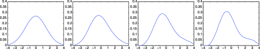
Figure 1: Graphical representation of the Gaussian Edgeworth family (2.1) ($f_{1}=\phi_{1}$), for $\xi=0$, $0.05$, $0.10$ and $0.15$.

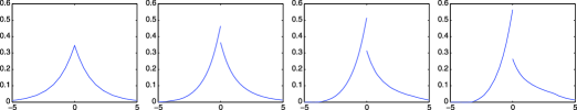
Figure 2: Graphical representation of the double-exponential Edgeworth family (2.1) ($f_{1}=f_{\mathcal{L}}$), for $\xi=0$, $0.05$, $0.10$ and $0.15$.

2.2 Uniform local asymptotic normality (ULAN)

The main technical tool in our derivation of optimal tests is the uniform local asymptotic normality (ULAN), with respect to $\bolds{\vartheta}:=(\theta,\sigma,\xi)^{\prime}$, at $(\theta,\sigma,0)^{\prime}$, of the parametric families

$$\mathcal{P}_{f_{1}}^{(n)}:=\bigcup_{\sigma>0}\mathcal{P}_{\sigma;f_{1}}^{(n)}:=\bigcup_{\sigma>0}\bigl{\{}{\mathrm{P}}_{\theta,\sigma,\xi;f_{1}}^{(n)}\mid\theta\in\mathbb{R},\xi\in\mathbb{R}\bigr{\}},\vspace*{-5pt}$$ (7)

where $f_{1}\in\mathcal{F}_{1}$. More precisely, the following result holds (see the Appendix for proof).

Proposition 2.1 ((ULAN))

For any $f_{1}\in\mathcal{F}_{1}$, $\theta\in\mathbb{R}$, and $\sigma\in\mathbb{R}^{+}_{0}$, the family $\mathcal{P}_{f_{1}}^{(n)}$ is ULAN at $(\theta,\sigma,0)^{\prime}$, with (writing $Z_{i}$ for $Z_{i}^{(n)}(\theta,\sigma):=\sigma^{-1}(X_{i}^{(n)}-\theta)$ and $\phi_{f_{1}}$ for $-\dot{f_{1}}/f_{1}$) central sequence

$$\bolds{\Delta}_{f_{1}}^{(n)}(\bolds{\vartheta}) =: \pmatrix{{\Delta}_{f_{1};1}^{(n)}(\bolds{\vartheta})\cr{\Delta}_{f_{1};2}^{(n)}(\bolds{\vartheta})\cr{\Delta}_{f_{1};3}^{(n)}(\bolds{\vartheta})}$$

$$=\hskip 3.0pt n^{-1/2}\sum_{i=1}^{n}\pmatrix{\sigma^{-1}\phi_{f_{1}}(Z_{i})\cr\sigma^{-1}\bigl{(}\phi_{f_{1}}(Z_{i})Z_{i}-1\bigr{)}\cr\phi_{f_{1}}(Z_{i})\bigl{(}Z_{i}^{2}-\kappa(f_{1})\bigr{)}}\vspace*{-3pt}$$

and full-rank information matrix

$$\bolds{\Gamma}_{f_{1}}(\bolds{\vartheta})=\pmatrix{\sigma^{-2}\mathcal{I}(f_{1})&0&0\cr 0&\sigma^{-2}\bigl{(}\mathcal{J}(f_{1})-1\bigr{)}&0\cr 0&0&\gamma(f_{1})},$$ (9)

where $\gamma(f_{1}):=\mathcal{K}(f_{1})-{\mathcal{J}^{2}(f_{1})}/{\mathcal{I}(f_{1})}$.

More precisely, for any $\bolds{\vartheta}^{(n)}:=(\theta^{(n)},\sigma^{(n)},0)^{\prime}$ such that $\theta^{(n)}-\theta=\mathrm{O}(n^{-1/2})$ and $\sigma^{(n)}-\sigma=\mathrm{O}(n^{-1/2})$, and for any bounded sequence $\bolds{\tau}^{(n)}=(t^{(n)},s^{(n)},\tau^{(n)})^{\prime}\in\mathbb{R}^{3}$, we have, under ${\mathrm{P}}_{\bolds{\vartheta}^{(n)};f_{1}}^{(n)}$, as $n\rightarrow\infty$,

$$\Lambda_{\bolds{\vartheta}^{(n)}+n^{-1/2}\bolds{\tau}^{(n)}/\bolds{\vartheta}^{(n)};f_{1}}^{(n)} := \log\biggl{(}\frac{\mathrm{d}{\mathrm{P}}_{\bolds{\vartheta}^{(n)}+n^{-1/2}\bolds{\tau}^{(n)};f_{1}}^{(n)}}{\mathrm{d}{\mathrm{P}}_{\bolds{\vartheta}^{(n)};f_{1}}^{(n)}}\biggr{)}$$

$$= \bolds{\tau}^{(n)\prime}\bolds{\Delta}_{f_{1}}^{(n)}\bigl{(}\bolds{\vartheta}^{(n)}\bigr{)}-\frac{1}{2}\bolds{\tau}^{(n)\prime}\bolds{\Gamma}_{f_{1}}(\bolds{\vartheta})\bolds{\tau}^{(n)}+\mathrm{o}_{\mathrm{P}}(1)$$

and

$${\bolds{\Delta}_{f_{1}}^{(n)}\bigl{(}\bolds{\vartheta}^{(n)}\bigr{)}\stackrel{{\scriptstyle\mathcal{L}}}{{\longrightarrow}}\mathcal{N}(\bolds{0},\bolds{\Gamma}_{f_{1}}(\bolds{\vartheta}))}.$$

The diagonal form of the information matrix $\bolds{\Gamma}_{f_{1}}(\bolds{\vartheta})$ confirms that location, scale and skewness, in the parametric family (7), play distinct and well-separated roles. The practical consequences of that orthogonality (in the sense of information) property, as we shall see, are twofold:

1. [(b)]

2. The fact that location and scale are unspecified has no cost in terms of efficiency and under specified standardized density $f_{1}$ when testing for symmetry.

3. Substituting root-$n$-consistent (and, in principle, duly discretized: see assumption (C2) below) estimators for the true values has no impact on the asymptotic validity and local powers, under specified standardized density $f_{1}$, of tests for symmetry.

Note that orthogonality between the scale and skewness components of $\bolds{\Delta}_{f_{1}}^{(n)}(\bolds{\vartheta})$ automatically follows from the symmetry of $f_{1}$, while for location and skewness, this orthogonality is a consequence of the definition of $\kappa(f_{1})$. The Gaussian versions of (2.1) and (9) are

$$\bolds{\Delta}_{\phi_{1}}^{(n)}(\bolds{\vartheta})=n^{-1/2}\sum_{i=1}^{n}\pmatrix{a\sigma^{-1}Z_{i}\cr\sigma^{-1}(aZ_{i}^{2}-1)\cr\displaystyle aZ_{i}\biggl{(}Z_{i}^{2}-\frac{3}{a}\biggr{)}}$$

and

$$\bolds{\Gamma}_{\phi_{1}}(\bolds{\vartheta})=\pmatrix{a\sigma^{-2}&0&0\cr 0&2\sigma^{-2}&0\cr 0&0&6/a},$$

respectively (recall that $a\approx 0.4549$).

3 Locally asymptotically optimal tests

The various test statistics described in this section are listed, for easy reference, in Table 5, placed at the end of Section 5.

3.1 Locally asymptotically optimal tests: Specified density

For specified $f_{1}\in\mathcal{F}_{1}$, consider the null hypothesis

$$\mathcal{H}^{(n)}_{\theta;f_{1}}:=\bigcup_{\sigma\in\mathbb{R}^{+}_{0}}\bigl{\{}{\mathrm{P}}^{(n)}_{\theta,\sigma,0;f_{1}}\bigr{\}}$$

of symmetry with respect to some specified location $\theta$, and the null hypothesis

$$\mathcal{H}^{(n)}_{f_{1}}:=\bigcup_{\theta\in\mathbb{R}}\bigcup_{\sigma\in\mathbb{R}^{+}_{0}}\bigl{\{}{\mathrm{P}}^{(n)}_{\theta,\sigma,0;f_{1}}\bigr{\}}$$

of symmetry with respect to unspecified $\theta$. ULAN and the diagonal structure of (9) imply that substituting discretized root-$n$-consistent estimators $\hat{\theta}$ and $\hat{\sigma}$ for the unknown $\theta$ and $\sigma$ has no influence, asymptotically, on the $\xi$-part of the central sequence.

Recall that a sequence of estimators $\hat{\lambda}^{(n)}$ defined in a sequence of experiments $\{{\mathrm{P}}^{(n)}_{\lambda}\mid\lambda\in\Lambda\}$ indexed by some parameter $\lambda$ is root-$n$-consistent and asymptotically discrete if, under ${\mathrm{P}}^{(n)}_{\lambda}$, as $n\rightarrow\infty$:

1. [(C2)]

2. $\hat{\lambda}^{(n)}-\lambda=\mathrm{O}_{\mathrm{P}}(n^{-1/2})$.

3. The number of possible values of $\hat{\lambda}^{(n)}$ in balls with $\mathrm{O}(n^{-1/2})$ radius centered at $\lambda$ is bounded as $n\rightarrow\infty$.

An estimator $\lambda^{(n)}$ satisfying (C1) but not (C2) is easily discretized by letting, for some arbitrary constant $c>0$, $\lambda^{(n)}_{\#}:=(cn^{1/2})^{-1}\operatorname{sign}(\lambda^{(n)})\lceil cn^{1/2}|\lambda^{(n)}|\rceil$, which satisfies both (C1) and (C2). Subscripts _# in the sequel are used for estimators ($\hat{\theta}_{\#}$, $\hat{\sigma}_{\#}$, …) satisfying (C1) and (C2). It should be noted, however, that (C2) has no implications in practice, where $n$ is fixed, as the discretization constant $c$ can be chosen arbitrarily large.

It follows from the diagonal form of the information matrix (9) that locally uniformly asymptotically most powerful tests of $\mathcal{H}^{(n)}_{\theta;f_{1}}$ (resp., of $\mathcal{H}^{(n)}_{f_{1}}$) can be based on ${\Delta}_{f_{1};3}^{(n)}({\theta},\hat{\sigma}_{\#},0)$ (resp., on ${\Delta}_{f_{1};3}^{(n)}(\hat{\theta}_{\#},\hat{\sigma}_{\#},0)$), hence on $T^{(n)}_{f_{1}}({\theta},\hat{\sigma}_{\#})$ (resp., on $T^{(n)}_{f_{1}}(\hat{\theta}_{\#},\hat{\sigma}_{\#})$), where

$$T^{(n)}_{f_{1}}({\theta},{\sigma}):=\frac{1}{\sqrt{n\gamma(f_{1})}}\sum_{i=1}^{n}\phi_{f_{1}}(Z_{i}({\theta},{\sigma}))\bigl{(}Z_{i}^{2}({\theta},{\sigma})-\kappa(f_{1})\bigr{)}.$$ (10)

Root-$n$-consistent (under the null hypothesis of symmetry) estimators of $\theta$ and $\sigma$ that do not require any moment assumptions are, for instance, the medians $\hat{\theta}:=\operatorname{Med}(X_{i}^{(n)})$ and $\hat{\sigma}:=\operatorname{Med}(|X_{i}^{(n)}-\hat{\theta}|)$ of the $X_{i}^{(n)}$’s and of their absolute deviations from $\hat{\theta}$, respectively.

The following proposition then results from classical results on ULAN families (see, e.g., Chapter 11 of [11]).

Proposition 3.1

Let $f_{1}\in\mathcal{F}_{1}$. Then:

1. [(ii)]

2. $T^{(n)}_{f_{1}}(\hat{\theta}_{\#},\hat{\sigma}_{\#})=T^{(n)}_{f_{1}}({\theta},{\sigma})+\mathrm{o}_{\mathrm{P}}(1)$ is asymptotically normal, with mean zero under ${\mathrm{P}}^{(n)}_{\theta,\sigma,0;f_{1}}$, mean $\tau\gamma^{1/2}(f_{1})$ under ${\mathrm{P}}_{\theta,\sigma,n^{-1/2}\tau;f_{1}}^{(n)}$ and variance one under both.

3. The sequence of tests rejecting the null hypothesis of symmetry (with standardized density $f_{1}$) whenever $T^{(n)}_{f_{1}}({\theta},\hat{\sigma}_{\#})$ (resp., $T^{(n)}_{f_{1}}(\hat{\theta}_{\#},\hat{\sigma}_{\#})$) exceeds the $(1-\alpha)$ standard normal quantile $z_{\alpha}$ is locally asymptotically most powerful at asymptotic level $\alpha$ for $\mathcal{H}^{(n)}_{\theta;f_{1}}$ (resp., for $\mathcal{H}^{(n)}_{f_{1}}$) against $\bigcup_{\xi>0}\bigcup_{\sigma\in\mathbb{R}^{+}_{0}}\{{\mathrm{P}}^{(n)}_{\theta,\sigma,\xi;f_{1}}\}$ (resp., $\bigcup_{\xi>0}\bigcup_{\theta\in\mathbb{R}}\bigcup_{\sigma\in\mathbb{R}^{+}_{0}}\{{\mathrm{P}}^{(n)}_{\theta,\sigma,\xi;f_{1}}\}$).

This confirms that unspecified location $\theta$ and scale $\sigma$ do not induce any loss of efficiency when the standardized density $f_{1}$ itself is specified.

The Gaussian version of (10) is

$$T^{(n)}_{\phi_{1}}({\theta},{\sigma}):=\sqrt{\frac{a^{3}}{6n}}\sum_{i=1}^{n}Z_{i}({\theta},{\sigma})\biggl{(}Z_{i}^{2}({\theta},{\sigma})-\frac{3}{a}\biggr{)}=\sqrt{\frac{a}{6n}}\sum_{i=1}^{n}\bigl{(}aZ_{i}^{3}({\theta},{\sigma})-3Z_{i}({\theta},{\sigma})\bigr{)};$$

thanks to the linearity of Gaussian scores, it easily follows from a traditional Slutsky argument that $\hat{\theta}$ and $\hat{\sigma}$ in $T^{(n)}_{\phi_{1}}(\hat{\theta},\hat{\sigma})$ need not be discretized. Under Gaussian densities, both $T^{(n)}_{\phi_{1}}({\hat{\theta}},{\hat{\sigma}})$ and $T^{(n)}_{\phi_{1}}({\theta},{\hat{\sigma}})$ are asymptotically equivalent to $T^{(n)}_{\phi_{1}}(\bar{X}^{(n)},{\hat{\sigma}})=(na^{3}/6)^{1/2}m^{(n)}_{3}/\hat{\sigma}^{3}=\sqrt{n/6}\ b^{(n)}_{1}+\mathrm{o}_{\mathrm{P}}(1)$, that is, to $S^{(n)}_{2}$ given in (3). The latter is thus locally asymptotically optimal under Gaussian assumptions, whether $\theta$ is specified or not, whereas the specified-$\theta$ test based on $m^{(n)}_{3}(\theta)/(m^{(n)}_{6}(\theta))^{1/2}$ (more precisely, on $S^{(n)}_{1}(\theta)$ given in (1)) is suboptimal. The fact that $m^{(n)}_{3}(\hat{\theta})$ yields a better performance than $m^{(n)}_{3}(\theta)$ under specified location $\theta$ (see the comments after Proposition 3.5 for a comparison of local powers) looks puzzling at first sight. The reason is that orthogonality, in the Fisher information sense, between asymmetry and location, is a “built-in” feature of Edgeworth families. Contrary to $S^{(n)}_{2}$, which is shift invariant, $m^{(n)}_{3}(\theta)$ and $S^{(n)}_{1}(\theta)$ are sensitive to location shifts. Therefore, tests based on $S^{(n)}_{1}(\theta)$ are “wasting away” some power on location alternatives (which are irrelevant when $\theta$ is specified), to the detriment of asymmetry alternatives.

Locally asymptotically maximin two-sided tests are easily derived along the same lines.

3.2 Locally asymptotically optimal tests: Unspecified density

The tests based on (10) achieve local and asymptotic optimality at correctly specified $f_{1}$, which sets the parametric efficiency bounds for the problem, but has limited practical value, as these tests are not valid anymore under density $g_{1}\neq f_{1}$. If Proposition 3.1 is to be adapted to the more realistic null hypotheses $\mathcal{H}^{(n)}_{\theta}:=\bigcup_{g_{1}}\mathcal{H}^{(n)}_{\theta;g_{1}}$ and $\mathcal{H}^{(n)}:=\bigcup_{g_{1}}\mathcal{H}^{(n)}_{g_{1}}$ under which the (symmetric) density remains unspecified, the test statistic $T^{(n)}_{f_{1}}$ needs to be adapted in order to cope with three problems: its centering under the null and $g_{1}\neq f_{1}$ ($T^{(n)}_{f_{1}}$ in the previous section only had to be centered under density $g_{1}=f_{1}$), its scaling (same remark) and (still under the null and $g_{1}\neq f_{1}$) the impact of the substitution of estimators $\hat{\sigma}$ (and $\hat{\theta}$) for the unspecified values of $\sigma$ (and $\theta$) on its asymptotic distribution.

3.2.1 Specified location

Let us first assume that both $\theta$ and $\sigma$ are specified. The test statistic $T^{(n)}_{f_{1}}$ in Proposition 3.1 is essentially a scaled version of $\Delta_{f_{1};3}^{(n)}$. More generally, write $\Delta_{f_{1};3}^{(n)}(\kappa)$ for $n^{-1/2}\sum_{i=1}^{n}\phi_{f_{1}}(Z_{i})(Z_{i}^{2}-\kappa)$, where $\kappa\in\mathbb{R}^{+}_{0}$ denotes a strictly positive real number; an adequate sample-based value will be selected later on. Note that $\Delta_{f_{1};3}^{(n)}(\kappa)$ remains centered under ${\mathrm{P}}_{\theta,\sigma,0;g_{1}}^{(n)}$, irrespective of the choice of $\kappa$. Indeed, the functions $z\mapsto\phi_{f_{1}}(z)z^{2}$ and $z\mapsto\phi_{f_{1}}(z)$ are skew symmetric, and their expectations under any symmetric density are automatically zero – provided that they exist. The variance under ${\mathrm{P}}_{\theta,\sigma,0;g_{1}}^{(n)}$of $\Delta_{f_{1};3}^{(n)}(\kappa)$ is then

$$\gamma^{\kappa}_{g_{1}}(f_{1}):=\mathrm{E}_{g_{1}}\bigl{[}\bigl{(}\phi_{f_{1}}(Z_{i})(Z_{i}^{2}-\kappa)\bigr{)}^{2}\bigr{]}=\mathcal{K}_{g_{1}}(f_{1})-2\kappa\mathcal{J}_{g_{1}}(f_{1})+\kappa^{2}\mathcal{I}_{g_{1}}(f_{1}),\vspace*{-2pt}$$

where

$$\mathcal{I}_{g_{1}}(f_{1}):=\int_{-\infty}^{\infty}\phi^{2}_{f_{1}}(z)g_{1}(z)\,\mathrm{d}z,\qquad\mathcal{J}_{g_{1}}(f_{1}):=\int_{-\infty}^{\infty}z^{2}\phi^{2}_{f_{1}}(z)g_{1}(z)\,\mathrm{d}z$$

and (still, provided that those integrals exist)

$$\mathcal{K}_{g_{1}}(f_{1}):=\int_{-\infty}^{+\infty}z^{4}\phi_{f_{1}}^{2}(z)g_{1}(z)\,\mathrm{d}z.\vspace*{-2pt}$$

We know from LeCam’s third lemma that, under ${\mathrm{P}}_{\theta,\sigma,0;g_{1}}^{(n)}$, the impact on $\Delta_{f_{1};3}^{(n)}(\kappa)$ of an estimated scale depends on the asymptotic joint distribution (under ${\mathrm{P}}_{\theta,\sigma,0;g_{1}}^{(n)}$) of $\Delta_{f_{1};3}^{(n)}(\kappa)$ and $\Delta^{(n)}_{g_{1};2}$. More precisely, LeCam’s third lemma (see, e.g., page 90 of [17]) tells us that if, under ${\mathrm{P}}_{\theta,\sigma,0;g_{1}}^{(n)}$,

$$\pmatrix{\Delta_{f_{1};3}^{(n)}(\kappa)\cr\displaystyle\log\biggl{(}\frac{\mathrm{d}{\mathrm{P}}^{(n)}_{\theta,\sigma+n^{-1/2}\tau,0;g_{1}}}{\mathrm{d}{\mathrm{P}}^{(n)}_{\theta,\sigma,0;g_{1}}}\biggr{)}}\stackrel{{\scriptstyle\mathcal{L}}}{{\longrightarrow}}\mathcal{N}\left(\pmatrix{\mu_{1}\cr\displaystyle-\frac{1}{2}d_{2}^{2}},\pmatrix{d_{1}^{2}&d_{11}\cr d_{11}&d_{2}^{2}}\right)\qquad\mbox{as }n\rightarrow\infty,$$ (11)

then, under ${\mathrm{P}}^{(n)}_{\theta,\sigma+n^{-1/2}\tau,0;g_{1}}$, $\Delta_{f_{1};3}^{(n)}(\kappa)\stackrel{{\scriptstyle\mathcal{L}}}{{\longrightarrow}}\mathcal{N}(\mu_{1}+d_{11},d_{1}^{2})$. In the present context, Proposition 2.1 yields that

$$\log\biggl{(}\frac{\mathrm{d}{\mathrm{P}}^{(n)}_{\theta,\sigma+n^{-1/2}\tau,0;g_{1}}}{\mathrm{d}{\mathrm{P}}^{(n)}_{\theta,\sigma,0;g_{1}}}\biggr{)}=\tau\Delta^{(n)}_{g_{1};2}(\theta,\sigma,0)-\frac{1}{2}\tau^{2}\sigma^{-2}\bigl{(}\mathcal{J}(g_{1})-1\bigr{)}+\mathrm{o}_{\mathrm{P}}(1)$$ (12)

as $n\rightarrow\infty$, under ${\mathrm{P}}_{\theta,\sigma,0;g_{1}}^{(n)}$; hence (still as $n\rightarrow\infty$ under ${\mathrm{P}}_{\theta,\sigma,0;g_{1}}^{(n)}$),

$$\pmatrix{\Delta_{f_{1};3}^{(n)}(\kappa)\cr\Delta^{(n)}_{g_{1};2}(\theta,\sigma,0)} = n^{-1/2}\sum_{i=1}^{n}\pmatrix{\phi_{f_{1}}(Z_{i})(Z_{i}^{2}-\kappa)\cr\sigma^{-1}\bigl{(}\phi_{g_{1}}(Z_{i})Z_{i}-1\bigr{)}}$$

$$\stackrel{{\scriptstyle\mathcal{L}}}{{\longrightarrow}} \mathcal{N}\left(\pmatrix{\mathcal{J}_{g_{1}}(f_{1})\cr 0},\pmatrix{d_{1}^{2}&d_{11}\cr d_{11}&d_{2}^{2}}\right),$$

with $d_{2}^{2}=\sigma^{-2}(\mathcal{J}(g_{1})-1)$ and $d_{11}=\tau\sigma^{-1}\int_{-\infty}^{\infty}\phi_{f_{1}}(z)(z^{2}-\kappa)(\phi_{g_{1}}(z)z-1)g_{1}(z)\,\mathrm{d}z=0$ (as the integral of a skew-symmetric function). We conclude that (11) holds with $d_{11}=0$.

LeCam’s third lemma therefore shows that the effect on the asymptotic distribution of $\Delta_{f_{1};3}^{(n)}(\kappa)$ of a $\mathrm{O}(n^{-1/2})$ perturbation of $\sigma$ is asymptotically nil; the asymptotic linearity result of Proposition .1 and a classical argument on asymptotically discrete estimators (see, e.g., Lemma 4.4 in [10]) allow for extending this conclusion to the stochastic $\mathrm{O}_{\mathrm{P}}(n^{-1/2})$ perturbations induced by substituting a duly discretized root-$n$-consistent estimator $\hat{\sigma}^{(n)}_{\#}$ for $\sigma$. Such a substitution consequently does not affect the asymptotic behavior of $\Delta_{f_{1};3}^{(n)}(\kappa)$.

For $f_{1}\in\mathcal{F}_{1}$ and $g_{1}\in\mathcal{F}_{f_{1}}:=\{g_{1}\in\mathcal{F}_{1}\mathchoice{\nobreak\,\colon}{\nobreak\,\colon}{\nobreak\,\colon\;}{\nobreak\,\colon\;}\mathcal{K}_{g_{1}}(f_{1})<\infty\}$ (due to strong unimodality, $\mathcal{K}_{g_{1}}(f_{1})<\infty$ also implies $\mathcal{I}_{g_{1}}(f_{1})<\infty$ and $\mathcal{J}_{g_{1}}(f_{1})<\infty$), let

$$\gamma^{(n)}(f_{1})=\gamma^{(n)}(f_{1},\theta,\sigma):=\mathcal{K}^{(n)}(f_{1})-2\kappa(f_{1})\mathcal{J}^{(n)}(f_{1})+\kappa^{2}(f_{1})\mathcal{I}^{(n)}(f_{1}),$$ (14)

where

$$\mathcal{I}^{(n)}(f_{1}) = \mathcal{I}^{(n)}(f_{1},\theta,\sigma):=n^{-1}\sum_{i=1}^{n}\phi^{2}_{f_{1}}(Z_{i}({\theta},{\sigma})),$$ (15)

$$\mathcal{J}^{(n)}(f_{1}) = \mathcal{J}^{(n)}(f_{1},\theta,\sigma):=n^{-1}\sum_{i=1}^{n}Z_{i}^{2}({\theta},{\sigma})\phi^{2}_{f_{1}}(Z_{i}({\theta},{\sigma}))$$ (16)

and

$$\mathcal{K}^{(n)}(f_{1})=\mathcal{K}^{(n)}(f_{1},\theta,\sigma):=n^{-1}\sum_{i=1}^{n}Z_{i}^{4}({\theta},{\sigma})\phi_{f_{1}}^{2}(Z_{i}({\theta},{\sigma}))$$ (17)

under ${\mathrm{P}}_{\theta,\sigma,0;g_{1}}^{(n)}$ are consistent estimates of $\mathcal{I}_{g_{1}}(f_{1})$, $\mathcal{J}_{g_{1}}(f_{1})$ and $\mathcal{K}_{g_{1}}(f_{1})$, respectively. Now in practice, $\mathcal{I}^{(n)}(f_{1})$, $\mathcal{J}^{(n)}(f_{1})$ and $\mathcal{K}^{(n)}(f_{1})$, hence $\gamma^{(n)}(f_{1}),$ cannot be computed from the observations and $Z_{i}({\theta},{\hat{\sigma}}_{\#})$ is to be substituted for $Z_{i}({\theta},{\sigma})$ in (15)–(17), yielding $\gamma^{(n)}(f_{1},{\theta},{\hat{\sigma}}_{\#})$. This substitution in general requires a slight reinforcement of regularity assumptions. Along the same lines as above (LeCam’s third lemma and asymptotic linearity), we easily obtain that $\gamma^{(n)}(f_{1},{\theta},{\hat{\sigma}}_{\#})-\gamma^{(n)}(f_{1},{\theta},{\sigma})$ is $\mathrm{o}_{\mathrm{P}}(1)$ under ${\mathrm{P}}_{\theta,\sigma,0;g_{1}}^{(n)}$ provided that the asymptotic covariance of $\gamma^{(n)}(f_{1},{\theta},{\sigma})$ and $\Delta_{g_{1};2}^{(n)}$ is finite. A simple computation (and the strong unimodality of $f_{1}$ and $g_{1}$) shows that a sufficient condition for this is

$$g_{1}\in\mathcal{F}_{f_{1}}^{*}:=\biggl{\{}h_{1}\in\mathcal{F}_{f_{1}}\mathchoice{\nobreak\,\colon}{\nobreak\,\colon}{\nobreak\,\colon\;}{\nobreak\,\colon\;}\int_{-\infty}^{\infty}z^{5}\phi_{f_{1}}^{2}(z){\phi}_{h_{1}}(z)h_{1}(z)\,\mathrm{d}z<\infty\biggr{\}}.$$ (18)

Defining the test statistic

$$\hat{T}^{(n)}_{f_{1}}({\theta},{\sigma}):=\frac{1}{\sqrt{n\gamma^{(n)}(f_{1},\theta,\sigma)}}\sum_{i=1}^{n}\phi_{f_{1}}(Z_{i}({\theta},{\sigma}))\bigl{(}Z_{i}^{2}({\theta},{\sigma})-\kappa(f_{1})\bigr{)}$$ (19)

and the cross-information quantities

$$\mathcal{I}_{g_{1}}(f_{1},g_{1}) := \int_{-\infty}^{+\infty}\phi_{f_{1}}(z)\phi_{g_{1}}(z)g_{1}(z)\,\mathrm{d}z,$$

$$\mathcal{J}_{g_{1}}(f_{1},g_{1}) := \int_{-\infty}^{+\infty}z^{2}\phi_{f_{1}}(z)\phi_{g_{1}}(z)g_{1}(z)\,\mathrm{d}z$$

and

$$\mathcal{K}_{g_{1}}(f_{1},g_{1}):=\int_{-\infty}^{+\infty}z^{4}\phi_{f_{1}}(z)\phi_{g_{1}}(z)g_{1}(z)\,\mathrm{d}z$$

(which for $f_{1}\in\mathcal{F}_{1}$ and $g_{1}\in\mathcal{F}^{*}_{f_{1}}$ are finite because of Cauchy–Schwarz), we thus have the following result.

Lemma 3.1

Let $f_{1}\in\mathcal{F}_{1}$ and $g_{1}\in\mathcal{F}_{f_{1}}^{*}$. Then:

1. [(ii)]

2. $\hat{T}^{(n)}_{f_{1}}({\theta},{\hat{\sigma}}_{\#})=\hat{T}^{(n)}_{f_{1}}({\theta},{\sigma})+\mathrm{o}_{\mathrm{P}}(1)$ is asymptotically normal, with mean zero under ${\mathrm{P}}^{(n)}_{\theta,\sigma,0;g_{1}}$, mean

   $$\tau\ \frac{\mathcal{K}_{g_{1}}(f_{1},g_{1})-\mathcal{J}_{g_{1}}(f_{1},g_{1})(\kappa(f_{1})+\kappa(g_{1}))+\mathcal{I}_{g_{1}}(f_{1},g_{1})\kappa(f_{1})\kappa(g_{1})}{[\mathcal{K}_{g_{1}}(f_{1})-2\mathcal{J}_{g_{1}}(f_{1})\kappa(f_{1})+\mathcal{I}_{g_{1}}(f_{1})\kappa^{2}(f_{1})]^{1/2}}$$ (20)

   under ${\mathrm{P}}_{\theta,\sigma,n^{-1/2}\tau;g_{1}}^{(n)}$ and variance one under both.

3. The sequence of tests rejecting the null hypothesis $\mathcal{H}^{(n)}_{\theta}:=\bigcup_{g_{1}\in\mathcal{F}_{f_{1}}^{*}}\mathcal{H}^{(n)}_{\theta;g_{1}}$ of symmetry with respect to specified $\theta$ whenever $\hat{T}^{(n)}_{f_{1}}({\theta},\hat{\sigma}_{\#})$ exceeds the $(1-\alpha)$ standard normal quantile $z_{\alpha}$ is locally uniformly asymptotically most powerful at asymptotic level $\alpha$ for $\mathcal{H}^{(n)}_{\theta}$ against $\bigcup_{\xi>0}\bigcup_{\sigma\in\mathbb{R}^{+}_{0}}\{{\mathrm{P}}^{(n)}_{\theta,\sigma,\xi;f_{1}}\}$.

The tests based on $\hat{T}^{(n)}_{f_{1}}({\theta},\hat{\sigma}_{\#})$ enjoy all the validity (under $\mathcal{H}^{(n)}_{\theta}$) and optimality (against $\bigcup_{\xi>0}\bigcup_{\sigma\in\mathbb{R}^{+}_{0}}\{{\mathrm{P}}^{(n)}_{\theta,\sigma,\xi;f_{1}}\}$) properties one can expect. However, a closer look reveals that they are quite unsatisfactory on one count: under $g_{1}\neq f_{1}$, their behavior strongly depends on the arbitrary choice of the concept of scale (here, the median of absolute deviations).

Consider, for example, the Gaussian version of (19), which takes the form

$$\hat{T}^{(n)}_{\phi_{1}}({\theta},{\sigma})=\frac{1}{\sqrt{n\gamma^{(n)}(\phi_{1})}}\sum_{i=1}^{n}\bigl{(}aZ_{i}^{3}({\theta},{\sigma})-3Z_{i}({\theta},{\sigma})\bigr{)},\vspace*{-3pt}$$

where

$$\gamma^{(n)}(\phi_{1})=\gamma^{(n)}(\phi_{1},\theta,\sigma)=a^{2}\sigma^{-6}m_{6}^{(n)}(\theta)-6a\sigma^{-4}m_{4}^{(n)}(\theta)+9\sigma^{-2}m_{2}^{(n)}(\theta).\vspace*{-3pt}$$

The test based on $\hat{T}^{(n)}_{\phi_{1}}({\theta},\hat{\sigma})$ (here again, Slutsky’s lemma allows for not discretizing $\hat{\sigma}$) is a pseudo-Gaussian test, hence optimal under Gaussian assumptions; the asymptotic shift (20) is $\tau\sqrt{6/a}$ under ${\mathrm{P}}_{\theta,\sigma,n^{-1/2}\tau;\phi_{1}}^{(n)}$, and

$$\tau\bigl{[}5a\mu_{4}(g_{1})-\bigl{(}9+3a\kappa(g_{1})\bigr{)}\mu_{2}(g_{1})+3\kappa(g_{1})\bigr{]}{[a^{2}\mu_{6}(g_{1})-6a\mu_{4}(g_{1})+9\mu_{2}(g_{1})]^{-1/2}},$$

where $\mu_{k}(g_{1}):=\int_{-\infty}^{\infty}z^{k}g_{1}(z)\,\mathrm{d}z$, under ${\mathrm{P}}_{\theta,\sigma,n^{-1/2}\tau;g_{1}}^{(n)}$. This asymptotic shift strongly depends on $a$, hence on our (arbitrary) choice of a scale parameter. Setting to one the standard deviation instead of the median of absolute deviations would significantly modify the local behaviour of $\hat{T}^{(n)}_{f_{1}}({\theta},\hat{\sigma}_{\#})$ as soon as $g_{1}\neq f_{1}$. This does not affect optimality properties (which hold under $f_{1}$), but is highly undesirable.

Now, that unpleasant feature of $\hat{T}^{(n)}_{\phi_{1}}$ is entirely due to the choice of $\kappa=\kappa(f_{1})$ as a (nonrandom) centering in (19). That choice was entirely motivated by asymptotic orthogonality considerations under ${\mathrm{P}}_{\theta,\sigma,0;f_{1}}^{(n)}$, and does not affect the validity of the test. It follows that replacing $\kappa(f_{1})$ with any data-dependent sequence $\kappa^{(n)}$ such that $\kappa^{(n)}-\kappa(f_{1})=\mathrm{o}_{\mathrm{P}}(1)$ under ${\mathrm{P}}_{\theta,\sigma,0;f_{1}}^{(n)}$ asymptotically has no impact on $\hat{T}^{(n)}_{f_{1}}({\theta},{\sigma})$ under ${\mathrm{P}}_{\theta,\sigma,0;f_{1}}^{(n)}$. Let us show that this sequence $\kappa^{(n)}$ can be chosen in order to cancel the unpleasant dependence of the test statistic on the definition of scale.

Provided that

$$f_{1}\in\mathcal{F}_{1}^{\circ}:=\{h_{1}\in\mathcal{F}_{1}\mathchoice{\nobreak\,\colon}{\nobreak\,\colon}{\nobreak\,\colon\;}{\nobreak\,\colon\;}z\mapsto\phi_{h_{1}}(z)\mbox{ is differentiable, with derivative }\dot{\phi}_{h_{1}}\},\vspace*{-3pt}$$

integration by parts yields

$$\mathcal{I}_{g_{1}}(f_{1},g_{1})=\int_{-\infty}^{\infty}\dot{\phi}_{f_{1}}(z)g_{1}(z)\,\mathrm{d}z\vspace*{-3pt}$$

and

$$\mathcal{J}_{g_{1}}(f_{1},g_{1})=2\int_{-\infty}^{\infty}z\phi_{f_{1}}(z)g_{1}(z)\,\mathrm{d}z+\int_{-\infty}^{\infty}z^{2}\dot{\phi}_{f_{1}}(z)g_{1}(z)\,\mathrm{d}z.\vspace*{-3pt}$$

Therefore, $\mathcal{I}_{g_{1}}(f_{1},g_{1})$, $\mathcal{J}_{g_{1}}(f_{1},g_{1})$ and $\kappa_{g_{1}}(f_{1},g_{1}):=\mathcal{J}_{g_{1}}(f_{1},g_{1})/\mathcal{I}_{g_{1}}(f_{1},g_{1})$ under ${\mathrm{P}}_{\theta,\sigma,0;g_{1}}^{(n)}$ are consistently estimated by

$$\mathcal{I}^{(n){\circ}}(f_{1})=\mathcal{I}^{(n){\circ}}(f_{1},\theta,\sigma) := \frac{1}{n}\sum_{i=1}^{n}\dot{\phi}_{f_{1}}(Z_{i}(\theta,\sigma)),$$

$$\mathcal{J}^{(n){\circ}}(f_{1})=\mathcal{J}^{(n){\circ}}(f_{1},\theta,\sigma) := \frac{2}{n}\sum_{i=1}^{n}Z_{i}(\theta,\sigma)\phi_{f_{1}}(Z_{i}(\theta,\sigma))+\frac{1}{n}\sum_{i=1}^{n}Z_{i}^{2}(\theta,\sigma)\dot{\phi}_{f_{1}}(Z_{i}(\theta,\sigma))\vspace*{-3pt}$$

and

$$\kappa^{(n){\circ}}(f_{1})=\kappa^{(n){\circ}}(f_{1},\theta,\sigma):=\mathcal{J}^{(n){\circ}}(f_{1})/\mathcal{I}^{(n){\circ}}(f_{1}),\vspace*{-2pt}$$ (21)

respectively.

Clearly, $\kappa^{(n){\circ}}(f_{1})$ satisfies the requirement that $\kappa^{(n){\circ}}(f_{1})-\kappa(f_{1})=\mathrm{o}_{\mathrm{P}}(1)$ under ${\mathrm{P}}_{\theta,\sigma,0;f_{1}}^{(n)}$. In practice, however, $\kappa^{(n){\circ}}(f_{1},\theta,\sigma)$ cannot be computed from the observations, and $\kappa^{(n){\circ}}(f_{1},\theta,{\hat{\sigma}}_{\#})$, where $Z_{i}({\theta},{\hat{\sigma}}_{\#})$ has been substituted for $Z_{i}({\theta},{\sigma})$, is to be used instead. As in the evaluation of $\gamma^{(n)}(f_{1})$ above (see (14)), this substitution requires mild additional regularity conditions. LeCam’s third lemma then applies exactly along the same lines, implying that

$$\kappa^{(n){\circ}}(f_{1},\theta,{\hat{\sigma}}_{\#})-\kappa^{(n){\circ}}(f_{1},\theta,{\sigma})=\mathrm{o}_{\mathrm{P}}(1)\vspace*{-2pt}$$

under ${\mathrm{P}}_{\theta,\sigma,0;g_{1}}^{(n)}$ as soon as the asymptotic covariances of $\mathcal{I}^{(n){\circ}}(f_{1})$ and $\mathcal{J}^{(n){\circ}}(f_{1})$ with $\Delta_{g_{1};2}^{(n)}$ are finite. A simple computation (and the strong unimodality of $f_{1}$ and $g_{1}$) shows that a sufficient conditions for this is

$$g_{1}\in\mathcal{F}_{f_{1}}^{\circ} := \biggl{\{}h_{1}\in\mathcal{F}_{f_{1}}^{*}\mathchoice{\nobreak\,\colon}{\nobreak\,\colon}{\nobreak\,\colon\;}{\nobreak\,\colon\;}\int_{-\infty}^{\infty}z^{3}\dot{\phi}_{f_{1}}(z){\phi}_{h_{1}}(z)h_{1}(z)\,\mathrm{d}z<\infty$$

$$\hphantom{\biggl{\{}}{}\mbox{and }\int_{-\infty}^{\infty}z\dot{\phi}_{f_{1}}(z){\phi}_{h_{1}}(z)h_{1}(z)\,\mathrm{d}z<\infty\biggr{\}}\vspace*{-2pt}$$

(no redundancy, since $\dot{\phi}_{f_{1}}$ is not necessarily monotone).

Emphasize the dependence of $\Delta_{f_{1};3}^{(n)}(\kappa)$ on $\theta$ and $\sigma$ by writing $\Delta_{f_{1};3}^{(n)}(\kappa,\theta,\sigma)$: it follows from Lemma .5 in the Appendix that, for $f_{1}\in\mathcal{F}_{1}^{\circ}$ and $g_{1}\in\mathcal{F}_{f_{1}}^{\circ}$, the difference between $\Delta_{f_{1};3}^{(n)}(\kappa^{(n){\circ}}(f_{1},{\theta},\hat{\sigma}_{\#}),{\theta},\hat{\sigma}_{\#})$ and $\Delta_{f_{1};3}^{(n)}(\kappa_{g_{1}}(f_{1},g_{1}),\theta,{\sigma})$ is $\mathrm{o}_{\mathrm{P}}(1)$ under ${\mathrm{P}}_{\theta,\sigma,0;g_{1}}^{(n)}$. Letting (still for $f_{1}\in\mathcal{F}_{1}^{\circ}$)

$${T}_{f_{1}}^{(n){\circ}}({\theta},{\sigma}):=\frac{1}{\sqrt{n\gamma^{(n){\circ}}(f_{1})}}\sum_{i=1}^{n}\phi_{f_{1}}(Z_{i}({\theta},{\sigma}))\bigl{(}Z_{i}^{2}({\theta},{\sigma})-\kappa^{(n){\circ}}(f_{1})\bigr{)},\vspace*{-2pt}$$ (23)

where

$$\gamma^{(n){\circ}}(f_{1})=\gamma^{(n){\circ}}(f_{1},\theta,\sigma):=\mathcal{K}^{(n)}(f_{1})-2\kappa^{(n){\circ}}(f_{1})\mathcal{J}^{(n)}(f_{1})+\bigl{(}\kappa^{(n){\circ}}(f_{1})\bigr{)}^{2}\mathcal{I}^{(n)}(f_{1}),\vspace*{-2pt}$$

we thus have the following result.

Proposition 3.2

Let $f_{1}\in\mathcal{F}_{1}^{\circ}$ and $g_{1}\in\mathcal{F}_{f_{1}}^{\circ}$. Then:

1. [(ii)]

2. ${T}^{(n){\circ}}_{f_{1}}(\theta,\hat{\sigma}_{\#})={T}^{(n){\circ}}_{f_{1}}({\theta},{\sigma})+\mathrm{o}_{\mathrm{P}}(1)$ is asymptotically normal, with mean zero under ${\mathrm{P}}^{(n)}_{\theta,\sigma,0;g_{1}}$, mean

   $$\tau\frac{\mathcal{K}_{g_{1}}(f_{1},g_{1})-\mathcal{J}_{g_{1}}(f_{1},g_{1})\kappa_{g_{1}}(f_{1},g_{1})}{[\mathcal{K}_{g_{1}}(f_{1})-2\mathcal{J}_{g_{1}}(f_{1})\kappa_{g_{1}}(f_{1},g_{1})+\mathcal{I}_{g_{1}}(f_{1})\kappa^{2}_{g_{1}}(f_{1},g_{1})]^{1/2}}\vspace*{-2pt}$$ (24)

   under ${\mathrm{P}}_{\theta,\sigma,n^{-1/2}\tau;g_{1}}^{(n)}$ and variance one under both.

3. The sequence of tests rejecting the null hypothesis $\mathcal{H}^{(n)}_{\theta}:=\bigcup_{g_{1}\in\mathcal{F}_{f_{1}}^{\circ}}\mathcal{H}^{(n)}_{\theta;g_{1}}$ of symmetry (with specified location $\theta$, unspecified scale $\sigma$ and unspecified standardized density $g_{1}\in\mathcal{F}_{f_{1}}^{\circ}$) whenever ${T}^{(n){\circ}}_{f_{1}}(\theta,\hat{\sigma}_{\#})$ exceeds the $(1-\alpha)$ standard normal quantile $z_{\alpha}$ is locally asymptotically most powerful at asymptotic level $\alpha$ for $\mathcal{H}^{(n)}_{\theta}$ against $\bigcup_{\xi>0}\bigcup_{\sigma\in\mathbb{R}^{+}_{0}}\{{\mathrm{P}}^{(n)}_{\theta,\sigma,\xi;f_{1}}\}$.

The advantage of the test statistic (23) compared to (19) is that, irrespective of the underlying density $g_{1}$, its behavior does not depend on the definition of the scale parameter. The case of a Gaussian reference density ($f_{1}=\phi_{1}$), however, is slightly different due to the particular form of the score function $\phi_{f_{1}}$; see Section 3.3.

3.2.2 Unspecified location

We now turn to the case under which both $f_{1}$ and the location $\theta$ are unspecified. Again, $\theta$ is to be replaced with some estimator, but additional care has to be taken about the asymptotic impact of this substitution. Still, from LeCam’s third lemma, it follows that the impact, under ${\mathrm{P}}_{\theta,\sigma,0;g_{1}}^{(n)}$, of an estimated $\theta$ on $\Delta_{f_{1};3}^{(n)}(\kappa)$ can be obtained from the asymptotic behavior of

$$\pmatrix{\Delta_{f_{1};3}^{(n)}(\kappa)\cr\Delta^{(n)}_{g_{1};1}(\theta,\sigma,0)}=n^{-1/2}\sum_{i=1}^{n}\pmatrix{\phi_{f_{1}}(Z_{i})(Z_{i}^{2}-\kappa)\cr\sigma^{-1}\phi_{g_{1}}(Z_{i})},$$

which is asymptotically normal with asymptotic covariance matrix

$$\pmatrix{\gamma_{g_{1}}^{\kappa}(f_{1})&\delta_{g_{1}}^{\kappa}(f_{1},g_{1})\cr\delta_{g_{1}}^{\kappa}(f_{1},g_{1})&\sigma^{-2}\mathcal{I}(g_{1})},$$

where $\delta_{g_{1}}^{\kappa}(f_{1},g_{1}):=\sigma^{-1}(\mathcal{J}_{g_{1}}(f_{1},g_{1})-\kappa\mathcal{I}_{g_{1}}(f_{1},g_{1})).$ Clearly, this covariance $\delta_{g_{1}}^{\kappa}(f_{1},g_{1})$ vanishes iff $\kappa=\kappa_{g_{1}}(f_{1},g_{1}),$ which, for $g_{1}=f_{1}$, coincides with $\kappa(f_{1})$.

Assuming that an estimate $\kappa^{(n)}(f_{1})$ such that $\kappa^{(n)}(f_{1})-\kappa_{g_{1}}(f_{1},g_{1})=\mathrm{o}_{\mathrm{P}}(1)$ under ${\mathrm{P}}_{\theta,\sigma,0;g_{1}}^{(n)}$ exists, $\Delta_{f_{1};3}^{(n)}(\kappa^{(n)}(f_{1}))$ is asymptotically equivalent to $\Delta_{f_{1};3}^{(n)}(\kappa(f_{1}))$ under ${\mathrm{P}}_{\theta,\sigma,0;f_{1}}^{(n)}$, and asymptotically uncorrelated with $\Delta^{(n)}_{g_{1};1}(\theta,\sigma,0)$ and $\Delta^{(n)}_{g_{1};2}(\theta,\sigma,0)$ (hence, asymptotically insensitive (in probability) to root-$n$ perturbations of both $\theta$ and $\sigma$) under ${\mathrm{P}}_{\theta,\sigma,0;g_{1}}^{(n)}$. It follows from Section 3.2.1 that $\kappa^{(n){\circ}}(f_{1},\theta,\sigma)$ defined in (21) is such an estimator. The same reasoning as in Section 3.2.1 implies that this still holds when substituting, in $\Delta_{f_{1};3}^{(n)}(\kappa)$, any estimators $\hat{\theta}_{\#}$ and $\hat{\sigma}_{\#}$ satisfying (C1) and (C2) for $\theta$ and $\sigma$. Finally, Lemma .5 in the Appendix ensures that $\Delta_{f_{1};3}^{(n)}(\kappa^{(n){\circ}}(f_{1},\hat{\theta}_{\#},\hat{\sigma}_{\#}),\hat{\theta}_{\#},\hat{\sigma}_{\#})$ can be substituted for $\Delta_{f_{1};3}^{(n)}(\kappa_{g_{1}}(f_{1},g_{1}),\theta,{\sigma})$. We thus have shown the following result.

Proposition 3.3

Let $f_{1}\in\mathcal{F}_{1}^{\circ}$ and $g_{1}\in\mathcal{F}_{f_{1}}^{\circ}$. Then:

1. [(ii)]

2. ${T}^{(n){\circ}}_{f_{1}}(\hat{\theta}_{\#},\hat{\sigma}_{\#})={T}^{(n){\circ}}_{f_{1}}({\theta},\hat{\sigma}_{\#})+\mathrm{o}_{\mathrm{P}}(1)={T}^{(n){\circ}}_{f_{1}}({\theta},{\sigma})+\mathrm{o}_{\mathrm{P}}(1)$ is asymptotically normal, with mean zero under ${\mathrm{P}}^{(n)}_{\theta,\sigma,0;g_{1}}$, mean (24) under ${\mathrm{P}}_{\theta,\sigma,n^{-1/2}\tau;g_{1}}^{(n)}$ and variance one under both.

3. The sequence of tests rejecting the null hypothesis $\mathcal{H}^{(n)}:=\bigcup_{g_{1}\in\mathcal{F}_{f_{1}}^{\circ}}\bigcup_{\theta\in\mathbb{R}}\mathcal{H}^{(n)}_{\theta;g_{1}}$ of symmetry (with unspecified location $\theta$, unspecified scale $\sigma$ and unspecified standardized density $g_{1}$) whenever ${T}^{(n){\circ}}_{f_{1}}(\hat{\theta}_{\#},\hat{\sigma}_{\#})$ exceeds the $(1-\alpha)$ standard normal quantile $z_{\alpha}$ is locally asymptotically most powerful at asymptotic level $\alpha$ for $\mathcal{H}^{(n)}$ against $\bigcup_{\xi>0}\bigcup_{\theta\in\mathbb{R}}\bigcup_{\sigma\in\mathbb{R}^{+}_{0}}\{{\mathrm{P}}^{(n)}_{\theta,\sigma,\xi;f_{1}}\}$.

This test is based on the same test statistic ${T}_{f_{1}}^{(n){\circ}}$ as the specified-location test of Proposition 3.2, except that the (here unspecified) location $\theta$ is replaced by an estimator $\hat{\theta}_{\#}$. The local powers of the two tests coincide: asymptotically, again, there is no loss of efficiency due to the non-specification of $\theta$.

3.3 Pseudo-Gaussian tests

Particularizing the reference density $f_{1}$ as the standard normal one $\phi_{1}$ in the tests of Sections 3.2.1 and 3.2.2 in principle yields pseudo-Gaussian tests, based on the test statistics $T_{\phi_{1}}^{(n){\circ}}({\theta})$ or $T_{\phi_{1}}^{(n){\circ}}({\hat{\theta}})$. Due to the particular form of the Gaussian score function, however, the Gaussian statistic can be given a much simpler form. Indeed, $\mathcal{I}_{g_{1}}(\phi_{1},g_{1})=\mathcal{I}(\phi_{1})=a$ does not depend on $g_{1}$, and needs not be estimated, while $\mathcal{J}_{g_{1}}(\phi_{1},g_{1})=\mathcal{J}(\phi_{1})=3a\mu_{2}(g_{1})$, so that $\kappa_{g_{1}}(f_{1},g_{1})$ is consistently estimated by $3m_{2}^{(n)}(\theta)/\sigma^{2}$. This, after elementary computation, yields the test statistic

$${T}^{(n)\dagger}(\theta):=\frac{1}{\sqrt{n\gamma^{(n)\dagger}}}\sum_{i=1}^{n}(X_{i}-\theta)\bigl{(}(X_{i}-\theta)^{2}-3m_{2}^{(n)}(\theta)\bigr{)},$$ (25)

where $\gamma^{(n)\dagger}:=\gamma^{(n)\dagger}(\theta):=m_{6}^{(n)}(\theta)-6m_{2}^{(n)}(\theta)m_{4}^{(n)}(\theta)+9(m_{2}^{(n)}(\theta))^{3}$. For this test statistic ${T}^{(n)\dagger}(\theta)$, the asymptotic shift (24) under ${\mathrm{P}}_{\theta,\sigma,n^{-1/2}\tau;g_{1}}^{(n)}$ now takes the form

$$\tau[5\mu_{4}(g_{1})-9\mu_{2}^{2}(g_{1})]{[\mu_{6}(g_{1})-6\mu_{2}(g_{1})\mu_{4}(g_{1})+9\mu_{2}^{3}(g_{1})]^{-1/2}}.$$

This shift does not depend on $a$ anymore, and still reduces to $\tau\sqrt{6/a}$ under ${\mathrm{P}}_{\theta,\sigma,n^{-1/2}\tau;\phi_{1}}^{(n)}$ (the same value as for $\hat{T}^{(n)}_{\phi_{1}}({\theta},{\sigma})$, which confirms that optimality under Gaussian densities has been preserved); nor does it depend on the scale.

The tests based on the asymptotically standard normal null distribution of ${T}^{(n)\dagger}$ are optimal under Gaussian assumptions, but remain valid when those assumptions are violated. Again, a simple Slutsky argument allows for replacing $\theta$ (if unspecified) with any consistent estimator $\hat{{\theta}}$ without going through discretization; moreover, (25) does not depend on $\sigma$. The tests based on ${T}^{(n)\dagger}({\theta})$ and ${T}^{(n)\dagger}(\bar{X}^{(n)})$ both are closely related to the traditional test of symmetry based on $b_{1}^{(n)}$. More precisely, under any ${\mathrm{P}}_{\theta,\sigma,0;g_{1}}^{(n)}$, $g_{1}\in(\mathcal{F}_{\phi_{1}}^{\circ}=)\mathcal{F}_{\phi_{1}}$ (note that the assumption $g_{1}\in\mathcal{F}_{\phi_{1}}^{\circ}=\mathcal{F}_{\phi_{1}}$ implies that $g_{1}$ has finite moments of order six),

$${T}^{(n)\dagger}({\theta})={T}^{(n)\dagger}\bigl{(}\bar{X}^{(n)}\bigr{)}+\mathrm{o}_{\mathrm{P}}(1)=S^{(n)}_{2}+\mathrm{o}_{\mathrm{P}}(1),$$ (26)

where $S^{(n)}_{2}$ is the empirically standardized form (3) of $b_{1}^{(n)}$ (see (3)).

Summing up, we thus have the following result.

Proposition 3.4

Let $g_{1}\in\mathcal{F}_{\phi_{1}}$ and $\hat{\theta}=\theta+\mathrm{O}_{\mathrm{P}}(n^{-1/2})$; recall that $\mu_{k}(g_{1}):=\int_{-\infty}^{\infty}z^{k}g_{1}(z)\,\mathrm{d}z$ stands for $g_{1}$’s moment of order $k$. Then:

1. [(iii)]

2. ${T}^{(n)\dagger}(\hat{\theta})={T}^{(n)\dagger}({\theta})+\mathrm{o}_{\mathrm{P}}(1)$ is asymptotically normal, with mean zero under ${\mathrm{P}}^{(n)}_{\theta,\sigma,0;g_{1}}$, mean

   $$\tau[5\mu_{4}(g_{1})-9\mu_{2}^{2}(g_{1})]/[\mu_{6}(g_{1})-6\mu_{2}(g_{1})\mu_{4}(g_{1})+9\mu_{2}^{3}(g_{1})]^{1/2}$$

   under ${\mathrm{P}}_{\theta,\sigma,n^{-1/2}\tau;g_{1}}^{(n)}$ and variance one under both.

3. The sequence of tests rejecting the null hypothesis of symmetry (with specified location $\theta$) $\mathcal{H}^{(n)}_{\theta}:=\bigcup_{g_{1}\in\mathcal{F}_{\phi_{1}}}\mathcal{H}^{(n)}_{\theta;g_{1}}$ whenever ${T}^{(n)\dagger}({\theta})$ exceeds the $(1-\alpha)$ standard normal quantile $z_{\alpha}$ is locally asymptotically most powerful at asymptotic level $\alpha$ against $\bigcup_{\xi>0}\bigcup_{\sigma\in\mathbb{R}^{+}_{0}}\{{\mathrm{P}}^{(n)}_{\theta,\sigma,\xi;\phi_{1}}\}$.

4. The sequence of tests rejecting the null hypothesis of symmetry (with unspecified location) $\mathcal{H}^{(n)}:=\bigcup_{g_{1}\in\mathcal{F}_{\phi_{1}}}\bigcup_{\theta\in\mathbb{R}}\mathcal{H}^{(n)}_{\theta;g_{1}}$ whenever ${T}^{(n)\dagger}(\hat{\theta})$ exceeds the $(1-\alpha)$ standard normal quantile $z_{\alpha}$ is locally asymptotically most powerful at asymptotic level $\alpha$ against $\bigcup_{\xi>0}\bigcup_{\theta\in\mathbb{R}}\bigcup_{\sigma\in\mathbb{R}^{+}_{0}}\{{\mathrm{P}}^{(n)}_{\theta,\sigma,\xi;\phi_{1}}\}$.

For the sake of completeness, we also provide (with the same notation) the following result on the asymptotic behavior of the (suboptimal) test based on $m^{(n)}_{3}(\theta)$. Details are left to the reader.

Proposition 3.5

Let $g_{1}\in\mathcal{F}_{\phi_{1}}$. Then, $S^{(n)}_{1}:=n^{1/2}m^{(n)}_{3}(\theta)/(m^{(n)}_{6}(\theta))^{1/2}$ is asymptotically normal, with mean zero under ${\mathrm{P}}^{(n)}_{\theta,\sigma,0;g_{1}}$, mean $\tau[5\mu_{4}(g_{1})-3\kappa(g_{1})\mu_{2}(g_{1})]/\mu_{6}^{1/2}(g_{1})$ under ${\mathrm{P}}_{\theta,\sigma,n^{-1/2}\tau;g_{1}}^{(n)}$ and variance one under both.

Under Gaussian densities ($g_{1}=\phi_{1}$), the asymptotic shifts of $T_{\phi_{1}}^{(n){\circ}}({\theta})$ (Proposition 3.3(i)) and $S^{(n)}_{1}$ (Proposition 3.5) are $16\tau/\sqrt{6}$ and $16\tau/\sqrt{15}$, respectively; the asymptotic relative efficiency of ${T}^{(n)\dagger}({\theta})$ with respect to $S^{(n)}_{1}$ is thus as high as 2.5 in the vicinity of Gaussian densities. This, which is not a small difference, confirms the suboptimality of $m^{(n)}_{3}(\theta)$-based tests.

3.4 Laplace tests

Replacing the Gaussian reference density $\phi_{1}$ with the double-exponential one $f_{\mathcal{L}}$, we similarly obtain the Laplace tests. The assumption that $f_{1}\in\mathcal{F}_{1}^{\circ}$ unfortunately rules out $f_{\mathcal{L}}$, since $\phi_{f_{\mathcal{L}}}(z)=\mbox{sign}(z)/d$ is not differentiable, so that the construction of $\kappa^{(n){\circ}}(f_{1})$ in (21) does not apply for $f_{1}=f_{\mathcal{L}}$. Now, a direct construction is possible: $\mathcal{I}_{g_{1}}(f_{\mathcal{L}},g_{1})$ indeed reduces to $2g_{1}(0)/d$ – which is consistently estimated by $\mathcal{I}^{(n){\circ}}(f_{\mathcal{L}}):=2\hat{g}_{1}(0)/d$ (where $\hat{g_{1}}$, e.g., is some kernel estimator of $g_{1}$). Similarly, $\mathcal{J}_{g_{1}}(f_{\mathcal{L}},g_{1})$ reduces to $({2}/{d})\int_{-\infty}^{\infty}|z|g_{1}(z)\,\mathrm{d}z$ – which is consistently estimated by $\mathcal{J}^{(n){\circ}}(f_{\mathcal{L}}):=({2}/{nd})\sum_{i=1}^{n}|Z_{i}(\theta,\break\hat{\sigma}_{\#})|$; the scaling constant $d$ is easily computed, yielding $d=1/(\log 2)\approx 1.44$. Then,

$$\kappa^{(n){\circ}}(f_{\mathcal{L}}):=\mathcal{J}^{(n){\circ}}(f_{\mathcal{L}})/\mathcal{I}^{(n){\circ}}(f_{\mathcal{L}})=\frac{1}{n\hat{g}_{1}(0)}\sum_{i=1}^{n}|Z_{i}(\theta,\hat{\sigma}_{\#})|$$

is such that $\kappa^{(n){\circ}}(f_{\mathcal{L}})-\kappa(f_{\mathcal{L}})=\mathrm{o}_{\mathrm{P}}(1)$ under ${\mathrm{P}}_{\theta,\sigma,0;f_{\mathcal{L}}}^{(n)}$, as required.

The Laplace tests are based on $T_{\mathcal{L}}^{(n){\circ}}({\theta})$ (specified $\theta$) or $T_{\mathcal{L}}^{(n){\circ}}({\hat{\theta}})$ (unspecified $\theta$), where

$$T_{\mathcal{L}}^{(n){\circ}}({\theta}):=\frac{1}{\sqrt{n\gamma^{(n){\circ}}(f_{\mathcal{L}})}}\sum_{i=1}^{n}\operatorname{sign}(Z_{i}(\theta,\hat{\sigma}_{\#}))\bigl{(}(Z_{i}(\theta,\hat{\sigma}_{\#}))^{2}-\kappa^{(n){\circ}}(f_{\mathcal{L}})\bigr{)}$$ (27)

with

$$\gamma^{(n){\circ}}(f_{\mathcal{L}})=\frac{m^{(n)}_{4}}{{\hat{\sigma}}_{\#}^{4}}-2\frac{m^{(n)}_{2}}{n{\hat{\sigma}}_{\#}^{2}\hat{g}_{1}(0)}\sum_{i=1}^{n}|Z_{i}(\theta,\hat{\sigma}_{\#})|+\Biggl{(}\frac{1}{n\hat{g}_{1}(0)}\sum_{i=1}^{n}|Z_{i}(\theta,\hat{\sigma}_{\#})|\Biggr{)}^{2}.$$

These tests share with the Gaussian Fechner test (see [3]) the use of the score function $z\mapsto\operatorname{sign}(z)z^{2}$. The orthogonalization, however, differs, since the Fechner and Edgeworth families the tests were built on are different. The following proposition summarizes their properties; details are left to the reader.

Proposition 3.6

Let $g_{1}\in\mathcal{F}_{f_{\mathcal{L}}}$, $\hat{\theta}=\theta+\mathrm{O}_{\mathrm{P}}(n^{-1/2})$ and denote by $\mu_{|k|}(g_{1}):=\int_{-\infty}^{\infty}|z|^{k}g_{1}(z)\,\mathrm{d}z$ the absolute moment of order $k$ of $g_{1}$. Then,

1. [(iii)]

2. $T_{\mathcal{L}}^{(n){\circ}}(\hat{\theta})=T_{\mathcal{L}}^{(n){\circ}}({\theta})+\mathrm{o}_{\mathrm{P}}(1)$ is asymptotically normal, with mean zero under ${\mathrm{P}}^{(n)}_{\theta,\sigma,0;g_{1}}$, mean

   $$\frac{\tau[4\mu_{|3|}(g_{1})-2\mu_{|1|}^{2}(g_{1})/g_{1}(0)]}{[\mu_{4}(g_{1})-2\mu_{2}(g_{1})\mu_{|1|}(g_{1})/g_{1}(0)+\mu_{|1|}^{2}(g_{1})/(g_{1}(0))^{2}]^{1/2}}$$

   under ${\mathrm{P}}_{\theta,\sigma,n^{-1/2}\tau;g_{1}}^{(n)}$ and variance one under both.

3. The sequence of tests rejecting the null hypothesis of symmetry (with specified location $\theta$) $\mathcal{H}^{(n)}_{\theta}:=\bigcup_{g_{1}\in\mathcal{F}_{f_{\mathcal{L}}}}\mathcal{H}^{(n)}_{\theta;g_{1}}$ whenever $T_{\mathcal{L}}^{(n){\circ}}(\theta)$ exceeds the $(1-\alpha)$ standard normal quantile $z_{\alpha}$ is locally asymptotically most powerful at asymptotic level $\alpha$ against $\bigcup_{\xi>0}\bigcup_{\sigma\in\mathbb{R}^{+}_{0}}\{{\mathrm{P}}^{(n)}_{\theta,\sigma,\xi;f_{\mathcal{L}}}\}$.

4. The sequence of tests rejecting the null hypothesis of symmetry (with unspecified location) $\mathcal{H}^{(n)}:=\bigcup_{g_{1}\in\mathcal{F}_{f_{\mathcal{L}}}}\bigcup_{\theta\in\mathbb{R}}\mathcal{H}^{(n)}_{\theta;g_{1}}$ whenever $T_{\mathcal{L}}^{(n){\circ}}(\hat{\theta})$ exceeds the $(1-\alpha)$ standard normal quantile $z_{\alpha}$ is locally asymptotically most powerful at asymptotic level $\alpha$ against $\bigcup_{\xi>0}\bigcup_{\theta\in\mathbb{R}}\bigcup_{\sigma\in\mathbb{R}^{+}_{0}}\{{\mathrm{P}}^{(n)}_{\theta,\sigma,\xi;f_{\mathcal{L}}}\}$.

Comparing the asymptotic shifts of the pseudo-Gaussian tests and the Laplace ones yields asymptotic relative efficiency values; the asymptotic efficiency of tests based on ${T}^{(n)\dagger}$ with respect to those based on $T_{\mathcal{L}}^{(n){\circ}}$ is 1.76 in the vicinity of Gaussian densities and 0.7 in the vicinity of double exponential ones. Finally, note that the empirical median $X^{(n)}_{1/2}$ here provides a much more sensible estimator of $\theta$ than the empirical mean $\bar{X}^{(n)}$; it has been used for $\hat{\theta}$ in the simulations of $T_{\mathcal{L}}^{(n){\circ}}({\hat{\theta}})$ in Section 4.

4 Finite sample performances

We performed a first simulation study on the basis of $N=5000$ independent samples of size $n=100$ from (2.1), with normal and double-exponential densities $f_{1}$ and skewness parameter values $\xi=0.1$ and $\xi=0.2$. Each of those samples was subjected, at asymptotic level $\alpha=5\%$, to the classical specified location test of skewness based on $m^{(n)}_{3}(\theta)$ (i.e., on (1)), the (optimal) pseudo-Gaussian tests based on $b^{(n)}_{1}$ (i.e., on (3)) and the corresponding Laplace and logistic tests. For the sake of completeness, the two triples tests proposed by Randles et al. [13], which are based on the signs of $X_{i}+X_{j}-2X_{k}$, $1\leq i<j<k\leq n$, are also included in this simulation study. Those tests, which are location-invariant, do not follow from any argument of group invariance and are not distribution-free.

Rejection frequencies are reported in Table 1.

Table 1: Rejection frequencies (out of $N=5000$ replications), under various symmetric and skewed normal and double-exponential distributions from the Edgeworth families (2.1), with $\xi=0,0.1,0.2$, of the classical tests of skewness, based on $m^{(n)}_{3}(\theta)$ and $b^{(n)}_{1}$, the Gaussian, Laplace and logistic tests, and the triples tests $T_{R1}^{(n)}$ and $T_{R1}^{(n)}$ of [13]

Test	$\mathcal{SN}(\xi)$			$\mathcal{SL}(\xi)$
	$\xi$			$\xi$
	0	0.1	0.2	0	0.1	0.2
$m_{3}^{(n)}(\theta)$	0.0372	0.1136	0.0996	0.0306	0.6938	0.8722
${T}^{(n)\dagger}({\theta})$	0.0434	0.7276	0.9958	0.0252	0.4596	0.6774
$b^{(n)}_{1}$	0.0416	0.6986	0.9746	0.0444	0.7458	0.8930
$T_{\mathcal{L}}^{(n){\circ}}({\theta})$	0.0520	0.5424	0.9474	0.0406	0.9090	0.9998
$T_{\mathcal{L}}^{(n){\circ}}(X^{(n)}_{1/2})$	0.0280	0.4440	0.8360	0.0284	0.8838	0.9960
$T_{\mathrm{Log}}^{(n){\circ}}({\theta})$	0.0492	0.7336	0.9954	0.0378	0.8516	0.9894
$T_{\mathrm{Log}}^{(n){\circ}}(\bar{X}^{(n)})$	0.0362	0.6626	0.9716	0.0384	0.8516	0.9880
$T^{(n)}_{R1}$	0.0518	0.6786	0.9606	0.0576	0.9276	0.9986
$T^{(n)}_{R2}$	0.0608	0.6992	0.9640	0.0650	0.9350	0.9988

Note that all tests considered here, except for Randles’, are extremely conservative, and in most cases hardly reach the nominal 5% rejection frequency under the null. Randles’ tests, on the other hand, significantly over-reject, which does not facilitate comparisons. Despite that, the tests based on $b^{(n)}_{1}$, $T_{\mathcal{L}}^{(n){\circ}}(X^{(n)}_{1/2})$ and $T_{\mathrm{Log}}^{(n){\circ}}(\bar{X}^{(n)})$ exhibit excellent peformances, and largely outperform those based on $m^{(n)}_{3}(\theta)$ (although the latter requires $\theta$ to be known).

The Edgeworth families considered throughout this paper, however, served as a theoretical guideline in the construction of our Edgeworth testing procedures, and never were meant as an actual data generating process. One could argue that analyzing performances under alternatives of the Edgeworth type creates an unfair bias in favor of our methods. Therefore, we also generated $N=5000$ independent samples of size $n=100$ from the skew-normal $\mathcal{SN}(\lambda)$ and skew-$t$ $\mathcal{S}t(\nu,\lambda)$ densities (with $\nu=2$, $\nu=4$ and $\nu=8$ degrees of freedom) defined by Azzalini and Capitanio [1], for various values of their skewness coefficient $\lambda$ ($\lambda=0$ implying symmetry); since the sign of $\lambda$ is not directly related to that of $\xi$, we only performed two-sided tests. That class of skewed densities was chosen in view of its increasing popularity among practitioners.

None of the tests considered in this simulation example are optimal in this Azzalini and Capitanio context. Inspection of Table 1 nevertheless reveals that the classical tests of skewness based on $m_{3}^{(n)}(\theta)$ and $b^{(n)}_{1}$ collapse under $t_{2}$ and $t_{4}$, which have infinite sixth-order moments, and under the related $\mathcal{S}t(2,\lambda)$ and $\mathcal{S}t(4,\lambda)$ densities. The same tests fail to achieve the 5% nominal level under the Student distribution with 8 degrees of freedom (despite finite sixth-order moments) and show weak performance under the $\mathcal{S}t(8,\lambda)$ density. Remark that the suboptimality of the test based on $m_{3}^{(n)}(\theta)$, which, as a consequence of Proposition 3.1, may be considered as an artificial consequence of the choice of skewed families of the Edgeworth type, nevertheless also very neatly appears here. The triples tests behave uniformly well; note, however, their tendency to over-rejection, in particular under Student densities.

==Rejection frequencies (out of $N=5000$ replications), under various symmetric and related skew-normal and skew-$t$ distributions [1] $\mathcal{SN}(\lambda)$ and $\mathcal{S}t(\nu,\lambda)$ ($\nu=2,4,8$ and various $\lambda$) of the classical tests of skewness, based on $m^{(n)}_{3}(\theta)$ and $b^{(n)}_{1}$, the Gaussian, Laplace and logistic tests, and the triples tests $T_{R1}^{(n)}$ and $T_{R1}^{(n)}$ of [13] Test $\lambda$ $\mathcal{SN}(\lambda)$ $\mathcal{S}t(2,\lambda)$ $\mathcal{S}t(4,\lambda)$ $\mathcal{S}t(8,\lambda)$ 0 1 2 3 0 2 4 6 0 2 4 6 0 2 4 6 $m_{3}^{(n)}(\theta)$ 0.0476 0.0482 0.0952 0.1936 0.0072 0.0106 0.0126 0.0144 0.0192 0.0190 0.0298 0.0436 0.0316 0.0608 0.1302 0.1754 ${T}^{(n)\dagger}({\theta})$ 0.0374 0.0634 0.2988 0.5942 0.0046 0.0118 0.0182 0.0268 0.0144 0.0184 0.0586 0.1134 0.0260 0.1422 0.4078 0.5428 $b^{(n)}_{1}$ 0.0418 0.0616 0.3066 0.6130 0.0172 0.0232 0.0308 0.0396 0.0252 0.0302 0.0754 0.1298 0.0322 0.1604 0.4186 0.5484 $T_{\mathcal{L}}^{(n){\circ}}({\theta})$ 0.0460 0.0690 0.2682 0.5406 0.0180 0.0414 0.0740 0.0988 0.0332 0.0406 0.1304 0.2514 0.0456 0.2054 0.5640 0.6906 $T_{\mathcal{L}}^{(n){\circ}}(X^{(n)}_{1/2})$ 0.0334 0.0472 0.2022 0.4736 0.0168 0.0288 0.0520 0.0678 0.0206 0.0302 0.0950 0.1798 0.0304 0.1518 0.4834 0.6260 $T_{\mathrm{Log}}^{(n){\circ}}({\theta})$ 0.0468 0.0742 0.3542 0.7010 0.0154 0.0286 0.0496 0.0666 0.0236 0.0318 0.1082 0.2086 0.0342 0.2104 0.5846 0.7508 $T_{\mathrm{Log}}^{(n){\circ}}(\bar{X}^{(n)})$ 0.0354 0.0568 0.2988 0.6426 0.0144 0.0256 0.0408 0.0492 0.0228 0.0276 0.0882 0.1694 0.0288 0.1712 0.5046 0.6696 $T^{(n)}_{R1}$ 0.0540 0.0778 0.3602 0.7082 0.0618 0.1032 0.1798 0.2312 0.0508 0.0636 0.1842 0.3444 0.0530 0.2592 0.6766 0.8336 $T^{(n)}_{R2}$ 0.0598 0.0886 0.3812 0.7258 0.0656 0.1098 0.1882 0.2424 0.0556 0.0688 0.1938 0.3582 0.0598 0.2740 0.6940 0.8422

5 Conclusions and perspectives

We have derived the optimal tests for testing the hypothesis of symmetry within families of skewed densities mimicking, in the Gaussian case, the type of local asymmetry observed in a central limit behaviour. The resulting tests were obtained for specified and unspecified locations, under specified or unspecified densities (satisfying appropriate assumptions). Local powers and asymptotic relative efficiencies are computed and finite-sample performances are investigated in the context of classical skew-normal and skew-$t$ distributions.

Establishing the optimality properties of the traditional test based on the Pearson–Fisher coefficient $b^{(n)}_{1}$ was one of the objectives of this work, and we show that this test is indeed optimal in the vicinity of Gaussian symmetry. Interestingly, its optimality holds for the specified-location as well as for the unspecified-location hypothesis of symmetry and is preserved if centering, in the computation of the test statistic, is based on robust root-$n$-consistent estimators of location rather than on the sample mean ${\bar{X}}^{(n)}$.

Table 5 provides a summary of the various tests described throughout Section 3, along with their validity and optimality properties.

==A summary of the various test statistics considered throughout the paper, with reference to their definitions, the testing problem (specified or unspecified location – scale throughout remains unspecified) addressed, the standardized densities $g_{1}$ for which they are valid, the densities at which they are optimal and the proposition (lemma) where their asymptotic properties are described Test statistic Reference Location $\theta$ Validity (comments) Optimality (comments) Asymptotic properties $S^{(n)}_{1}(\theta)$ or $m_{3}^{(n)}(\theta)$ (1) Specified Any $g_{1}$ with finite Suboptimal at the Gaussian Proposition 3.5 (classical) 6th-order moments $S^{(n)}_{2}$ or $b_{1}^{(n)}$ (3) Unspecified Any $g_{1}$ with finite At the Gaussian, uniformly in $\theta,\sigma$ Proposition 3.4 (classical) 6th-order moments ($={T}^{(n)\dagger}({\bar{X}}^{(n)})+\mathrm{o}_{\mathrm{P}}(1)$) (26) $T^{(n)}_{f_{1}}(\theta,{\hat{\sigma}}_{\#})$ (10) Specified Specified $f_{1}\in\mathcal{F}_{1}$ At $f_{\sigma}$, uniformly in $\sigma$ Proposition 3.1 $T^{(n)}_{f_{1}}({\hat{\theta}}_{\#},{\hat{\sigma}}_{\#})$ (10) Unspecified Specified $f_{1}\in\mathcal{F}_{1}$ At $f_{\sigma}$, uniformly in $\theta,\sigma$ Proposition 3.1 $\hat{T}^{(n)}_{f_{1}}({\theta},{\hat{\sigma}}_{\#})$ (19) Specified Any $g_{1}\in\mathcal{F}^{*}_{f_{1}}$ (18) At $f_{\sigma}$, uniformly in $\sigma$ (bad behavior Lemma 3.1 under local alternatives and $g_{1}\neq f_{1}$) ${T}^{(n)\circ}_{f_{1}}({\theta},{\hat{\sigma}}_{\#})$ (23) Specified Any $g_{1}\in\mathcal{F}_{1}^{\circ}$ (3.2.1) At $f_{\sigma}$, uniformly in $\sigma$ (same as $\hat{T}^{(n)}_{f_{1}}$, Proposition 3.2 except for its bad behavior under local alternatives and $g_{1}\neq f_{1}$) ${T}^{(n)\circ}_{f_{1}}({\hat{\theta}}_{\#},{\hat{\sigma}}_{\#})$ (23) Unspecified Any $g_{1}\in\mathcal{F}_{1}^{\circ}$ (3.2.1) At $f_{\sigma}$, uniformly in $\theta,\sigma$ Proposition 3.3 ${T}^{(n)\dagger}(\theta)$ (25) Specified Any $g_{1}\in\mathcal{F}_{\phi_{1}}$ (implies At the Gaussian, uniformly in $\sigma$ Proposition 3.4 (pseudo-Gaussian) finite 6-order moments) ${T}^{(n)\dagger}({\hat{\theta}})$ (25) Unspecified Any $g_{1}\in\mathcal{F}_{\phi_{1}}$ (implies At the Gaussian, uniformly in $\theta,\sigma$ Proposition 3.5 (pseudo-Gaussian) finite 6-order moments) ${T}^{(n)\circ}_{\mathcal{L}}(\theta)$ (27) Specified Any $g_{1}\in\mathcal{F}_{f_{\mathcal{L}}}$ (implies At the double exponential, Proposition 3.6 (Laplace) finite 4-order moments) uniformly in $\sigma$ ${T}^{(n)\circ}_{\mathcal{L}}({\hat{\theta}})$ (27) Unspecified Any $g_{1}\in\mathcal{F}_{f_{\mathcal{L}}}$ (implies At the double exponential, Proposition 3.6 (Laplace) finite 4-order moments) uniformly in $\theta,\sigma$

These tests naturally extend into nonparametric rank-based ones. The hypothesis of symmetry indeed enjoys strong group invariance features. The null hypothesis $\mathcal{H}^{(n)}_{\theta}$ of symmetry with respect to $\theta$ is generated by the group $\mathcal{G}^{(n)}_{\theta},\circ$ of all transformations $\scriptscriptstyle\mathcal{G}_{h}$ of $\mathbb{R}^{n}$ such that ${\scriptscriptstyle\mathcal{G}}_{h}(x_{1},\ldots,x_{n}):=(h(x_{1}),\ldots,h(x_{n}))$, where $\lim_{x\rightarrow\pm\infty}h(x)=\pm\infty$, and $x\mapsto h(x)$ is continuous, monotone increasing and skew-symmetric with respect to $\theta$ (that is, satisfies $h(\theta-z)-\theta=-(h(\theta+z)-\theta)$). A maximal invariant for that group is known to be the vector $(s_{1}(\theta),\ldots,s_{n}(\theta))$, along with the vector $(R^{(n)}_{+,1}(\theta),\ldots,R^{(n)}_{+,n}(\theta))$, where $s_{i}(\theta)$ is the sign of $X_{i}-\theta$ and $R^{(n)}_{+,i}(\theta)$ the rank of $|X_{i}-\theta|$ among $|X_{1}-\theta|,\ldots,|X_{n}-\theta|$. General results on semi-parametric efficiency [7] indicate that, in such a context, the expectation of the central sequence $\bolds{\Delta}^{(n)}_{f_{1}}(\bolds{\vartheta})$ conditional on those signed ranks yields a version of the semi-parametrically efficient (at $f_{1}$ and $\bolds{\vartheta}$) central sequence.

That rank-based approach is adopted in a companion paper [4]. For instance, the rank-based counterpart of the specified-$\theta$ test statistic of Proposition 3.6(ii) is the (strictly distribution-free, irrespective of any moment assumptions) van der Waerden test based on

$$\underaccent{\widetilde{}}{T}^{(n)}_{\mathrm{vdW}}(\theta):=\frac{1}{\sqrt{n\underaccent{\widetilde{}}{\gamma}^{(n)}(\phi_{1})}}\sum_{i=1}^{n}s_{i}(\theta)\Phi^{-1}\!\biggl{(}\frac{n+1+R_{+,i}^{(n)}(\theta)}{2(n+1)}\biggr{)}\!\biggl{(}\!\biggl{(}\Phi^{-1}\!\biggl{(}\frac{n+1+R_{+,i}^{(n)}(\theta)}{2(n+1)}\biggr{)}\!\biggr{)}^{2}\!-\!3\biggr{)},$$

where $\underaccent{\widetilde{}}{\gamma}^{(n)}(\phi_{1}):=n^{-1}\sum_{r=1}^{n}\Phi^{-1}(\frac{n+1+r}{2(n+1)})((\Phi^{-1}(\frac{n+1+r}{2(n+1)}))^{2}-3)^{2}$ and $\Phi$ stands for the standard normal distribution function. The unspecified-$\theta$ case under such approach, however, is considerably more delicate.

Appendix

.1 Proof of Proposition 2.1

The proof relies on [16], Lemma 1, which involves a set of six jointly sufficient conditions. Most of them readily follow from the form of local likelihoods and are left to the reader. The most delicate one is the quadratic mean differentiability of $(\theta,\sigma,\xi)\mapsto g_{\theta,\sigma,\xi;f_{1}}^{1/2}(x)$, which we establish in the following lemma, where $g_{\theta,\sigma,\xi;f_{1}}(x)$ is the density defined in (2.1).

Lemma .1

Let $f_{1}\in\mathcal{F}_{1}$, $\theta\in\mathbb{R}$, $\sigma\in\mathbb{R}^{+}_{0}$ and $\xi\in\mathbb{R}$. Define

$$g_{\theta,\sigma,\xi;f_{1}}(x) := \sigma^{-1}f_{1}\biggl{(}\frac{x-\theta}{\sigma}\biggr{)}-\frac{\xi}{\sigma}{\dot{f}}_{1}\biggl{(}\frac{x-\theta}{\sigma}\biggr{)}\biggl{(}\biggl{(}\frac{x-\theta}{\sigma}\biggr{)}^{2}-\kappa(f_{1})\biggr{)}I[|x-\theta|\leq\sigma|z^{*}|]$$

$${}-\operatorname{sign}(\xi)\sigma^{-1}f_{1}\biggl{(}\frac{x-\theta}{\sigma}\biggr{)}\{I[x-\theta>\operatorname{sign}(-\xi)\sigma|z^{*}|]$$

$$\hphantom{{}-\operatorname{sign}(\xi)\sigma^{-1}f_{1}\biggl{(}\frac{x-\theta}{\sigma}\biggr{)}\{}{}-I[x-\theta<\operatorname{sign}(\xi)\sigma|z^{*}|]\},$$

$$D_{\theta}g^{1/2}_{\theta,\sigma,0;f_{1}}(x) := \frac{1}{2}\sigma^{-3/2}f_{1}^{1/2}\biggl{(}\frac{x-\theta}{\sigma}\biggr{)}\phi_{f_{1}}\biggl{(}\frac{x-\theta}{\sigma}\biggr{)},$$

$$D_{\sigma}g^{1/2}_{\theta,\sigma,0;f_{1}}(x) := \frac{1}{2}\sigma^{-3/2}f_{1}^{1/2}\biggl{(}\frac{x-\theta}{\sigma}\biggr{)}\biggl{(}\biggl{(}\frac{x-\theta}{\sigma}\biggr{)}\phi_{f_{1}}\biggl{(}\frac{x-\theta}{\sigma}\biggr{)}-1\biggr{)}$$

and

$$D_{\xi}g^{1/2}_{\theta,\sigma,\xi;f_{1}}(x)|_{\xi=0} := \frac{1}{2}\sigma^{-1/2}f_{1}^{1/2}\biggl{(}\frac{x-\theta}{\sigma}\biggr{)}\phi_{f_{1}}\biggl{(}\frac{x-\theta}{\sigma}\biggr{)}\biggl{(}\biggl{(}\frac{x-\theta}{\sigma}\biggr{)}^{2}-\kappa(f_{1})\biggr{)}.$$

Then, as $r,s$ and $t\to 0$,

(i) $$\int\{g^{1/2}_{\theta+t,\sigma+s,r;f_{1}}(x)-g^{1/2}_{\theta+t,\sigma+s,0;f_{1}}(x)-rD_{\xi}g^{1/2}_{\theta+t,\sigma+s,\xi;f_{1}}(x)|_{\xi=0}\}^{2}\,\mathrm{d}x=\mathrm{o}(r^{2}).$$

(ii) $$\int\left\{g^{1/2}_{\theta+t,\sigma+s,0;f_{1}}(x)-g^{1/2}_{\theta,\sigma,0;f_{1}}(x)-\pmatrix{t\cr s}^{\prime}\pmatrix{D_{\theta}g^{1/2}_{\theta,\sigma,0;f_{1}}(x)\cr D_{\sigma}g^{1/2}_{\theta,\sigma,0;f_{1}}(x)}\right\}^{2}\,\mathrm{d}x=\mathrm{o}\left(\left\|\pmatrix{t\cr s}\right\|^{2}\right).$$

(iii) $$\int\{(D_{\xi}g^{1/2}_{\theta+t,\sigma+s,\xi;f_{1}}(x)|_{\xi=0}-D_{\xi}g^{1/2}_{\theta,\sigma,\xi;f_{1}}(x)|_{\xi=0})\}^{2}\,\mathrm{d}x=\mathrm{o}(1).$$

(iv) $$\int\left\{g^{1/2}_{\theta+t,\sigma+s,r;f_{1}}(x)-g^{1/2}_{\theta,\sigma,0;f_{1}}(x)-\pmatrix{t\cr s\cr r}^{\prime}\pmatrix{D_{\theta}g^{1/2}_{\theta,\sigma,0;f_{1}}(x)\cr D_{\sigma}g^{1/2}_{\theta,\sigma,0;f_{1}}(x)\cr D_{\xi}g^{1/2}_{\theta,\sigma,\xi;f_{1}}(x)|_{\xi=0}}\right\}^{2}\,\mathrm{d}x$$

$$\quad=\mathrm{o}\left(\left\|\pmatrix{t\cr s\cr r}\right\|^{2}\right).$$

[Proof.] (i) Decompose $\int\{g^{1/2}_{\theta+t,\sigma+s,r;f_{1}}(x)-g^{1/2}_{\theta+t,\sigma+s,0;f_{1}}(x)-rD_{\xi}g^{1/2}_{\theta+t,\sigma+s,\xi;f_{1}}(x)\}^{2}\,\mathrm{d}x$ into $a_{1}+2a_{2}$, where

$$a_{1} = \int_{|u|<|z^{*}|}\biggl{\{}\biggl{(}\frac{1}{\sigma+s}f_{1}(u)\biggr{)}^{1/2}\bigl{[}1+r\phi_{f_{1}}(u)\bigl{(}u^{2}-\kappa(f_{1})\bigr{)}\bigr{]}^{1/2}-\biggl{(}\frac{1}{\sigma+s}f_{1}(u)\biggr{)}^{1/2}$$

$$\hphantom{\int_{|u|<|z^{*}|}\biggl{\{}}{}-\frac{r}{2}(\sigma+s)^{-1/2}\frac{\dot{f}_{1}(u)}{f_{1}^{1/2}(u)}\bigl{(}u^{2}-\kappa(f_{1})\bigr{)}\biggr{\}}^{2}(\sigma+s)\,\mathrm{d}u$$

and

$$a_{2} = \int_{u>|z^{*}|}\biggl{\{}\bigl{(}(\sigma+s)^{-1}f_{1}(u)\bigr{)}^{1/2}-\frac{r}{2}(\sigma+s)^{-1/2}\frac{\dot{f}_{1}(u)}{f_{1}^{1/2}(u)}\bigl{(}u^{2}-\kappa(f_{1})\bigr{)}\biggr{\}}^{2}(\sigma+s)\,\mathrm{d}u.$$

Since, for $|x|<1$, $(1+x)^{1/2}=1+\frac{x}{2}(1+\lambda x)^{-1/2}$ for some $\lambda\in(0,1)$, one easily obtains that

$$a_{1} = \frac{r^{2}}{4}\int_{|u|<|z^{*}|}\biggl{\{}(\sigma+s)^{-1/2}\frac{\dot{f}_{1}(u)}{f_{1}^{1/2}(u)}\bigl{(}u^{2}-\kappa(f_{1})\bigr{)}$$

$$\hphantom{\frac{r^{2}}{4}\int_{|u|<|z^{*}|}\biggl{\{}}{}\times\bigl{(}\bigl{(}1+\lambda r\phi_{f_{1}}(u)\bigl{(}u^{2}-\kappa(f_{1})\bigr{)}\bigr{)}^{-1/2}-1\bigr{)}\biggr{\}}^{2}(\sigma+s)\,\mathrm{d}u.$$

For $|u|<1$, one has $(1-(1+\lambda u)^{-1/2})^{2}\leq 2\frac{2-\lambda}{1-\lambda}$, and the integrand is bounded by

$$2\frac{2-\lambda}{1-\lambda}\bigl{(}u^{2}-\kappa(f_{1})\bigr{)}^{2}\biggl{(}\frac{\dot{f}_{1}^{1/2}(u)}{f_{1}^{1/2}(u)}\biggr{)}^{2},$$

which is square-integrable; Lebesgue’s dominated convergence theorem thus implies that $a_{1}$ is $\mathrm{o}(r^{2})$. Turning to $a_{2}$, we have that $a_{2}\leq C((\sigma+s)^{-1}a_{21}+a_{22})$, where

$$a_{21}:=\int_{u>|z^{*}|}f_{1}(u)\,\mathrm{d}u\quad\mbox{and}\quad a_{22}:=\frac{r^{2}}{4}\int_{u>|z^{*}|}\biggl{(}\frac{\dot{f}_{1}(u)}{f_{1}^{1/2}(u)}\biggr{)}^{2}\bigl{(}u^{2}-\kappa(f_{1})\bigr{)}^{2}\,\mathrm{d}u.$$

The definition of $\mathcal{F}_{1}$ implies that $a_{21}=\mathrm{O}((z^{*})^{-\beta})$, hence that $a_{21}=\mathrm{o}(r^{2})$ if $r(z^{*})^{\beta/2}\rightarrow\infty$ as $r\rightarrow 0$. This latter condition holds, since $\phi_{f_{1}}(z)=\mathrm{o}(z^{\beta/2-2})$ and since the definition of $z^{*}$ entails that

$$-1=r(z^{*})^{\beta/2}\frac{\phi_{f_{1}}(z^{*})}{z^{*(\beta/2-2)}}\frac{(z^{*2}-\kappa(f_{1}))}{z^{*2}}.$$

An application of Lebesgue’s dominated convergence theorem again yields $a_{22}=\mathrm{o}(r^{2})$.

(ii) This is a particular case of Lemma A.1 in [6] (here in a simpler univariate context).

(iii) The fact that $D_{\xi}g^{1/2}_{\theta,\sigma,\xi;f_{1}}(x)|_{\xi=0}$ is square-integrable implies that

$$\|D_{\xi}g^{1/2}_{\theta+t,\sigma,\xi;f_{1}}(x)|_{\xi=0}-D_{\xi}g^{1/2}_{\theta,\sigma,\xi;f_{1}}(x)|_{\xi=0}\|_{L^{2}}=\mathrm{o}(1)$$

as $t$ tends to zero. Define $f_{1;\exp}(x):=f_{1}(\mathrm{e}^{x})$ and $(f_{1;\exp}^{1/2}(x))^{\prime}:=\frac{1}{2}f_{1}^{-1/2}(\mathrm{e}^{x})\dot{f}_{1}(\mathrm{e}^{x})\mathrm{e}^{x}$. For the perturbation of $\sigma$, we have

$$\int\bigl{\{}\bigl{(}D_{\xi}g^{1/2}_{\theta,\sigma+s,\xi;f_{1}}(x)|_{\xi=0}-D_{\xi}g^{1/2}_{\theta,\sigma,\xi;f_{1}}(x)|_{\xi=0}\bigr{)}\bigr{\}}^{2}\,\mathrm{d}x$$

$$\quad=2\sigma\int_{0}^{\infty}\biggl{|}\sigma^{-1/2}z\biggl{(}\biggl{(}1+\frac{s}{\sigma}\biggr{)}^{-3/2}(f_{1;\exp}^{1/2})^{\prime}\biggl{(}\ln(z)-\ln\biggl{(}1+\frac{s}{\sigma}\biggr{)}\biggr{)}-(f_{1;\exp}^{1/2})^{\prime}(\ln(z))\biggr{)}$$

$$\quad\hphantom{2\sigma\int_{0}^{\infty}\biggl{|}{}-}-\sigma^{-1/2}z^{-1}\kappa(f_{1})$$

$$\qquad\hphantom{2\sigma\int_{0}^{\infty}\biggl{|}}\hskip 7.0pt{}\times\biggl{(}\biggl{(}1+\frac{s}{\sigma}\biggr{)}^{1/2}(f_{1;\exp}^{1/2})^{\prime}\biggl{(}\ln(z)-\ln\biggl{(}1+\frac{s}{\sigma}\biggr{)}\biggr{)}+(f_{1;\exp}^{1/2})^{\prime}(\ln(z))\biggr{)}\biggr{|}^{2}\,\mathrm{d}z$$

$$\quad\leq C(c_{1}+c_{2}),$$

where

$$c_{1}=\int_{-\infty}^{\infty}\biggl{(}\mathrm{e}^{(3/{2})(u-\ln(1+{s}/{\sigma}))}(f_{1;\exp}^{1/2})^{\prime}\biggl{(}u-\ln\biggl{(}1+\frac{s}{\sigma}\biggr{)}\biggr{)}-\mathrm{e}^{({3}/{2})u}(f_{1;\exp}^{1/2})^{\prime}(u)\biggr{)}^{2}\,\mathrm{d}u$$

and

$$c_{2}=\int_{-\infty}^{\infty}\biggl{(}\mathrm{e}^{-(1/{2})(u-\ln(1+{s}/{\sigma}))}(f_{1;\exp}^{1/2})^{\prime}\biggl{(}u-\ln\biggl{(}1+\frac{s}{\sigma}\biggr{)}\biggr{)}-\mathrm{e}^{-(1/{2})u}(f_{1;\exp}^{1/2})^{\prime}(u)\biggr{)}^{2}\,\mathrm{d}u.$$

Now, both $\mathrm{e}^{-(1/{2})u}(f_{1;\exp}^{1/2})^{\prime}(u)$ and $\mathrm{e}^{({3}/{2})u}(f_{1;\exp}^{1/2})^{\prime}(u)$ are square-integrable since $f_{1}\in\mathcal{F}_{1}$. Therefore, quadratic mean continuity implies that $c_{1}$ and $c_{2}$ are $\mathrm{o}(1)$ as $s\rightarrow 0$.

(iv) The left-hand side in (iv) is bounded by $C(b_{1}+b_{2}+b_{3})$, where

$$b_{1} = \int\{g^{1/2}_{\theta+t,\sigma+s,r;f_{1}}(x)-g^{1/2}_{\theta+t,\sigma+s,0;f_{1}}(x)-rD_{\xi}g^{1/2}_{\theta+t,\sigma+s,\xi;f_{1}}(x)\}^{2}\,\mathrm{d}x,$$

$$b_{2} = \int\left\{g^{1/2}_{\theta+t,\sigma+s,0;f_{1}}(x)-g^{1/2}_{\theta,\sigma,0;f_{1}}(x)-(t,\ s)\pmatrix{D_{\theta}g^{1/2}_{\theta,\sigma,0;f_{1}}(x)\cr D_{\sigma}g^{1/2}_{\theta,\sigma,0;f_{1}}(x)}\right\}^{2}\,\mathrm{d}x$$

and

$$b_{3}=\int\bigl{\{}r\bigl{(}D_{\xi}g^{1/2}_{\theta+t,\sigma+s,\xi;f_{1}}(x)-D_{\xi}g^{1/2}_{\theta,\sigma,\xi;f_{1}}(x)\bigr{)}\bigr{\}}^{2}\,\mathrm{d}x.$$

The result then follows from (i)–(iii).

.2 Asymptotic linearity

.2.1 Asymptotic linearity of $\Delta^{(n)}_{f_{1};3}$

The asymptotic linearity of $\Delta^{(n)}_{f_{1};3}$ is required in the construction of the optimal parametric test of Section 3.2.2. Note that the proof below needs uniform local asymptotic normality in $\theta$ and $\sigma$ only.

Proposition .1

Let $f_{1}\in\mathcal{F}_{1}$ and $g_{1}\in\mathcal{F}_{f_{1}}$. Then, under ${\mathrm{P}}^{(n)}_{\theta,\sigma,0;g_{1}}$, as $n\rightarrow\infty$,

1. [(ii)]

2. $\Delta_{f_{1};3}^{(n)}(\theta+n^{-1/2}t,\sigma,0)=\bolds{\Delta}_{f_{1};3}^{(n)}(\theta,\sigma,0)-t\sigma^{-1}(\mathcal{J}_{g_{1}}(f_{1},g_{1})-\kappa(f_{1})\mathcal{I}_{g_{1}}(f_{1},g_{1}))+\mathrm{o}_{\mathrm{P}}(1)$ for all $t\in\mathbb{R}$.

3. $\bolds{\Delta}_{f_{1};3}^{(n)}(\theta,\sigma+n^{-1/2}s,0)=\bolds{\Delta}_{f_{1};3}^{(n)}(\theta,\sigma,0)+\mathrm{o}_{\mathrm{P}}(1)$ for all $s\in\mathbb{R}$.

[Proof.] Define

$$D_{f_{1};3}^{(n)}(\theta,\sigma):=n^{-1/2}\sum_{i=1}^{n}\phi_{f_{1}}\bigl{(}Z_{i}^{(n)}(\theta,\sigma)\bigr{)}\bigl{(}Z_{i}^{(n)}(\theta,\sigma)\bigr{)}^{2}.$$

Letting $K_{f_{1}}(u):=\phi_{f_{1}}(G_{1+}^{-1}(u))$ $(G_{1+}^{-1}(u))^{2}$ with $G_{1+}(z):=(2G_{1}(z)-1)I[z\geq 0]$, note that

$$D_{f_{1};3}^{(n)}(\theta,\sigma,0)=n^{-1/2}\sum_{i=1}^{n}s_{i}(\theta)K_{f_{1}}\bigl{(}G_{1+}\bigl{(}\bigl{|}Z_{i}^{(n)}(\theta,\sigma)\bigr{|}\bigr{)}\bigr{)}.$$

Writing $\theta^{(n)}$ for $\theta+n^{-1/2}t$, $Z_{i}^{(n)}$ for $Z_{i}^{(n)}(\theta,\sigma)$, $s_{i}^{(n)}$ for $\mbox{sign}(Z_{i}^{(n)})$, $Z_{i;n}^{(n)}$ for $Z_{i}^{(n)}(\theta^{(n)},\sigma)$ and $s_{i;n}^{(n)}$ for $\mbox{sign}(Z_{i;n}^{(n)})$, let us show that

$$n^{-1/2}\sum_{i=1}^{n}s_{i;n}^{(n)}K_{f_{1}}\bigl{(}G_{1+}\bigl{(}\bigl{|}Z_{i;n}^{(n)}\bigr{|}\bigr{)}\bigr{)}-n^{-1/2}\sum_{i=1}^{n}s_{i}^{(n)}K_{f_{1}}\bigl{(}G_{1+}\bigl{(}\bigl{|}Z_{i}^{(n)}\bigr{|}\bigr{)}\bigr{)}+t\sigma^{-1}\mathcal{J}_{g_{1}}(f_{1},g_{1})$$

is $\mathrm{o}_{\mathrm{P}}(1)$; the proofs of (ii) and that of

$$n^{-1/2}\sum_{i=1}^{n}\phi_{f_{1}}\bigl{(}Z_{i;n}^{(n)}\bigr{)}=n^{-1/2}\sum_{i=1}^{n}\phi_{f_{1}}\bigl{(}Z_{i}^{(n)}\bigr{)}-t\sigma^{-1}\mathcal{I}_{g_{1}}(f_{1},g_{1})+\mathrm{o}_{\mathrm{P}}(1)$$

follow along the same lines and are therefore left to the reader. Let

$$K_{f_{1}}^{(l)}(u) := K_{f_{1}}\biggl{(}\frac{2}{l}\biggr{)}l\biggl{(}u-\frac{1}{l}\biggr{)}I\biggl{[}\frac{1}{l}<u\leq\frac{2}{l}\biggr{]}+K_{f_{1}}(u)I\biggl{[}\frac{2}{l}<u\leq 1-\frac{2}{l}\biggr{]}$$

$${}+K_{f_{1}}\biggl{(}1-\frac{2}{l}\biggr{)}l\biggl{(}\biggl{(}1-\frac{1}{l}\biggr{)}-u\biggr{)}I\biggl{[}1-\frac{2}{l}<u\leq 1-\frac{1}{l}\biggr{]}.$$

Continuity of $u\mapsto K_{f_{1}}(u)$ implies continuity of $u\mapsto K_{f_{1}}^{(l)}(u)$ on the interval $]0,1[$. Moreover, since this function is compactly supported, it is bounded, for any (sufficiently large) $l\in\mathbb{N}_{0}$, by the monotone increasing function $u\mapsto K_{f_{1}}(u)$. Let $\mathrm{E}_{0}$ denote expectation under ${\mathrm{P}}^{(n)}_{\theta,\sigma,0;g_{1}}$. One easily shows that $D_{f_{1};3}^{(n)}(\theta,\sigma)$ decomposes into $D_{1}^{(n,m)}+D_{2}^{(n,m)}-R_{1}^{(n,m)}+R_{2}^{(n,m)}+R_{3}^{(m)}$ where, defining $\mathcal{J}_{g_{1}}^{(l)}(f_{1},g_{1}):=\int_{0}^{1}K_{f_{1}}^{(l)}(u)\phi_{g_{1}}(G_{1}^{-1}(u))\,\mathrm{d}u$,

$$D_{1}^{(n,l)} = n^{-1/2}\sum_{i=1}^{n}s_{i;n}K_{f_{1}}^{(l)}\bigl{(}G_{1+}\bigl{(}\bigl{|}Z_{i;n}^{(n)}\bigr{|}\bigr{)}\bigr{)}-n^{-1/2}\sum_{i=1}^{n}s_{i}K_{f_{1}}^{(l)}\bigl{(}G_{1+}\bigl{(}\bigl{|}Z_{i}^{(n)}\bigr{|}\bigr{)}\bigr{)}$$

$${}-n^{1/2}\mathrm{E}_{0}\bigl{[}s_{i;n}K_{f_{1}}^{(l)}\bigl{(}G_{1+}\bigl{(}\bigl{|}Z_{i;n}^{(n)}\bigr{|}\bigr{)}\bigr{)}\bigr{]},$$

$$D_{2}^{(n,l)} = n^{1/2}\mathrm{E}_{0}\bigl{[}s_{i;n}K_{f_{1}}^{(l)}\bigl{(}G_{1+}\bigl{(}\bigl{|}Z_{i;n}^{(n)}\bigr{|}\bigr{)}\bigr{)}\bigr{]}+t\sigma^{-1}\mathcal{J}_{g_{1}}^{(l)}(f_{1},g_{1}),$$

$$R_{1}^{(n,l)} = n^{-1/2}\sum_{i=1}^{n}s_{i}\bigl{(}K_{f_{1}}\bigl{(}G_{1+}\bigl{(}\bigl{|}Z_{i}^{(n)}\bigr{|}\bigr{)}\bigr{)}-K_{f_{1}}^{(l)}\bigl{(}G_{1+}\bigl{(}\bigl{|}Z_{i}^{(n)}\bigr{|}\bigr{)}\bigr{)}\bigr{)},$$

$$R_{2}^{(n,l)} = n^{-1/2}\sum_{i=1}^{n}s_{i;n}\bigl{(}K_{f_{1}}\bigl{(}G_{1+}\bigl{(}\bigl{|}Z_{i;n}^{(n)}\bigr{|}\bigr{)}\bigr{)}-K_{f_{1}}^{(l)}\bigl{(}G_{1+}\bigl{(}\bigl{|}Z_{i;n}^{(n)}\bigr{|}\bigr{)}\bigr{)}\bigr{)}$$

and

$$R_{3}^{(l)}=t\sigma^{-1}\bigl{(}\mathcal{J}_{g_{1}}(f_{1},g_{1})-\mathcal{J}_{g_{1}}^{(l)}(f_{1},g_{1})\bigr{)}.$$

In order to conclude, we prove that $D_{1}^{(n,l)}$ and $D_{2}^{(n,l)}$ are $\mathrm{o}_{\mathrm{P}}(1)$ under ${\mathrm{P}}^{(n)}_{\theta,\sigma,0;g_{1}}$, as $n\rightarrow\infty$, for fixed $l$, and that $R_{1}^{(n,l)}$, $R_{2}^{(n,l)}$ and $R_{3}^{(l)}$ are $\mathrm{o}_{\mathrm{P}}(1)$ under the same sequence of hypotheses, as $l\rightarrow\infty$, uniformly in $n$. For the sake of convenience, those three results are treated separately (Lemmas .2–.4).

Lemma .2

For any fixed $l$, $D_{1}^{(n,l)}=\mathrm{o}_{\mathrm{P}}(1)$ as $n\rightarrow\infty$, under ${\mathrm{P}}^{(n)}_{\theta,\sigma,0;g_{1}}$.

Lemma .3

For any fixed $l$, $D_{2}^{(n,l)}=\mathrm{o}_{\mathrm{P}}(1)$ as $n\rightarrow\infty$, under ${\mathrm{P}}^{(n)}_{\theta,\sigma,0;g_{1}}$.

Lemma .4

(i) Under ${\mathrm{P}}^{(n)}_{\theta,\sigma,0;g_{1}}$, $R_{1}^{(n,l)}=\mathrm{o}_{\mathrm{P}}(1)$ as $l\rightarrow\infty$, uniformly in $n$. (

• iii)]

• $R_{2}^{(n,l)}=\mathrm{o}_{\mathrm{P}}(1)$ as $l\rightarrow\infty$, under ${\mathrm{P}}^{(n)}_{\theta,\sigma,0;g_{1}}$ (for $n$ sufficiently large), uniformly in $n$.

• $R_{3}^{(l)}$ is $\mathrm{o}(1)$ as $l\rightarrow\infty$.

Proof of Lemma .2 Consider the i.i.d. variables

$$T_{i}^{(n,l)}:=s_{i;n}K_{f_{1}}^{(l)}\bigl{(}G_{1+}\bigl{(}\bigl{|}Z_{i;n}^{(n)}\bigr{|}\bigr{)}\bigr{)}-s_{i}K_{f_{1}}^{(l)}\bigl{(}G_{1+}\bigl{(}\bigl{|}Z_{i}^{(n)}\bigr{|}\bigr{)}\bigr{)}.$$

One easily verifies that $D_{1}^{(n,l)}=n^{-1/2}\sum_{i=1}^{n}(T_{i}^{(n,l)}-\mathrm{E}_{0}[T_{i}^{(n,l)}])$. Writing $\operatorname{Var}_{0}$ for variances under ${\mathrm{P}}^{(n)}_{\theta,\sigma,0;g_{1}}$, we have that

$$\mathrm{E}_{0}\bigl{(}D_{1}^{(n,l)}\bigr{)} \leq n^{-1}\mathrm{E}_{0}\Biggl{[}\Biggl{(}\sum_{i=1}^{n}\bigl{(}T_{i}^{(n,l)}-\mathrm{E}_{0}\bigl{[}T_{i}^{(n,l)}\bigr{]}\bigr{)}\Biggr{)}^{2}\Biggr{]}$$

$$\leq n^{-1}\operatorname{Var}_{0}\Biggl{[}\sum_{i=1}^{n}\bigl{(}T_{i}^{(n,l)}-\mathrm{E}_{0}\bigl{[}T_{i}^{(n,l)}\bigr{]}\bigr{)}\Biggr{]}=\operatorname{Var}_{0}\bigl{[}T_{i}^{(n,l)}\bigr{]}\leq\mathrm{E}_{0}\bigl{[}\bigl{(}T_{i}^{(n,l)}\bigr{)}^{2}\bigr{]},$$

and it only remains to show that

$$\mathrm{E}_{0}\bigl{[}\bigl{(}T_{i}^{(n,l)}\bigr{)}^{2}\bigr{]}=\mathrm{E}_{0}\bigl{[}\bigl{(}s_{i;n}K_{f_{1}}^{(l)}\bigl{(}G_{1+}\bigl{(}\bigl{|}Z_{i;n}^{(n)}\bigr{|}\bigr{)}\bigr{)}-s_{i}K_{f_{1}}^{(l)}\bigl{(}G_{1+}\bigl{(}\bigl{|}Z_{i}^{(n)}\bigr{|}\bigr{)}\bigr{)}\bigr{)}^{2}\bigr{]}=\mathrm{o}(1)$$

as $n\rightarrow\infty$. Now,

$$\bigl{(}s_{i;n}K_{f_{1}}^{(l)}\bigl{(}G_{1+}\bigl{(}\bigl{|}Z_{i;n}^{(n)}\bigr{|}\bigr{)}\bigr{)}-s_{i}K_{f_{1}}^{(l)}\bigl{(}G_{1+}\bigl{(}\bigl{|}Z_{i}^{(n)}\bigr{|}\bigr{)}\bigr{)}\bigr{)}^{2}$$

$$\quad=\bigl{(}s_{i;n}K_{f_{1}}^{(l)}\bigl{(}G_{1+}\bigl{(}\bigl{|}Z_{i;n}^{(n)}\bigr{|}\bigr{)}\bigr{)}-s_{i;n}K_{f_{1}}^{(l)}\bigl{(}G_{1+}\bigl{(}\bigl{|}Z_{i}^{(n)}\bigr{|}\bigr{)}\bigr{)}+s_{i;n}K_{f_{1}}^{(l)}\bigl{(}G_{1+}\bigl{(}\bigl{|}Z_{i}^{(n)}\bigr{|}\bigr{)}\bigr{)}$$

$$\qquad\hphantom{\bigl{(}}{}-s_{i}K_{f_{1}}^{(l)}\bigl{(}G_{1+}\bigl{(}\bigl{|}Z_{i}^{(n)}\bigr{|}\bigr{)}\bigr{)}\bigr{)}^{2}$$

$$\quad\leq 2\bigl{(}K_{f_{1}}^{(l)}\bigl{(}G_{1+}\bigl{(}\bigl{|}Z_{i;n}^{(n)}\bigr{|}\bigr{)}\bigr{)}-K_{f_{1}}^{(l)}\bigl{(}G_{1+}\bigl{(}\bigl{|}Z_{i}^{(n)}\bigr{|}\bigr{)}\bigr{)}\bigr{)}^{2}+2\bigl{(}K_{f_{1}}^{(l)}\bigl{(}G_{1+}\bigl{(}\bigl{|}Z_{i}^{(n)}\bigr{|}\bigr{)}\bigr{)}\bigr{)}^{2}(s_{i;n}-s_{i})^{2}.\vspace*{-3pt}$$

Because $u\mapsto K_{f_{1}}^{(l)}(u)$ is continuous and $|Z_{i;n}^{(n)}-Z_{i}^{(n)}|$ is $\mathrm{o}_{\mathrm{P}}(1)$, $K_{f_{1}}^{(l)}(G_{1+}(|Z_{i;n}^{(n)}|))-K_{f_{1}}^{(l)}(G_{1+}(|Z_{i}^{(n)}|))$ also is $\mathrm{o}_{\mathrm{P}}(1)$. Moreover, since $K_{f_{1}}^{(l)}$ is bounded, this convergence to zero also holds in quadratic mean. Similarly, $K_{f_{1}}^{(l)}(G_{1+}(|Z_{i}^{(n)}|))(s_{i;n}-s_{i})=\mathrm{o}_{\mathrm{P}}(1)$ since $K_{f_{1}}^{(l)}(G_{1+}(|Z_{i}^{(n)}|))$ is bounded and $|s_{i;n}-s_{i}|$ is $\mathrm{o}_{\mathrm{P}}(1)$. Finally, both $s_{i;n}$ and $s_{i}$ are bounded, implying that this convergence to zero also holds in quadratic mean.

Proof of Lemma .3 Let $B_{1}^{(n,l)}:=n^{-1/2}\sum_{i=1}^{n}s_{i}K_{f_{1}}^{(l)}(G_{1+}(|Z_{i}^{(n)}|))$. As $n\rightarrow\infty$, under ${\mathrm{P}}^{(n)}_{\theta,\sigma,0;g_{1}}$, $B_{1}^{(n,l)}$ is asymptotically ${\mathcal{N}(0,\mbox{E}[(K_{f_{1}}^{(l)}(U))^{2}])}$, where $U$ stands for a random variable uniformly distributed over the unit interval. Also, letting $B_{2}^{(n,l)}:=n^{-1/2}\sum_{i=1}^{n}s_{i;n}\times K_{f_{1}}^{(l)}(G_{1+}|Z_{i;n}^{(n)}|)$, it follows from ULAN that $B_{2}^{(n,l)}-t\sigma^{-1}\mathcal{J}_{g_{1}}^{(l)}(f_{1},g_{1})$ is asymptotically $\mathcal{N}(0,\mathrm{E}[(K_{f_{1}}^{(l)}(U))^{2}])$ as $n\rightarrow\infty$, under ${\mathrm{P}}^{(n)}_{\theta,\sigma,0;g_{1}}$. Since $D_{1}^{(n,l)}=B_{2}^{(n,l)}-B_{1}^{(n,l)}-\mbox{E}_{0}[B_{2}^{(n,l)}]=\mathrm{o}_{\mathrm{P}}(1)$, we have that $B_{2}^{(n,l)}-\mathrm{E}_{0}[B_{2}^{(n,l)}]$ is asymptotically ${\mathcal{N}(0,\mathrm{E}[(K_{f_{1}}^{(l)}(U))^{2}])}$ as $n\rightarrow\infty$, under ${\mathrm{P}}^{(n)}_{\theta,\sigma,0;g_{1}}$. Therefore, still as $n\rightarrow\infty$, $D_{2}^{(n,l)}=\mathrm{E}_{0}[B_{2}^{(n,l)}]-t\sigma^{-1}\mathcal{J}_{g_{1}}^{(l)}(f_{1},g_{1})=\mathrm{o}(1)$.

Proof of Lemma .4 (i) We have that

$$\mathrm{E}_{0}\bigl{[}\bigl{(}R_{1}^{(n,l)}\bigr{)}^{2}\bigr{]} \leq C\mathrm{E}_{0}\bigl{[}\bigl{(}K_{f_{1}}\bigl{(}G_{1+}\bigl{(}\bigl{|}Z_{i}^{(n)}\bigr{|}\bigr{)}\bigr{)}-K_{f_{1}}^{(l)}\bigl{(}G_{1+}\bigl{(}\bigl{|}Z_{i}^{(n)}\bigr{|}\bigr{)}\bigr{)}\bigr{)}^{2}\bigr{]}$$

$$= C\int_{-\infty}^{\infty}\bigl{(}K_{f_{1}}(u)-K_{f_{1}}^{(l)}(u)\bigr{)}^{2}\,\mathrm{d}u;\vspace*{-3pt}$$

for any $u\in\,]0,1[$, $K_{f_{1}}^{(l)}(u)$ converges to $K_{f_{1}}(u)$ and the integrand is bounded (uniformly in $l$) by $4(K_{f_{1}}(u))^{2}$, which is integrable on $]0,1[$. Lebesgue’s dominated convergence theorem thus implies that $\mathrm{E}_{0}[(R_{1}^{(n,l)})^{2}]=\mathrm{o}(1)$ as $l\rightarrow\infty$, uniformly in $n$.

(ii) The claim here is the same as in (i), with $Z_{i;n}^{(n)}$ replacing $Z_{i}^{(n)}$. Accordingly, (ii) holds under $\mathrm{P}^{(n)}_{\theta^{(n)},\sigma,0;g_{1}}$. That it also holds under ${\mathrm{P}}^{(n)}_{\theta,\sigma,0;g_{1}}$ follows from Lemma 3.5 in [9].

(iii) Note that

$$\bigl{|}\mathcal{J}_{g_{1}}(f_{1},g_{1})-\mathcal{J}_{g_{1}}^{(l)}(f_{1},g_{1})\bigr{|}^{2} = \biggl{|}\int_{0}^{1}\phi_{g_{1}}(G_{1}^{-1}(u))\bigl{(}K_{f_{1}}^{(l)}(u)-K_{f_{1}}(u)\bigr{)}\,\mathrm{d}u\biggr{|}^{2}$$

$$\leq \mathcal{I}(g_{1})\int_{0}^{1}\bigl{(}\bigl{(}K_{f_{1}}^{(l)}(u)-K_{f_{1}}(u)\bigr{)}\bigr{)}^{2}\,\mathrm{d}u,$$

where the integrand is bounded by $4(K_{f_{1}}(u))^{2}$, which is square-integrable. Pointwise convergence of $K_{f_{1}}^{(l)}(u)$ to $K_{f_{1}}(u)$ implies that $\mathcal{J}_{g_{1}}(f_{1},g_{1})-\mathcal{J}_{g_{1}}^{(l)}(f_{1},g_{1})=\mathrm{o}(1)$ as $l\rightarrow\infty$. The result follows.

.2.2 Substitution of $\Delta_{f_{1};3}^{(n)}(\kappa^{(n){\circ}}(f_{1},\hat{\theta}_{\#},\hat{\sigma}_{\#}),\hat{\theta}_{\#},\hat{\sigma}_{\#})$ for $\Delta_{f_{1};3}^{(n)}(\kappa_{g_{1}}(f_{1},g_{1}),\theta,{\sigma})$.

Lemma .5

Let $f_{1}\in\mathcal{F}_{1}^{\circ}$ and $g_{1}\in\mathcal{F}_{f_{1}}^{\circ}$. Then, under ${\mathrm{P}}^{(n)}_{\theta,\sigma,0;g_{1}}$: (

• iii)]

• $\Delta_{f_{1};3}^{(n)}(\kappa_{g_{1}}(f_{1},g_{1}),\hat{\theta}_{\#},\hat{\sigma}_{\#})-\Delta_{f_{1};3}^{(n)}(\kappa_{g_{1}}(f_{1},g_{1}),{\theta},{\sigma})=\mathrm{o}_{\mathrm{P}}(1)$.

• $\Delta_{f_{1};3}^{(n)}(\kappa^{(n){\circ}}(f_{1},\hat{\theta}_{\#},\hat{\sigma}_{\#}),\hat{\theta}_{\#},\hat{\sigma}_{\#})-\Delta_{f_{1};3}^{(n)}(\kappa_{g_{1}}(f_{1},g_{1}),\hat{\theta}_{\#},\hat{\sigma}_{\#})=\mathrm{o}_{\mathrm{P}}(1)$.

• $\Delta_{f_{1};3}^{(n)}(\kappa^{(n){\circ}}(f_{1},\hat{\theta}_{\#},\hat{\sigma}_{\#}),\hat{\theta}_{\#},\hat{\sigma}_{\#})-\Delta_{f_{1};3}^{(n)}(\kappa_{g_{1}}(f_{1},g_{1}),\theta,{\sigma})=\mathrm{o}_{\mathrm{P}}(1)$.

[Proof.] Part (i) is a direct consequence of Proposition .1. The left-hand side in (ii) can be written as

$$T_{1}^{(n)}\times T_{2}^{(n)}:=\bigl{(}\kappa^{(n){\circ}}(f_{1},\hat{\theta}_{\#},\hat{\sigma}_{\#})-\kappa_{g_{1}}(f_{1},g_{1})\bigr{)}\times n^{-1/2}\sum_{i=1}^{n}\phi_{f_{1}}\bigl{(}Z_{i}^{(n)}(\hat{\theta}_{\#},\hat{\sigma}_{\#})\bigr{)}$$ (28)

where $T_{1}^{(n)}$ is $\mathrm{o}_{\mathrm{P}}(1)$. Now, ULAN implies that

$$T_{2}^{(n)}=n^{-1/2}\sum_{i=1}^{n}\phi_{f_{1}}\bigl{(}Z_{i}^{(n)}({\theta},{\sigma})\bigr{)}+(\sigma^{-1}\mathcal{I}_{g_{1}}(f_{1},g_{1}),0)n^{1/2}\left(\pmatrix{\hat{\theta}_{\#}\cr\hat{\sigma}_{\#}}-\pmatrix{{\theta}\cr{\sigma}}\right)+\mathrm{o}_{\mathrm{P}}(1),$$ (29)

as $n\rightarrow\infty$ under ${\mathrm{P}}^{(n)}_{\theta,\sigma,0;g_{1}}$. Hence, the central limit theorem and the root-$n$-consistency of $\hat{\theta}_{\#}$ and $\hat{\sigma}_{\#}$ entail that (29) is $\mathrm{O}_{\mathrm{P}}(1)$; the result follows. As for (iii), it is a direct consequence of (i) and (ii).

References

• [1] Azzalini, A. and Capitanio, A. (2003). Distributions generated by perturbation of symmetry with emphasis on a multivariate skew $t$ distribution. J. Roy. Statist. Soc. Ser. B 65 367–389. MR1983753
• [2] Beran, R. (1974). Asymptotically efficient adaptive rank estimates in location models. Ann. Statist. 2 63–74. MR0345295
• [3] Cassart, D., Hallin, M. and Paindaveine, D. (2008). Optimal detection of Fechner asymmetry. J. Statist. Plann. Inference 138 2499–2525. MR2414260
• [4] Cassart, D., Hallin, M. and Paindaveine, D. (2010). A class of optimal rank-based tests of symmetry. Submitted.
• [5] Choi, S., Hall, W.J. and Schick, A. (1996). Asymptotically uniformly most powerful tests in parametric and semiparametric models. Ann. Statist. 24 841–861. MR1394992
• [6] Hallin, M. and Paindaveine, D. (2006). Semiparametrically efficient rank-based inference for shape. I. Optimal rank-based tests for sphericity. Ann. Statist. 34 2707–2756. MR2329465
• [7] Hallin, M. and Werker, B.J.M. (2003). Semiparametric efficiency, distribution-freeness, and invariance. Bernoulli 9 137–165. MR1963675
• [8] Hollander, M. (1988). Testing for symmetry. In Encyclopedia of Statistical Sciences (N.L. Johnson and S. Kotz, eds.) 9 211–216. New York: Wiley.
• [9] Jurečková, J. (1969). Asymptotic linearity of a rank statistic in regression parameter. Ann. Math. Statist. 40 1889–1900.
• [10] Kreiss, J.-P. (1987). On adaptative estimation in stationary ARMA processes. Ann. Statist. 15 112–133. MR0885727
• [11] Le Cam, L.M. (1986). Asymptotic Methods in Statistical Decision Theory. New York: Springer. MR0856411
• [12] Le Cam, L.M. and Yang, G.L. (2000). Asymptotics in Statistics, 2nd ed. New York: Springer. MR1784901
• [13] Randles, R.H., Fligner, M.A., Policello, G.E. and Wolfe, D.A. (1980). An asymptotically distribution-free test for symmetry versus asymmetry. J. Amer. Statist. Assoc. 75 168–172. MR0568588
• [14] Stein, C. (1956). Efficient nonparametric testing and estimation. In Proceedings of the Third Berkeley Symposium on Mathematical Statistics and Probability 1 187–196. Berkeley, CA: Univ. California Press. MR0084921
• [15] Stone, C. (1975). Adaptive maximum likelihood estimation of a location parameter. Ann. Statist. 3 267–284. MR0362669
• [16] Swensen, A.R. (1985). The asymptotic distribution of the likelihood ratio for autoregressive time series with a regression trend. J. Multivariate Anal. 16 54–70. MR0778489
• [17] van der Vaart, A.W. (1988). Asymptotic Statistics. Cambridge, UK: Cambridge Univ. Press.