Double-Well Quantum Tunneling Visualized via Wigner’s Function

Abstract

We investigate quantum tunneling in smooth symmetric and asymmetric double-well potentials. Exact solutions for the ground and first excited states are used to study the dynamics. We introduce Wigner’s quasi-probability distribution function to highlight and visualize the non-classical nature of spatial correlations arising in tunneling.

I Introduction

Quantum tunneling was first discussed by Friedrich Hund in 1927 when he considered the ground state of a double-well potential Nimtz and Haibel (2008); Merzbacher (2002). Quantum tunneling is a microscopic phenomenon where a particle can penetrate into and in some cases pass through a potential barrier, although the barrier is energetically higher than the kinetic energy of the particle. This motion amounts to particles penetrating areas where they have “negative kinetic energy” and is not allowed by the laws of classical dynamics Razavy (2003). Double-well potentials can be used for the study of tunneling, as the central hump separating the two wells constitutes a tunneling barrier, for eigenstates lower in energy than the maximum height of the barrier. They are also used for the study of molecular structures, for example in the ammonia molecule Ka and Shin (2003). The concept of quantum tunneling is central to the operation of scanning tunneling microscopes Bai (2000); Carminati and Greffet (1995).

In this paper we investigate tunneling in partially exactly solvable double-well potentials Caticha (1995) through the use of the Wigner quasi-probability distribution function. We model tunneling based on the dynamics of the lowest two wave functions, the quantum mechanical ground state and the first excited state Caticha (1995). We also present the probability distributions with respect to momentum and position, and illustrate the presence of quantum coherences, which give rise to interference fringes with negative values of Wigner’s quasi-probability distribution.

In the next section, we provide a self-consistent discussion of the partially exactly solvable symmetric and asymmetric double-well potentials, first established in Caticha (1995). In section III we introduce Wigner’s quasi-probability distribution function and illustrate, for each case of the double-well potential, time-evolution of the associated Wigner quasi-probability distribution, and probability distributions with respect to position and momentum. Subsection III.1 considers negative regions of Wigner’s quasi-probability distribution function and allows us to visualize non-classical spatial coherences in tunneling, finally we conclude.

II Partially Exactly Solvable Double-Well Potentials

II.1 The Schrödinger Equation

A family of partially exactly solvable double-well potentials was introduced in 1995 by Caticha Caticha (1995); for these the ground and first excited states (and in some cases states energetically above those) can be computed analytically in simple closed forms. Note that despite considerable efforts, only few fully solvable smooth potentials are known Gendenshteïn (1983); Cooper et al. (1995); no fully solvable smooth double-well potential has yet been found. Such partially solvable models may well prove to be very useful as benchmarks for computer code and numerical tests.

The Schrödinger equation (for the two lowest states, $n=0$ and $n=1$) is

$$\frac{\hbar^{2}}{2m}{\psi_{n}}^{\prime\prime}(x)+\left[{E_{n}}-V(x)\right]{\psi_{n}}(x)=0\;.$$ (1)

Throughout this paper we choose $\hbar^{2}/2m=1$. Similarly to super-symmetric quantum mechanics Gendenshteïn (1983); Cooper et al. (1995), where a superpotential is defined in order to compute the ground state and the corresponding potential, in Caticha (1995) a multiplier-function $\phi$ is defined, which relates the ground and first excited states by

$$\psi_{1}=\phi\psi_{0}\;.$$ (2)

Substituting Eq. (2) into Eq. (1) for $n=1$ yields

$$\left(\phi\psi_{0}\right)^{\prime\prime}+\left[E_{1}-V\right]\phi\psi_{0}=0\;.$$ (3)

Eq. (1) for $n=0$ multiplied by $\phi$ is

$$\phi\psi_{0}^{\prime\prime}+\left[E_{0}-V\right]\phi\psi_{0}=0\;.$$ (4)

Upon subtraction of Eq. (4) from Eq. (3), one obtains a function $\chi$

$$\chi(x)=\frac{\phi^{\prime\prime}+\Delta E\phi}{2\phi^{\prime}}=-\frac{\psi_{0}^{\prime}}{\psi_{0}}=-\frac{d\ln\psi_{0}}{dx}\;,$$ (5)

where $\Delta E=E_{1}-E_{0}$ is the energy splitting between ground and first excited states. Eq. (5) resembles a superpotential in the context of super-symmetric quantum systems Gendenshteïn (1983); Cooper et al. (1995). The corresponding ground state $\psi_{0}$ therefore is

$$\psi_{0}(x)=\mathcal{N}\exp\left(-\int_{0}^{x}\chi(x^{\prime})dx^{\prime}\right)\;,$$ (6)

here $\mathcal{N}$ is a normalization constant. Rearranging Eq. (4) determines the double-well potential $V$, up to an additive constant

$$V(x)=\frac{\psi_{0}^{\prime\prime}}{\psi_{0}}+E_{0}=\chi^{2}-\chi^{\prime}+E_{0}\;.$$ (7)

This is illustrated in Fig. 1.

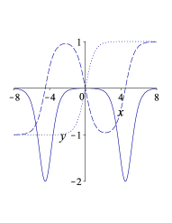
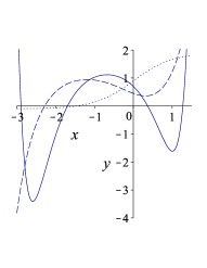
Figure 1: The double-well potential $V$ (solid line), the function $\chi$ (dashed line) and the multiplier-function $\phi$ (dotted line). For the symmetric case, (a, $\phi=\sinh(ax)/\cosh(bx)$, for the asymmetric case, (b, $\phi=\alpha+\tanh(\beta x)$. The symmetric case with parameters $a=\sqrt{-E_{0}}$, $b=\sqrt{-E_{1}}$, $E_{0}=-1$ and $E_{1}=-0.999$, features odd $\chi$ and $\phi$ functions, whereas for the asymmetric case (here with $\alpha=0.9$, $\beta=1$, $E_{0}=0$ and $E_{1}=1$) these symmetries are lost.

II.2 Symmetric Double-Well Potential

For the case of a symmetric double-well potential, as displayed in Figs. 1 a and 2, we use the multiplier-function

$$\phi(x)=\frac{\sinh(ax)}{\cosh(bx)}\;,$$ (8)

where (with $E_{0}<E_{1}<0$)

$$a=\sqrt{-E_{0}}\quad\mbox{ and }\quad b=\sqrt{-E_{1}}\;.$$ (9)

The function $\chi$ then takes the form

$$\chi(x)=\frac{\sinh(ax)\left(2b^{2}-2a^{2}\cosh^{2}(bx)\right)}{b\sinh(ax)\sinh(2bx)-2a\cosh(ax)\cosh^{2}(bx)}\\ +\frac{ab\cosh(ax)\sinh(2bx)}{b\sinh(ax)\sinh(2bx)-2a\cosh(ax)\cosh^{2}(bx)}$$ (10)

and the corresponding symmetric potential $V$ is

$$V(x)=\frac{2\left(b^{2}-a^{2}\right)\left(a^{2}\cosh^{2}(bx)+b^{2}\sinh^{2}(ax)\right)}{(a\cosh(ax)\cosh(bx)-b\sinh(ax)\sinh(bx))^{2}}\;.$$ (11)

The ground state $\psi_{0}$ (note typographical error in corresponding Eq. (19) of ref. Caticha (1995)), is

$$\psi_{0}(x)=\frac{\psi_{0}(0)(e^{2bx}+1)(a-b)e^{ax}}{(e^{2(b+a)x}+1)(a-b)+(a+b)(e^{2ax}+e^{2bx})}$$ (12)

and the first excited state $\psi_{1}$ is

$$\psi_{1}(x)=\frac{\psi_{1}(0)(e^{2ax}-1)(a-b)e^{bx}}{(e^{2(b+a)x}+1)(a-b)+(a+b)(e^{2ax}+e^{2bx})}\;.$$ (13)

The two wave functions have odd and even parity, see Fig. 2.

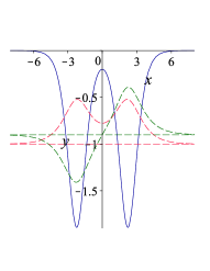
Figure 2: (Color Online) The symmetric double-well potential $V$ (solid blue line), the corresponding ground state $\psi_{0}$ (dashed red line) and the first excited state $\psi_{1}$ (dashed green line), for $E_{0}=-1$ and $E_{1}=-0.9$.

II.3 Asymmetric Double-Well Potential

With the multiplier-function $\phi$

$$\phi(x)=\alpha+\tanh(\beta x)$$ (14)

the function $\chi$ takes the form

$$\chi(x)=\frac{\Delta E}{4\beta}\left[\sinh(2\beta x)+2\alpha\cosh^{2}(\beta x)\right]-\beta\tanh(\beta x)$$ (15)

and the corresponding asymmetric potential $V$ is

$$V(x)=\beta^{2}-\Delta E\alpha\sinh(2\beta x)\\ +\cosh^{2}(\beta x)\left(\frac{\Delta E^{2}}{4\beta^{2}}\alpha\sinh(2\beta x)-\frac{\Delta E^{2}}{4\beta^{2}}-2\Delta E\right)\\ +\frac{\Delta E^{2}}{4\beta^{2}}\left(\alpha^{2}+1\right)\cosh^{4}(\beta x)+\frac{3}{2}\Delta E+E_{0}\;.$$ (16)

The corresponding lowest two wave functions are

$$\psi_{0}(x)=\psi_{0}(0)\cosh(\beta x)\\ \times\exp\left[-\frac{\Delta E}{4\beta^{2}}\left(\cosh^{2}(\beta x)+\alpha\beta x+\frac{\alpha}{2}\sinh(2\beta x)\right)\right]$$ (17)

and

$$\psi_{1}(x)=\psi_{1}(0)(\alpha\cosh(\beta x)+\sinh(\beta x))\\ \times\exp\left[-\frac{\Delta E}{4\beta^{2}}\left(\cosh^{2}(\beta x)+\alpha\beta x+\frac{\alpha}{2}\sinh(2\beta x)\right)\right]\;.$$ (18)

Fig. 3 illustrates that the potential’s asymmetry strongly modifies the shape of the lowest two wave functions as compared to the symmetric case, with $\alpha=0$, in Fig. 2.

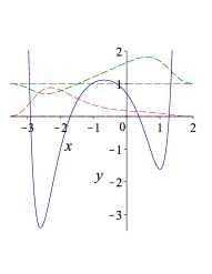
Figure 3: (Color Online) The asymmetric double-well potential $V$ (solid blue line), the corresponding ground state $\psi_{0}$ (dashed red line) and the first excited state $\psi_{1}$ (dashed green line), for $\alpha=0.9$, $\beta=1$, $E_{0}=0$ and $\Delta E=1$.

To investigate the tunneling dynamics we use the normalized superposition state

$$\Psi(x,t)=\sin(\theta)\exp\left(\frac{-iE_{0}t}{\hbar}\right)\psi_{0}(x)\\ +\cos(\theta)\exp\left(\frac{-iE_{1}t}{\hbar}\right)\psi_{1}(x)\;,$$ (19)

with the weighting angle $\theta\in[0,\ldots,\pi/2]$. The energy splitting $\Delta E$, gives rise to the beat period (or reciprocal barrier-tunneling rate Merzbacher (2002); Razavy (2003)) $T=2\pi\hbar/\Delta E$. In other words, $T$ is the time needed for a quantum particle initially localized in, say, the left well, to perform a full oscillation: left-right-left. The larger the energy splitting the shorter the beat period.

III Wigner’s Function

Eugene Wigner introduced his quasi-probability distribution function $W(x,p;t)$ in 1932 for the study of quantum corrections to classical statistical mechanics Wigner (1932). It is a generating function for all spatial auto-correlation functions of a given quantum mechanical wave function $\psi$ and defined as Razavy (2003); Wigner (1932); Belloni et al. (2004)

$$W(x,p;t)=\frac{1}{\pi\hbar}\int_{-\infty}^{\infty}{\Psi^{*}(x+y,t)\Psi(x-y,t)e^{\frac{2ipy}{\hbar}}dy}\;,$$ (20)

where $x$ and $y$ are position variables and $p$ the momentum. The Wigner quasi-probability distribution function is a real-valued phase-space distribution function, it can assume negative values which is why it is referred to as a quasi-probability distribution.

Its marginals are the quantum-mechanical probability distributions of position

$$P(x,t)=\left|\Psi(x,t)\right|^{2}=\int_{-\infty}^{\infty}{W(x,p;t)\;dp}$$ (21)

and momentum

$$\tilde{P}(p,t)=\left|\Phi(p,t)\right|^{2}=\int_{-\infty}^{\infty}{W(x,p;t)\;dx}\;.$$ (22)

It is normalized $\int_{-\infty}^{\infty}{\int_{-\infty}^{\infty}{W(x,p;t)\;dp}\;dx}=1\;$ and the overlap of the Wigner functions $W_{\psi}(x,p;t)$ and $W_{\chi}(x,p;t)$ of two distinct quantum states, $\psi(x,t)$ and $\chi(x,t)$, yields the magnitude of their wave function overlap squared Belloni et al. (2004)

$$\int_{-\infty}^{\infty}{\int_{-\infty}^{\infty}{W_{\psi}(x,p;t)W_{\chi}(x,p;t)\;dp}\;dx}=\frac{2}{\pi\hbar}\left|\left\langle\psi|\chi\right\rangle\right|^{2}.$$ (23)

Fig. 4 shows plots of the time evolution of the Wigner functions for symmetric and asymmetric double-well potentials and the associated marginals $P(x,t)$ and $\tilde{P}(p,t)$; all Wigner functions and marginals $\tilde{P}(p,t)$ had to be determined through numerical integrations.

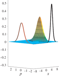
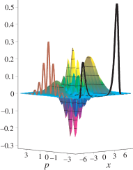
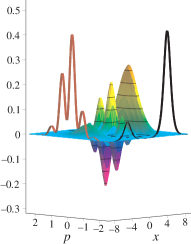
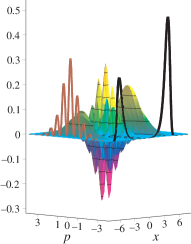
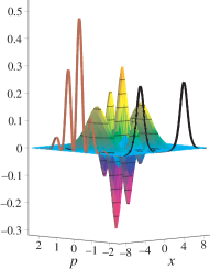
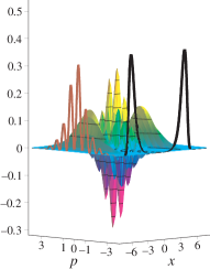
Figure 4: (Color Online) Time evolution of the Wigner quasi-probability distribution, for the symmetric double-well potential $V$ of Eq. (11) for $E_{0}=-1$ and $E_{1}=-0.999$, shown in subfigures a, b and c, and for the asymmetric double-well potential $V$ of Eq. (16) for $\alpha=0.9$, $\beta=1$, $E_{0}=0$ and $E_{1}=0.001$, shown in subfigures d, e and f, with weighting angle $\theta=\pi/4$. The projections of the Wigner function are the probability distributions with respect to position $P(x,t)$ (black) and momentum $\tilde{P}(p,t)/3$ (brown - shrunk by “$1/3$” for clarity and visibility).

III.1 Negative values of Wigner function

As can be seen from the projections of the Wigner quasi-probability distributions in Fig. 4, a particle that exists in two places at the same time shows interference fringes in its momentum probability distribution $\tilde{P}(p,t)$. These are incompatible with a single humped position distribution $P(x,t)$ in conjunction with a positive semi-definite phase space probability distribution. A phase space distribution simultaneously yielding such marginals has to contain regions with negative values. These negative regions are indicators of the non-classical character of the spatial coherences of the wave functions P. Schleich (2001) and are frequently studied in experiments Grangier (2011). They arise, e.g., whenever the wave function spreads out over both wells of the double-well potential.

To avoid confusion, we would like to emphasize that negative regions of the Wigner function, as a generating function for spatial auto-correlation functions, represent non-classical behavior of spatial correlations but not of the non-classical behavior of tunneling associated with “negative kinetic energy”. The interference fringes of the Wigner function, appearing roughly in the area where tunneling occurs, represent the non-classical spatial coherence of the wave functions located in both wells simultaneously.

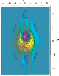
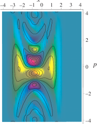
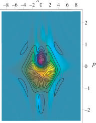
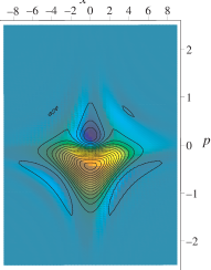
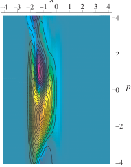
Figure 5: (Color Online - Color scheme identical to Fig. 4’s) The Wigner quasi-probability distribution for a range of values of the energy splitting $\Delta E$, for the symmetric double-well potential $V$ of Eq. (11) for $E_{0}=-1$ and $\Delta E=0.25,0.5\mbox{ and }0.75$, shown in subfigures a, b and c, respectively, and for the asymmetric double-well potential $V$ of Eq. (16) for $\alpha=0.9$, $\beta=1$, $E_{0}=0$ and for $\Delta E=0.5,4\mbox{ and }8$, shown in subfigures d, e and f, respectively, with weighting angle $\theta=\pi/4$ and $t=T/4$.

Fig. 5 illustrates the changes Wigner’s functions undergo when changing the potential wells from separate wells to merged single troughs (displayed in Fig. 6): Since the coupling between the wells increases, so does $\Delta E$. Concurrently the peaks of the spatial wave functions move together which increases the fringe spacing in the associated momentum representation, visible as a reduction of the spatial frequency of Wigner’s functions’ interference patterns.

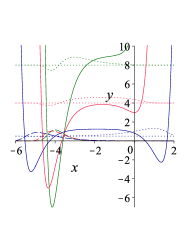
Figure 6: (Color Online) The symmetric double-well potential $V$ of Eq. (11), a, for $E_{0}=-1$ and $\Delta E=0.25,0.5\mbox{ and }0.75$, color blue, red and green, respectively, and the asymmetric double-well potential $V$ of Eq. (16), b, for $\alpha=0.9$, $\beta=1$, $E_{0}=0$ and $\Delta E=0.5,4\mbox{ and }8$, color blue, red and green, respectively, and their corresponding ground and first excited states, $\psi_{0}$ and $\psi_{1}$.

IV Conclusion

We have considered the effects of tunneling in smooth partially exactly solvable double-well potentials Caticha (1995). We illustrated the behavior of the associated wave functions and Wigner’s quasi-probability phase-space distributions. Wigner’s functions can assume negative values representing non-classical spatial coherences of the wave functions, these were shown to arise in the case of tunneling and analyzed and interpreted.

References

- Nimtz and Haibel (2008) G. Nimtz and A. Haibel, Zero Time Space (Wiley-VCH, KGaA, Weinheim, 2008).
- Merzbacher (2002) E. Merzbacher, Phys. Today 55, 080000 (2002).
- Razavy (2003) M. Razavy, Quantum Theory of Tunneling (World Scientific, Toh Tuck Link, Singapore, 2003).
- Ka and Shin (2003) J. Ka and S. Shin, J. Mol. Struct. 623, 23 (2003).
- Bai (2000) C. Bai, Scanning tunneling microscopy and its applications (Springer Verlag, New York, 2000).
- Carminati and Greffet (1995) R. Carminati and J. J. Greffet, Opt. Comm. 116, 316 (1995).
- Caticha (1995) A. Caticha, Phys. Rev. A 51, 4264 (1995).
- Gendenshteïn (1983) L. É. Gendenshteïn, J. Exp. Theor. Phys. Lett. 38, 356 (1983).
- Cooper et al. (1995) F. Cooper, A. Khare, and U. Sukhatme, Phys. Rep. 251, 267 (1995), arXiv:hep-th/9405029 .
- Wigner (1932) E. Wigner, Phys. Rev. 40, 749 (1932).
- Belloni et al. (2004) M. Belloni, M. A. Doncheski, and R. W. Robinett, Am. J. Phys. 72, 1183 (2004), arXiv:quant-ph/0312086 .
- P. Schleich (2001) W. P. Schleich, Quantum Optics in Phase Space (WILEY-VCH Verlag GmbH, Berlin, Germany, 2001).
- Grangier (2011) P. Grangier, Science 332, 313 (2011).